A Robust Optimization Model for
Nonlinear Support Vector Machine

Abstract

In this paper we present new optimization models for Support Vector Machine (SVM), with the aim of separating data points in two classes by means of a nonlinear classifier. Traditionally, in the nonlinear context data points are firstly mapped to a higher-dimensional space and then classified through a SVM-type model. In order to increase the predictive power of SVM, within our approach we include a final linear search procedure aiming to minimize the overall number of misclassified points. Along with a deterministic model in which data are assumed to be perfectly known, we formulate a robust optimization model with bounded-by-$\ell_{p}$-norm uncertainty sets. Indeed, when data are real-world observations, measurement errors or noise may corrupt the quality of input values. For this reason, facing uncertainty in the model is a way to robustify the approach. All formulations reduce to linear models with advantages in terms of efficiency compared to other approaches in the literature. Extensive numerical results on real-world datasets show the benefits in terms of accuracy when considering nonlinear decision classifier and protecting the model against uncertainties. Finally, managerial insights to guide the final user are provided.

1 Introduction

Support Vector Machine (SVM) is one of the main Machine Learning (ML) techniques commonly used for binary classification problems. Introduced in Vapnik (1982), within a few years it has outperformed most other ML systems, due to its simplicity and better performances (Peng and Xu (2013)). For these reasons, it has been applied in many practical research fields, such as finance (Luo et al. (2020), Tay and Cao (2001)), chemistry (Li et al. (2009)), renewable energy prediction (Zendehboudi et al. (2018)), medicine (Wang et al. (2018)), text classification (Tong and Koller (2002)), face recognition (Osuna et al. (1997)).
Classical SVM consists in finding a hyperplane classifying data into two classes, such that the margin, i.e. the distance from the hyperplane to the nearest point of each class, is maximized (Blanco et al. (2020)). Since data may not be perfectly linearly separable, the minimization of an empirical risk measure is included in the model (Cortes and Vapnik (1995)). In order to improve the accuracy of the method, several SVM variants have been proposed in the literature. Specifically, we focus our attention on the one presented in Liu and Potra (2009). According to this approach, data are firstly separated by means of two parallel hyperplanes and then the optimal hyperplane is searched in the strip between them, such that the total number of misclassified points is minimized.
Nevertheless, data points may not be always separable using linear classifiers, disrupting the reliability of the solution. In Boser et al. (1992), the extension of the linear SVM is introduced, by considering nonlinear transformation of the data. This approach considers the use of kernel function to embed data points in a higher-dimensional space, without increasing the computational complexity of the problem (Blanco et al. (2020)). Several variants of this technique have been proposed, by considering different properties of the problem (Mangasarian (1998), Schölkopf et al. (2000), Jayadeva et al. (2007), Peng (2011), Ding and Hua (2014), Blanco et al. (2020), Jiménez-Cordero et al. (2021)).
For the methods mentioned above, all data points are implicitly assumed to be known exactly. However, in real-world applications this condition may not be always true (Qi et al. (2013)). Indeed, measurement errors during data collection, random perturbations, presence of noise and other forms of uncertainty may corrupt the quality of input values, resulting in worsening performances of the algorithm. In recent years different techniques have been investigated with the aim of facing uncertainty in ML methods. Among them, Robust Optimization (RO) is one of the main paradigm to protect model against uncertainty (see Ben-Tal et al. (2009) and Xu et al. (2009)). RO assumes that all possible realizations of the uncertain parameter belong to a prescribed uncertainty set. The corresponding robust model is then obtained by optimizing against the worst-case realization of the parameter across the entire uncertainty set (Bertsimas et al. (2019)).
In this paper, we present a novel SVM-variant in the spirit of the approach of Liu and Potra (2009). The proposed model aims at generating two nonlinear decision boundaries such that all the points of a class lie on a specific side of the separators. The optimal classifier is finally searched in the region between them such that the misclassification error is minimized. Given the uncertain nature of real-world observations, we derive a robust counterpart of the deterministic model, by considering different kernel functions and uncertainty sets. The main contributions of the paper can be summarized as follows:

• To extend the linear SVM approach of Liu and Potra (2009) to the nonlinear context, by considering different kernel functions;

• To derive bounds on the uncertainty sets when considering nonlinear classifiers;

• To formulate a RO model of the approach of Liu and Potra (2009) with nonlinear classifiers;

• To provide extensive numerical experiments based on real-world datasets with the aim of evaluating the performances of the proposed models.

The remainder of the paper is organized as follows. Section 2 reviews the existing literature on the problem. In Section 3, the notation is introduced, along with a brief discussion on selected SVM-type problems. In Section 4, the novel deterministic model with nonlinear classifier is introduced. Section 5 considers the construction of uncertainty sets and presents the robust model. In Section 6, the computational results are shown. Finally, Section 7 concludes the paper and presents future developments of the work.

2 Literature review

SVM is introduced as a pattern recognition technique in Vapnik (1982) for the case of optimal hyperplane and with separable classes. The generalization of the linear approach is proposed in Boser et al. (1992), where input vectors are first compared by means of a distance measure and then mapped to a higher-dimensional space (the so-called feature space) via a nonlinear transformation. The main drawback of this approach is that training data points are considered separable. In Vapnik (1995) the shortcoming is overcome by relaxing the condition of perfect separability. Indeed, a soft margin error vector is introduced, and the corresponding optimal separation surface maximizes the margin for the correctly classified vectors and minimizes the magnitude of the soft margin error.
The approach presented so far has been applied to other nonlinear SVM variants, leading to alternative formulations. In Mangasarian (1998) a separating surface induced by a kernel matrix is derived by considering either a quadratic or piecewise-linear objective function. The corresponding model turns to be convex and is applied in Lee et al. (2000) to extract relevant features of breast cancer patients. In Schölkopf et al. (2000) the formulation of $\nu$-Support Vector Classification ($\nu$-SVC) is proposed for both linear and nonlinear classifiers. This class of algorithm differs from the classical SVM paradigm of Vapnik (1995) since it involves a new parameter $\nu$ in the objective function, controlling the number of support vectors. In Jayadeva et al. (2007) the Twin Support Vector Machine (TWSVM) is designed. Contrary to standard SVM, TWSVM determines two nonparallel hyperplanes by solving two small-sized SVM-type problems. This results in a reduced learning cost when compared to the classical SVM. In the nonlinear context, the nonparallel hyperplanes are deduced in the feature space, resulting in two nonlinear classifier in the input space. In this stream of research, Peng (2011) combines the TWSVM with a flexible parametric margin model, deriving the Twin Parametric Margin Support Vector Machine (TPMSVM). More recently, in Blanco et al. (2020) the classical $\ell_{2}$-norm problem has been extended to the more general case of $\ell_{p}$-norm with $p>1$. Second order cone formulations for the resulting dual and primal problems are then derived. The problem of feature selection in nonlinear SVM is explored in Jiménez-Cordero et al. (2021). The authors propose a method based on a min-max optimization problem, embedding a trade-off between model complexity and classification accuracy.
Up to this point, all the cited papers consider only the deterministic case of SVM, whose underlying hypothesis is that training data points are perfectly known. Unfortunately, in many real-world applications data are plagued by uncertainty caused by corruption or measurement errors. However, the classification algorithm should perform appropriately even after such perturbations (Singla et al. (2020)). Robust Optimization (RO) is one of the main paradigm to tackle the problem of dealing with uncertain data. Depending on the degree of information about data, different uncertainty sets may be constructed. Within the field of RO applied to linear SVM, in Bhattacharyya (2004) hyperellipsoids around data points are considered, leading to a Second Order Cone Programming (SOCP) formulation. A tractable robust counterpart of the classical SVM approach of Cortes and Vapnik (1995) is derived in Bertsimas et al. (2019). In particular, the authors robustify the soft margin SVM model against feature uncertainty by considering bounded-by-norm additive perturbations in the training data. In El Ghaoui et al. (2003) the binary classification problem under feature uncertainty is formulated with uncertainty sets in the form of hyperrectangles and hyperellipsoids around input data. With the same choices of uncertainty sets, in Faccini et al. (2022) a RO model of the linear SVM variant presented in Liu and Potra (2009) is proposed. The reader is referred to Wang and Pardalos (2014) for a survey on linear SVM under uncertainty.
As far as it concerns RO techniques applied to nonlinear SVM, different approaches exist in literature. In Bhadra et al. (2010) and Ben-Tal et al. (2012) the kernel matrix $K$ is assumed to be affected by uncertainty, due to feature perturbations in the input data. A decomposition of $K$ as a combination of positive semidefinite kernel matrices with bounded-by-$\ell_{p}$-norm coefficients is proposed. The main limitation of this approach is that the functional form of $K$ and of semidefinite kernel matrices is typically unknown. Thus, it is not obvious how to characterize the elements in the uncertainty set of $K$, unless by using a sampling procedure. Similarly, uncertainties in matrices are considered in Lanckriet et al. (2002), where the mean and the covariance matrix of each class are only known within some specified set, in the form of ellipsoids. In Bi and Zhang (2005) and in Trafalis and Gilbert (2006) data points in the input space are subject to unknown but bounded-by-$\ell_{p}$-norm perturbations. Robustified models are derived for both linear and nonlinear classifiers. In the latter case, when data are mapped to the feature space, an additive and unknown perturbation is introduced. The robustification of the nonlinear SVM problem leads to a tractable SOCP formulation. A related work on bounded uncertainty sets is Xu et al. (2009). The authors introduce sublinear aggregated uncertainty sets that generalize the classical notion of uncertainty set. Within this class, they prove that robustness in the feature space implies robustness in the input space. Besides, they link regularization to robustness and show that the kernelized SVM is implicitly a robust classifier without regularization in the feature space. A discussion about the relation between RO and regularization is also present in Singla et al. (2020). In Trafalis and Alwazzi (2010) the stability of linear and quadratic programming SVMs with bounded noise in the input space is investigated by using linear and nonlinear discriminant analysis. Polyhedral uncertainty sets are considered in Fan et al. (2014), Ju and Tian (2012) and Fung et al. (2002), based on the nonlinear classifier of Mangasarian (1998).
RO techniques are applied to other SVM-type problems. In Peng and Xu (2013) a robust TWSVM classifier is proposed, by considering data uncertainty in the variance matrices of the two classes. In Qi et al. (2013) and in Sahleh et al. (2022) robust counterparts of TWSVM and TPMSVM are derived. For the nonlinear case, only Gaussian kernel and ellipsoidal uncertainty sets around data points are considered, resulting in SOCP formulation. A complete survey on recent developments on TWSVM models can be found in Tanveer et al. (2022).
All the approaches discussed so far are listed in Table 1. For a comprehensive review of RO in the field of SVM the reader is referred to Singla et al. (2020).
The technique we propose in this contribution differs form the literature in several aspects. First of all, we present a novel optimization model with nonlinear classifier, extending the approach of Liu and Potra (2009). Secondly, we consider general bounded-by-$\ell_{p}$-norm uncertainty sets, deriving closed-form expressions of the bounds in the feature space for most of the typical used kernel function in ML literature. Furthermore, we derive the robust counterpart of the deterministic approach, protecting the model against uncertainty.

	SVM			Uncertainty (✓/ ✗)		Type of Robust Methodology
	Linear classifier	Nonlinear classifier				Box RO	Ellipsoidal RO	Polyhedral RO	Bounded by norm RO	Matrix RO
Vapnik (1982)	✓			✗
Boser et al. (1992)		✓		✗
Vapnik (1995)	✓	✓		✗
Mangasarian (1998)		✓		✗
Lee et al. (2000)		✓		✗
Schölkopf et al. (2000)	✓	✓		✗
Fung et al. (2002)	✓	✓		✓				✓
Lanckriet et al. (2002)	✓	✓		✓			✓			✓
El Ghaoui et al. (2003)	✓			✓		✓	✓
Bhattacharyya (2004)	✓			✓			✓
Bi and Zhang (2005)	✓	✓		✓					✓
Trafalis and Gilbert (2006)	✓	✓		✓					✓
Jayadeva et al. (2007)	✓	✓		✗
Liu and Potra (2009)	✓			✗
Xu et al. (2009)	✓	✓		✓					✓
Bhadra et al. (2010)		✓		✓						✓
Trafalis and Alwazzi (2010)	✓	✓		✓					✓
Peng (2011)	✓	✓		✗
Ben-Tal et al. (2012)		✓		✓					✓	✓
Ju and Tian (2012)	✓	✓		✓				✓
Peng and Xu (2013)	✓	✓		✓						✓
Qi et al. (2013)	✓	✓		✓			✓
Fan et al. (2014)	✓	✓		✓				✓
Bertsimas et al. (2019)	✓			✓					✓
Blanco et al. (2020)	✓	✓		✗
Jiménez-Cordero et al. (2021)		✓		✗
Faccini et al. (2022)	✓			✓		✓	✓
Sahleh et al. (2022)	✓	✓		✓			✓

Table 1: SVM literature review.

3 Background and notation

In this section, we report the notation and briefly recall some deterministic SVM-type model for pattern classification: the linear Soft Margin SVM (Vapnik (1995)), the Generalized SVM (Mangasarian (1998)) for nonlinear classification, and the Formulation II of Liu and Potra (2009) via misclassification minimization.

3.1 Notation

In the following, the set of nonnegative real numbers will be denoted by $\mathbb{R}^{+}$, whereas if zero is excluded we write $\mathbb{R}^{+}_{0}$. Hereinafter, all vectors will be column vectors, unless transposition by the superscript “^⊤”. If $a$ is a vector in $\mathbb{R}^{n}$, then its $i$-th component will be denoted by $a_{i}$ and $a=[a_{1},\ldots,a_{n}]^{\top}$. The scalar product in a inner product space $\mathcal{H}$ will be denoted by $\langle\cdot,\cdot\rangle$. If $\mathcal{H}=\mathbb{R}^{n}$ and $a,b\in\mathbb{R}^{n}$, the dot product will be indifferently denoted as $a^{\top}b$ or $\langle a,b\rangle$. For $p\in[1,\infty]$, $\left\lVert a\right\rVert_{p}$ is the $\ell_{p}$-norm of $a$. If $A$ is a matrix, $A_{i}$ denotes its $i$-th row. A column vector of ones of arbitrary dimension will be denoted by $e$. If $a,b\in\mathbb{R}^{n}$, the inequality $a\geq b$ shall be understood componentwise. Finally, if $c\in\mathbb{R}$, the indicator function $\mathbbm{1}(c)$ has value 1 if $c$ is positive and 0 otherwise.

3.2 A selected brief review of SVM deterministic models

Let $\{x^{(i)},y^{(i)}\}_{i=1}^{m}$ be the set of training data points, where $x^{(i)}\in\mathbb{R}^{n}$ is the vector of features, and $y^{(i)}\in\{-1,+1\}$ is the label representing the class to which the $i$-th data point belongs. In particular, we denote by $\mathcal{A}$ and $\mathcal{B}$ the class of positive (label “$+1$”) and negative (label “$-1$”) data points, respectively.

3.2.1 The Soft Margin Support Vector Machine

The Soft Margin SVM approach (SM-SVM), firstly introduced in Cortes and Vapnik (1995), finds the best separating hyperplane $H=(w,\gamma)$ defined by the equation $w^{\top}x=\gamma$, where $w\in\mathbb{R}^{n}$ and $\gamma\in\mathbb{R}$, as solution of the following $\ell_{q}$-model, $q>1$ (see Blanco et al. (2020)):

$$\min_{w,\gamma,\xi} \left\lVert w\right\rVert_{q}^{q}+\nu\sum_{i=1}^{m}\xi_{i}$$ (1)

s.t. $$y^{(i)}(w^{\top}x^{(i)}-\gamma)\geq 1-\xi_{i} \quad i=1,\ldots,m$$

$$\xi_{i}\geq 0 \quad i=1,\ldots,m.$$

The vector $\xi\in\mathbb{R}^{m}$ is the soft margin error vector and $\nu\geq 0$ is a regularization parameter, balancing the trade-off between the maximization of the margin (i.e. the minimization of $\left\lVert w\right\rVert_{q}^{q}$), and the minimization of the misclassification error. Indeed, data point $x^{(i)}$ is correctly classified by the separating hyperplane, i.e. it lies on the correct side of $H$, if $0\leq\xi_{i}\leq 1$, otherwise is misclassified.
A new data point $x\in\mathbb{R}^{n}$ is classified as positive or negative depending on the decision function $\mathbbm{1}\big{(}w^{\top}x-\gamma\big{)}$: if it is equal to 1, then $x$ is assigned to class $\mathcal{A}$, otherwise to class $\mathcal{B}$.

3.2.2 The Formulation II of Liu and Potra (2009)

Instead of a single hyperplane as in the case of classical SM-SVM, in Liu and Potra (2009) a novel approach involving two parallel hyperplanes is proposed.
The starting point of the formulation employs the solutions of model (1) with $q=1$, specifically hyperplane $H_{0}=(w,\gamma)$ and the soft margin error vector $\xi$. Once $H_{0}$ and $\xi$ are obtained, the hyperplane $H_{0}$ is shifted in order to determine two parallel hyperplanes $H_{\mathcal{A}}:=(w,\gamma-1+\omega_{A})$ and $H_{\mathcal{B}}:=(w,\gamma+1-\omega_{B})$, where:

$$\omega_{\mathcal{A}}:=\max_{i:x^{(i)}\in\mathcal{A}}\big{\{}\xi_{i}\big{\}},\quad\omega_{\mathcal{B}}:=\max_{i:x^{(i)}\in\mathcal{B}}\big{\{}\xi_{i}\big{\}},$$ (2)

satisfying the following properties:

1. all points of $\mathcal{A}$ lie on one side of $H_{\mathcal{A}}$;

2. all points of $\mathcal{B}$ lie on the opposite side of $H_{\mathcal{B}}$;

3. the intersection of the convex hulls of the two classes is contained in the strip between $H_{\mathcal{A}}$ and $H_{\mathcal{B}}$.

Finally, the optimal separating hyperplane $H=(w,b)$ is parallel to $H_{\mathcal{A}}$ and $H_{\mathcal{B}}$, lies in their strip, and is such that the number of misclassified points is minimized. These conditions are met by the optimal parameter $b$, solution of the following problem:

$$\min_{b} \sum_{i:x^{(i)}\in\mathcal{A}}\mathbbm{1}\big{(}w^{\top}x^{(i)}-b\big{)}+\sum_{i:x^{(i)}\in\mathcal{B}}\mathbbm{1}\big{(}b-w^{\top}x^{(i)}\big{)}$$ (3)

s.t. $$\gamma+1-\omega_{\mathcal{B}}\leq b\leq\gamma-1+\omega_{\mathcal{A}}.$$

Similarly to SM-SVM, a new data point $x\in\mathbb{R}^{n}$ is classified in class $\mathcal{A}$ or $\mathcal{B}$ depending on the decision rule $\mathbbm{1}\big{(}w^{\top}x-b\big{)}$.

3.2.3 The Generalized Support Vector Machine

Data points coming from real-world measurements may not be always separable by means of an hyperplane and, even with ad hoc variants of linear SVM, the misclassification error may be significant. This observation motivates the idea of considering nonlinear separating surfaces induced by a kernel function (see Cortes and Vapnik (1995)).
The idea behind this approach is the following: the training data points are mapped into a higher-dimensional space $\mathcal{H}$, where a separating hyperplane is constructed, yielding to a nonlinear decision surface in $\mathbb{R}^{n}$. Specifically, a function $\phi(\cdot)$, usually referred as feature map (see Schölkopf and Smola (2001)), is introduced to map data from the input space $\mathbb{R}^{n}$ to a feature space $\mathcal{H}$, equipped with the dot product $\langle\cdot,\cdot\rangle$.
Thus, model (1) in the feature space becomes:

$$\min_{\overline{w},\gamma,\xi} \left\lVert\overline{w}\right\rVert_{\mathcal{H}}+\nu\sum_{i=1}^{m}\xi_{i}$$ (4)

s.t. $$y^{(i)}(\langle\overline{w},\phi(x^{(i)})\rangle-\gamma)\geq 1-\xi_{i} \quad i=1,\ldots,m$$

$$\xi_{i}\geq 0 \quad i=1,\ldots,m,$$

where $\overline{w}$ refers to the vector defining the linear classifier in the feature space and the norm in $\mathcal{H}$ is induced by its inner product, i.e., for $z\in\mathcal{H}$, $\left\lVert z\right\rVert_{\mathcal{H}}:=\sqrt{\langle z,z\rangle}$.
As in Cortes and Vapnik (1995), the vector $\overline{w}$ can be decomposed as a finite linear combination of $\phi(x^{(j)})$, $j=1,\ldots,m$:

$$\overline{w}=\sum_{j=1}^{m}y^{(j)}u_{j}\phi(x^{(j)}),$$ (5)

for some coefficients $u_{j}\in\mathbb{R}$. Unfortunately, the expression of the mapping $\phi(\cdot)$ is usually unknown and, consequently, model (4) cannot be solved in practice (see Jiménez-Cordero et al. (2021)). To overcome this problem, a symmetric and positive definite kernel $k:\mathbb{R}^{n}\times\mathbb{R}^{n}\to\mathbb{R}$ is introduced to measure the similarity of two observations (see Schölkopf and Smola (2001)). Examples of kernel function typically used in ML literature are reported in Table 2. For a comprehensive overview, the reader is referred to Schölkopf and Smola (2001).

Kernel function	$k(x,x^{\prime})$	Parameter
Homogeneous polynomial	$k(x,x^{\prime})=\langle x,x^{\prime}\rangle^{d}$	$d\in\mathbb{N}$
Inhomogeneous polynomial	$k(x,x^{\prime})=(c+\langle x,x^{\prime}\rangle)^{d}$	$c\in\mathbb{R}^{+}$, $d\in\mathbb{N}$
Gaussian RBF	$k(x,x^{\prime})=\exp\bigg{(}\displaystyle-\frac{\left\lVert x-x^{\prime}\right\rVert_{2}^{2}}{2\alpha^{2}}\bigg{)}$	$\alpha\in\mathbb{R}^{+}_{0}$
Sigmoid	$k(x,x^{\prime})=\tanh(a\text{ }\langle x,x^{\prime}\rangle+b)$	$a\in\mathbb{R}$, $b\in\mathbb{R}$

Table 2: Examples of kernel functions. RBF stands for “Radial Basis Function”.

Let $K$ be the Gram matrix associated to the kernel $k(\cdot,\cdot)$, i.e., $K_{ij}:=k(x^{(i)},x^{(j)})=\langle\phi(x^{(i)}),\phi(x^{(j)})\rangle$. The properties of $k(\cdot,\cdot)$ imply that $K$ is a real, symmetric and positive definite $m\times m$ matrix (see Schölkopf and Smola (2001)).
Consequently, for all $i=1,\ldots,m$ the scalar product $\langle\overline{w},\phi(x^{(i)})\rangle$ in the first set of constraints of model (4) can be formulated as:

$$\langle\overline{w},\phi(x^{(i)})\rangle=\sum_{j=1}^{m}y^{(j)}u_{j}\langle\phi(x^{(j)}),\phi(x^{(i)})\rangle=\sum_{j=1}^{m}K_{ij}y^{(j)}u_{j}=K_{i}Du,$$

where $D$ is a diagonal matrix with $D_{ii}:=y^{(i)}$ and $u=[u_{1},\ldots,u_{m}]^{\top}$. Furthermore, the norm $\left\lVert\overline{w}\right\rVert_{\mathcal{H}}$ can be expressed in terms of matrices $K$ and $D$ as:

$$\left\lVert\overline{w}\right\rVert_{\mathcal{H}}^{2}=\langle\overline{w},\overline{w}\rangle=\sum_{i=1}^{m}\sum_{j=1}^{m}y^{(i)}y^{(j)}u_{i}u_{j}k(x^{(i)},x^{(j)})=(Du)^{\top}K(Du).$$

Due to the structure of $D$, containing only $1$ and $-1$ elements in the diagonal, it holds that $\left\lVert Du\right\rVert_{q}=\left\lVert u\right\rVert_{q}$, for all $q\in[1,\infty]$. Besides, equality (5) states that vector $\overline{w}$ depends linearly on its coefficients $u_{j}$. Thus, as suggested in Lee et al. (2000), in order to minimize $\left\lVert\overline{w}\right\rVert_{\mathcal{H}}$ we minimize the magnitude of $\left\lVert u\right\rVert_{q}$. Therefore, model (4) can be written as:

$$\min_{u,\gamma,\xi} \left\lVert u\right\rVert_{q}^{q}+\nu\sum_{i=1}^{m}\xi_{i}$$ (6)

s.t. $$y^{(i)}\bigg{(}\sum_{j=1}^{m}K_{ij}y^{(j)}u_{j}-\gamma\bigg{)}\geq 1-\xi_{i} \quad i=1,\ldots,m$$

$$\xi_{i}\geq 0 \quad i=1,\ldots,m,$$

or, equivalently, in matrix form:

$$\min_{u,\gamma,\xi} \left\lVert u\right\rVert_{q}^{q}+\nu e^{\top}\xi$$ (7)

s.t. $$D(KDu-e\gamma)\geq e-\xi$$

$$\xi\geq 0.$$

Model (7) with $q=1$ corresponds to the Generalized Support Vector Machine (G-SVM) presented in Mangasarian (1998).
Within this context, the hyperplane in the feature space translates into a nonlinear separating surface $S$ in the input space, induced by the kernel function $k(\cdot,\cdot)$. Surface $S$ is defined implicitly by the following equation:

$$\sum_{i=1}^{m}k(x,x^{(i)})y^{(i)}u_{i}=\gamma,$$ (8)

where $u\in\mathbb{R}^{m}$ and $\gamma\in\mathbb{R}$ are the solutions of program (6). Hereinafter, coherently with the linear case, a surface $S$ in the input space satisfying equation (8) will be denoted by $S:=(u,\gamma)$.
When a new data point $x\in\mathbb{R}^{n}$ occurs, it is classified either in class $\mathcal{A}$ or $\mathcal{B}$ according to whether the decision function

$$\mathbbm{1}\bigg{(}\sum_{i=1}^{m}k(x,x^{(i)})y^{(i)}u_{i}-\gamma\bigg{)}$$

yields 1 or 0, respectively.

4 A novel approach for deterministic nonlinear SVM

After having reviewed selected variants of linear and nonlinear SVM, we devote this section to extending the linear approach of Liu and Potra (2009) to the nonlinear case. Thus, we derive nonlinear separating surfaces in the input space, satisfying the aforementioned properties (P1)-(P3).
First of all, by solving model (6), we find an initial surface $S_{0}:=(u,\gamma)$ which induces a first nonlinear separation in the input space. The nonlinear surface $S_{0}$ corresponds to a linear classifier $H_{0}$ in the feature space. As in Liu and Potra (2009), we set $q=1$, corresponding to the maximization of the margin with respect to the $\ell_{\infty}$-norm. This choice provides a good compromise between structural risk minimization, related to the misclassification error, and parsimony since it automatically performs feature selection, by making zero nonrelevant components of the normal vector $u$ (see López et al. (2019)). Moreover, with $q=1$, problem (6) reduces to a linear problem.
Then, as in (2), for each of the two classes, we compute the greatest misclassification error. This can be performed efficiently through the following formulas:

$$\omega_{\mathcal{A}}:=\max_{i=1,\ldots,m}{(D\xi)}_{i}\qquad\omega_{\mathcal{B}}:=\max_{i=1,\ldots,m}{(-D\xi)}_{i}.$$ (9)

Due to the structure of problem (6), the modulus of $-1+\omega_{\mathcal{A}}$ represents the distance of the farthest misclassified point of class $\mathcal{A}$ from $H_{0}$ in the feature space, and similarly for $1-\omega_{\mathcal{B}}$. However, it may happen that $H_{0}$ already classifies correctly all the data points of at least one of the two classes. Assume, without loss of generality, that it happens for class $\mathcal{A}$. This implies that $0\leq\xi_{i}\leq 1$, for all $i$ such that $x^{(i)}\in\mathcal{A}$. Thus, the modulus of $-1+\omega_{\mathcal{A}}$ is just the distance from the closest data points in $\mathcal{A}$ to the hyperplane $H_{0}$. Accordingly to the literature of SVM (see Cortes and Vapnik (1995)), we call the points at distance $\left\lvert-1+\omega_{\mathcal{A}}\right\rvert$ and $\left\lvert 1-\omega_{\mathcal{B}}\right\rvert$ the support vectors of class $\mathcal{A}$ and $\mathcal{B}$, respectively.
After the computation of $\omega_{\mathcal{A}}$ and $\omega_{\mathcal{B}}$, we shift $H_{0}$ by $-1+\omega_{\mathcal{A}}$ and $1-\omega_{\mathcal{B}}$ in the feature space, getting two parallel hyperplanes to $H_{0}$, namely $H_{\mathcal{A}}$ and $H_{\mathcal{B}}$, passing through the support vectors of the corresponding class. In the input space two nonlinear surface $S_{\mathcal{A}}$ and $S_{\mathcal{B}}$ are derived, defined as $S_{\mathcal{A}}:=(u,\gamma-1+\omega_{\mathcal{A}})$ and $S_{\mathcal{B}}:=(u,\gamma+1-\omega_{\mathcal{B}})$, respectively, accordingly to equation (8). With this choice, properties (P1)-(P2) are satisfied by $H_{\mathcal{A}}$ and $H_{\mathcal{B}}$ in the feature space, and by $S_{\mathcal{A}}$ and $S_{\mathcal{B}}$ in the input space.
Within this nonlinear approach, it is straightforward to notice that a strip between $S_{\mathcal{A}}$ and $S_{\mathcal{B}}$ does not exist in the input space, unless $k(\cdot,\cdot)$ is the linear kernel and the surfaces reduce to hyperplanes (see Table 2 in the case of homogeneous polynomial kernel with $d=1$). However, even in this situation, $S_{0}$, $S_{\mathcal{A}}$ and $S_{\mathcal{B}}$ do not intersect each other. Indeed, the definitions of $S_{0}$, $S_{\mathcal{A}}$ and $S_{\mathcal{B}}$ imply that the left-hand side of equation (8) is the same for all three, whereas only the constant term in the right-hand side changes.
Finally, the optimal separating surface $S:=(u,b)$ is obtained. The parameter $b$ is the solution of the following linear search procedure, similar to (3), aiming to minimize the overall number of misclassified points:

$$\min_{b} \sum_{i=1}^{m}\mathbbm{1}\bigg{(}y^{(i)}b-y^{(i)}\sum_{j=1}^{m}K_{ij}y^{(j)}u_{j}\bigg{)}$$ (10)

s.t. $$\gamma+1-\omega_{\mathcal{B}}\leq b\leq\gamma-1+\omega_{\mathcal{A}}.$$

The surface $S$ in the input space is induced by an hyperplane $H$ in the feature space, lying in the strip between $H_{\mathcal{A}}$ and $H_{\mathcal{B}}$, and satisfying property (P3).
In a similar way to G-SVM, a new observation $x\in\mathbb{R}^{n}$ is classified according to the decision function:

$$\mathbbm{1}\bigg{(}\sum_{i=1}^{m}k(x,x^{(i)})y^{(i)}u_{i}-b\bigg{)}.$$

For the sake of clarity, all the steps of the approach discussed so far are schematically reported in Pseudocode 1.

0:  $\{x^{(i)},y^{(i)}\}_{i=1}^{m}$, $\nu\geq 0$, $k(\cdot,\cdot):\mathbb{R}^{n}\times\mathbb{R}^{n}\to\mathbb{R}$.

1:  Calculate matrix $K_{ij}=k\big{(}x^{(i)},x^{(j)}\big{)},i,j=1,\ldots,m$ and the diagonal matrix of the labels $D_{ii}=y^{(i)},i=1,\ldots,m$.

2:  Solve model (6) with $q=1$.

3:  Find the initial separating surface $S_{0}=(u,\gamma)$, defined by equation (8).

4:  Compute $\omega_{\mathcal{A}}$ and $\omega_{\mathcal{B}}$, according to formulas (9).

5:  Shift $S_{0}$ to get the separating surface for each class, $S_{\mathcal{A}}=(u,\gamma-1+\omega_{\mathcal{A}})$ and $S_{\mathcal{B}}=(u,\gamma+1-\omega_{\mathcal{B}})$, defined by (8).

6:  Solve model (10), obtaining the optimal parameter $b$.

6:  The optimal decision boundary $S=(u,b)$, defined by (8).

Pseudocode 1 A novel approach for deterministic nonlinear SVM

4.1 An illustrative example

We sketch in Figure 1 the results of the approach presented in the previous section when applied to a bidimensional toy example.

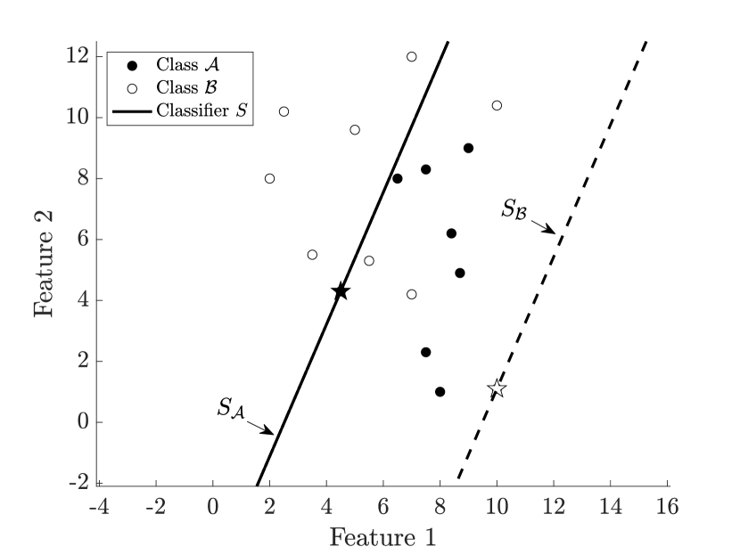
(a) Linear kernel

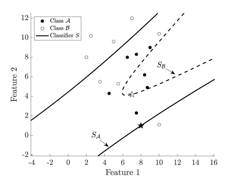
(b) Quadratic kernel

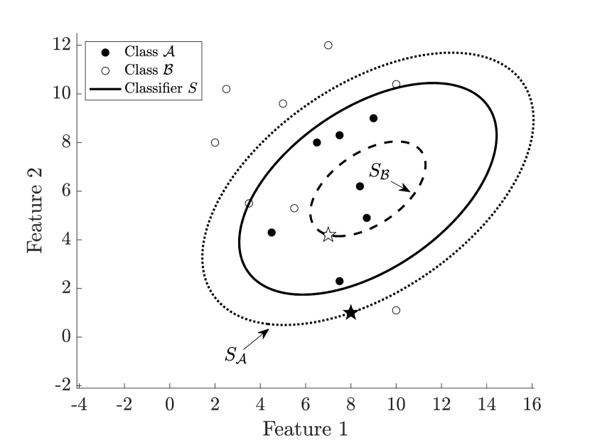
(c) Inhomogeneous quadratic kernel ($c=0.3$)

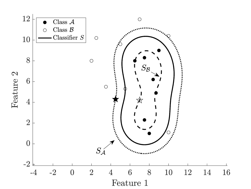
(d) Gaussian RBF kernel ($\alpha=1.9$)

Figure 1: Separating surfaces obtained with different kernel functions. Support vectors are depicted as stars.

The parameter $\nu$ in the objective function of (6) has been set to 1, and the classification performed by choosing four different kernel functions: linear kernel (namely, homogeneous polynomial kernel with degree $d=1$); quadratic polynomial kernel (homogeneous polynomial kernel with $d=2$); inhomogeneous quadratic polynomial kernel with $c=0.3$; Gaussian RBF kernel with $\alpha=1.9$.
The optimal separating surface $S$ is represented by a solid line, whereas surfaces $S_{\mathcal{A}}$ and $S_{\mathcal{B}}$ are depicted as dotted and dashed line, respectively. The support vectors are drawn as stars. Depending on the choice of the kernel function, it may happen that $S$ coincides either with $S_{\mathcal{A}}$ or $S_{\mathcal{B}}$ (see for instance Figures 1(a)-1(b)). In any case, as expected, both $S_{\mathcal{A}}$ and $S_{\mathcal{B}}$ satisfy properties (P1)-(P2). Indeed, by considering for example Figure 1(c), all the black points of class $\mathcal{A}$ lie inside the ellipse defined by $S_{\mathcal{A}}$, and all the white points of class $\mathcal{B}$ are outside $S_{\mathcal{B}}$. Moreover, the optimal surface $S$ satisfies property (P3) since it is comprised in the region between $S_{\mathcal{A}}$ and $S_{\mathcal{B}}$, and minimizes the total number of misclassified points.
In general, it is difficult to know in advance which kernel function is more suitable for a particular dataset (de Diego et al. (2009)). Even in the considered bidimensional toy example, the performance strongly varies on the basis of the kernel. Indeed, the total number of misclassified points is 4 for the linear and quadratic kernels, 3 for the inhomogeneous quadratic kernel, and 2 for the Gaussian RBF kernel, which has the best performance within this example.

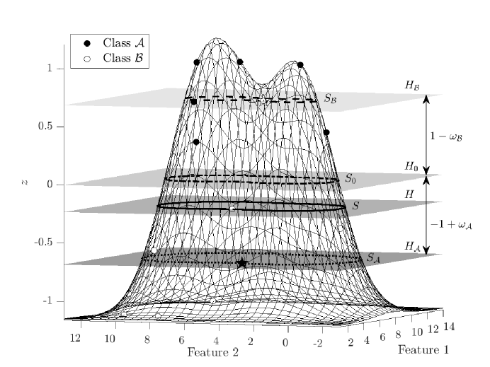
Figure 2: Graphical representation of the implicit function (8), in the case of Gaussian RBF kernel, along with the separating hyperplanes and surfaces. Support vectors are drawn as stars.

To conclude, we visualize in Figure 2 the 3D interpretation of the novel approach, applied to the same toy dataset of Figure 1, in the case of Gaussian RBF kernel with $\alpha=1.9$. Each data point is mapped through the implicit function defined by (8), with $u$ and $\gamma$ solutions of model (6), and the first separating hyperplane $H_{0}$ is correspondingly derived. Then, $H_{0}$ is parallelly shift by $-1+\omega_{\mathcal{A}}$ and $1-\omega_{\mathcal{B}}$, in order to get $H_{\mathcal{A}}$ and $H_{\mathcal{B}}$, and passing through the support vectors of the two classes. Once again, properties (P1)-(P2) are satisfied, since all the points of class $\mathcal{A}$ and $\mathcal{B}$ lie, respectively, above $H_{\mathcal{A}}$ and below $H_{\mathcal{B}}$. The optimal hyperplane $H$ is searched in the strip between $H_{\mathcal{A}}$ and $H_{\mathcal{B}}$. Finally, the four hyperplanes are projected onto the input space $\mathbb{R}^{2}$ and the optimal nonlinear separating surfaces are the corresponding contour lines, leading to Figure 1(d).

5 A robust model for nonlinear SVM

In this section, we derive the robust counterpart of the deterministic model introduced in the previous section, considering uncertainties in the input data. Within the robust approach, such uncertainties are taken into consideration when training the classifier by constructing an uncertainty set $\mathcal{U}(x^{(i)})$ around each observation $x^{(i)}$ (Bertsimas and Brown (2009)). Thus, the problem is to optimize against the worst-case realization across the entire uncertainty sets of all the observations (Bertsimas et al. (2019)). The uncertainty set can be defined in different ways, according to the degree of uncertainty that is considered in the model. Typically box, ellipsoidal and polyhedral uncertainty sets are considered because they lead to tractable optimization models (El Ghaoui et al. (2003), López et al. (2019), Fan et al. (2014)).
The robust counterpart of the Liu and Potra linear model is derived in Faccini et al. (2022), where the uncertainty sets are modelled as box or ellipsoids. Unfortunately, in the nonlinear context, when data points $x^{(i)}$ are mapped in the feature space $\mathcal{H}$ via $\phi(\cdot)$, a priori control about the shape and the properties of the uncertainty set $\mathcal{U}\big{(}\phi(x^{(i)})\big{)}$ is not available. In addition, a closed-form expression of $\phi(\cdot)$ is rarely available. Therefore, further assumptions when constructing $\mathcal{U}\big{(}\phi(x^{(i)}\big{)}$ have to be made.
The remainder of the section is organized as follows. In Subsection 5.1 uncertainty sets bounded by a general $\ell_{p}$-norm are constructed by considering different kernel functions. In Subsection 5.2 the robust counterpart of model (6) is derived.

5.1 The construction of the uncertainty set

As in Trafalis and Gilbert (2006), we assume that each observation $x^{(i)}$ in the input space is subject to an additive and unknown perturbation vector $\sigma^{(i)}$. In addition, we assume that its $\ell_{p}$-norm, with $p\in[1,\infty]$, can be bounded by a known nonnegative constant $\eta^{(i)}$. Therefore, the uncertainty set in the input space has the following expression:

$$\mathcal{U}_{p}(x^{(i)}):=\Set{x\in\mathbb{R}^{n}:x=x^{(i)}+\sigma^{(i)},\lVert\sigma^{(i)}\lVert_{p}\leq\eta^{(i)}},$$ (11)

with $p\in[1,\infty]$. The nonnegative parameter $\eta^{(i)}$ calibrates the degree of conservatism. If $\eta^{(i)}=0$, then $\sigma^{(i)}$ is the null vector and $\mathcal{U}_{p}(x^{(i)})$ coincides with $x^{(i)}$. Different $\ell_{p}$-norms lead to different geometrical properties of $\mathcal{U}_{p}(x^{(i)})$: $\ell_{1}$-norm, $\ell_{2}$-norm and $\ell_{\infty}$-norm yields to polyhedral, ellipsoidal and box uncertainty set, respectively.
Let us now assume that, if $x$ belongs to $\mathcal{U}_{p}(x^{(i)})$, then:

$$\phi(x)=\phi(x^{(i)}+\sigma^{(i)})=\phi(x^{(i)})+\zeta^{(i)},$$

where the perturbation $\zeta^{(i)}$ belongs to the feature space $\mathcal{H}$ and its $\mathcal{H}$-norm is bounded a nonnegative constant $\delta^{(i)}$. The latter may be unknown but, in turn, depends on the known bound $\eta^{(i)}$ in the input space, i.e. $\delta^{(i)}=\delta^{(i)}\big{(}\eta^{(i)}\big{)}$. If no uncertainty occurs in the input space, no uncertainty will occur in the feature space too. Thus, $\eta^{(i)}=0$ implies $\delta^{(i)}=0$. Hence, the uncertainty set in the feature space is modelled as:

$$\mathcal{U}_{\mathcal{H}}\big{(}\phi(x^{(i)})\big{)}:=\Set{z\in\mathcal{H}:z=\phi(x^{(i)})+\zeta^{(i)},\lVert\zeta^{(i)}\lVert_{\mathcal{H}}\leq\delta^{(i)}}.$$ (12)

In the case of homogeneous polynomial kernel, inhomogeneous polynomial kernel and Gaussian RBF kernel, it is possible to derive a closed-form expression for the bound $\delta^{(i)}$ in the feature space, knowing the bound $\eta^{(i)}$ in the input space. Before stating these results, we recall some useful norm inequalities in $\mathbb{R}^{n}$.

Lemma 1 (Inequalities in $\ell_{p}$-norm).

Let $x$ be a vector in $\mathbb{R}^{n}$. If $1\leq p\leq q\leq\infty$, then:

$$\left\lVert x\right\rVert_{q}\leq\left\lVert x\right\rVert_{p}\leq n^{\textstyle\frac{1}{p}-\frac{1}{q}}\left\lVert x\right\rVert_{q}.$$ (13)

By convention, we assume that $\frac{1}{\infty}=0$. The proof of the lemma is reported in A.
As special cases, Lemma 1 implies that, whenever $1\leq p\leq 2$, then:

$$\left\lVert x\right\rVert_{2}\leq\left\lVert x\right\rVert_{p}.$$ (14)

Conversely, if $p>2$, then:

$$\left\lVert x\right\rVert_{2}\leq n^{\textstyle\frac{p-2}{2p}}\left\lVert x\right\rVert_{p}.$$ (15)

Thus, combining these results, we can write in a compact way that:

$$\left\lVert x\right\rVert_{2}\leq C\left\lVert x\right\rVert_{p},$$

with:

$$C=C(n,p)=\begin{cases}1,&1\leq p\leq 2\\ n^{\textstyle\frac{p-2}{2p}},&p>2.\end{cases}$$ (16)

Let us now consider a symmetric and positive definite kernel $k(\cdot,\cdot)$, whose corresponding feature map is $\phi(\cdot)$. The $\mathcal{H}$-norm of the vector of perturbation $\zeta^{(i)}$ in the feature space can be expanded as:

$$\begin{split}\left\lVert\zeta^{(i)}\right\rVert^{2}_{\mathcal{H}}&=\left\lVert\phi(x)-\phi(x^{(i)})\right\rVert^{2}_{\mathcal{H}}\\ &=\left\lVert\phi(x^{(i)}+\sigma^{(i)})-\phi(x^{(i)})\right\rVert^{2}_{\mathcal{H}}\\ &=\langle\phi(x^{(i)}+\sigma^{(i)})-\phi(x^{(i)}),\phi(x^{(i)}+\sigma^{(i)})-\phi(x^{(i)})\rangle\\ &=\langle\phi(x^{(i)}+\sigma^{(i)}),\phi(x^{(i)}+\sigma^{(i)})\rangle-2\langle\phi(x^{(i)}+\sigma^{(i)}),\phi(x^{(i)}\rangle+\\ &\quad+\langle\phi(x^{(i)}),\phi(x^{(i)})\rangle\\ &=k(x^{(i)}+\sigma^{(i)},x^{(i)}+\sigma^{(i)})-2k(x^{(i)}+\sigma^{(i)},x^{(i)})+k(x^{(i)},x^{(i)}).\end{split}$$ (17)

In the following, we derive closed-form expressions for the bound $\delta^{(i)}$ by analysing separately the polynomial kernel and the Gaussian RBF kernel.

Lemma 2 (Polynomial kernel).

Let $\mathcal{U}_{p}(x^{(i)})$ and $\mathcal{U}_{\mathcal{H}}\big{(}\phi(x^{(i)})\big{)}$ be the uncertainty sets in the input and in the feature space as in (11) and (12), respectively, with $p\in[1,\infty]$. Consider the inhomogeneous polynomial kernel of degree $d\in\mathbb{N}$ and additive constant $c\geq 0$.

• If $d=1$, then the bound in the feature space is:

  $$\delta^{(i)}_{\text{lin}}=C\eta^{(i)}.$$ (18)

• If $d>1$, then:

  $$\delta^{(i)}_{\text{inhom}}=\sqrt{\big{(}\delta^{(i)}_{\text{hom}}\big{)}^{2}+\sum_{k=1}^{d-1}\binom{d}{k}c^{k}\bigg{[}\sum_{j=1}^{d-k}\binom{d-k}{j}\left\lVert x^{(i)}\right\rVert_{2}^{d-k-j}\big{(}C\eta^{(i)}\big{)}^{j}\bigg{]}^{2}},$$ (19)

  where $\delta^{(i)}_{\text{hom}}$ is the bound for the corresponding homogeneous polynomial kernel:

  $$\delta^{(i)}_{\text{hom}}=\sum_{k=1}^{d}\binom{d}{k}\left\lVert x^{(i)}\right\rVert_{2}^{d-k}\big{(}C\eta^{(i)}\big{)}^{k}.$$ (20)

The constant $C$ depends on the number of features $n$ and on the norm $p$.

When $c=0$, the bound $\delta^{(i)}_{\text{inhom}}$ in (19) reduces to $\delta^{(i)}_{\text{hom}}$ in (20).

Lemma 3 (Gaussian RBF kernel).

Let $\mathcal{U}_{p}(x^{(i)})$ and $\mathcal{U}_{\mathcal{H}}\big{(}\phi(x^{(i)})\big{)}$ be the uncertainty sets in the input and in the feature space as in (11) and (12), respectively, with $p\in[1,\infty]$. If $k(\cdot,\cdot)$ is the Gaussian RBF kernel with parameter $\alpha>0$, then:

$$\delta^{(i)}_{\text{RBF}}=\sqrt{2-2\exp\bigg{(}\displaystyle-\frac{{(C\eta^{(i)})}^{2}}{2\alpha^{2}}\bigg{)}},$$ (21)

with constant $C$ given in (16).

The proofs of Lemmas 2-3 are reported in A.
As mentioned above, when no corruption occurs in the data, $\eta^{(i)}=0$ and thus $\delta^{(i)}=0$. In addition, the two Lemmas 2-3 are consistent with Lemma 7 presented in Xu et al. (2009). However, in this contribution we specify the bound for particular kernels and extend the results for an uncertainty set bounded-by-$\ell_{p}$-norm, for a generic $p\in[1,\infty]$.

5.2 The robust model

Robustifying model (6) against the uncertainty set $\mathcal{U}_{p}(x^{(i)})$ yields the following robust optimization program: 0pt

$$\min_{u,\gamma,\xi} \left\lVert u\right\rVert_{1}+\nu\sum_{i=1}^{m}\xi_{i}$$ (22)

s.t. $$y^{(i)}\sum_{j=1}^{m}k(x,x^{(j)})y^{(j)}u_{j}\geq 1-\xi_{i}+y^{(i)}\gamma \forall x\in\mathcal{U}_{p}(x^{(i)}),\text{ }i=1,\ldots,m$$

$$\xi_{i}\geq 0 \quad i=1,\ldots,m.$$

Model (22) is intractable due to the infinite possibilities for choosing $x$ in $\mathcal{U}_{p}(x^{(i)})$. However, a closed-form expression can be derived.

Theorem 1.

Let $\mathcal{U}_{p}(x^{(i)})$ and $\mathcal{U}_{\mathcal{H}}\big{(}\phi(x^{(i)})\big{)}$ be the uncertainty sets in the input and in the feature space as in (11) and (12), respectively, with $p\in[1,\infty]$. The model (22) can be rewritten as: 0pt

$$\min_{u,\gamma,\xi} \left\lVert u\right\rVert_{1}+\nu\sum_{i=1}^{m}\xi_{i}$$ (23)

s.t. $$y^{(i)}\sum_{j=1}^{m}K_{ij}y^{(j)}u_{j}-\delta^{(i)}\sum_{j=1}^{m}\sqrt{K_{jj}}\left\lvert u_{j}\right\rvert\geq 1-\xi_{i}+y^{(i)}\gamma i=1,\ldots,m$$

$$\xi_{i}\geq 0 i=1,\ldots,m.$$

Proof.

The first set of constraints of model (22) must be satisfied for all $x\in\mathcal{U}_{p}(x^{(i)})$ and, thus, is equivalent to:

$$\min_{x\in\mathcal{U}_{p}(x^{(i)})} y^{(i)}\sum_{j=1}^{m}k(x,x^{(j)})y^{(j)}u_{j}\geq 1-\xi_{i}+y^{(i)}\gamma\qquad i=1,\ldots,m.$$ (24)

Due to the structure of $\mathcal{U}_{p}(x^{(i)})$, for all $i=1,\ldots,m$ the left-hand side of (24) can be re-stated as:

$$\min_{\sigma^{(i)}} y^{(i)}\sum_{j=1}^{m}k(x^{(i)}+\sigma^{(i)},x^{(j)})y^{(j)}u_{j}$$

s.t. $$\lVert\sigma^{(i)}\lVert_{p}\leq\eta^{(i)}.$$

According to the definition of the kernel function and the assumption on $\mathcal{U}_{\mathcal{H}}\big{(}\phi(x^{(i)}\big{)}$, we have that:

$$k(x^{(i)}+\sigma^{(i)},x^{(j)})=\langle\phi(x^{(i)}+\sigma^{(i)}),\phi(x^{(j)})\rangle=\langle\phi(x^{(i)})+\zeta^{(i)},\phi(x^{(j)})\rangle.$$

Moreover, the linearity of the dot product in $\mathcal{H}$ implies that the model can be written as:

$$\min_{\zeta^{(i)}} y^{(i)}\sum_{j=1}^{m}\langle\zeta^{(i)},\phi(x^{(j)})\rangle\text{ }y^{(j)}u_{j}$$ (25)

s.t. $$\lVert\zeta^{(i)}\lVert_{\mathcal{H}}\leq\delta^{(i)},$$

where the term $\displaystyle y^{(i)}\sum_{j=1}^{m}\langle\phi(x^{(i)}),\phi(x^{(j)})\rangle\text{ }y^{(j)}u_{j}$ is equal to $\displaystyle y^{(i)}\sum_{j=1}^{m}K_{ij}y^{(j)}u_{j}$ and does not depend on $\zeta^{(i)}$. Hence, it is moved to the right-hand side of (24).
Then, the modulus of the objective function of model (25) can be bounded by:

$$\sum_{j=1}^{m}\left\lvert\langle\zeta^{(i)},\phi(x^{(j)})\rangle\right\rvert\cdot\left\lvert u_{j}\right\rvert.$$

By applying the Cauchy-Schwarz inequality in $\mathcal{H}$ and the boundness condition on $\left\lVert\zeta^{(i)}\right\rVert_{\mathcal{H}}$ we get:

$$\begin{split}\left\lvert\langle\zeta^{(i)},\phi(x^{(j)})\rangle\right\rvert&\leq\left\lVert\zeta^{(i)}\right\rVert_{\mathcal{H}}\cdot\left\lVert\phi(x^{(j)})\right\rVert_{\mathcal{H}}\\ &\leq\delta^{(i)}\cdot\sqrt{\langle\phi(x^{(j)}),\phi(x^{(j)})\rangle}\\ &=\delta^{(i)}\cdot\sqrt{k(x^{(j)},x^{(j)})}\\ &=\delta^{(i)}\cdot\sqrt{K_{jj}}.\end{split}$$

The value $K_{jj}$ is positive, due to the positive definiteness of the Gram matrix $K$. Therefore, we obtain:

$$\left\lvert y^{(i)}\sum_{j=1}^{m}\langle\zeta^{(i)},\phi(x^{(j)})\rangle\text{ }y^{(j)}u_{j}\right\rvert\leq\delta^{(i)}\sum_{j=1}^{m}\sqrt{K_{jj}}\left\lvert u_{j}\right\rvert.$$ (26)

Thus, the objective value of model (25) is $-\delta^{(i)}\sum_{j=1}^{m}\sqrt{K_{jj}}\left\lvert u_{j}\right\rvert$, and substituting it in the first set of constraints of (22) yields (23). ∎

A similar result is derived in Trafalis and Gilbert (2006), where the robust counterpart of the deterministic model is written as a SOCP. However, in our contribution the robust problem (23) is a Linear Programming (LP) problem, with clearly advantages in terms of efficiency.
We notice that the robust model (23) generalizes the deterministic model (6). Indeed, when no uncertainty occurs in the data, $\delta^{(i)}=0$ and model (23) reduces to model (6).
As in the deterministic case, once $u$, $\gamma$ and $\xi$ are obtained as solutions of model (23), then $\omega_{\mathcal{A}}$ and $\omega_{\mathcal{B}}$ are computed according to formulas (9). Finally, the optimal separating surface $\mathcal{S}=(u,b)$ is derived, where parameter $b$ is the optimal solution of the problem:

$$\min_{b} \sum_{i=1}^{m}\mathbbm{1}\bigg{[}\bigg{(}y^{(i)}b-y^{(i)}\sum_{j=1}^{m}K_{ij}y^{(j)}u_{j}+\delta^{(i)}\sum_{j=1}^{m}\sqrt{K_{jj}}\left\lvert u_{j}\right\rvert\bigg{)}_{i}\bigg{]}$$ (27)

s.t. $$\gamma+1-\omega_{\mathcal{B}}\leq b\leq\gamma-1+\omega_{\mathcal{A}}.$$

We depict in Figure 3 the separating surfaces of the robust model, considering the toy example of Figure 1. The kernels are inhomogeneous quadratic ($d=2$, $c=0.3$) and Gaussian RBF ($\alpha=1.9$). The bound $\eta^{(i)}$ on the perturbation in the input space is set to $0.01$ and $0.03$ for all data points $x^{(i)}$ in class $\mathcal{A}$ and $\mathcal{B}$, respectively. The model is trained for both box ($p=\infty$) and ellipsoidal ($p=2$) uncertainty sets $\mathcal{U}_{p}(x^{(i)})$. It can be noticed that the separating surfaces $S_{\mathcal{A}}$ and $S_{\mathcal{B}}$ surrounds data points in a smooth way when compared to Figures 1(c)-1(d), due to the uncertainties characterizing each data point.

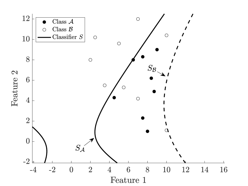
(a) Inhomogeneous quadratic kernel ($c=0.3$), $p=2$

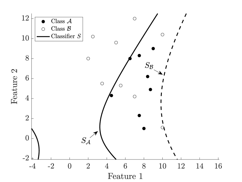
(b) Inhomogeneous quadratic kernel ($c=0.3$), $p=\infty$

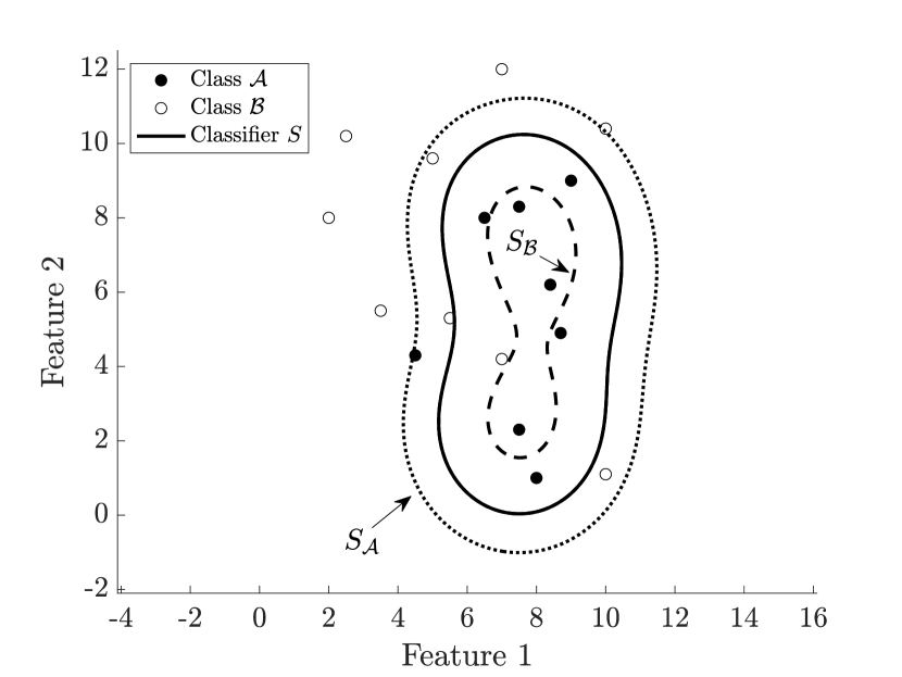
(c) Gaussian RBF kernel ($\alpha=1.9$), $p=2$

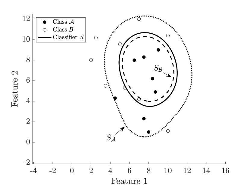
(d) Gaussian RBF kernel ($\alpha=1.9$), $p=\infty$

Figure 3: Separating surfaces obtained with inhomogeneous quadratic kernel and Gaussian RBF kernel from the robust model. The $\ell_{p}$-norms defining the uncertainty set are $p=2$ and $p=\infty$.

6 Computational results

In this section, we evaluate the performance of the deterministic model presented in Section 4 and its robust counterpart (22). The models have been implemented in MATLAB (v. 2021b) and solved using MOSEK solver (v. 9.1.9). Linear search problems (10) and (27) have been solved as in Faccini et al. (2022). Specifically, the interval $[\gamma+1-\omega_{\mathcal{B}},\gamma-1+\omega_{\mathcal{A}}]$ has been split into $10^{4}$ subintervals of equal length, and the problem is solved on each of them. The final solution is then given by the minimum value of all subproblems. All computational experiments were run on a MacBookPro17.1 with a chip Apple M1 of 8 cores and 16 GB of RAM memory.
In order to test the performance of the proposed methodology on real-world data, we perform classification experiments on a selection of datasets taken from the UCI Machine Learning Repository (see Dua and Graff (2017)). The datasets are listed in Table 3, along with the corresponding number of features $n$ and of observations $m$. As in Faccini et al. (2022), for datasets with more than two classes we adopt the one-versus-all scheme, finding the optimal classifier separating the first class of points from the remaining ones.
Each dataset is split into two disjoint parts: the training set, composed by the $\beta\%$ of the observations, and the testing set, composed by the remaining $(1-\beta)\%$. We account for three different values of $\beta$, leading to the following holdouts: 75%-25%, 50%-50%, and 25%-75%. The partition is performed inline with the proportional random sampling strategy (see Chen et al. (2001)), meaning that the original class balance in the entire dataset is maintained in both the training and testing set. Once the partition is complete, a kernel function $k(\cdot,\cdot)$ is chosen and the training set is used to train the deterministic classifier for different values of input parameter $\nu$. Specifically, as in Liu and Potra (2009) and Faccini et al. (2022), the deterministic formulation is solved on five logarithmically spaced values of $\nu$ between $10^{-3}$ and $10^{0}$. The optimal classifier is chosen among the five candidates as the one minimizing the misclassification error on the training set. Finally, the out-of-sample misclassification error on the testing set is computed, as the ratio between the total number of misclassified points in the testing set and its cardinality. This procedure is repeated 96 times, parallelizing the code on the 8 cores of the working machine, in a repeated holdout fashion (see Kim (2009)). The results are then averaged.
As far as it concerns the kernel function $k(\cdot,\cdot)$, we test seven different alternatives: homogeneous linear, homogeneous quadratic, homogeneous cubic; inhomogeneous linear, inhomogeneous quadratic, inhomogeneous cubic; Gaussian RBF. The parameter $\alpha$ in the Gaussian RBF kernel is set as the maximum value of the standard deviation across features for the dataset under consideration. Similarly for the parameter $c$ in the inhomogeneous polynomial kernels. In future works other techniques searching for the best values for hyperparameters will be explored, such as the grid-search cross validation (see Liashchynskyi and Liashchynskyi (2019)).
Potentially, the range of values in the datasets may vary widely across features, with different orders of magnitude. Since model (6) and its robust counterpart (23) are distance-based, this may result in giving high weights to specific attributes when classifying. For this reason, we apply pre-processing techniques of data transformation before training the models. Among all the possibilities we consider min-max normalization and standardization. For an overview on data pre-processing methods, the reader is referred to Han et al. (2011). On one hand, in the min-max normalization the training dataset is linearly scaled feature-wise into the $n$-dimensional hypercube $[0,1]^{n}$, according to the formula:

$$x^{(i)^{\prime}}_{j}:=\displaystyle\frac{x^{(i)}_{j}-\displaystyle\min_{l=1,\ldots,m}x^{(l)}_{j}}{\displaystyle\max_{l=1,\ldots,m}x^{(l)}_{j}-\displaystyle\min_{l=1,\ldots,m}x^{(l)}_{j}}\qquad i=1,\ldots,m,\quad j=1,\ldots,n,$$ (28)

where $x^{(i)^{\prime}}_{j}$ is the $j$-th transformed feature of observation $i$. On the other hand, in the standardization the values of a specific feature $j$ are normalized based on its mean $\mu_{j}$ and standard deviation $std_{j}$, namely:

$$x^{(i)^{\prime}}_{j}:=\displaystyle\frac{x^{(i)}_{j}-\mu_{j}}{std_{j}}\qquad i=1,\ldots,m,\quad j=1,\ldots,n.$$ (29)

In both cases, after training the deterministic model, each observation in the testing set is transformed according to the previous formulas.
Among all the optimal deterministic classifiers found for each couple data transformation-kernel function, the best configuration is chosen as the one minimizing the overall misclassification error. Within this choice of data transformation-kernel function, the robust model is solved. The bounds $\eta^{(i)}$ on the perturbation vectors defining the uncertainty sets $\mathcal{U}_{p}(x^{(i)})$ are adjusted as:

$$\eta^{(i)}=\eta_{\mathcal{A}}:=\rho_{\mathcal{A}}\max_{j=1,\ldots,n}std_{j,\mathcal{A}}\qquad\forall i:x^{(i)}\in\mathcal{A}$$

$$\eta^{(i)}=\eta_{\mathcal{B}}:=\rho_{\mathcal{B}}\max_{j=1,\ldots,n}std_{j,\mathcal{B}}\qquad\forall i:x^{(i)}\in\mathcal{B},$$

where $\rho_{\mathcal{A}}$ is a non-negative parameter allowing the user to tailor the degree of conservatism and $\displaystyle\max_{j=1,\ldots,n}std_{j,\mathcal{A}}$ is the maximum standard deviation feature-wise for training points of class $\mathcal{A}$. Similarly for $\rho_{\mathcal{B}}$ and $\displaystyle\max_{j=1,\ldots,n}std_{j,\mathcal{B}}$. For simplicity, we set $\rho_{\mathcal{A}}=\rho_{\mathcal{B}}=\rho$, and consider 7 logarithmically spaced values between $10^{-7}$ and $10^{-1}$. As in the deterministic case, we average the out-of-sample testing errors for 96 random partitions of the dataset.
For each dataset, we report in Table 3 the best configuration data transformation-kernel function, along with the average out-of-sample testing errors and standard deviations for the deterministic and robust models. We consider the three main types of uncertainty set in the literature, defined respectively by $\ell_{1}$-, $\ell_{2}$- and $\ell_{\infty}$-norm. The listed results refer to the holdout 75% training set-25% testing set. Details are reported in the B respectively in Tables 6-8 for the deterministic model, and in Tables 9-14 for the robust model.

Dataset	Data transformation	Kernel	Deterministic	Robust
$m\times n$				$p=1$	$p=2$	$p=\infty$
Arrhythmia	$-$	Gaussian RBF	$20.47\%\pm 0.07$	$\underline{\mathbf{19.12\%\pm 0.08}}$	$19.30\%\pm 0.07$	$19.61\%\pm 0.07$
$68\times 279$
CPU time (s)			0.289	0.290	0.288	0.295
Parkinson	Min-max normalization	Hom. linear	$13.19\%\pm 0.03$	$12.98\%\pm 0.03$	$\underline{\mathbf{12.37\%\pm 0.03}}$	$12.61\%\pm 0.04$
$195\times 22$
CPU time (s)			3.626	3.421	3.454	3.418
Heart Disease	Standardization	Inhom. linear	$17.48\%\pm 0.04$	$16.84\%\pm 0.04$	$17.53\%\pm 0.03$	$\underline{\mathbf{16.36\%\pm 0.04}}$
$297\times 13$
CPU time (s)			12.253	11.602	11.477	11.417
Dermatology	$-$	Inhom. quadratic	$1.64\%\pm 0.02$	$1.65\%\pm 0.01$	$1.57\%\pm 0.01$	$\underline{\mathbf{0.55\%\pm 0.01}}$
$358\times 34$
CPU time (s)			20.173	20.055	20.420	20.147
Climate Model Crashes	$-$	Hom. linear	$5.01\%\pm 0.02$	$4.47\%\pm 0.02$	$4.50\%\pm 0.01$	$\underline{\mathbf{4.34\%\pm 0.01}}$
$540\times 18$
CPU time (s)			68.069	66.762	67.169	67.381
Breast Cancer Diagnostic	Min-max normalization	Inhom. quadratic	$3.02\%\pm 0.02$	$2.63\%\pm 0.01$	$2.65\%\pm 0.01$	$\underline{\mathbf{2.56\%\pm 0.01}}$
$569\times 30$
CPU time (s)			77.786	77.968	78.267	77.543
Breast Cancer	Standardization	Hom. linear	$3.17\%\pm 0.01$	$\underline{\mathbf{2.97\%\pm 0.01}}$	$3.07\%\pm 0.01$	$3.06\%\pm 0.01$
$683\times 9$
CPU time (s)			135.765	135.651	137.039	136.286
Blood Transfusion	Standardization	Inhom. cubic	$20.72\%\pm 0.02$	$20.60\%\pm 0.02$	$\underline{\mathbf{20.55\%\pm 0.02}}$	$20.64\%\pm 0.02$
$748\times 4$
CPU time (s)			178.136	178.751	179.682	180.083
Mammographic Mass	Standardization	Inhom. quadratic	$15.71\%\pm 0.02$	$15.49\%\pm 0.02$	$\underline{\mathbf{15.42\%\pm 0.02}}$	$15.54\%\pm 0.02$
$830\times 5$
CPU time (s)			241.205	241.810	242.614	241.929

Table 3: Average out-of-sample testing errors and standard deviations over 96 runs. Holdout: 75% training set-25% testing set.

We notice that all the considered robust formulations outperform the corresponding deterministic result. Specifically, in 4 out of 9 datasets the best results are achieved by the box robust formulation ($p=\infty$), followed by the ellipsoidal ($p=2$, in 3 out of 9) and finally by the polyhedral ($p=1$). Since box uncertainty sets are the most wide around data among the three, this implies that the proposed formulation benefits from a more conservative approach when treating uncertainties.
For the sake of completeness, we explore in details the performance of the proposed models when applied to the dataset “Parkinson”. First of all, we discuss the results of the deterministic approach, with respect to both data transformation and kernel function. The out-of-sample testing errors for the holdout 75%-25% are depicted in Figure 4, while detailed results are reported in Table 6 in the B. We note that the worst performances occur when no data transformations are applied (see the dash-dotted line in Figure 4). Conversely, min-max normalization (28) and standardization (29) provide good and comparable results: the best performance is achieved by the linear kernel on min-max normalized data ($13.19\%)$. Similar conclusions can be drawn for holdouts 50%-50% and 25%-75%, where in those cases the homogeneous quadratic kernel outperforms the others, still in the case of min-max normalized data (see Tables 7-8 in B).

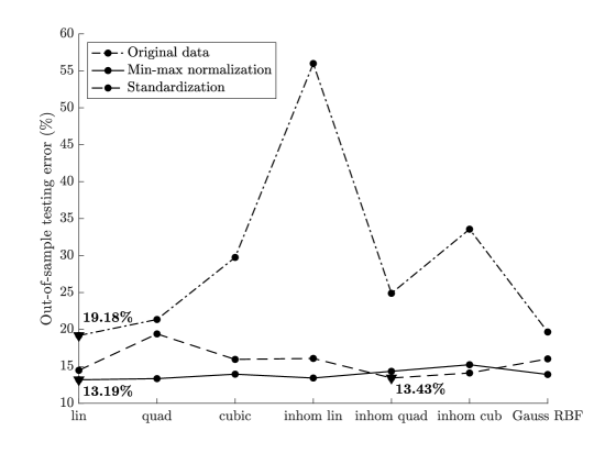
Figure 4: Out-of-sample testing error of the deterministic formulation applied to the dataset “Parkinson”. Each triangle represents the lowest error for the corresponding data transformation technique. Holdout: 75% training set-25% testing set.

In order to evaluate the performance of the robust model, we consider 60 logarithmically spaced values of $\rho$ between $10^{-7}$ and $10^{-1}$. The results are depicted in Figure 5. We notice that the increase of the value of $\beta$ leads to better performances when considering the overall out-of-sample testing error (see Figure 5(a)), since more data points in the training set are available as input of the optimization model. In addition, when perturbations are included in the model, the performances improve with respect to the deterministic case. Indeed, the great majority of the points lies below the corresponding horizontal line, representing the out-of-sample testing error of the deterministic classifier. Interestingly, the increase of the uncertainty impacts differently on the two classes (see Figure 5(b)). It can be noted that points of class $\mathcal{A}$ benefit from including high perturbations in the model. On the contrary, points of class $\mathcal{B}$ are worsen classified when the level of corruption is high.

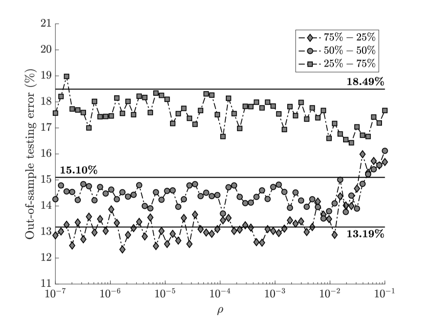
(a) Overall results.

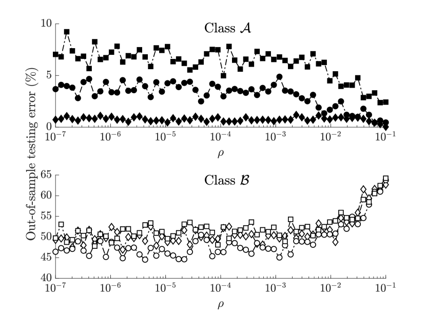
(b) Results divided by class.

Figure 5: Out-of-sample testing error of the robust formulation applied to the dataset “Parkinson”. Overall results are on the left, with the performance of the deterministic classifier depicted as horizontal line for each holdout. Results divided by class are on the right. The values of $\rho$ are in logarithmic scale.

In addition, we compare the performance of our models with the results reported in Faccini et al. (2022) and Bertsimas et al. (2019). As shown in Table 4, in 6 out of 9 datasets the results of our deterministic classifier outperform the other methods. Consequently, the linear approach presented in Liu and Potra (2009) benefits from a generalization towards nonlinear classifier. Moreover, within the same 6 datasets, our robust formulation leads to even better accuracy, implying that it is meaningful to consider uncertainties in the proposed SVM-type model.

Dataset	Deterministic			Robust
	Table 3	Faccini et al. (2022)	Bertsimas et al. (2019)	Table 3	Faccini et al. (2022)	Bertsimas et al. (2019)
Arrhythmia	$\underline{20.47\%}$	$25.65\%$	$43.08\%$	$\underline{\mathbf{19.12\%}}$	$23.00\%$	$29.23\%$
Parkinson	$\underline{13.19\%}$	$14.13\%$	$14.36\%$	$\underline{\mathbf{12.37\%}}$	$13.00\%$	$16.41\%$
Heart Disease	$17.48\%$	$16.68\%$	$\underline{\mathbf{15.93\%}}$	$16.36\%$	$\underline{16.20\%}$	$16.61\%$
Dermatology	$1.64\%$	$\underline{0.56\%}$	$3.38\%$	$0.55\%$	$\underline{\mathbf{0.13\%}}$	$1.13\%$
Climate Model Crashes	$5.01\%$	$\underline{4.99\%}$	$5.00\%$	$4.34\%$	$4.34\%$	$\underline{\mathbf{4.07\%}}$
Breast Cancer Diagnostic	$\underline{3.02\%}$	$4.89\%$	$6.49\%$	$\underline{\mathbf{2.56\%}}$	$3.89\%$	$4.04\%$
Breast Cancer	$\underline{3.17\%}$	$3.49\%$	$5.00\%$	$\underline{\mathbf{2.97\%}}$	$3.12\%$	$4.26\%$
Blood Transfusion	$\underline{20.72\%}$	$23.49\%$	$23.62\%$	$\underline{\mathbf{20.55\%}}$	$22.55\%$	$23.62\%$
Mammographic Mass	$\underline{15.71\%}$	$-$	$18.07\%$	$\underline{\mathbf{15.42\%}}$	$-$	$19.28\%$

Table 4: Out-of-sample testing error comparison among deterministic and robust results of Table 3, data from Faccini et al. (2022) and Bertsimas et al. (2019). For each approach and dataset, the best result is underlined. The lowest out-of-sample testing error within a dataset is in bold.

From Table 3 it can be noticed that the choice of the best data transformation method strongly depends on the dataset. In order to guide the final user among the three possible techniques, we report in Table 5 summary statistics on the 9 datasets. Specifically, for each feature we compute the mean and the corresponding coefficient of variation, defined as the ratio between the standard deviation and the mean. In Table 5 we list the minimum and the maximum values of the two considered indices for each dataset, along with the corresponding best data transformation. We argue that, whenever the values of the observations are close, and so the minimum and the maximum too, the best approach is to classify the original data without any transformation (see datasets “Arrhythmia”, “Dermatology” and “Climate Model Crashes”). In the extreme case of the presence of some constant features, i.e., the minimum and the maximum values coincide, and thus the coefficient of variation is null, formulas (28)-(29) cannot be applied since the denominator is equal to zero. This situation occurs with the dataset “Arrhythmia”, where only original data can be classified. On the other hand, the min-max normalization is a suitable choice when the order of magnitude across the features varies a lot. For instance, in datasets “Parkinson” and “Breast cancer diagnostic” there are 7 and 5 orders of magnitude of difference between the minimum and the maximum value of the mean of the features. Finally, standardization is an appropriate method in all other cases, where no significant differences occur among the orders of magnitude of the features (see datasets “Heart Disease”, “Breast Cancer”, “Blood Transfusion” and “Mammographic Mass”).

Dataset	Data transformation		Mean value of features	CV of features
Arrhythmia	$-$	Min	$2.23\times 10^{2}$	$0$
		Max	$6.20\times 10^{2}$	$5.29\times 10^{-1}$
Parkinson	Min-max normalization	Min	$4.40\times 10^{-5}$	$7.71\times 10^{-2}$
		Max	$1.97\times 10^{2}$	$1.63\times 10^{0}$
Heart Disease	Standardization	Min	$1.45\times 10^{-1}$	$1.35\times 10^{-1}$
		Max	$2.47\times 10^{2}$	$2.43\times 10^{0}$
Dermatology	$-$	Min	$1.06\times 10^{-1}$	$3.20\times 10^{-1}$
		Max	$3.63\times 10^{1}$	$4.29\times 10^{0}$
Climate Model Crashes	$-$	Min	$5.00\times 10^{-1}$	$5.78\times 10^{-1}$
		Max	$5.00\times 10^{-1}$	$5.78\times 10^{-1}$
Breast Cancer Diagnostic	Min-max normalization	Min	$3.79\times 10^{-3}$	$1.12\times 10^{-1}$
		Max	$8.81\times 10^{2}$	$1.13\times 10^{0}$
Breast Cancer	Standardization	Min	$1.59\times 10^{0}$	$6.41\times 10^{-1}$
		Max	$4.39\times 10^{0}$	$1.09\times 10^{0}$
Blood Transfusion	Standardization	Min	$5.51\times 10^{0}$	$7.11\times 10^{-1}$
		Max	$1.38\times 10^{3}$	$1.06\times 10^{0}$
Mammographic Mass	Standardization	Min	$2.78\times 10^{0}$	$1.59\times 10^{-1}$
		Max	$5.58\times 10^{1}$	$5.57\times 10^{-1}$

Table 5: Minimum and maximum values for the mean and the coefficient of variation (CV) computed feature-wise. The data transformation refers to the best choice when classifying the holdout 75%-25%.

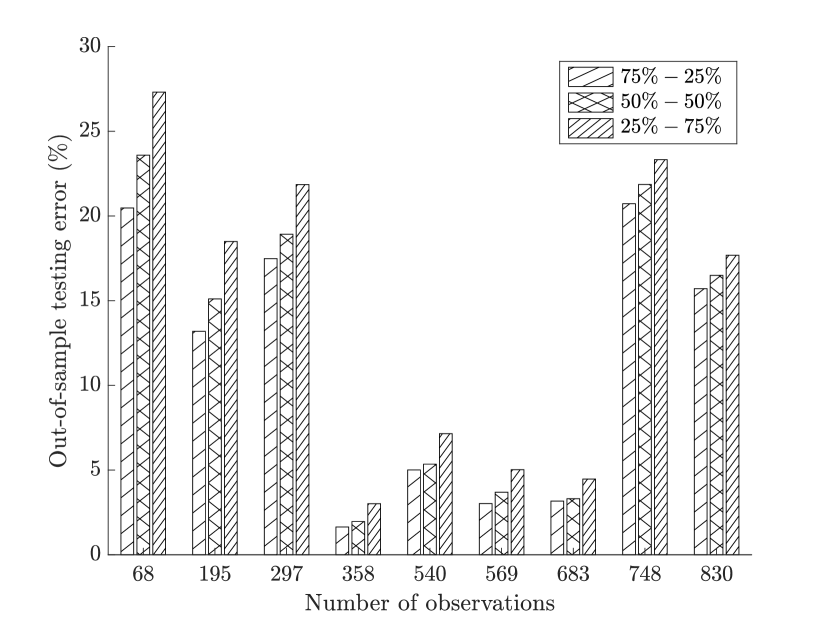
(b) Out-of-sample testing error (%).

Figure 7: Comparison between the computational time to find the best deterministic classifier and the out-of-sample testing error for the three holdouts (75%-25%, 50%-50%, 25%-75%).

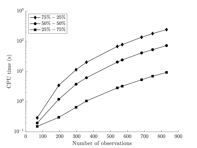
(a) Computational time (s).

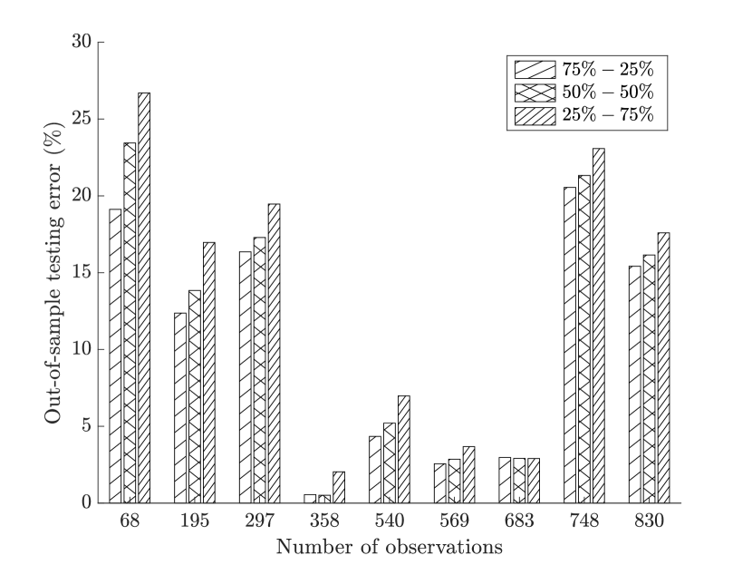
(b) Out-of-sample testing error (%).

Figure 8: Comparison between the computational time to find the best robust classifier and the out-of-sample testing error for the three holdouts (75%-25%, 50%-50%, 25%-75%).

Furthermore, in C we depict the average CPU time to find the best deterministic classifier for each dataset and for each holdout. Data are taken from Tables 6-14 in B. Numerical results show that the computational time is significantly high for datasets with a large number of observations, especially when considering 75% of the instances as training set (see Figure 7(a)). The performing speed benefits from a reduction of $\beta$, even if at the cost of worsening the accuracy. Nevertheless, as reported in Figure 7(b), when datasets are equally split in training and testing set, the accuracy does not decrease significantly compared to the case 75%-25%. A similar conclusion is valid for the robust model (see Figure 8 in C). Within this case, it can be noticed that with dataset “Dermatology” the holdout 50%-50% performs slight better than the case with 75%-25%, whereas with “Breast Cancer” the robust model has the same predictive power, regardless of the considered holdouts. Consequently, we argue that the holdout 50% training set-50% testing set can be considered as the best trade-off between accuracy and computational time for the proposed model, especially when the number of observations in the dataset is relevant.

7 Conclusions

In this paper, we have proposed a new optimization model for solving a binary classification task through SVM. From a methodological perspective, we have extended the technique studied in Liu and Potra (2009) to the nonlinear context through the introduction of a kernel function. Data are mapped from the input space to a higher-dimensional space and a final linear search procedure aiming to minimize the overall misclassification error is considered. Motivated by the uncertain nature of real-world data, we have adopted a RO approach by constructing around each input data an uncertainty set bounded-by-$\ell_{p}$-norm, with $p\in[1,\infty]$. Perturbation propagates from the input space to the feature space through the kernel function. Therefore, we have derived closed-form expressions for the uncertainty sets in the feature space, extending the results present in the literature. Finally, we have derived the robust counterpart of the deterministic model in the case of nonlinear classifier. Both the deterministic and the robust formulation reduce to LP problem, with clear advantages in terms of computational efficiency. The proposed models have been tested on real-world datasets, considering different combinations of data transformations and kernel functions. The results outperform other linear SVM approaches in most cases, even in the deterministic framework. Overall, the model benefits from including uncertainty during the training process. The accuracy is affected by the choice of the kernel function and of the data transformation before training. For this reason, we have drawn managerial insights to guide the user in choosing the best configuration.
Future research works will focus on: an extension of the proposed robust methodology with uncertainty in the labels of input data, or both in the labels and in the feature; a distributionally robust formulation with ambiguity sets defined by moments (see Wiesemann et al. (2014)) or induced by $\phi$-divergences (Duchi and Namkoong (2021)) and Wasserstein distance (Kuhn et al. (2019)); an extension to the case of multiclass classification; an application of the presented robust approach to other SVM-type models, for instance the TWSVM (Jayadeva et al. (2007)) or the TPMSVM (Peng (2011)).

References

Appendix A Supplementary proofs

Proof of Lemma 1

Proof.

We consider the two inequalities separately, starting from $\left\lVert x\right\rVert_{q}\leq\left\lVert x\right\rVert_{p}$. First of all, if $x=0$, then the inequality is obviously true. Otherwise, let $y\in\mathbb{R}^{n}$ such that $y_{i}:=\left\lvert x_{i}\right\rvert/\left\lVert x\right\rVert_{q}$ for $i=1,\ldots,n$. Therefore, $0\leq y_{i}\leq 1$. Indeed:

$$\left\lVert x\right\rVert_{q}^{q}=\sum_{i=1}^{n}\left\lvert x_{i}\right\rvert^{q}\geq\left\lvert x_{i}\right\rvert^{q},$$

for all $i=1,\ldots,n$ and thus $\left\lvert x_{i}\right\rvert/\left\lVert x\right\rVert_{q}\leq 1$. The hypothesis $p\leq q$ and the decreasing property of the exponential function with basis lower than one imply that:

$$y_{i}^{p}\geq y_{i}^{q},\qquad i=1,\ldots,n$$

and so, by summing:

$$\left\lVert y\right\rVert_{p}\geq\left\lVert y\right\rVert_{q}.$$

Finally, by definition of $y$ we derive that:

$$\frac{\left\lVert x\right\rVert_{p}}{\left\lVert x\right\rVert_{q}}\geq\frac{\left\lVert x\right\rVert_{q}}{\left\lVert x\right\rVert_{q}}=1,$$

from which the thesis follows.
On the other hand, to prove the second inequality we recall the Hölder inequality (see, for instance, Rudin (1987)). Let $a$ and $b$ be in $\mathbb{R}^{n}$. If $r$ and $r^{\prime}$ are conjugate exponents, i.e. $\textstyle\frac{1}{r}+\frac{1}{r^{\prime}}=1$, with $1\leq r,r^{\prime}\leq\infty$, then:

$$\left\lVert ab\right\rVert_{1}\leq\left\lVert a\right\rVert_{r}\cdot\left\lVert b\right\rVert_{r^{\prime}},$$

or, equivalently, in extended form:

$$\sum_{i=1}^{n}\left\lvert a_{i}\right\rvert\left\lvert b_{i}\right\rvert\leq\bigg{(}\sum_{i=1}^{n}\left\lvert a_{i}\right\rvert^{r}\bigg{)}^{\textstyle\frac{1}{r}}\cdot\bigg{(}\sum_{i=1}^{n}\left\lvert b_{i}\right\rvert^{r^{\prime}}\bigg{)}^{\textstyle\frac{1}{r^{\prime}}}.$$ (30)

First of all, we rewrite the $\ell_{p}$-norm of $x$ as:

$$\left\lVert x\right\rVert_{p}^{p}=\sum_{i=1}^{n}\left\lvert x_{i}\right\rvert^{p}=\sum_{i=1}^{n}\left\lvert x_{i}\right\rvert^{p}\cdot 1.$$

In the Hölder inequality (30), let $a=x$ and $b=e$ and consider as conjugate exponents $r=\textstyle\frac{q}{p}$ and $r^{\prime}=\textstyle\frac{q}{q-p}$. Both $r$ and $r^{\prime}$ are greater than or equal to 1 because, by hypothesis, $p\leq q$. Consequently, we can bound the $\ell_{p}$-norm of $x$ by:

$$\begin{split}\left\lVert x\right\rVert_{p}^{p}&\leq\bigg{(}\sum_{i=1}^{n}\big{(}\left\lvert x_{i}\right\rvert^{p}\big{)}^{\textstyle\frac{q}{p}}\bigg{)}^{\textstyle\frac{p}{q}}\cdot\bigg{(}\sum_{i=1}^{n}1^{\textstyle\frac{q}{q-p}}\bigg{)}^{1-\textstyle\frac{p}{q}}\\ &=\bigg{(}\sum_{i=1}^{n}\left\lvert x_{i}\right\rvert^{q}\bigg{)}^{\textstyle\frac{p}{q}}n^{1-\textstyle\frac{p}{q}}\\ &=\left\lVert x\right\rVert_{q}^{p}n^{1-\textstyle\frac{p}{q}}.\end{split}$$

Finally, the thesis follows by taking the $p$-th root of both sides of the inequality. ∎

A graphical representation of inequality (13) is depicted in Figure 6.

Figure 6: Graphical representation of the thesis of Lemma 1 in the case of $p=1.3$, $q=2$, $n=2$. The dashed $\ell_{2}$ unit ball lies between the $\ell_{1.3}$ unit ball and the $\ell_{1.3}$ ball with radius $2^{\frac{1}{1.3}-\frac{1}{2}}\approx 1.205$.

Proof of Lemma 2

Proof.

By definition of the inhomogeneous polynomial kernel of degree $d$, the last right-hand side of (17) becomes:

$$\begin{split}\left\lVert\zeta^{(i)}\right\rVert^{2}_{\mathcal{H}}&=\bigg{(}\left\lVert x^{(i)}+\sigma^{(i)}\right\rVert^{2}_{2}+c\bigg{)}^{d}-2\big{(}\langle x^{(i)}+\sigma^{(i)},x^{(i)}\rangle+c\big{)}^{d}+\bigg{(}\left\lVert x^{(i)}\right\rVert^{2}_{2}+c\bigg{)}^{d}\\ &=\bigg{(}\left\lVert x^{(i)}\right\rVert_{2}^{2}+\left\lVert\sigma^{(i)}\right\rVert_{2}^{2}+2\text{ }\langle\sigma^{(i)},x^{(i)}\rangle+c\bigg{)}^{d}+\\ &\quad-2\bigg{(}\left\lVert x^{(i)}\right\rVert_{2}^{2}+\langle\sigma^{(i)},x^{(i)}\rangle+c\bigg{)}^{d}+\bigg{(}\left\lVert x^{(i)}\right\rVert^{2}_{2}+c\bigg{)}^{d}.\end{split}$$

If we apply the Cauchy-Schwarz inequality in $\mathbb{R}^{n}$ to the terms containing the dot product, the previous expression simplifies further, leading to:

$$\begin{split}\left\lVert\zeta^{(i)}\right\rVert^{2}_{\mathcal{H}}&\leq\bigg{(}\left\lVert x^{(i)}\right\rVert_{2}^{2}+\left\lVert\sigma^{(i)}\right\rVert_{2}^{2}+2\left\lVert\sigma^{(i)}\right\rVert_{2}\left\lVert x^{(i)}\right\rVert_{2}+c\bigg{)}^{d}+\\ &\quad-2\bigg{(}\left\lVert x^{(i)}\right\rVert_{2}^{2}+\left\lVert\sigma^{(i)}\right\rVert_{2}\left\lVert x^{(i)}\right\rVert_{2}+c\bigg{)}^{d}+\bigg{(}\left\lVert x^{(i)}\right\rVert_{2}^{2}+c\bigg{)}^{d}\\ &=\bigg{[}\bigg{(}\left\lVert x^{(i)}\right\rVert_{2}+\left\lVert\sigma^{(i)}\right\rVert_{2}\bigg{)}^{2}+c\bigg{]}^{d}+\\ &\quad-2\bigg{[}\left\lVert x^{(i)}\right\rVert_{2}\bigg{(}\left\lVert x^{(i)}\right\rVert_{2}+\left\lVert\sigma^{(i)}\right\rVert_{2}\bigg{)}+c\bigg{]}^{d}+\bigg{(}\left\lVert x^{(i)}\right\rVert_{2}^{2}+c\bigg{)}^{d}.\end{split}$$

The binomial theorem applied to three $d$-th powers implies that:

$$\begin{split}\left\lVert\zeta^{(i)}\right\rVert^{2}_{\mathcal{H}}&\leq\sum_{k=0}^{d}\binom{d}{k}c^{k}\bigg{(}\left\lVert x^{(i)}\right\rVert_{2}+\left\lVert\sigma^{(i)}\right\rVert_{2}\bigg{)}^{2(d-k)}+\\ &\quad-2\sum_{k=0}^{d}\binom{d}{k}c^{k}\left\lVert x^{(i)}\right\rVert_{2}^{d-k}\bigg{(}\left\lVert x^{(i)}\right\rVert_{2}+\left\lVert\sigma^{(i)}\right\rVert_{2}\bigg{)}^{d-k}+\\ &\quad+\sum_{k=0}^{d}\binom{d}{k}c^{k}\left\lVert x^{(i)}\right\rVert_{2}^{2(d-k)}.\end{split}$$

We now split all the three sums by considering separately the cases when $k=0$, $k=d$ and, then, all the intermediate cases. Firstly, let us call $a_{0}$ the addendum of the sum corresponding to $k=0$. Therefore:

$$\begin{split}a_{0}&=\bigg{(}\left\lVert x^{(i)}\right\rVert_{2}+\left\lVert\sigma^{(i)}\right\rVert_{2}\bigg{)}^{2d}-2\left\lVert x^{(i)}\right\rVert_{2}^{d}\bigg{(}\left\lVert x^{(i)}\right\rVert_{2}+\left\lVert\sigma^{(i)}\right\rVert_{2}\bigg{)}^{d}+\left\lVert x^{(i)}\right\rVert_{2}^{2d}\\ &=\bigg{[}\bigg{(}\left\lVert x^{(i)}\right\rVert_{2}+\left\lVert\sigma^{(i)}\right\rVert_{2}\bigg{)}^{d}-\left\lVert x^{(i)}\right\rVert_{2}^{d}\bigg{]}^{2}\\ &=\bigg{[}\sum_{k=0}^{d}\binom{d}{k}\left\lVert x^{(i)}\right\rVert^{d-k}_{2}\left\lVert\sigma^{(i)}\right\rVert_{2}^{k}-\left\lVert x^{(i)}\right\rVert_{2}^{d}\bigg{]}^{2}\\ &=\bigg{[}\sum_{k=1}^{d}\binom{d}{k}\left\lVert x^{(i)}\right\rVert^{d-k}_{2}\left\lVert\sigma^{(i)}\right\rVert_{2}^{k}+\left\lVert x^{(i)}\right\rVert_{2}^{d}-\left\lVert x^{(i)}\right\rVert_{2}^{d}\bigg{]}^{2}\\ &=\bigg{[}\sum_{k=1}^{d}\binom{d}{k}\left\lVert x^{(i)}\right\rVert^{d-k}_{2}\left\lVert\sigma^{(i)}\right\rVert_{2}^{k}\bigg{]}^{2}.\end{split}$$

We notice that $a_{0}$ is the only addendum of the sum that does not contain $c$. This implies that $a_{0}$ is related to the bound $\delta^{(i)}$ for the homogeneous polynomial kernel.
Secondly, if $k=d$, we have no contribution because:

$$c^{d}-2c^{d}+c^{d}=0.$$

Before considering the cases $k=1,\ldots,d-1$, we now investigate what happens when the degree $d$ is equal to 1. Here, the index $k$ of the sums goes from 0 to 1, and therefore, as seen before:

$$\left\lVert\zeta^{(i)}\right\rVert^{2}_{\mathcal{H}}\leq\big{(}\delta^{(i)}_{\text{hom}}\big{)}^{2}=\big{(}C\eta^{(i)}\big{)}^{2}.$$

Hence, when $d=1$, then:

$$\delta^{(i)}=C\eta^{(i)}.$$

Conversely, when $d>1$, we have all the addenda between $k=1$ and $k=d-1$. Thus, by combining all the three sums together accordingly to the previous observations, we have:

$$\begin{split}\left\lVert\zeta^{(i)}\right\rVert^{2}_{\mathcal{H}}&\leq a_{0}+\sum_{k=1}^{d-1}\binom{d}{k}c^{k}\bigg{[}\bigg{(}\left\lVert x^{(i)}\right\rVert_{2}+\left\lVert\sigma^{(i)}\right\rVert_{2}\bigg{)}^{2(d-k)}+\\ &\quad-2\left\lVert x^{(i)}\right\rVert_{2}^{d-k}\bigg{(}\left\lVert x^{(i)}\right\rVert_{2}+\left\lVert\sigma^{(i)}\right\rVert_{2}\bigg{)}^{d-k}+\left\lVert x^{(i)}\right\rVert_{2}^{2(d-k)}\bigg{]}\\ &=a_{0}+\sum_{k=1}^{d-1}\binom{d}{k}c^{k}\bigg{[}\bigg{(}\left\lVert x^{(i)}\right\rVert_{2}+\left\lVert\sigma^{(i)}\right\rVert_{2}\bigg{)}^{d-k}-\left\lVert x^{(i)}\right\rVert_{2}^{d-k}\bigg{]}^{2}.\end{split}$$

Again, by applying the binomial theorem to the $(d-k)$-th power of $\big{(}\left\lVert x^{(i)}\right\rVert_{2}+\left\lVert\sigma^{(i)}\right\rVert_{2}\big{)}$ and by splitting the sum, we are able to simplify the last term. Hence:

$$\begin{split}\left\lVert\zeta^{(i)}\right\rVert^{2}_{\mathcal{H}}&\leq a_{0}+\sum_{k=1}^{d-1}\binom{d}{k}c^{k}\bigg{[}\sum_{j=0}^{d-k}\binom{d-k}{j}\left\lVert x^{(i)}\right\rVert_{2}^{d-k-j}\left\lVert\sigma^{(i)}\right\rVert_{2}^{j}-\left\lVert x^{(i)}\right\rVert_{2}^{d-k}\bigg{]}^{2}\\ &=a_{0}+\sum_{k=1}^{d-1}\binom{d}{k}c^{k}\bigg{[}\sum_{j=1}^{d-k}\binom{d-k}{j}\left\lVert x^{(i)}\right\rVert_{2}^{d-k-j}\left\lVert\sigma^{(i)}\right\rVert_{2}^{j}\bigg{]}^{2}.\end{split}$$

Therefore, by taking the square root:

$$\left\lVert\zeta^{(i)}\right\rVert_{\mathcal{H}}\leq\sqrt{a_{0}+\sum_{k=1}^{d-1}\binom{d}{k}c^{k}\bigg{[}\sum_{j=1}^{d-k}\binom{d-k}{j}\left\lVert x^{(i)}\right\rVert_{2}^{d-k-j}\left\lVert\sigma^{(i)}\right\rVert_{2}^{j}\bigg{]}^{2}}.$$

According to inequalities (14)$-$(15) and to hypothesis $\left\lVert\sigma^{(i)}\right\rVert_{p}\leq\eta^{(i)}$, we obtain that:

$$\left\lVert\sigma^{(i)}\right\rVert_{2}\leq\left\{\begin{array}[]{ll}\left\lVert\sigma^{(i)}\right\rVert_{p}\leq\eta^{(i)},&1\leq p\leq 2\\ \\ n^{\textstyle\frac{p-2}{2p}}\left\lVert\sigma^{(i)}\right\rVert_{p}\leq n^{\textstyle\frac{p-2}{2p}}\eta^{(i)},&p>2.\end{array}\right.$$

Finally, whenever $1\leq p\leq 2$, we have that:

$$\begin{split}a_{0}&\leq\bigg{[}\sum_{k=1}^{d}\binom{d}{k}\left\lVert x^{(i)}\right\rVert^{d-k}_{2}\left\lVert\sigma^{(i)}\right\rVert_{p}^{k}\bigg{]}^{2}\\ &\leq\bigg{[}\sum_{k=1}^{d}\binom{d}{k}\left\lVert x^{(i)}\right\rVert^{d-k}_{2}\big{(}\eta^{(i)}\big{)}^{k}\bigg{]}^{2}=\big{(}\delta^{(i)}_{\text{hom}}\big{)}^{2},\end{split}$$

and the second addendum in the square root can be bounded by:

$$\sum_{k=1}^{d-1}\binom{d}{k}c^{k}\bigg{[}\sum_{j=1}^{d-k}\binom{d-k}{j}\left\lVert x^{(i)}\right\rVert_{2}^{d-k-j}\big{(}\eta^{(i)}\big{)}^{j}\bigg{]}^{2}.$$

On the other hand, if $p>2$, then:

$$\begin{split}a_{0}&\leq\bigg{[}\sum_{k=1}^{d}\binom{d}{k}\left\lVert x^{(i)}\right\rVert^{d-k}_{2}n^{\textstyle\frac{k(p-2)}{2p}}\left\lVert\sigma^{(i)}\right\rVert_{p}^{k}\bigg{]}^{2}\\ &\leq\bigg{[}\sum_{k=1}^{d}\binom{d}{k}\left\lVert x^{(i)}\right\rVert^{d-k}_{2}\bigg{(}n^{\textstyle\frac{p-2}{2p}}\eta^{(i)}\bigg{)}^{k}\bigg{]}^{2}=\big{(}\delta^{(i)}_{\text{hom}}\big{)}^{2},\end{split}$$

and similarly the second addendum in the square root is always less than or equal to:

$$\sum_{k=1}^{d-1}\binom{d}{k}c^{k}\bigg{[}\sum_{j=1}^{d-k}\binom{d-k}{j}\left\lVert x^{(i)}\right\rVert_{2}^{d-k-j}\bigg{(}n^{\textstyle\frac{p-2}{2p}}\eta^{(i)}\bigg{)}^{j}\bigg{]}^{2}.$$

∎

Proof of Lemma 3

Proof.

For all $x$ in $\mathbb{R}^{n}$, we have that $k(x,x)=1$ and, thus, equation (17) reduces to:

$$\begin{split}\left\lVert\zeta^{(i)}\right\rVert^{2}_{\mathcal{H}}&=1-2\exp\bigg{(}\displaystyle-\frac{\left\lVert x^{(i)}+\sigma^{(i)}-x^{(i)}\right\rVert^{2}_{2}}{2\alpha^{2}}\bigg{)}+1\\ &=2-2\exp\bigg{(}\displaystyle-\frac{\left\lVert\sigma^{(i)}\right\rVert^{2}_{2}}{2\alpha^{2}}\bigg{)}.\end{split}$$

Therefore:

$$\left\lVert\zeta^{(i)}\right\rVert_{\mathcal{H}}=\sqrt{2-2\exp\bigg{(}\displaystyle-\frac{\left\lVert\sigma^{(i)}\right\rVert^{2}_{2}}{2\alpha^{2}}\bigg{)}}.$$

The thesis follows by applying inequalities (14)$-$(15) and by considering the monotonicity of function $g(x)=-\exp(-x^{2})$ when $x>0$.

∎

Appendix B Supplementary results

Dataset	Data transformation	Kernel
		Hom. linear	Hom. quadratic	Hom. cubic	Inhom. linear	Inhom. quadratic	Inhom. cubic	Gaussian RBF
Arrhythmia	$-$	$21.94\%\pm 0.10$	$53.43\%\pm 0.20$	$-$	$21.88\%\pm 0.10$	$53.31\%\pm 0.20$	$-$	$\underline{\mathbf{20.47\%\pm 0.07}}$
	CPU time (s)	0.298	0.297	$-$	0.309	0.290	$-$	0.289
	Min-max normalization	$-$	$-$	$-$	$-$	$-$	$-$	$-$
	CPU time (s)	$-$	$-$	$-$	$-$	$-$	$-$	$-$
	Standardization	$-$	$-$	$-$	$-$	$-$	$-$	$-$
	CPU time (s)	$-$	$-$	$-$	$-$	$-$	$-$	$-$
Parkinson	$-$	$\underline{19.18\%\pm 0.10}$	$21.35\%\pm 0.06$	$29.75\%\pm 0.15$	$55.99\%\pm 0.36$	$24.89\%\pm 0.12$	$33.57\%\pm 0.18$	$19.66\%\pm 0.03$
	CPU time (s)	3.698	3.661	4.402	3.713	3.762	4.259	3.702
	Min-max normalization	$\underline{\mathbf{13.19\%\pm 0.03}}$	$13.35\%\pm 0.04$	$13.95\%\pm 0.05$	$13.43\%\pm 0.05$	$14.34\%\pm 0.05$	$15.23\%\pm 0.04$	$13.91\%\pm 0.04$
	CPU time (s)	3.626	3.657	3.636	3.731	3.754	3.656	3.629
	Standardization	$14.47\%\pm 0.04$	$19.40\%\pm 0.06$	$15.95\%\pm 0.06$	$16.08\%\pm 0.06$	$\underline{13.43\%\pm 0.05}$	$14.11\%\pm 0.05$	$16.02\%\pm 0.05$
	CPU time (s)	3.621	3.542	3.600	3.640	3.628	3.673	3.576
Heart Disease	$-$	$\underline{23.47\%\pm 0.09}$	$27.79\%\pm 0.05$	$37.36\%\pm 0.08$	$35.28\%\pm 0.13$	$29.77\%\pm 0.08$	$40.37\%\pm 0.09$	$33.01\%\pm 0.05$
	CPU time (s)	12.102	12.646	13.050	12.296	12.391	12.755	12.333
	Min-max normalization	$18.57\%\pm 0.04$	$19.82\%\pm 0.04$	$22.75\%\pm 0.05$	$\underline{18.01\%\pm 0.04}$	$19.75\%\pm 0.04$	$22.24\%\pm 0.05$	$31.84\%\pm 0.06$
	CPU time (s)	12.115	12.167	12.050	12.124	12.061	12.162	12.749
	Standardization	$19.00\%\pm 0.04$	$37.27\%\pm 0.06$	$23.56\%\pm 0.04$	$\underline{\mathbf{17.48\%\pm 0.04}}$	$27.48\%\pm 0.05$	$24.07\%\pm 0.04$	$47.49\%\pm 0.04$
	CPU time (s)	12.162	12.100	12.203	12.253	12.532	12.123	11.597
Dermatology	$-$	$5.41\%\pm 0.06$	$2.05\%\pm 0.01$	$3.03\%\pm 0.02$	$6.14\%\pm 0.07$	$\underline{\mathbf{1.64\%\pm 0.02}}$	$2.90\%\pm 0.02$	$7.81\%\pm 0.08$
	CPU time (s)	20.584	20.032	19.969	20.094	20.091	20.033	20.246
	Min-max normalization	$3.35\%\pm 0.03$	$2.84\%\pm 0.02$	$\underline{1.85\%\pm 0.01}$	$3.34\%\pm 0.03$	$3.02\%\pm 0.02$	$1.95\%\pm 0.02$	$30.83\%\pm 0.01$
	CPU time (s)	20.253	20.329	20.173	20.102	20.178	20.132	20.548
	Standardization	$\underline{3.23\%\pm 0.03}$	$5.59\%\pm 0.03$	$3.29\%\pm 0.02$	$3.86\%\pm 0.03$	$5.22\%\pm 0.03$	$3.35\%\pm 0.02$	$30.83\%\pm 0.01$
	CPU time (s)	20.050	20.118	20.290	20.073	20.127	20.230	20.349
Climate Model Crashes	$-$	$\underline{\mathbf{5.01\%\pm 0.02}}$	$6.04\%\pm 0.02$	$8.23\%\pm 0.02$	$5.25\%\pm 0.02$	$5.87\%\pm 0.02$	$7.64\%\pm 0.02$	$13.19\%\pm 0.03$
	CPU time (s)	68.069	67.104	65.726	66.070	65.745	66.235	66.383
	Min-max normalization	$\underline{5.08\%\pm 0.02}$	$5.52\%\pm 0.02$	$7.78\%\pm 0.02$	$5.09\%\pm 0.02$	$5.87\%\pm 0.02$	$7.82\%\pm 0.03$	$13.50\%\pm 0.03$
	CPU time (s)	68.296	68.102	69.397	68.228	68.510	69.750	70.330
	Standardization	$5.20\%\pm 0.02$	$20.15\%\pm 0.03$	$11.54\%\pm 0.02$	$\underline{5.11\%\pm 0.02}$	$15.73\%\pm 0.04$	$11.57\%\pm 0.03$	$13.81\%\pm 0.03$
	CPU time (s)	67.022	66.851	66.544	65.792	65.528	65.046	69.635
Breast Cancer Diagnostic	$-$	$10.69\%\pm 0.15$	$24.85\%\pm 0.22$	$-$	$16.06\%\pm 0.21$	$41.46\%\pm 0.23$	$-$	$\underline{8.58\%\pm 0.02}$
	CPU time (s)	76.706	77.126	$-$	76.718	78.570	$-$	80.493
	Min-max normalization	$4.12\%\pm 0.03$	$3.15\%\pm 0.02$	$3.88\%\pm 0.02$	$4.39\%\pm 0.03$	$\underline{\mathbf{3.02\%\pm 0.02}}$	$5.80\%\pm 0.05$	$12.87\%\pm 0.05$
	CPU time (s)	76.340	76.476	76.106	76.350	77.786	78.282	77.690
	Standardization	$\underline{3.65\%\pm 0.02}$	$17.72\%\pm 0.03$	$5.40\%\pm 0.02$	$3.88\%\pm 0.02$	$6.88\%\pm 0.02$	$4.92\%\pm 0.02$	$36.62\%\pm 0.01$
	CPU time (s)	78.100	78.279	77.534	76.813	76.041	76.715	77.248
Breast Cancer	$-$	$3.21\%\pm 0.01$	$7.02\%\pm 0.02$	$8.36\%\pm 0.07$	$3.39\%\pm 0.02$	$6.84\%\pm 0.02$	$11.58\%\pm 0.16$	$\underline{3.20\%\pm 0.01}$
	CPU time (s)	133.833	132.231	133.750	134.134	134.697	135.338	133.728
	Min-max normalization	$4.06\%\pm 0.04$	$3.29\%\pm 0.01$	$4.20\%\pm 0.02$	$4.12\%\pm 0.02$	$4.43\%\pm 0.03$	$4.82\%\pm 0.02$	$\underline{3.20\%\pm 0.01}$
	CPU time (s)	135.390	135.382	135.109	137.616	136.871	134.736	136.484
	Standardization	$\underline{\mathbf{3.17\%\pm 0.01}}$	$6.80\%\pm 0.03$	$5.88\%\pm 0.02$	$3.19\%\pm 0.01$	$6.21\%\pm 0.02$	$5.61\%\pm 0.02$	$3.88\%\pm 0.02$
	CPU time (s)	135.765	135.553	136.774	135.623	134.514	135.597	137.221
Blood Transfusion	$-$	$24.09\%\pm 0.01$	$26.57\pm 0.15$	$-$	$24.00\%\pm 0.01$	$27.35\%\pm 0.15$	$-$	$\underline{23.73\%\pm 0.01}$
	CPU time (s)	170.744	176.855	$-$	174.407	176.929	$-$	174.808
	Min-max normalization	$23.82\%\pm 0.00$	$23.85\%\pm 0.01$	$23.73\%\pm 0.02$	$23.84\%\pm 0.00$	$23.92\%\pm 0.01$	$\underline{23.25\%\pm 0.01}$	$23.53\%\pm 0.02$
	CPU time (s)	176.273	178.011	178.221	177.326	179.052	175.440	176.455
	Standardization	$23.85\%\pm 0.01$	$23.37\%\pm 0.01$	$22.00\%\pm 0.02$	$24.01\%\pm 0.01$	$20.97\%\pm 0.02$	$\underline{\mathbf{20.72\%\pm 0.02}}$	$21.09\%\pm 0.02$
	CPU time (s)	178.088	178.107	177.398	177.692	179.141	178.136	176.627
Mammographic Mass	$-$	$20.92\%\pm 0.07$	$\underline{15.85\%\pm 0.02}$	$17.51\%\pm 0.05$	$17.12\%\pm 0.02$	$16.20\%\pm 0.02$	$28.47\%\pm 0.15$	$18.48\%\pm 0.02$
	CPU time (s)	240.550	239.300	241.644	241.607	242.298	242.582	239.141
	Min-max normalization	$26.22\%\pm 0.12$	$16.60\%\pm 0.02$	$16.09\%\pm 0.02$	$26.77\%\pm 0.13$	$\underline{16.04\%\pm 0.02}$	$16.06\%\pm 0.02$	$17.25\%\pm 0.02$
	CPU time (s)	241.645	240.950	239.648	241.134	241.525	239.143	241.536
	Standardization	$19.49\%\pm 0.06$	$31.14\%\pm 0.05$	$18.82\%\pm 0.03$	$19.73\%\pm 0.08$	$\underline{\mathbf{15.71\%\pm 0.02}}$	$18.63\%\pm 0.02$	$18.29\%\pm 0.02$
	CPU time (s)	239.300	236.677	239.877	238.003	241.205	242.163	240.254

Table 6: Detailed results of average out-of-sample testing errors and standard deviations over 96 runs of the deterministic model. Holdout: 75% training set-25% testing set.

Dataset	Data transformation	Kernel
		Hom. linear	Hom. quadratic	Hom. cubic	Inhom. linear	Inhom. quadratic	Inhom. cubic	Gaussian RBF
Arrhythmia	$-$	$23.90\%\pm 0.06$	$54.23\%\pm 0.02$	$-$	$24.08\%\pm 0.05$	$51.72\%\pm 0.21$	$-$	$\underline{\mathbf{23.59\%\pm 0.04}}$
	CPU time (s)	0.194	0.180	$-$	0.191	0.216	$-$	0.181
	Min-max normalization	$-$	$-$	$-$	$-$	$-$	$-$	$-$
	CPU time (s)	$-$	$-$	$-$	$-$	$-$	$-$	$-$
	Standardization	$-$	$-$	$-$	$-$	$-$	$-$	$-$
	CPU time (s)	$-$	$-$	$-$	$-$	$-$	$-$	$-$
Parkinson	$-$	$\underline{19.58\%\pm 0.11}$	$25.10\%\pm 0.06$	$40.05\%\pm 0.22$	$46.88\%\pm 0.27$	$23.70\%\pm 0.07$	$32.07\%\pm 0.17$	$19.97\%\pm 0.05$
	CPU time (s)	1.283	1.230	1.290	1.211	1.330	1.382	1.264
	Min-max normalization	$15.54\%\pm 0.06$	$\underline{\mathbf{15.10\%\pm 0.04}}$	$16.02\%\pm 0.04$	$15.43\%\pm 0.04$	$16.26\%\pm 0.04$	$16.13\%\pm 0.04$	$18.38\%\pm 0.04$
	CPU time (s)	1.195	1.203	1.206	1.214	1.202	1.207	1.184
	Standardization	$\underline{15.79\%\pm 0.04}$	$22.71\%\pm 0.06$	$17.74\%\pm 0.05$	$17.62\%\pm 0.04$	$17.98\%\pm 0.04$	$17.71\%\pm 0.05$	$19.33\%\pm 0.05$
	CPU time (s)	1.203	1.257	1.207	1.201	1.193	1.204	1.183
Heart Disease	$-$	$\underline{23.00\%\pm 0.08}$	$28.55\%\pm 0.04$	$37.81\%\pm 0.07$	$31.07\%\pm 0.13$	$30.36\%\pm 0.07$	$42.13\%\pm 0.09$	$34.45\%\pm 0.04$
	CPU time (s)	4.132	4.199	4.732	4.193	4.223	4.821	4.045
	Min-max normalization	$20.00\%\pm 0.03$	$21.40\%\pm 0.03$	$22.87\%\pm 0.04$	$20.11\%\pm 0.06$	$20.82\%\pm 0.03$	$22.64\%\pm 0.03$	$32.07\%\pm 0.06$
	CPU time (s)	4.078	4.076	4.097	4.063	4.098	4.168	4.057
	Standardization	$19.05\%\pm 0.04$	$37.16\%\pm 0.04$	$23.97\%\pm 0.03$	$\underline{\mathbf{18.92\%\pm 0.03}}$	$26.82\%\pm 0.04$	$23.99\%\pm 0.04$	$46.01\%\pm 0.04$
	CPU time (s)	4.182	4.131	4.147	4.138	4.075	4.112	4.095
Dermatology	$-$	$8.90\%\pm 0.08$	$2.01\%\pm 0.01$	$3.17\%\pm 0.02$	$12.08\%\pm 0.11$	$\underline{\mathbf{1.96\%\pm 0.01}}$	$3.34\%\pm 0.02$	$8.82\%\pm 0.08$
	CPU time (s)	5.999	6.015	6.115	6.089	6.075	6.072	6.115
	Min-max normalization	$4.35\%\pm 0.05$	$3.45\%\pm 0.02$	$2.55\%\pm 0.02$	$4.82\%\pm 0.06$	$3.93\%\pm 0.02$	$\underline{2.42\%\pm 0.01}$	$30.97\%\pm 0.00$
	CPU time (s)	6.019	6.159	6.049	6.077	6.090	6.021	6.137
	Standardization	$4.16\%\pm 0.03$	$7.16\%\pm 0.02$	$4.19\%\pm 0.02$	$4.78\%\pm 0.03$	$5.74\%\pm 0.02$	$\underline{4.14\%\pm 0.02}$	$30.97\%\pm 0.00$
	CPU time (s)	6.092	6.127	6.258	6.137	6.146	6.101	6.101
Climate Model Crashes	$-$	$5.56\%\pm 0.01$	$7.01\%\pm 0.02$	$8.16\%\pm 0.02$	$\underline{\mathbf{5.35\%\pm 0.01}}$	$7.44\%\pm 0.02$	$8.23\%\pm 0.02$	$13.42\%\pm 0.02$
	CPU time (s)	20.032	20.018	20.056	20.035	20.051	20.145	19.856
	Min-max normalization	$5.57\%\pm 0.01$	$7.21\%\pm 0.02$	$8.24\%\pm 0.02$	$\underline{5.42\%\pm 0.01}$	$7.17\%\pm 0.02$	$8.29\%\pm 0.02$	$13.57\%\pm 0.02$
	CPU time (s)	20.742	21.174	20.553	20.941	20.628	20.147	20.740
	Standardization	$\underline{5.82\%\pm 0.01}$	$20.01\%\pm 0.03$	$11.77\%\pm 0.02$	$6.40\%\pm 0.02$	$15.21\%\pm 0.03$	$11.55\%\pm 0.03$	$13.14\%\pm 0.02$
	CPU time (s)	20.059	19.566	19.518	19.702	19.748	19.780	20.310
Breast Cancer Diagnostic	$-$	$13.53\%\pm 0.18$	$27.06\%\pm 0.24$	$-$	$16.94\%\pm 0.23$	$34.81\%\pm 0.23$	$-$	$\underline{9.26\%\pm 0.02}$
	CPU time (s)	24.553	24.289	$-$	24.410	24.671	$-$	24.525
	Min-max normalization	$6.21\%\pm 0.06$	$3.87\%\pm 0.03$	$4.43\%\pm 0.01$	$5.99\%\pm 0.05$	$\underline{\mathbf{3.69\%\pm 0.02}}$	$5.19\%\pm 0.03$	$20.68\%\pm 0.08$
	CPU time (s)	24.449	24.405	24.600	24.671	24.237	24.634	23.636
	Standardization	$\underline{4.17\%\pm 0.02}$	$19.01\%\pm 0.02$	$5.67\%\pm 0.02$	$4.45\%\pm 0.03$	$7.43\%\pm 0.02$	$5.22\%\pm 0.01$	$37.21\%\pm 0.00$
	CPU time (s)	24.472	24.526	24.855	24.664	22.988	23.080	23.791
Breast Cancer	$-$	$4.54\%\pm 0.04$	$6.47\%\pm 0.02$	$12.57\%\pm 0.11$	$\underline{3.61\%\pm 0.02}$	$6.72\%\pm 0.01$	$26.05\%\pm 0.25$	$3.84\%\pm 0.01$
	CPU time (s)	39.279	39.238	40.161	38.794	40.341	39.618	39.730
	Min-max normalization	$5.71\%\pm 0.06$	$\underline{\mathbf{3.31\%\pm 0.01}}$	$4.52\%\pm 0.01$	$10.05\%\pm 0.11$	$4.37\%\pm 0.02$	$4.99\%\pm 0.01$	$3.62\%\pm 0.01$
	CPU time (s)	38.718	40.067	39.394	39.775	39.780	39.395	42.094
	Standardization	$\underline{3.37\%\pm 0.01}$	$7.69\%\pm 0.02$	$6.13\%\pm 0.01$	$3.75\%\pm 0.01$	$6.43\%\pm 0.01$	$5.97\%\pm 0.01$	$5.08\%\pm 0.02$
	CPU time (s)	38.914	39.175	38.866	39.353	39.007	38.892	40.610
Blood Transfusion	$-$	$23.81\%\pm 0.01$	$\underline{22.99\%\pm 0.01}$	$-$	$23.68\%\pm 0.00$	$31.60\%\pm 0.19$	$-$	$25.40\%\pm 0.09$
	CPU time (s)	49.452	50.652	$-$	51.609	54.469	$-$	51.579
	Min-max normalization	$23.85\%\pm 0.00$	$23.84\%\pm 0.01$	$23.69\%\pm 0.01$	$23.81\%\pm 0.00$	$23.77\%\pm 0.01$	$23.59\%\pm 0.01$	$\underline{23.38\%\pm 0.01}$
	CPU time (s)	51.422	51.582	52.451	52.365	51.648	52.098	51.996
	Standardization	$23.77\%\pm 0.01$	$23.77\%\pm 0,01$	$22.52\%\pm 0.01$	$23.69\%\pm 0.00$	$21.98\%\pm 0.01$	$\underline{\mathbf{21.86\%\pm 0.03}}$	$22.07\%\pm 0.01$
	CPU time (s)	51.396	52.654	53.843	52.609	52.676	52.658	52.006
Mammographic Mass	$-$	$24.02\%\pm 0.10$	$\underline{17.28\%\pm 0.05}$	$35.66\%\pm 0.16$	$25.55\%\pm 0.11$	$40.95\%\pm 0.14$	$46.42\%\pm 0.09$	$19.84\pm 0.02$
	CPU time (s)	70.958	70.916	71.854	71.198	72.179	72.495	70.880
	Min-max normalization	$21.74\%\pm 0.09$	$17.72\%\pm 0.02$	$\underline{\mathbf{16.49\%\pm 0.02}}$	$23.36\%\pm 0.11$	$19.71\%\pm 0.08$	$18.62\%\pm 0.08$	$17.94\%\pm 0.01$
	CPU time (s)	71.468	71.291	71.426	71.415	71.274	73.143	71.589
	Standardization	$20.08\%\pm 0.06$	$32.87\%\pm 0.07$	$19.86\%\pm 0.02$	$20.25\%\pm 0.06$	$\underline{16.56\%\pm 0.01}$	$19.54\%\pm 0.02$	$18.84\%\pm 0.02$
	CPU time (s)	70.693	72.523	72.951	71.156	71.861	71.803	71.269

Table 7: Detailed results of average out-of-sample testing errors and standard deviations over 96 runs of the deterministic model. Holdout: 50% training set-50% testing set.

Dataset	Data transformation	Kernel
		Hom. linear	Hom. quadratic	Hom. cubic	Inhom. linear	Inhom. quadratic	Inhom. cubic	Gaussian RBF
Arrhythmia	$-$	$28.66\%\pm 0.07$	$53.45\%\pm 0.20$	$-$	$\underline{\mathbf{27.31\%\pm 0.07}}$	$53.84\%\pm 0.20$	$-$	$28.29\%\pm 0.02$
	CPU time (s)	0.142	0.165	$-$	0.144	0.148	$-$	0.153
	Min-max normalization	$-$	$-$	$-$	$-$	$-$	$-$	$-$
	CPU time (s)	$-$	$-$	$-$	$-$	$-$	$-$	$-$
	Standardization	$-$	$-$	$-$	$-$	$-$	$-$	$-$
	CPU time (s)	$-$	$-$	$-$	$-$	$-$	$-$	$-$
Parkinson	$-$	$26.58\%\pm 0.17$	$25.55\%\pm 0.05$	$45.19\%\pm 0.24$	$37.54\%\pm 0.25$	$25.85\%\pm 0.08$	$45.44\%\pm 0.25$	$\underline{21.48\%\pm 0.03}$
	CPU time (s)	0.293	0.303	0.530	0.301	0.285	0.596	0.295
	Min-max normalization	$18.91\%\pm 0.05$	$\underline{\mathbf{18.49\%\pm 0.04}}$	$20.92\%\pm 0.05$	$19.98\%\pm 0.06$	$19.66\%\pm 0.07$	$21.08\%\pm 0.06$	$21.88\%\pm 0.04$
	CPU time (s)	0.311	0.286	0.281	0.291	0.294	0.301	0.291
	Standardization	$20.03\%\pm 0.04$	$30.18\%\pm 0.05$	$23.10\%\pm 0.06$	$\underline{19.73\%\pm 0.04}$	$23.47\%\pm 0.06$	$22.85\%\pm 0.05$	$23.78\%\pm 0.05$
	CPU time (s)	0.286	0.292	0.278	0.277	0.289	0.301	0.289
Heart Disease	$-$	$\underline{25.58\%\pm 0.08}$	$28.73\%\pm 0.04$	$42.38\%\pm 0.08$	$28.03\%\pm 0.10$	$29.50\%\pm 0.06$	$46.02\%\pm 0.08$	$36.61\%\pm 0.04$
	CPU time (s)	0.656	0.648	1.496	0.703	0.682	1.863	0.613
	Min-max normalization	$22.00\%\pm 0.05$	$23.18\%\pm 0.03$	$22.76\%\pm 0.03$	$\underline{\mathbf{21.85\%\pm 0.05}}$	$23.33\%\pm 0.04$	$23.07\%\pm 0.03$	$38.86\%\pm 0.07$
	CPU time (s)	0.638	0.640	0.663	0.625	0.628	0.640	0.634
	Standardization	$\underline{22.48\%\pm 0.04}$	$39.13\%\pm 0.04$	$25.48\%\pm 0.04$	$22.94\%\pm 0.06$	$28.38\%\pm 0.03$	$25.67\%\pm 0.04$	$45.74\%\pm 0.03$
	CPU time (s)	0.640	0.653	0.701	0.637	0.629	0.623	0.629
Dermatology	$-$	$13.17\%\pm 0.11$	$\underline{3.13\%\pm 0.02}$	$4.19\%\pm 0.03$	$13.88\%\pm 0.11$	$3.14\%\pm 0.02$	$4.18\%\pm 0.04$	$10.01\%\pm 0.04$
	CPU time (s)	0.971	0.981	0.963	0.956	0.951	0.965	0.974
	Min-max normalization	$10.32\%\pm 0.11$	$5.81\%\pm 0.05$	$3.65\%\pm 0.02$	$9.03\%\pm 0.10$	$5.66\%\pm 0.05$	$\underline{\mathbf{3.01\%\pm 0.02}}$	$30.97\%\pm 0.00$
	CPU time (s)	1.006	1.100	0.958	0.960	0.960	0.977	0.957
	Standardization	$\underline{6.74\%\pm 0.04}$	$10.54\%\pm 0.03$	$7.35\%\pm 0.03$	$7.97\%\pm 0.05$	$9.52\%\pm 0.03$	$7.05\%\pm 0.03$	$30.97\%\pm 0.00$
	CPU time (s)	0.968	0.962	0.957	0.953	0.972	0.967	0.955
Climate Model Crashes	$-$	$7.28\%\pm 0.01$	$10.51\%\pm 0.02$	$10.47\%\pm 0.02$	$\underline{\mathbf{7.15\%\pm 0.01}}$	$10.59\%\pm 0.03$	$11.18\%\pm 0.03$	$14.34\%\pm 0.02$
	CPU time (s)	2.804	2.715	2.686	2.671	2.653	2.662	2.811
	Min-max normalization	$\underline{7.20\%\pm 0.01}$	$10.54\%\pm 0.02$	$10.80\%\pm 0.03$	$7.27\%\pm 0.01$	$10.77\%\pm 0.03$	$10.66\%\pm 0.03$	$14.14\%\pm 0.02$
	CPU time (s)	2.847	2.827	2.840	2.848	2.865	2.856	2.839
	Standardization	$10.04\%\pm 0.03$	$19.74\%\pm 0.05$	$12.58\%\pm 0.04$	$\underline{9.99\%\pm 0.03}$	$14.36\%\pm 0.04$	$12.53\%\pm 0.03$	$13.51\%\pm 0.02$
	CPU time (s)	2.874	2.823	2.759	2.844	2.853	2.814	2.827
Breast Cancer Diagnostic	$-$	$17.25\%\pm 0.19$	$39.75\%\pm 0.24$	$-$	$20.31\%\pm 0.23$	$28.03\%\pm 0.23$	$-$	$\underline{11.21\%\pm 0.04}$
	CPU time (s)	3.498	3.515	$-$	3.256	3.419	$-$	3.376
	Min-max normalization	$8.62\%\pm 0.07$	$6.29\%\pm 0.05$	$5.98\%\pm 0.02$	$8.89\%\pm 0.08$	$\underline{5.87\%\pm 0.04}$	$6.43\%\pm 0.03$	$33.15\%\pm 0.06$
	CPU time (s)	3.439	3.249	3.285	3.289	3.250	3.255	3.395
	Standardization	$5.11\%\pm 0.02$	$22.85\%\pm 0.03$	$6.37\%\pm 0.02$	$\underline{\mathbf{5.02\%\pm 0.02}}$	$10.49\%\pm 0.02$	$6.17\%\pm 0.02$	$37.32\%\pm 0.00$
	CPU time (s)	3.287	3.309	3.317	3.278	3.381	3.302	3.278
Breast Cancer	$-$	$7.05\%\pm 0.06$	$6.58\%\pm 0.02$	$21.30\%\pm 0.14$	$6.56\%\pm 0.06$	$6.73\%\pm 0.02$	$21.95\%\pm 0.20$	$\underline{5.00\%\pm 0.02}$
	CPU time (s)	5.392	5.318	5.406	5.440	5.490	5.506	5.511
	Min-max normalization	$8.62\%\pm 0.09$	$\underline{\mathbf{4.47\%\pm 0.02}}$	$5.92\%\pm 0.02$	$11.70\%\pm 0.11$	$5.01\%\pm 0.04$	$5.83\%\pm 0.02$	$5.00\%\pm 0.02$
	CPU time (s)	5.507	5.536	5.574	5.420	5.463	5.522	5.505
	Standardization	$5.12\%\pm 0.05$	$9.45\%\pm 0.02$	$6.36\%\pm 0.02$	$\underline{4.64\%\pm 0.03}$	$7.33\%\pm 0.02$	$6.18\%\pm 0.02$	$6.01\%\pm 0.02$
	CPU time (s)	5.526	5.423	5.399	5.413	5.418	5.422	5.565
Blood Transfusion	$-$	$23.69\%\pm 0.00$	$\underline{23.55\%\pm 0.01}$	$-$	$23.69\%\pm 0.01$	$42.69\%\pm 0.25$	$-$	$23.96\%\pm 0.01$
	CPU time (s)	7.214	7.618	$-$	7.342	7.622	$-$	6.838
	Min-max normalization	$23.85\%\pm 0.01$	$23.75\%\pm 0.01$	$23.69\%\pm 0.01$	$23.77\%\pm 0.00$	$23.68\%\pm 0.00$	$23.68\%\pm 0.01$	$\underline{23.53\%\pm 0.01}$
	CPU time (s)	7.319	7.430	7.141	7.398	7.122	7.144	6.665
	Standardization	$23.75\%\pm 0.01$	$23.63\%\pm 0.00$	$\underline{\mathbf{23.32\%\pm 0.01}}$	$23.72\%\pm 0.00$	$23.37\%\pm 0.05$	$26.03\%\pm 0.09$	$23.35\%\pm 0.01$
	CPU time (s)	7.357	7.145	7.222	7.183	7.084	7.344	6.737
Mammographic Mass	$-$	$28.35\%\pm 0.13$	$\underline{18.83\%\pm 0.05}$	$37.40\%\pm 0.14$	$30.20\%\pm 0.14$	$36.33\%\pm 0.15$	$39.55\%\pm 0.15$	$22.21\%\pm 0.03$
	CPU time (s)	9.024	9.013	9.166	9.206	9.152	9.166	8.964
	Min-max normalization	$22.21\%\pm 0.09$	$19.02\%\pm 0.04$	$\underline{\mathbf{17.68\%\pm 0.02}}$	$24.31\%\pm 0.11$	$19.56\%\pm 0.05$	$20.38\%\pm 0.08$	$19.39\%\pm 0.02$
	CPU time (s)	9.068	9.086	9.116	9.019	9.009	9.021	8.953
	Standardization	$19.48\%\pm 0.04$	$32.89\%\pm 0.09$	$21.98\%\pm 0.04$	$21.02\%\pm 0.06$	$\underline{19.21\%\pm 0.04}$	$24.04\%\pm 0.07$	$20.13\%\pm 0.02$
	CPU time (s)	9.114	9.125	9.184	9.101	9.152	9.250	9.114

Table 8: Detailed results of average out-of-sample testing errors and standard deviations over 96 runs of the deterministic model. Holdout: 25% training set-75% testing set.

Dataset	Data transformation	Kernel	$\rho$	Robust
				$p=1$	$p=2$	$p=\infty$
Arrhythmia	$-$	Gaussian RBF	$10^{-7}$	$19.18\%\pm 0.07$	$19.42\%\pm 0.07$	$19.67\%\pm 0.07$
			$10^{-6}$	$19.30\%\pm 0.06$	$19.61\%\pm 0.07$	$20.40\%\pm 0.08$
			$10^{-5}$	$20.47\%\pm 0.07$	$19.91\%\pm 0.07$	$19.73\%\pm 0.06$
			$10^{-4}$	$20.10\%\pm 0.07$	$19.55\%\pm 0.07$	$\underline{19.61\%\pm 0.07}$
			$10^{-3}$	$\underline{\mathbf{19.12\%\pm 0.08}}$	$\underline{19.30\%\pm 0.07}$	$23.28\%\pm 0.06$
			$10^{-2}$	$19.30\%\pm 0.07$	$20.83\%\pm 0.08$	$29.41\%\pm 0.00$
			$10^{-1}$	$29.41\%\pm 0.00$	$29.41\%\pm 0.00$	$29.41\%\pm 0.00$
			CPU time (s)	0.290	0.288	0.295
Parkinson	Min-max normalization	Hom. linear	$10^{-7}$	$\underline{12.98\%\pm 0.03}$	$12.87\%\pm 0.03$	$13.02\%\pm 0.04$
			$10^{-6}$	$13.50\%\pm 0.04$	$13.02\%\pm 0.04$	$12.80\%\pm 0.04$
			$10^{-5}$	$13.04\%\pm 0.04$	$13.28\%\pm 0.04$	$\underline{12.61\%\pm 0.04}$
			$10^{-4}$	$13.93\%\pm 0.03$	$\underline{\mathbf{12.37\%\pm 0.03}}$	$12.72\%\pm 0.03$
			$10^{-3}$	$13.54\%\pm 0.03$	$13.32\%\pm 0.04$	$13.48\%\pm 0.04$
			$10^{-2}$	$12.98\%\pm 0.03$	$13.17\%\pm 0.04$	$15.15\%\pm 0.04$
			$10^{-1}$	$15.28\%\pm 0.03$	$15.58\%\pm 0.03$	$25.00\%\pm 0.00$
			CPU time (s)	3.421	3.454	3.418
Heart disease	Standardization	Inhom. linear	$10^{-7}$	$\underline{16.84\%\pm 0.04}$	$17.53\%\pm 0.04$	$16.84\%\pm 0.04$
			$10^{-6}$	$17.53\%\pm 0.04$	$17.72\%\pm 0.04$	$17.53\%\pm 0.04$
			$10^{-5}$	$17.37\%\pm 0.04$	$18.26\%\pm 0.03$	$17.38\%\pm 0.04$
			$10^{-4}$	$17.75\%\pm 0.04$	$18.27\%\pm 0.04$	$17.64\%\pm 0.04$
			$10^{-3}$	$17.13\%\pm 0.04$	$18.43\%\pm 0.04$	$17.12\%\pm 0.04$
			$10^{-2}$	$17.10\%\pm 0.04$	$17.92\%\pm 0.04$	$\underline{\mathbf{16.36\%\pm 0.04}}$
			$10^{-1}$	$16.98\%\pm 0.04$	$\underline{17.53\%\pm 0.03}$	$16.37\%\pm 0.04$
			CPU time (s)	11.602	11.477	11.417
Dermatology	$-$	Inhom. quadratic	$10^{-7}$	$\underline{1.65\%\pm 0.01}$	$1.71\%\pm 0.01$	$1.72\%\pm 0.01$
			$10^{-6}$	$1.78\%\pm 0.01$	$1.80\%\pm 0.02$	$1.79\%\pm 0.01$
			$10^{-5}$	$1.73\%\pm 0.02$	$\underline{1.57\%\pm 0.01}$	$1.76\%\pm 0.01$
			$10^{-4}$	$11.06\%\pm 0.04$	$0.39\%\pm 0.04$	$1.28\%\pm 0.01$
			$10^{-3}$	$30.93\%\pm 0.01$	$30.93\%\pm 0.01$	$\underline{\mathbf{0.55\%\pm 0.01}}$
			$10^{-2}$	$30.91\%\pm 0.01$	$30.86\%\pm 0.01$	$30.89\%\pm 0.01$
			$10^{-1}$	$38.06\%\pm 0.21$	$32.33\%\pm 0.10$	$30.92\%\pm 0.01$
			CPU time (s)	20.055	20.420	20.147
Climate Model Crashes	$-$	Hom. linear	$10^{-7}$	$4.74\%\pm 0.02$	$4.51\%\pm 0.01$	$4.60\%\pm 0.02$
			$10^{-6}$	$4.70\%\pm 0.02$	$4.88\%\pm 0.01$	$4.93\%\pm 0.02$
			$10^{-5}$	$4.52\%\pm 0.02$	$4.56\%\pm 0.01$	$4.71\%\pm 0.02$
			$10^{-4}$	$4.86\%\pm 0.02$	$4.78\%\pm 0.02$	$4.85\%\pm 0.01$
			$10^{-3}$	$\underline{4.47\%\pm 0.02}$	$4.71\%\pm 0.01$	$\underline{\mathbf{4.34\%\pm 0.01}}$
			$10^{-2}$	$4.67\%\pm 0.01$	$\underline{4.50\%\pm 0.01}$	$4.81\%\pm 0.02$
			$10^{-1}$	$8.46\%\pm 0.00$	$8.52\%\pm 0.00$	$8.47\%\pm 0.00$
			CPU time (s)	66.762	67.169	67.381

Table 9: Average out-of-sample testing errors and standard deviations over 96 runs of the robust model. Holdout: 75% training set-25% testing set.

Dataset	Data transformation	Kernel	$\rho$	Robust
				$p=1$	$p=2$	$p=\infty$
Breast Cancer Diagnostic	Min-max normalization	Inhom. quadratic	$10^{-7}$	$2.80\%\pm 0.01$	$\underline{2.65\%\pm 0.01}$	$2.80\%\pm 0.01$
			$10^{-6}$	$2.96\%\pm 0.02$	$2.70\%\pm 0.01$	$2.96\%\pm 0.02$
			$10^{-5}$	$\underline{2.63\%\pm 0.01}$	$2.99\%\pm 0.01$	$2.66\%\pm 0.01$
			$10^{-4}$	$2.88\%\pm 0.01$	$2.88\%\pm 0.01$	$\underline{\mathbf{2.56\%\pm 0.01}}$
			$10^{-3}$	$2.91\%\pm 0.01$	$3.19\%\pm 0.01$	$9.76\%\pm 0.03$
			$10^{-2}$	$37.32\%\pm 0.00$	$37.32\%\pm 0.00$	$37.32\%\pm 0.00$
			$10^{-1}$	$37.32\%\pm 0.00$	$37.32\%\pm 0.00$	$37.32\%\pm 0.00$
			CPU time (s)	77.968	78.267	77.543
Breast Cancer	Standardization	Hom. linear	$10^{-7}$	$3.20\%\pm 0.01$	$3.24\%\pm 0.01$	$3.17\%\pm 0.01$
			$10^{-6}$	$3.16\%\pm 0.01$	$3.26\%\pm 0.01$	$3.17\%\pm 0.01$
			$10^{-5}$	$\underline{\mathbf{2.97\%\pm 0.01}}$	$3.32\%\pm 0.01$	$3.14\%\pm 0.01$
			$10^{-4}$	$3.23\%\pm 0.01$	$3.50\%\pm 0.01$	$3.20\%\pm 0.01$
			$10^{-3}$	$3.11\%\pm 0.01$	$\underline{3.07\%\pm 0.01}$	$3.21\%\pm 0.01$
			$10^{-2}$	$3.33\%\pm 0.01$	$3.19\%\pm 0.01$	$3.08\%\pm 0.01$
			$10^{-1}$	$3.07\%\pm 0.01$	$3.32\%\pm 0.01$	$\underline{3.06\%\pm 0.01}$
			CPU time (s)	135.651	137.039	136.286
Blood Transfusion	Standardization	Inhom. cubic	$10^{-7}$	$\underline{20.60\%\pm 0.02}$	$\underline{\mathbf{20.55\%\pm 0.02}}$	$\underline{20.64\%\pm 0.02}$
			$10^{-6}$	$20.72\%\pm 0.02$	$20.80\%\pm 0.02$	$20.77\%\pm 0.02$
			$10^{-5}$	$21.26\%\pm 0.02$	$20.97\%\pm 0.02$	$22.49\%\pm 0.02$
			$10^{-4}$	$23.88\%\pm 0.00$	$23.85\%\pm 0.00$	$23.79\%\pm 0.00$
			$10^{-3}$	$23.80\%\pm 0.00$	$24.57\%\pm 0.08$	$26.18\%\pm 0.13$
			$10^{-2}$	$26.19\%\pm 0.13$	$30.94\%\pm 0.22$	$38.88\%\pm 0.31$
			$10^{-1}$	$61.12\%\pm 0.38$	$57.13\%\pm 0.38$	$56.37\%\pm 0.38$
			CPU time (s)	178.751	179.682	180.083
Mammographic Mass	Standardization	Inhom. quadratic	$10^{-7}$	$15.71\%\pm 0.02$	$\underline{\mathbf{15.42\%\pm 0.02}}$	$\underline{15.54\%\pm 0.02}$
			$10^{-6}$	$15.57\%\pm 0.02$	$15.46\%\pm 0.03$	$15.74\%\pm 0.03$
			$10^{-5}$	$\underline{15.49\%\pm 0.02}$	$16.16\%\pm 0.03$	$15.66\%\pm 0.02$
			$10^{-4}$	$15.91\%\pm 0.02$	$16.16\%\pm 0.03$	$18.81\%\pm 0.02$
			$10^{-3}$	$48.54\%\pm 0.00$	$48.56\%\pm 0.00$	$48.56\%\pm 0.00$
			$10^{-2}$	$48.57\%\pm 0.00$	$48.53\%\pm 0.00$	$48.53\%\pm 0.00$
			$10^{-1}$	$48.56\%\pm 0.00$	$48.54\%\pm 0.00$	$48.54\%\pm 0.00$
			CPU time (s)	241.810	242.614	241.929

Table 10: Average out-of-sample testing errors and standard deviations over 96 runs of the robust model. Holdout: 75% training set-25% testing set (continued).

Dataset	Data transformation	Kernel	$\rho$	Robust
				$p=1$	$p=2$	$p=\infty$
Arrhythmia	$-$	Gaussian RBF	$10^{-7}$	$24.66\%\pm 0.04$	$23.99\%\pm 0.05$	$\underline{\mathbf{23.44\%\pm 0.04}}$
			$10^{-6}$	$24.11\%\pm 0.05$	$24.63\%\pm 0.04$	$23.77\%\pm 0.05$
			$10^{-5}$	$23.81\%\pm 0.05$	$24.08\%\pm 0.04$	$24.11\%\pm 0.05$
			$10^{-4}$	$\underline{23.77\%\pm 0.05}$	$\underline{23.74\%\pm 0.05}$	$24.33\%\pm 0.05$
			$10^{-3}$	$24.51\%\pm 0.04$	$24.60\%\pm 0.05$	$26.10\%\pm 0.04$
			$10^{-2}$	$24.36\%\pm 0.04$	$23.77\%\pm 0.05$	$29.41\%\pm 0.00$
			$10^{-1}$	$29.41\%\pm 0.00$	$29.41\%\pm 0.00$	$29.41\%\pm 0.00$
			CPU time (s)	0.191	0.195	0.196
Parkinson	Min-max normalization	Hom. quadratic	$10^{-7}$	$13.92\%\pm 0.03$	$14.89\%\pm 0.04$	$14.51\%\pm 0.03$
			$10^{-6}$	$14.85\%\pm 0.03$	$14.45\%\pm 0.03$	$14.25\%\pm 0.03$
			$10^{-5}$	$14.52\%\pm 0.03$	$14.45\%\pm 0.03$	$14.45\%\pm 0.03$
			$10^{-4}$	$14.28\%\pm 0.04$	$14.28\%\pm 0.03$	$14.33\%\pm 0.03$
			$10^{-3}$	$14.84\%\pm 0.03$	$14.41\%\pm 0.03$	$\underline{13.85\%\pm 0.03}$
			$10^{-2}$	$\underline{\mathbf{13.84\%\pm 0.03}}$	$\underline{13.86\%\pm 0.03}$	$15.01\%\pm 0.03$
			$10^{-1}$	$15.38\%\pm 0.02$	$15.70\%\pm 0.02$	$24.74\%\pm 0.00$
			CPU time (s)	1.195	1.217	1.224
Heart disease	Standardization	Inhom. linear	$10^{-7}$	$18.38\%\pm 0.03$	$18.21\%\pm 0.02$	$18.21\%\pm 0.02$
			$10^{-6}$	$18.18\%\pm 0.03$	$18.53\%\pm 0.03$	$18.53\%\pm 0.03$
			$10^{-5}$	$17.98\%\pm 0.03$	$18.17\%\pm 0.03$	$18.17\%\pm 0.03$
			$10^{-4}$	$18.29\%\pm 0.03$	$18.82\%\pm 0.03$	$18.78\%\pm 0.03$
			$10^{-3}$	$18.88\%\pm 0.03$	$18.19\%\pm 0.03$	$18.19\%\pm 0.03$
			$10^{-2}$	$18.92\%\pm 0.03$	$18.22\%\pm 0.03$	$18.05\%\pm 0.03$
			$10^{-1}$	$\underline{17.34\%\pm 0.02}$	$\underline{17.65\%\pm 0.02}$	$\underline{\mathbf{17.29\%\pm 0.02}}$
			CPU time (s)	3.686	3.795	3.766
Dermatology	$-$	Inhom. quadratic	$10^{-7}$	$1.97\%\pm 0.01$	$2.19\%\pm 0.01$	$1.97\%\pm 0.01$
			$10^{-6}$	$1.93\%\pm 0.01$	$1.96\%\pm 0.01$	$1.93\%\pm 0.01$
			$10^{-5}$	$1.98\%\pm 0.01$	$2.38\%\pm 0.01$	$1.94\%\pm 0.01$
			$10^{-4}$	$2.04\%\pm 0.01$	$2.12\%\pm 0.01$	$1.71\%\pm 0.01$
			$10^{-3}$	$1.55\%\pm 0.01$	$1.40\%\pm 0.01$	$\underline{0.73\%\pm 0.01}$
			$10^{-2}$	$\underline{0.62\%\pm 0.01}$	$\underline{\mathbf{0.51\%\pm 0.01}}$	$31.00\%\pm 0.00$
			$10^{-1}$	$31.02\%\pm 0.00$	$30.98\%\pm 0.00$	$31.02\%\pm 0.00$
			CPU time (s)	6.156	6.178	6.200
Climate Model Crashes	$-$	Inhom. linear	$10^{-7}$	$5.27\%\pm 0.01$	$5.23\%\pm 0.01$	$5.23\%\pm 0.01$
			$10^{-6}$	$\underline{5.23\%\pm 0.01}$	$5.27\%\pm 0.01$	$5.27\%\pm 0.01$
			$10^{-5}$	$5.35\%\pm 0.01$	$5.35\%\pm 0.01$	$5.34\%\pm 0.01$
			$10^{-4}$	$5.46\%\pm 0.01$	$5.28\%\pm 0.01$	$\underline{5.23\%\pm 0.01}$
			$10^{-3}$	$5.43\%\pm 0.01$	$\underline{\mathbf{5.21\%\pm 0.01}}$	$5.41\%\pm 0.01$
			$10^{-2}$	$5.46\%\pm 0.01$	$5.44\%\pm 0.01$	$6.30\%\pm 0.01$
			$10^{-1}$	$8.51\%\pm 0.00$	$8.52\%\pm 0.00$	$8.52\%\pm 0.00$
			CPU time (s)	19.874	20.420	19.868

Table 11: Average out-of-sample testing errors and standard deviations over 96 runs of the robust model. Holdout: 50% training set-50% testing set.

Dataset	Data transformation	Kernel	$\rho$	Robust
				$p=1$	$p=2$	$p=\infty$
Breast Cancer Diagnostic	Min-max normalization	Inhom. quadratic	$10^{-7}$	$3.06\%\pm 0.01$	$3.19\%\pm 0.01$	$3.06\%\pm 0.01$
			$10^{-6}$	$3.19\%\pm 0.01$	$3.19\%\pm 0.01$	$3.18\%\pm 0.01$
			$10^{-5}$	$\underline{2.87\%\pm 0.01}$	$3.17\%\pm 0.01$	$\underline{\mathbf{2.86\%\pm 0.01}}$
			$10^{-4}$	$3.26\%\pm 0.01$	$\underline{2.99\%\pm 0.01}$	$3.21\%\pm 0.01$
			$10^{-3}$	$2.90\%\pm 0.01$	$3.29\%\pm 0.01$	$5.67\%\pm 0.01$
			$10^{-2}$	$11.14\%\pm 0.03$	$10.74\%\pm 0.03$	$37.32\%\pm 0.00$
			$10^{-1}$	$37.32\%\pm 0.00$	$37.32\%\pm 0.00$	$37.32\%\pm 0.00$
			CPU time (s)	23.844	24.039	24.074
Breast Cancer	Min-max normalization	Hom. quadratic	$10^{-7}$	$3.32\%\pm 0.01$	$3.32\%\pm 0.01$	$3.32\%\pm 0.01$
			$10^{-6}$	$3.22\%\pm 0.01$	$3.22\%\pm 0.01$	$3.22\%\pm 0.01$
			$10^{-5}$	$3.36\%\pm 0.01$	$3.36\%\pm 0.01$	$3.36\%\pm 0.01$
			$10^{-4}$	$3.27\%\pm 0.01$	$3.27\%\pm 0.01$	$3.23\%\pm 0.01$
			$10^{-3}$	$3.29\%\pm 0.01$	$3.29\%\pm 0.01$	$3.26\%\pm 0.01$
			$10^{-2}$	$3.24\%\pm 0.01$	$3.24\%\pm 0.01$	$3.16\%\pm 0.01$
			$10^{-1}$	$\underline{3.09\%\pm 0.01}$	$\underline{3.09\%\pm 0.01}$	$\underline{\mathbf{2.91\%\pm 0.01}}$
			CPU time (s)	40.660	40.554	41.035
Blood Transfusion	Standardization	Inhom. cubic	$10^{-7}$	$21.61\%\pm 0.01$	$\underline{21.47\%\pm 0.01}$	$21.46\%\pm 0.02$
			$10^{-6}$	$\underline{21.54\%\pm 0.02}$	$21.48\%\pm 0.02$	$\underline{\mathbf{21.33\%\pm 0.02}}$
			$10^{-5}$	$21.63\%\pm 0.01$	$21.63\%\pm 0.01$	$22.09\%\pm 0.01$
			$10^{-4}$	$23.69\%\pm 0.00$	$23.67\%\pm 0.00$	$23.80\%\pm 0.00$
			$10^{-3}$	$23.80\%\pm 0.00$	$23.80\%\pm 0.00$	$23.80\%\pm 0.00$
			$10^{-2}$	$25.38\%\pm 0.11$	$25.38\%\pm 0.11$	$30.94\%\pm 0.22$
			$10^{-1}$	$47.61\%\pm 0.36$	$47.61\%\pm 0.36$	$52.37\%\pm 0.37$
			CPU time (s)	52.918	52.915	52.598
Mammographic Mass	Min-max normalization	Hom. cubic	$10^{-7}$	$16.58\%\pm 0.02$	$16.31\%\pm 0.02$	$16.58\%\pm 0.02$
			$10^{-6}$	$16.46\%\pm 0.01$	$\underline{\mathbf{16.15\%\pm 0.01}}$	$\underline{16.46\%\pm 0.01}$
			$10^{-5}$	$16.51\%\pm 0.02$	$16.67\%\pm 0.01$	$16.54\%\pm 0.02$
			$10^{-4}$	$\underline{16.45\%\pm 0.02}$	$16.39\%\pm 0.01$	$16.54\%\pm 0.01$
			$10^{-3}$	$17.34\%\pm 0.02$	$16.84\%\pm 0.02$	$17.86\%\pm 0.02$
			$10^{-2}$	$18.05\%\pm 0.02$	$18.30\%\pm 0.02$	$18.87\%\pm 0.02$
			$10^{-1}$	$19.86\%\pm 0.01$	$19.93\%\pm 0.01$	$19.50\%\pm 0.01$
			CPU time (s)	71.626	71.648	71.730

Table 12: Average out-of-sample testing errors and standard deviations over 96 runs of the robust model. Holdout: 50% training set-50% testing set (continued).

Dataset	Data transformation	Kernel	$\rho$	Robust
				$p=1$	$p=2$	$p=\infty$
Arrhythmia	$-$	Inhom. linear	$10^{-7}$	$\underline{\mathbf{26.70\%\pm 0.07}}$	$27.47\%\pm 0.06$	$28.82\%\pm 0.06$
			$10^{-6}$	$28.00\%\pm 0.06$	$\underline{27.21\%\pm 0.06}$	$28.15\%\pm 0.07$
			$10^{-5}$	$28.66\%\pm 0.06$	$28.29\%\pm 0.06$	$28.10\%\pm 0.06$
			$10^{-4}$	$28.78\%\pm 0.06$	$28.04\%\pm 0.06$	$\underline{27.84\%\pm 0.07}$
			$10^{-3}$	$27.41\%\pm 0.06$	$28.68\%\pm 0.07$	$32.29\%\pm 0.06$
			$10^{-2}$	$31.56\%\pm 0.07$	$30.43\%\pm 0.07$	$29.41\%\pm 0.00$
			$10^{-1}$	$29.45\%\pm 0.00$	$29.45\%\pm 0.00$	$29.41\%\pm 0.00$
			CPU time (s)	0.151	0.161	0.142
Parkinson	Min-max normalization	Hom. quadratic	$10^{-7}$	$18.87\%\pm 0.04$	$18.00\%\pm 0.04$	$17.73\%\pm 0.04$
			$10^{-6}$	$18.37\%\pm 0.04$	$17.23\%\pm 0.04$	$18.12\%\pm 0.04$
			$10^{-5}$	$18.77\%\pm 0.04$	$17.84\%\pm 0.04$	$18.15\%\pm 0.04$
			$10^{-4}$	$17.65\%\pm 0.04$	$17.18\%\pm 0.04$	$17.62\%\pm 0.04$
			$10^{-3}$	$17.43\%\pm 0.04$	$17.46\%\pm 0.04$	$17.93\%\pm 0.04$
			$10^{-2}$	$\underline{\mathbf{16.96\%\pm 0.04}}$	$\underline{17.18\%\pm 0.04}$	$\underline{17.07\%\pm 0.03}$
			$10^{-1}$	$17.04\%\pm 0.03$	$17.22\%\pm 0.03$	$24.66\%\pm 0.00$
			CPU time (s)	0.301	0.304	0.303
Heart disease	Min-max normalization	Inhom. linear	$10^{-7}$	$19.99\%\pm 0.03$	$20.39\%\pm 0.03$	$20.97\%\pm 0.03$
			$10^{-6}$	$20.93\%\pm 0.03$	$20.59\%\pm 0.03$	$21.17\%\pm 0.03$
			$10^{-5}$	$20.91\%\pm 0.03$	$20.88\%\pm 0.03$	$20.97\%\pm 0.03$
			$10^{-4}$	$20.51\%\pm 0.03$	$20.25\%\pm 0.03$	$20.49\%\pm 0.03$
			$10^{-3}$	$20.65\%\pm 0.03$	$20.51\%\pm 0.02$	$20.31\%\pm 0.02$
			$10^{-2}$	$21.08\%\pm 0.03$	$\underline{19.64\%\pm 0.03}$	$19.75\%\pm 0.02$
			$10^{-1}$	$\underline{19.98\%\pm 0.02}$	$19.89\%\pm 0.02$	$\underline{\mathbf{19.47\%\pm 0.02}}$
			CPU time (s)	0.643	0.640	0.649
Dermatology	Min-max normalization	Inhom. cubic	$10^{-7}$	$2.45\%\pm 0.02$	$2.31\%\pm 0.02$	$2.11\%\pm 0.02$
			$10^{-6}$	$\underline{2.06\%\pm 0.02}$	$2.29\%\pm 0.02$	$2.19\%\pm 0.02$
			$10^{-5}$	$2.46\%\pm 0.02$	$2.32\%\pm 0.02$	$\underline{\mathbf{2.04\%\pm 0.01}}$
			$10^{-4}$	$2.46\%\pm 0.02$	$\underline{2.13\%\pm 0.01}$	$2.12\%\pm 0.02$
			$10^{-3}$	$2.23\%\pm 0.02$	$2.30\%\pm 0.01$	$25.62\%\pm 0.08$
			$10^{-2}$	$30.97\%\pm 0.00$	$30.97\%\pm 0.00$	$30.97\%\pm 0.00$
			$10^{-1}$	$30.97\%\pm 0.00$	$30.97\%\pm 0.00$	$30.97\%\pm 0.00$
			CPU time (s)	1.015	1.028	1.050
Climate Model Crashes	$-$	Inhom. linear	$10^{-7}$	$7.15\%\pm 0.01$	$7.14\%\pm 0.01$	$7.40\%\pm 0.02$
			$10^{-6}$	$7.19\%\pm 0.01$	$7.20\%\pm 0.01$	$7.11\%\pm 0.01$
			$10^{-5}$	$7.27\%\pm 0.01$	$\underline{\mathbf{6.98\%\pm 0.01}}$	$7.15\%\pm 0.01$
			$10^{-4}$	$7.27\%\pm 0.01$	$7.16\%\pm 0.01$	$7.29\%\pm 0.01$
			$10^{-3}$	$\underline{7.10\%\pm 0.01}$	$7.07\%\pm 0.01$	$\underline{6.98\%\pm 0.01}$
			$10^{-2}$	$7.17\%\pm 0.01$	$7.12\%\pm 0.01$	$7.71\%\pm 0.01$
			$10^{-1}$	$8.50\%\pm 0.00$	$8.49\%\pm 0.00$	$8.52\%\pm 0.00$
			CPU time (s)	2.776	2.847	2.769

Table 13: Average out-of-sample testing errors and standard deviations over 96 runs of the robust model. Holdout: 25% training set-75% testing set.

Dataset	Data transformation	Kernel	$\rho$	Robust
				$p=1$	$p=2$	$p=\infty$
Breast Cancer Diagnostic	Standardization	Inhom. linear	$10^{-7}$	$4.78\%\pm 0.01$	$4.81\%\pm 0.01$	$4.60\%\pm 0.01$
			$10^{-6}$	$4.84\%\pm 0.01$	$4.74\%\pm 0.02$	$4.94\%\pm 0.01$
			$10^{-5}$	$4.65\%\pm 0.01$	$4.85\%\pm 0.01$	$4.76\%\pm 0.01$
			$10^{-4}$	$4.86\%\pm 0.01$	$4.86\%\pm 0.01$	$4.82\%\pm 0.01$
			$10^{-3}$	$4.89\%\pm 0.01$	$4.76\%\pm 0.01$	$4.79\%\pm 0.01$
			$10^{-2}$	$4.22\%\pm 0.01$	$4.72\%\pm 0.02$	$\underline{3.91\%\pm 0.01}$
			$10^{-1}$	$\underline{\mathbf{3.68\%\pm 0.01}}$	$\underline{3.74\%\pm 0.01}$	$4.91\%\pm 0.01$
			CPU time (s)	3.242	3.271	3.231
Breast Cancer	Min-max normalization	Hom. quadratic	$10^{-7}$	$3.81\%\pm 0.01$	$3.73\%\pm 0.01$	$3.59\%\pm 0.01$
			$10^{-6}$	$3.77\%\pm 0.01$	$3.83\%\pm 0.01$	$3.65\%\pm 0.01$
			$10^{-5}$	$3.63\%\pm 0.01$	$3.65\%\pm 0.01$	$3.66\%\pm 0.01$
			$10^{-4}$	$3.57\%\pm 0.01$	$3.69\%\pm 0.01$	$3.53\%\pm 0.01$
			$10^{-3}$	$3.84\%\pm 0.01$	$3.97\%\pm 0.01$	$3.76\%\pm 0.01$
			$10^{-2}$	$3.37\%\pm 0.01$	$3.46\%\pm 0.01$	$3.25\%\pm 0.01$
			$10^{-1}$	$\underline{3.18\%\pm 0.01}$	$\underline{3.15\%\pm 0.01}$	$\underline{\mathbf{2.90\%\pm 0.00}}$
			CPU time (s)	5.301	5362	5.309
Blood Transfusion	Standardization	Hom. cubic	$10^{-7}$	$23.21\%\pm 0.01$	$23.20\%\pm 0.02$	$23.25\%\pm 0.01$
			$10^{-6}$	$23.41\%\pm 0.01$	$23.28\%\pm 0.01$	$23.34\%\pm 0.01$
			$10^{-5}$	$23.36\%\pm 0.01$	$23.47\%\pm 0.02$	$23.19\%\pm 0.01$
			$10^{-4}$	$23.24\%\pm 0.01$	$23.45\%\pm 0.01$	$23.44\%\pm 0.01$
			$10^{-3}$	$\underline{\mathbf{23.08\%\pm 0.01}}$	$\underline{23.15\%\pm 0.01}$	$\underline{23.12\%\pm 0.01}$
			$10^{-2}$	$23.34\%\pm 0.01$	$23.26\%\pm 0.02$	$23.54\%\pm 0.00$
			$10^{-1}$	$23.61\%\pm 0.00$	$23.58\%\pm 0.00$	$23.69\%\pm 0.00$
			CPU time (s)	6.952	6.904	6.936
Mammographic Mass	Min-max normalization	Hom. cubic	$10^{-7}$	$\underline{17.62\%\pm 0.01}$	$17.83\%\pm 0.02$	$17.84\%\pm 0.02$
			$10^{-6}$	$17.99\%\pm 0.01$	$\underline{17.61\%\pm 0.01}$	$\underline{\mathbf{17.59\%\pm 0.01}}$
			$10^{-5}$	$17.62\%\pm 0.02$	$17.98\%\pm 0.01$	$17.97\%\pm 0.02$
			$10^{-4}$	$17.69\%\pm 0.01$	$17.62\%\pm 0.01$	$17.79\%\pm 0.02$
			$10^{-3}$	$17.83\%\pm 0.01$	$18.06\%\pm 0.01$	$18.22\%\pm 0.01$
			$10^{-2}$	$18.58\%\pm 0.01$	$18.60\%\pm 0.01$	$19.19\%\pm 0.01$
			$10^{-1}$	$19.82\%\pm 0.01$	$19.79\%\pm 0.01$	$19.64\%\pm 0.01$
			CPU time (s)	9.039	9.169	9.280

Table 14: Average out-of-sample testing errors and standard deviations over 96 runs of the robust model. Holdout: 25% training set-75% testing set (continued).

Appendix C CPU time and out-of-sample testing error

(a) Computational time (s).

References

- Ben-Tal et al. (2012) Ben-Tal, A., Bhadra, S., Bhattacharyya, C., Nemirovski, A., 2012. Efficient methods for robust classification under uncertainty in kernel matrices. Journal of Machine Learning Research 13, 2923–54.
- Ben-Tal et al. (2009) Ben-Tal, A., El Ghaoui, L., Nemirovski, A., 2009. Robust optimization, Princeton University Press.
- Bertsimas and Brown (2009) Bertsimas, D., Brown, D.B., 2009. Constructing uncertainty sets for robust linear optimization. Operations Research 57, 1483–95.
- Bertsimas et al. (2019) Bertsimas, D., Dunn, J., Pawlowski, C., Zhuo, Y.D., 2019. Robust classification. INFORMS Journal of Optimization 1, 2–34.
- Bhadra et al. (2010) Bhadra, S., Bhattacharya, S., Bhattacharyya, C., Ben-Tal, A., 2010. Robust formulations for handling uncertainty in kernel matrices. Proceedings for the 27th International Conference on Machine Learning , 71–8.
- Bhattacharyya (2004) Bhattacharyya, C., 2004. Robust classification of noisy data using second order cone programming approach, in: International Conference on Intelligent Sensing and Information Processing, 2004, pp. 433–8.
- Bi and Zhang (2005) Bi, J., Zhang, T., 2005. Support vector classification with input data uncertainty, in: Advances in neural information processing systems, pp. 161–8.
- Blanco et al. (2020) Blanco, V., Puerto, J., Rodríguez-Chía, A.M., 2020. On lp-support vector machines and multidimensional kernels. Journal of Machine Learning Research 21, 1–29.
- Boser et al. (1992) Boser, B.E., Guyon, I., Vapnik, V.N., 1992. A training algorithm for optimal margin classifiers. Proceedings of the Fifth Annual Workshop of Computational Learning Theory 5, 144–52.
- Chen et al. (2001) Chen, T.Y., Tse, T.H., Yu, Y.T., 2001. Proportional sampling strategy: a compendium and some insights. The Journal of Systems and Software 58, 65–81.
- Cortes and Vapnik (1995) Cortes, C., Vapnik, V.N., 1995. Support-vector networks. Machine Learning 20, 273–97.
- de Diego et al. (2009) de Diego, I.M., Muñoz, A., Moguerza, J.M., 2009. Methods for the combination of kernel matrices within a support vector framework. Machine Learning 78, 137–74.
- Ding and Hua (2014) Ding, S., Hua, X., 2014. Recursive least squares projection twin support vector machines for nonlinear classification. Neurocomputing 130, 3–9. Track on Intelligent Computing and Applications Complex Learning in Connectionist Networks.
- Dua and Graff (2017) Dua, D., Graff, C., 2017. UCI machine learning repository. URL: http://archive.ics.uci.edu/ml.
- Duchi and Namkoong (2021) Duchi, J.C., Namkoong, H., 2021. Learning models with uniform performance via distributionally robust optimization. The Annals of Statistics 49, 1378–406.
- El Ghaoui et al. (2003) El Ghaoui, L., Lanckriet, G.R.G., Natsoulis, G., 2003. Robust classification with interval data. Technical Report UCB/CSD-03-1279, EECS Department, University of California, Berkeley .
- Faccini et al. (2022) Faccini, D., Maggioni, F., Potra, F.A., 2022. Robust and distributionally robust optimization models for linear support vector machine. Computers and Operations Research 147, 105930.
- Fan et al. (2014) Fan, N., Sadeghi, E., Pardalos, P.M., 2014. Robust support vector machines with polyhedral uncertainty of the input data, in: Learning and Intelligent Optimization. International Conference on Learning and Intelligent Optimization, Springer-Verlag. pp. 291–305.
- Fung et al. (2002) Fung, G., Mangasarian, O.L., Shavlik, J.W., 2002. Knowledge-based support vector machine classifiers, in: NIPS, pp. 521–8.
- Han et al. (2011) Han, J., Kamber, M., Pei, J., 2011. Data mining: concepts and techniques - 3rd edition. Morgan Kaufmann.
- Jayadeva et al. (2007) Jayadeva, Khemchandani, R., Chandra, S., 2007. Twin support vector machines for pattern classification. IEEE Transactions on Pattern Analysis and Machine Intelligence 29, 905–10.