Geometric clusters in the overlap of the Ising model

Abstract

We study the percolation properties of geometrical clusters defined in the overlap space of two statistically independent replicas of a square-lattice Ising model that are simulated at the same temperature. In particular, we consider two distinct types of clusters in the overlap, which we dub soft- and hard-constraint clusters, and which are subsets of the regions of constant spin overlap. By means of Monte Carlo simulations and a finite-size scaling analysis we estimate the transition temperature as well as the set of critical exponents characterizing the percolation transitions undergone by these two cluster types. The results suggest that both soft- and hard-constraint clusters percolate at the critical temperature of the Ising model and their critical behavior is governed by the correlation-length exponent $\nu=1$ found by Onsager. At the same time, they exhibit non-standard and distinct sets of exponents for the average cluster size and percolation strength.

I Introduction

In simple ferromagnets the definition of an order parameter is straightforward, and in the vast majority of cases one simply considers the magnetization [1]. For more intricate problems such as some frustrated systems with quenched disorder and certain quantum-spin models (easily measurable) order parameters are harder to come by [2, 3, 4, 5]. In spin glasses the free-energy landscape has many minima that are occupied at low temperatures, but which are not related to each other by simple symmetry transformations (such as, e.g., spin-flip symmetry) [6]. For such systems it was proposed to consider self-consistent definitions of ordering by constructing order parameters that capture the tendency of such systems to occupy the same set of metastable configurations. As Parisi showed [7], such overlap definitions allow one to describe the spontaneous symmetry breaking to a short-range ordered spin-glass phase [8]. Different order parameters in general might also lead to different scaling and associated critical exponents, however. One of the simplest examples of this type is the ordering in the overlap space of the square-lattice Ising model which is studied here. The overlap is a more general and conceptually robust order parameter also for this ferromagnetic system, and so it is worthwhile studying its behavior. In addition, such setups might have some more general relevance, for example for the description of layered Ising models with (asymptotically) vanishing coupling as present, for example, in multiplex networks [9], where ordering might occur independently in the different levels of the graphs.

The study of ordering transitions of spin systems from a geometrical perspective has greatly enhanced our understanding of phase transitions. Such approaches naturally fall into the realm of percolation theory [10], in which spin systems can be described by appropriately defined clusters, capable to encode the critical behavior of the system. Fortuin and Kasteleyn (FK) [11] showed that the $q$-state Potts model is equivalent to a site-bond correlated percolation problem, where clusters are defined as neighboring parallel spins, and bonds between them are deleted with a certain temperature-dependent probability. Such clusters percolate at the transition temperature and, even more importantly, they encode the critical behavior of the system, as suitably defined cluster exponents are found to be identical to the thermal ones (such clusters were independently also analyzed by Coniglio and Klein [12]). Apart from the conceptual importance of these results, they also allowed for the construction of powerful Monte Carlo algorithms by Swendsen and Wang [13] and Wolff [14], where whole FK clusters are flipped in contrast to local update schemes, such as the Metropolis algorithm [15]. It is well established that the main advantage of this approach is the reduction of autocorrelation times in the vicinity of the critical point as compared to local update schemes.

While FK clusters encode the critical behavior of the system, this is generally not the case for the geometrical or spin clusters [16]. Instead, such clusters undergo a percolation transition that is normally distinct from the thermal one, with the related critical exponents also being different from the thermal ones (see Refs. [17, 18] for a review). In two dimensions, however, the geometrical clusters percolate at the thermal transition point [19] and it has been shown that they encode the tricritical behavior of the site-diluted $q=1$ Potts model [20]. In fact, analogous interrelations have been reported for the more general $q$-state Potts model and its diluted version for $0\leq q\leq 4$ in both analytical and numerical terms; see Refs. [20, 21, 22, 23, 24] and references therein. It is hence a natural question to investigate how such geometrical clusters defined in the overlap of the Ising model behave, and whether they percolate at the critical temperature of the ordering transition.

An additional motivation relates to the rather less clear connection between clusters and thermal phase transitions in spin-glass systems [25]. For such models the FK representation does not properly describe the phase transition, and the constructed clusters percolate at a temperature way above the spin-glass transition [26, 27]. Several types of clusters in the overlap of two copies, including geometric clusters, have been considered as potential candidates for the construction of cluster updates [28, 29, 26]. It is found there that the spin-glass transition is connected to the onset of a density difference of the two largest clusters of a suitable type, while percolation of such clusters occurs already above the spin-glass transition point [26, 30]. As we shall see below, the clusters considered for the Ising model in the present work are related to some of the cluster types discussed in the context of the spin-glass transition, cf. Ref. [30].

The rest of this paper is organized as follows: In Sec. II we introduce the replicated Ising model and the associated concept of soft- and hard-constraint clusters. We further outline the cluster-update Monte Carlo scheme used in the following to study the problem numerically. In Sec. III we elaborate on the relevant observables whose percolation properties are investigated in detail. In Sec. IV we report on a finite-size scaling analysis of the simulation data leading to estimates of the percolation temperature $T_{\text{p}}$ and the critical exponents $\nu$, $\beta/\nu$, and $\gamma/\nu$ characterizing the transition for the two cluster types. We also comment on the influence of corrections to scaling in the estimation of the exponent ratios $\beta/\nu$ and $\gamma/\nu$ when different definitions are used for the involved observables. Finally, in Sec. V we provide a summary of our work and an outlook.

II Model and Simulation Details

We study the nearest-neighbor, zero-field Ising model with Hamiltonian

$$\mathcal{H}=-J\sum_{\left\langle i,j\right\rangle}s_{i}s_{j},$$ (1)

where $J>0$ indicates ferromagnetic interactions, $s_{i}=\pm 1$ denotes the spin on lattice site $i$, and $\left\langle\ldots\right\rangle$ refers to summation over nearest neighbors only.

We now consider two identical copies of the system, each being described by the Hamiltonian (1), resulting in two spin configurations, $s_{i}^{(1)}$ and $s_{i}^{(2)}$. Both systems are at the same temperature and do not interact with each other, thus being statistically independent. We then consider overlap variables $q_{i}$ at each site, i.e.,

$$q_{i}=s^{(1)}_{i}\,s_{i}^{(2)}.$$ (2)

The behavior of this overlap parameter has been discussed in depth for the case of spin-glass systems (see, e.g., Ref. [8]). Since $q_{i}=\pm 1$, the overlap configuration has the same configuration space $\{\pm 1\}^{N}$ as the spin lattices themselves (here, $N$ denotes the total number of lattice sites). As a consequence, all derived observables usually considered for $\{s_{i}\}$ can also be defined for $\{q_{i}\}$. While for spin glasses this approach leads to the spin-glass susceptibility and related quantities such as the spin-glass correlation length, and exploitation of the available gauge symmetry of the couplings results in a possible approach towards understanding the spin-glass phase [31], the behavior of the overlap has hardly been studied for the case of ferromagnets.

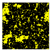
(a) Replica 1.

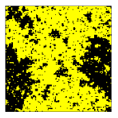
(b) Replica 2.

(c) Soft-constraint clusters.

(d) Hard-constraint clusters.

Figure 1: Spin configurations as well as soft- and hard-constraint geometrical clusters of the two-dimensional Ising model at the Ising critical temperature $T_{\text{c}}$. (1(a)) Spin configuration of the first replica. (1(b)) Spin configuration of the second replica. (1(c)) The resulting soft-constraint clusters. (1(d)) The resulting hard-constraint clusters. In (1(c)) and (1(d)) all clusters, apart from the largest percolating one, are assigned colours at random. For the largest percolating cluster of both the soft- and hard-constraint definitions, the same colour (black) is assigned.

In overlap space we may then define geometrical clusters, i.e., sets of neighboring lattice sites with the same values of the overlap, that can be formed in two particular ways:

1. Soft-constraint clusters are created by joining spins on neighboring sites $(i,j)$ with $q_{i}=q_{j}$.

2. Hard-constraint clusters are formed by joining neighboring spins with $s_{i}^{(1)}=s_{j}^{(1)}$ and $s_{i}^{(2)}=s_{j}^{(2)}$.

From the above it is obvious that the hard-constraint clusters trivially satisfy $q_{i}=q_{j}$ and they are a subset of the soft-constraint clusters. The construction of these clusters is illustrated through the snapshots shown in Fig. 1, where configurations of the two replicas are shown (top row) along with the soft- and hard-constraint clusters (bottom row) for a system of linear size $L=128$ at the critical temperature of the square-lattice Ising model. It is apparent that the typical clusters in the overlap are smaller than those in the two replicas, and that the hard constraint leads to smaller clusters than the soft constraint. We note that in the spin-glass setup, the prescription for soft-constrained clusters leads to what is there known as Houdayer clusters [28], while the hard constraint corresponds to a geometric-cluster version of the Chayes-Machta-Redner construction [32, 30].

In the present work, we studied these clusters for the case of the Ising model on the square lattice. In particular, we simulated the Ising model by considering two replicas on the square lattice with periodic boundary conditions for a range of temperatures including the exact Ising critical temperature, i.e., $T_{\text{c}}=2/\left(1+\sqrt{2}\right)\approx 2.269185$. Configurations were generated via the Swendsen-Wang algorithm [13] applied to systems of linear sizes in the range $8\leq L\leq 2048$. For all system sizes and on each replica the total number of simulation steps was $1.1\times\tau_{\text{int, E}}\times 10^{5}$ sweeps, of which $\tau_{\text{int, E}}\times 10^{4}$ sweeps were discarded during equilibration. Here, $\tau_{\text{int, E}}$ denotes the integrated autocorrelation time of the energy [33]. After every $\tau_{\text{int, E}}$ sweeps a measurement was taken, resulting in $10^{5}$ measurements per run. The estimates of $\tau_{\text{int, E}}$, rounded up to the next largest integer, varied from $5$ sweeps for $L=8$ to $15$ sweeps for $L=2048$. Note that in order to identify wrapping clusters we employed the method of Machta et al. [34]. Finally, for all curve fitting performed throughout this paper we restricted ourselves to data with $L\geq L_{\rm min}$, adopting the standard $\chi^{2}$ test for goodness of the fit. Specifically, we considered a fit as being acceptable only if $Q>0.01$, where $Q$ is the quality-of-fit parameter [35].

III Observables

To investigate the percolation transition of geometrical overlap clusters, the main relevant quantities are the percolation strength $P_{\infty}$, the average cluster size $S$, and the wrapping probability $R$ [10]. The latter is defined as the probability that, given a spin configuration, at least one cluster wraps around the periodic boundaries of a finite lattice and is connected back to itself. In the thermodynamic limit, one expects that $R=1$ for temperatures below the percolation transition at $T_{p}$, and $R=0$ at temperatures above $T_{p}$. The wrapping of a cluster can occur in various ways, and here we consider the following cases, in analogy to Ref. [36]:

1. $R_{\text{x or y}}$ is the probability that a cluster wraps around the lattice in horizontal or vertical (or both) direction(s).

2. $R_{\text{x and y}}$ is the probability that a cluster wraps in horizontal and in vertical direction.

3. $R_{\text{x}}$ is the probability that a cluster wraps in horizontal direction. Obviously, on the square lattice the probability that a cluster wraps in vertical direction $R_{\text{y}}\equiv R_{\text{x}}$.

4. $R_{\text{x and }\overline{\text{y}}}$ is the probability that a cluster wraps around one but not the other direction. Here we choose the probability that a cluster wraps around the horizontal and not the vertical direction. The symmetry of the square lattice indicates that $R_{\text{x and }\overline{\text{y}}}\equiv R_{\text{y and }\overline{\text{x}}}$.

The wrapping probability $R$ is a dimensionless quantity, and so one expects finite-size scaling of the form [10, 37]

$$R=\tilde{R}\left[\left(T-T_{\text{p}}\right)L^{1/\nu}\right].$$ (3)

Hence, the $R$ curves for systems of different sizes are expected to cross, up to finite-size corrections, at the same point, marking the transition temperature $T_{\mathrm{p}}$. In addition, since the scaling function $\tilde{R}$ is expected to be universal, so is the value of $R=\tilde{R}(0)$ at the crossing point [10]. This behavior is nicely verified in Figs. 2 and 3, where the various wrapping probabilities are plotted as a function of temperature $T$ for the larger system sizes studied and for both soft- and hard-constraint clusters. Except for $R_{\text{x and }\overline{\text{y}}}$, all wrapping probabilities increase with decreasing temperature, indicative of the onset of the percolating phase. The crossing of data sets for different system sizes is found to occur very close to the critical temperature $T_{\mathrm{c}}$ of the Ising model shown in Figs. 2 and 3 as a dashed vertical line. This latter observation also holds for $R_{\text{x and }\overline{\text{y}}}$ with the essential difference that this observable exhibits a maximum, the position of which is expected to shift to its asymptotic value as $L\rightarrow\infty$ [36]. In numerical studies of ordinary percolation, however, it was shown that $R_{\text{x and }\overline{\text{y}}}$ exhibits both crossing points and maxima only in three dimensions [38], whereas in two dimensions the crossing region is absent [36, 38]. Thus, the existence of both maxima and crossing points in $R_{\text{x and }\overline{\text{y}}}$ in two dimensions marks an interesting feature of the percolation signature of geometrical clusters in the overlap of the Ising model.

Figure 2: Wrapping probabilities $R^{\text{(s)}}$ of the soft-constraint clusters as a function of temperature $T$ for (a) $R_{\text{x or y}}^{\text{(s)}}$, (b) $R_{\text{x and y}}^{\text{(s)}}$, (c) $R_{\text{x}}^{\text{(s)}}$, and (d) $R_{\text{x and }\overline{\text{y}}}^{\text{(s)}}$. Only results for the larger system sizes are shown ($L\geq 320$). Here and in the following, the dashed vertical lines mark the critical temperature $T_{\mathrm{c}}$ of the Ising model.

Figure 3: Wrapping probabilities $R^{\text{(h)}}$ of the hard-constraint clusters as a function of temperature $T$, analogous to the data for soft-constraint clusters shown in Fig. 2.

Of central importance in percolation theory is the cluster number $n_{s}$, denoting the expected number of clusters of $s$ sites per lattice site [10]. Thus the average cluster size can be expressed as

$$S=\frac{\sum_{s^{\prime}}s^{2}n_{s}}{\sum_{s^{\prime}}sn_{s}},$$ (4)

where $sn_{s}$ corresponds to the probability of a randomly picked site to belong to a cluster of size $s$. The notation $s^{\prime}$ indicates that the sums are restricted to certain subsets of clusters. Denoting the set of clusters in a configuration as $C$ and letting $P$ be a subset of $C$ containing the percolating clusters, we can introduce the following definitions for $S$:

1. All clusters are included: $C$.

2. Exclude the largest cluster in each measurement: $C\;\backslash\;\text{max}\;C$.

3. Exclude all percolating clusters: $C\;\backslash\;P$.

4. Exclude all clusters percolating in horizontal and in vertical direction: $C\;\backslash\;P_{\text{x and y}}$.

5. Exclude all clusters percolating in one specific direction, e.g., horizontal: $C\;\backslash\;P_{\text{x}}$.

6. Exclude all clusters percolating in one but not the other direction, e.g., horizontal and not vertical: $C\;\backslash\;P_{\text{x and }\overline{\text{y}}}$.

Figure 4: Average cluster size $S$ according to the definition $C\;\backslash\;\text{max}\;C$ as a function of temperature on a semi-logarithmic scale. Results for both (a) soft-constraint and (b) hard-constraint clusters are presented for the larger system sizes studied ($L\geq 320$).

In most numerical studies of percolation the employed definition of the average cluster size excludes the largest cluster in each measurement, corresponding to our case (2) [10]. With this convention, $S$ has a maximum around the percolation point, since in the non-percolating phase the size of many contributing clusters increases, while in the percolating regime most spins belong to the largest cluster which is not counted towards the sum. This estimate is shown in Fig. 4 where $S$ is plotted as a function of $T$ for the larger system sizes and for both soft- and hard-constraint clusters. In the vicinity of the percolation point, the average cluster size is expected to follow a scaling form according to [10]

$$S\left(L,T\right)=L^{\gamma/\nu}\tilde{S}\left[\left(T-T_{\text{p}}\right)L^{1/\nu}\right],$$ (5)

which can be used for determining the critical exponent ratio $\gamma/\nu$ conventionally associated to the scaling of the magnetic susceptibility.

The percolation strength $P_{\infty}$ corresponds to the fraction of sites belonging to the infinite cluster in the thermodynamic limit. For finite-size systems it is usually estimated from the fraction of sites belonging to the largest cluster. In Fig. 5, $P_{\infty}$ is plotted against $T$ for the full range of system sizes studied and for both soft- and hard-constraint clusters. Note that (i) as the temperature decreases $P_{\infty}$ increases, indicating the appearance of a percolating cluster, and (ii) for $T=0$ we have $P_{\infty}=1$ as all spins belong to the percolating cluster. We remind that when studying the FK clusters in magnetic systems, the percolation strength corresponds to the magnetization of the system [11]. Finite-size scaling theory suggests a scaling form

$$P_{\infty}\left(L,T\right)=L^{-\beta/\nu}\tilde{P}_{\infty}\left[\left(T-T_{\text{p}}\right)L^{1/\nu}\right],$$ (6)

where $\beta/\nu$ denotes the corresponding critical exponent ratio.

Figure 5: Percolation strength $P_{\infty}$ as a function of temperature for both (a) soft-constraint and (b) hard-constraint clusters. For clarity, only the legends of the smallest and largest system sizes are highlighted.

Analogous to the treatment of $R$ and $S$, it is natural to also consider modified percolation strengths $P_{\infty}$ by studying the fractions of sites occupied by the following subsets:

1. Largest cluster: $\text{max}\;C$.

2. Largest percolating cluster: $\text{max}\;P$.

3. Largest cluster that percolates in horizontal and in vertical direction: $\text{max}\;P_{\text{x and y}}$.

4. Largest cluster that percolates in one specific direction, e.g., horizontal: $\text{max}\;P_{\text{x}}$.

5. Largest cluster that percolates in one but not the other direction, e.g., horizontal and not vertical: $\text{max}\;P_{\text{x and }\overline{\text{y}}}$.

In the following, we will use the scaling forms (3), (5) and (6) with the universal scaling functions $\tilde{R}$, $\tilde{P}_{\infty}$, and $\tilde{S}$ in order to determine the correlation-length critical exponent $\nu$ as well as the exponent ratios $\gamma/\nu$ and $\beta/\nu$ of the average cluster size and the percolation strength, respectively, as well as the percolation temperature $T_{\mathrm{p}}$.

Figure 6: Maximum slope of the wrapping probability, $\left|\mathrm{d}R/\mathrm{d}T\right|_{\text{max}}$, as a function of system size $L$ on a double logarithmic scale for all variants of the wrapping probabilities and for (a) soft-constraint and (b) hard-constraint clusters.

IV Main Results

IV.1 Correlation-length exponent

In Monte Carlo studies of phase transitions the temperature-derivative of the Binder cumulant [39] provides a reliable estimate for the critical exponent $\nu$ [40]. In random percolation, a similar behavior is expected for the derivative of the wrapping probability with respect to the bond occupation probability [38]. For the present problem of clusters in a thermal problem it is natural, in contrast, to consider the temperature-derivative of the wrapping probabilities. As the latter are monotonic functions of the temperature — except for $R_{\text{x and }\overline{\text{y}}}$ — one expects that the maximum of the absolute value of its first derivative should scale as

$$\left|\frac{\mathrm{d}R}{\mathrm{d}T}\right|_{\text{max}}\sim L^{1/\nu}.$$ (7)

As shown in Sec. III, the exception to this rule is $R_{\text{x and }\overline{\text{y}}}$ which is a non-monotonic function of $T$, showing both a maximum and a crossing region. Nevertheless, if we restrict ourselves to the vicinity of the crossing regime, this observable is also expected to follow the scaling behaviour of Eq. (7). Importantly, Eq. (7) allows one to obtain estimates of $\nu$ without prior knowledge of the percolation temperature $T_{\mathrm{p}}$. To determine the maximum of $\left|\mathrm{d}R/\mathrm{d}T\right|$, both the first and second derivatives are computed using the symmetric-finite-difference definition, and the root is located using the bisection method [35]. The required estimates at nearby temperatures are extracted from the simulation data by means of single-histogram reweighting [41], using a step size $\Delta T=10^{-7}$.

In Fig. 6, $\left|\mathrm{d}R/\mathrm{d}T\right|_{\text{max}}$ is shown as a function of $L$ for the different wrapping probabilities of the soft- and hard-constraint clusters. Fits of the form (7) were performed for system sizes on intervals $L_{\text{min}}\leq L\leq L_{\text{max}}$ by systematically increasing the lower cut-off $L_{\text{min}}$, while keeping the upper cut-off fixed at $L_{\text{max}}=2048$. The resulting effective values of $\nu$ are shown in Fig. 7. The final estimates we quote for both the soft- and hard-constraint clusters using the $R_{\text{x and y}}^{(\text{s})}$ and $R_{\text{x and }\overline{\text{y}}}^{(\text{h})}$ definitions, respectively, are

$$\nu^{\text{(s)}}=1.005(5)\;\;(L_{\text{min}}=256),\\$$ (8a)

$$\nu^{\text{(h)}}=1.00(3)\;\;(L_{\text{min}}=800).$$ (8b)

These results suggest that the critical exponent of the correlation length is the same for both cluster types and consistent with that of the Ising model, i.e., $\nu=1$.

Figure 7: Effective values of the exponent $\nu$ vs. the inverse lower cutoff size $1/L_{\text{min}}$ on a semi-logarithmic scale. The estimates were obtained from fits of the form (7) to the data of Fig. 6.

IV.2 Percolation temperature

For the estimation of the percolation temperature $T_{\text{p}}$ we considered the intersection of the wrapping probabilities of pairs of system sizes $(L,L^{\prime})$ as a function of $T$, following the original prescription by Binder for the magnetization cumulant [39, 40]. The points where these wrapping probabilities cross scale as [39]

$$T_{\text{cross}}\left(L,b\right)=T_{\text{p}}+aL^{-\left(1/\nu+\omega\right)}\left(\frac{b^{-\omega}-1}{b^{1/\nu}-1}\right),$$ (9)

where $a$ is a non-universal scaling parameter, $\omega$ is the corrections-to-scaling exponent, and $b=L^{\prime}/L$ is the quotients ratio, fixed hereafter to $b=2$. Crossings were determined using the bisection method [35] alongside the single-histogram reweighting technique [41].

Figure 8: Estimates of crossing temperatures for (a) soft-constraint and (b) hard-constraint clusters on a semi-logarithmic scale. The dashed horizontal line marks the transition temperature of the Ising model.

Figure 8 showcases the scaling of the crossing points of the various wrapping probabilities for both the soft- and hard-constrained clusters, which appear to be consistent with the critical temperature of the Ising model, up to surprisingly small finite-size effects. In order to obtain more accurate estimates of $T_{\text{p}}$ we performed fits using Eq. (9). Due to the smallness of the corrections, however, the accuracy of our data did not allow us to resolve their detailed form, resulting in fits of poor quality and consequently in unreliable estimates of the involved parameters. As an alternative, we fixed $\nu$ to the expected value $\nu=1$, so that Eq. (9) (ignoring scaling corrections) simplifies to

$$T_{\text{cross}}=T_{\text{p}}+a/L.$$ (10)

Figure 9: Estimates of the percolation temperature $T_{\mathrm{p}}$ vs. $1/L_{\rm min}$ on a semi-logarithmic scale. Results obtained from fits of the form (10) on the data of Fig. 8. The dashed horizontal line marks here as well the transition temperature of the Ising model.

Estimates of the percolation temperature resulting from the linear fits of Eq. (10) are shown in Fig. 9 for both soft- and hard-constraint clusters; they are found to be consistent with the critical temperature of the Ising ferromagnet, i.e., $T_{\rm c}=2.269185\ldots$. We note that the results for $R_{\text{x or y}}$ have slightly elevated statistical errors as compared to the other definitions, a feature that can be traced back to the fact that $R_{\text{x or y}}$ is very close to one at $T_{c}$ such that the curves cross at a smaller angle, cf. Figs. 2(a) and 3(a). In addition, the parameter $a$ of Eq. 10 for all fits is consistent with zero within error bars, indicating that the data can also be described by a constant $T_{\mathrm{cross}}(L)=T_{\mathrm{p}}=T_{\mathrm{c}}$, independent of $L$. At this point we may safely conclude that soft- and hard-constraint clusters undergo a percolation transition at the critical temperature $T_{\mathrm{c}}$ of the Ising model.

IV.3 Scaling at criticality

We proceed with the computation of critical exponents related to the percolation strength, $P_{\infty}$, and the average cluster size, $S$, for the two types of clusters at criticality. Since we found convincing evidence of the identity of the percolation and critical exponents, $T_{\mathrm{p}}=T_{\mathrm{c}}=2.269185\ldots$ in the previous section, we considered the scaling of $P_{\infty}$ and $S$ at the fixed temperature $T=T_{\mathrm{c}}$; the result is shown for the soft- and hard-constraint clusters in Figs. 10 and 11, respectively. For both observables, all data appear to follow straight parallel lines, suggesting minor corrections to scaling and universal exponents, independent of the definition used.

Figure 10: Percolation strength $P_{\infty}$ vs. $L$ at the critical temperature of the Ising model on a double logarithmic scale for (a) soft-constraint and (b) hard-constraint clusters.

Figure 11: Average cluster size $S$ vs. $L$ at the critical temperature of the Ising model on a double logarithmic scale for (a) soft-constraint and (b) hard-constraint clusters.

At the percolation point, according to Eqs. (5) and (6) the scaling functions become constant, thus allowing for the estimation of the involved exponents from finite-size scaling. In the following, we present the results of systematically fitting those functional forms to the data for $P_{\infty}$ and $S$ for all sets of definitions, following the established protocol of varying $L_{\rm min}$ as described above, allowing us to monitor the influence of corrections to scaling.

Figure 12 shows our estimates of the effective exponent ratios $\left(\beta/\nu\right)^{\text{(s)}}$ and $\left(\beta/\nu\right)^{\text{(h)}}$ while varying the cutoff $L_{\rm min}$. Besides the $\text{max}\;P_{\text{x and }\overline{\text{y}}}$ data, it is evident that the exponents converge relatively quickly to the values $\left(\beta/\nu\right)^{\text{(s)}}\approx 0.095$ and $\left(\beta/\nu\right)^{\text{(h)}}\approx 0.12$ for the soft- and hard-constraint clusters, respectively. The fact that the numerical data for the $\text{max}\;P_{\text{x and }\overline{\text{y}}}$ definition provide unreliable estimates of the involved exponent can be readily understood: clusters percolating in one but not the other direction are sparse, leading to poor statistics in the estimation of the percolation strength and the associated exponent. This observation has also been reported in Ref. [42] for the Ising model.

As there is no systematic trend visible in our data that could possible reveal the existence of corrections to scaling for $\left(\beta/\nu\right)^{\text{(s)}}$ and $\left(\beta/\nu\right)^{\text{(h)}}$, we did not attempt to perform fits including correction terms. Instead, as a trade-off between unavoidable corrections to scaling and reasonable values of $\chi^{2}$, we choose sufficiently large $L_{\mathrm{min}}$ for our final estimates of $\left(\beta/\nu\right)^{\text{(s)}}$ and $\left(\beta/\nu\right)^{\text{(h)}}$,

$$\left(\frac{\beta}{\nu}\right)^{\text{(s)}}=0.0950(7)\;\;(L_{\text{min}}=320),\\$$ (11a)

$$\left(\frac{\beta}{\nu}\right)^{\text{(h)}}=0.1184(11)\;\;(L_{\text{min}}=512).$$ (11b)

Figure 12: Effective exponent ratios $\beta/\nu$ extracted from fits of the functional forms (5) and (6) as a function of the inverse lower size cut-off $1/L_{\text{min}}$ for (a) soft-constraint and (b) hard-constraint clusters.

Estimates for the effective exponent ratios $\left(\gamma/\nu\right)^{\text{(s)}}$ and $\left(\gamma/\nu\right)^{\text{(h)}}$ are shown in Fig. 13. For the $C$ and $C\;\backslash\;P_{\text{x and }\overline{\text{y}}}$ definitions, the exponent ratio converges relatively quickly to the value $\left(\gamma/\nu\right)^{\text{(s)}}\approx 1.81$ and $\left(\gamma/\nu\right)^{\text{(h)}}\approx 1.77$ for the soft- and hard-constraint clusters respectively, indicating that corrections to scaling are not substantial. On the other hand, for the rest of the definitions, corrections to scaling become important and the convergence to an asymptotic value is rather slow. The fact that $C$ and $C\;\backslash\;P_{\text{x and }\overline{\text{y}}}$ give similar results is to be expected, as the latter definition excludes clusters that rarely appear, thus not altering significantly the sums in Eq. (4). Note that the reduction of scaling corrections for the average cluster size through the choice of the $C$ definition was also reported in Ref. [24] for the Ising model, while a systematic study of the behavior for the Ising model from all of the above definitions was presented in Ref. [42].

Figure 13: Effective exponent ratios $\gamma/\nu$ vs. $1/L_{\text{min}}$ for (a) soft-constraint and (b) hard-constraint clusters.

More reliable estimates for the exponent ratio $\gamma/\nu$ can be retrieved by taking into account corrections to scaling for both soft- and hard-constraint clusters. To arrive at somewhat stable estimates for the correction-to-scaling exponent, we performed joint fits to the data for the different definitions of $S$ including one correction term using the Ansatz

$$S=aL^{\gamma/\nu}\left(1+bL^{-\omega}\right),$$ (12)

where $a$ and $b$ are the non-common fitting parameters and $\gamma/\nu$, and $\omega$ the shared parameters. Since data from different definitions are not statistically independent, as they result from the same Monte Carlo series, a naive implementation of the above fitting procedure will result in erroneous error estimation of the fit parameters. Thus, in order to provide reliable estimates for the errors of the involved parameters, we employed the jackknife method [43]. For all values of $L_{\text{min}}$, estimates of $\gamma/\nu$ agree within error bars as is shown in Fig. 14. Additionally, in Fig. 15 the exponent $\omega$ is plotted as a function of $L_{\text{min}}$. The fact that the error bars in the estimates of $\gamma/\nu$ and $\omega$ are increasing with $L_{\text{min}}$ is of course a consequence of the decreasing number of degrees of freedom. However, the errors in $\omega$ increase rapidly, and for $L_{\text{min}}\geq 320$ they are comparable with their absolute values for both cluster types. Our final estimates of the involved exponent ratio $\gamma/\nu$ of the soft- and hard-constraint clusters are:

$$\left(\frac{\gamma}{\nu}\right)^{\text{(s)}}=1.814(5)\;\;(L_{\text{min}}=200),\\$$ (13a)

$$\left(\frac{\gamma}{\nu}\right)^{\text{(h)}}=1.765(4)\;\;(L_{\text{min}}=200).$$ (13b)

We note that the estimated value of $\omega\approx 0.2$ for both soft- and hard-constraint clusters represents a rather slow decay of corrections, consistent with the slow convergence of $\gamma/\nu$ for most definitions of $S$ that is clearly visible in Fig. 13. We are not aware of any theoretical estimates relating to the value of $\omega$.

Figure 14: Exponent ratio $\gamma/\nu$ resulting from the joint fit of all definitions as a function of $1/L_{\text{min}}$ for (a) soft-constraint and (b) hard-constraint clusters.

Figure 15: Corrections-to-scaling exponent $\omega$ resulting from the joint fit of all definitions as a function of $1/L_{\text{min}}$ for (a) soft-constraint and (b) hard-constraint clusters.

IV.4 Fractal dimension and hyperscaling

At the percolation point the incipient spanning cluster is a fractal object and its mass $M$ (i.e., the number of spins that belong to the spanning cluster) scales with the system size as $M\sim L^{D}$. Here, $D$ denotes the fractal dimension of the incipient spanning cluster. Since from the discussion in Sec. III the percolation strength $P_{\infty}$ corresponds to the fraction of spins in the percolating cluster, it follows that $D=d-\beta/\nu$. From the estimates of $\beta/\nu$ for the soft- and hard-constraint clusters provided in Eqs. (11a) and (11b) we hence obtain

$$D^{\text{(s)}}=1.9050(7);\;\;D^{\text{(h)}}=1.8816(11),$$ (14)

suggesting that the fractal dimension is different for the two cluster types. Also, the fact that $D^{\text{(s)}}>D^{\text{(h)}}$ highlights that the soft-constraint clusters are denser than the hard-constraint ones, a reasonable expectation as the hard-constraint clusters are a subset of the soft-constraint ones. Additionally, let us point out that the fractal dimensions for both cluster types are smaller than $D=187/96\approx 1.9479$, the fractal dimension of geometrical clusters in the Ising model [20].

On the other hand, if hyperscaling is valid, the fractal dimension can also be estimated from $D=\beta/\nu+\gamma/\nu$ [10]. Combining our estimates from Eqs. (11a) and (11b) with (13a) and (13b), we arrive at

$$D^{\text{(s)}}=1.909(5);\;\;D^{\text{(h)}}=1.883(4),$$ (15)

which is consistent with the estimates of Eq. (14), thus illustrating that hyperscaling is valid for both cluster types.

V Discussion

We have studied the percolation properties of clusters defined in the overlap space of two statistically independent systems of the square-lattice Ising model. To this end, two distinct cluster types were introduced which we dubbed soft- and hard-constraint clusters. After a short exposition of the behavior of the main observables, i.e., the wrapping probabilities, average cluster sizes, and percolation strengths, the critical behavior of the system was investigated. Our results indicate that both cluster types are described by the same correlation length exponent which is found to be in agreement with the value $\nu=1$ of the Ising ferromagnet. Additionally, both cluster types percolate at a temperature that is indistinguishable from the transition point of the two-dimensional Ising model for the lattice sizes up to $L=2048$ that we considered in our study. In marked contrast with the exponent $\nu$, our analysis for the exponent ratios $\beta/\nu$ and $\gamma/\nu$ manifests the following: (i) the exponent values are clearly different from those that characterize the geometrical clusters of the Ising model, and (ii) there is a small but seemingly systematic difference in the exponents estimated for the soft-constraint and the hard-constraint clusters, cf. the overview of exponent estimates provided in Table 1.

Table 1: Critical exponents of the soft- and hard-constraint clusters in comparison to the exact values of the geometrical clusters of the square-latice Ising model model.

	overlap		Ising
	soft	hard	$-$
$\nu$	1.005(5)	1.00(3)	1
$\beta/\nu$	0.0950(7)	0.1184(11)	$5/96\approx 0.052$
$\gamma/\nu$	1.814(5)	1.765(4)	$91/48\approx 1.895$
$D=\gamma/\nu+\beta/\nu$	1.909(5)	1.883(4)	$187/96\approx 1.947$
$D=d-\beta/\nu$	1.9050(7)	1.8816(11)	$187/96$

Under the assumption that $T_{\mathrm{p}}=T_{\mathrm{c}}$ that is so well corroborated by our numerical results, the scaling exponents for the overlap clusters can be deduced from the following argument: according to the expected scaling of $P_{\infty}$, at $T_{\mathrm{c}}$ the probability of a randomly picked site to be in the percolating cluster of replica one scales as $\sim L^{-(\beta/\nu)_{\mathrm{IG}}}$, where $(\beta/\nu)_{\mathrm{IG}}=5/96$ corresponds to the exponent of the geometrical clusters in the Ising model. As the same holds for replica two and the two replicas are uncorrelated, the probability of the site being in the percolating cluster of both replicas decays as $\sim L^{-2(\beta/\nu)_{\mathrm{IG}}}$, such that $\beta/\nu=2(\beta/\nu)_{\mathrm{IG}}=10/96\approx 0.1042$. As a consequence, one expects $\gamma/\nu=2-4(\beta/\nu)_{\mathrm{IG}}=43/24\approx 1.792$ and $D=2-2(\beta/\nu)_{\mathrm{IG}}=91/48\approx 1.8958$. As a glance at Table 1 shows, these values are quite compatible with our findings in particular for the hard-constraint clusters to which this type of argument applies. The small deviations observed might be a consequence of the slow decay of scaling corrections expressed in the small value $\omega\approx 0.2$ of the Wegner exponent. The clusters in the soft-constraint problem are, by construction, larger than those of the hard-constraint variant, but their scaling does not directly follow from the above argument, so it is possible that they show asymptotically different exponents.

At the same time, the density of the percolating cluster in the overlap is below that of the percolating spin cluster in a single Ising model, while the clusters of the former are also found to be more compact than those in the latter. This is a natural consequence of the superimposition of the two fractal structures such that the objects investigated here correspond to their intersection. It would be most intriguing to study how clusters in the mutual overlap of more than two copies of the system behave — a task which is left for future work, however.