A Robust Twin Parametric Margin Support Vector Machine for Multiclass Classification

Abstract

In this paper we present a Twin Parametric-Margin Support Vector Machine (TPMSVM) model to tackle the problem of multiclass classification. In the spirit of one-versus-all paradigm, for each class we construct a classifier by solving a TPMSVM-type model. Once all classifiers have been determined, they are combined into an aggregate decision function. We consider the cases of both linear and nonlinear kernel-induced classifiers. In addition, we robustify the proposed approach through robust optimization techniques. Indeed, in real-world applications observations are subject to measurement errors and noise, affecting the quality of the solutions. Consequently, data uncertainties need to be included within the model in order to prevent low accuracies in the classification process. Preliminary computational experiments on real-world datasets show the good performance of the proposed approach.

1 Literature review

Support Vector Machine (SVM) is introduced in Vapnik (1982) with the aim of solving a binary classification problem with two linearly separable classes. The generalization of the linear approach is proposed in Boser et al. (1992) by including nonlinear decision boundaries induced by kernel functions (see Schölkopf and Smola (2001). In order to deal with not perfectly separable input data, in Vapnik (1995) a vector $\xi$ of slack variables is introduced. The resulting model seeks for a trade-off between the maximization of the margin, as in the classical SVM approach of Vapnik (1982), and a minimization of the magnitude of $\xi$. This is performed with both linear and nonlinear classifiers.
To increase the predictive power of the SVM, several alternative formulations have been proposed in the literature. In Schölkopf et al. (2000) a new class of SVM-type algorithms is designed. This paradigm is called $\nu$-Support Vector Classification since it involves a positive parameter $\nu$ in the objective function, bounding the fractions of supporting vectors and errors. Basing on this approach, in Hao (2010) a parametric-margin model (the par-$\nu$-SVM) is introduced to deal with the case of heteroscedastic noise, is introduced. Contrariwise to the original approach, in Liu and Potra (2009) two parallel hyperplanes are constructed, one for each class. The optimal classifier is then searched in the region between the hyperplanes and is such that the total number of misclassified points is minimized. The generalization with nonlinear classifiers has been recently proposed in Maggioni and Spinelli (2023). Instead of dealing with parallel hyperplanes to classify input observations, in Jayadeva et al. (2007) the Twin Support Vector Machine (TWSVM) considers two nonparallel hyperplanes by solving two smaller sized SVM-problems. Consequently, the computational complexity of TWSVM is approximately one-fourth of the original SVM. Due to its favourable performances, especially when handling large datasets (see Tanveer et al. (2022)), many variants of the TWSVM approach have been proposed in the literature: Least Squares TWSVM (LS-TWSVM, Arun Kumar and Gopal (2009)), Projection TWSVM (P-TWSVM, Chen et al. (2011)), Pinball loss TWSVM (Pin-TWSVM, Xu et al. (2017)), Twin Parametric-Margin SVM (TPMSVM, Peng (2011)). For a comprehensive review on recent developments on TWSVM the reader is referred to Tanveer et al. (2022).
Among all the possible variants of TWSVM, in this paper we focus our attention on the TPMSVM. This choice is motivated by its generalization ability, good training time and suitability when input data are subject to noise (Tanveer et al. (2022)). This formulation combines the ideas of TWSVM and par-$\nu$-SVM. Specifically, it aims at generating two nonparallel hyperplanes (or kernel-induced decision boundaries in the nonlinear context), each of them determining the positive or negative parametric-margin of the separating classifier (see Peng (2011)). In addition, it integrates the fast learning speed of the TWSVM and the flexible parametric-margin of the par-$\nu$-SVM.
All the approaches discussed so far consider the case of a binary classification. However, in real-world applications the classifying categories might be more than two. In the literature there exist two groups of approaches to tackle the problem of multiclass classification: all-together methods and decomposition-reconstruction methods (Ding et al. (2019)). In the first approach all data are considered in one large optimization model and the classifier is derived accordingly (see Bredensteiner and Bennett (1999), Yajima (2005), Zhong and Fukushima (2007)). On the other hand, within the decomposition-reconstruction methods, the multiclass classification problem is decomposed into a sequence of binary classification problems. Each of them is solved independently and the binary classifiers are then combined into a multiclass decision function. The decomposition-reconstruction procedure is considered to be the most effective way to achieve multiclass separation (Du et al. (2021)), especially due to the high complexity of the all-together methods with large datasets (Ding et al. (2019)). Within the decomposition-reconstruction paradigm, different formulations have been designed. In the one-versus-all strategy (Xie et al. (2013)) one classifier for each class is generated. Specifically, when focusing on the $c$-th class, for $c=1,\ldots,C$ with $C$ the total number of classes, a binary classifier separating “class $c$” and “non-class $c$” points is determined by solving a SVM-type model. In the one-versus-one strategy (Hastie and Tibshirani (1998)) $C(C-1)/2$ binary classifiers are built, one for each pair of classes. Consequently, only the samples of the selected classes are considered in the optimization model. In contrast, in the one-versus-one-versus-rest framework (Angulo et al. (2003)) all observations are utilized in constructing the classification rule. Indeed, each subproblem focuses on the separation of a pair of classes together with all the remaining data by means of two hyperplanes. Each hyperplane is close to a class and as far as possible from the other, with all the remaining points restricted in a region between the two hyperplanes (Du et al. (2021)). Other decomposition-reconstruction approaches are direct acyclic graph (Platt et al. (1999)), all-versus-one (Yang et al. (2013)) and binary tree SVM structure (Shao et al. (2013)). A review on multiclass models especially designed for TWSVM can be found in Ding et al. (2019).
For the methods mentioned above, all data points are implicitly assumed to be known exactly. Unfortunately, training observations may be subject to perturbations due to measurement errors in the data collection process. Robust Optimization (RO) (see Xu et al. (2009)) is one of the most explored approaches to handle problems affected with uncertainty. A robust formulation of the linear SVM in Cortes and Vapnik (1995) is provided in Bertsimas et al. (2019). Similarly, the robust counterparts of the linear and nonlinear approach of Liu and Potra (2009) are derived in Faccini et al. (2022) and in Maggioni and Spinelli (2023), respectively. As far as it concerns RO techniques applied in the context of TWSVM, in Peng and Xu (2013) a robust minimum class variance model is proposed. Specifically, a pair of uncertain class variance matrices is included in the objective function and uncertainty set around the true covariance matrix of each class is constructed according to the Frobenius norm. In the spirit of TWSVM, in Qi et al. (2013) two nonparallel classifiers are proposed to derive the final decision function in the case of ellipsoidal uncertainty set. The corresponding model is then reformulated as a Second Order Cone Programming (SOCP). In the case of kernel-induced classifiers, only the case with Gaussian kernel is explored. Instead of convex hulls to represent the training patterns, López et al. (2019) consider ellipsoids given by the first two moments of the class distributions. The robust problem is formulated as a chance-constrained programming model (Shapiro et al. (2009)) and the robust counterpart reduces to a SOCP formulation. Within the multiclass framework, in Zhong and Fukushima (2007) a robust classification through piecewise-linear functions is derived, robustifying the approach of Bredensteiner and Bennett (1999).
In this paper, we present a novel TPMSVM-type model for multiclass classification. We consider both the cases of linear and kernel-induced decision boundaries. Given the uncertain nature of real-world observations, we derive robust counterparts of the nominal models by considering a general bounded-by-$\ell_{p}$-norm uncertainty set around each input data. We test the proposed methodology on publicly available datasets to assess their accuracy.
The remainder of the paper is organized as follows. Section 2 introduces notation and basic facts on binary TPMSVM model. In Section 3 the deterministic multiclass models are designed, while in Section 4 their robust counterparts are presented. Section 5 reports preliminary computational results to evaluate the accuracy of the proposed formulations. Finally, in Section 6 conclusions and future works are provided.

2 Background

In this section, we report the notation and we recall the main characteristics of the binary TPMSVM model.

2.1 Notation

In this paper, all vectors are column vectors, unless transposed to row vectors by the superscript “^⊤”. For $p\in[1,\infty]$ and $a\in\mathbb{R}^{n}$, $\left\lVert a\right\rVert_{p}$ is the $\ell_{p}$-norm of $a$. The dot product in a inner product space $\mathcal{H}$ will be denoted by $\langle\cdot,\cdot\rangle$. If $\mathcal{H}=\mathbb{R}^{n}$ and $a,b\in\mathbb{R}^{n}$, $a^{\top}b$ is equivalent to $\langle a,b\rangle$. If $\mathcal{A}$ is a set, $\left\lvert\mathcal{A}\right\rvert$ represents its cardinality. In addition, we denote by $e$ a column vector of ones of arbitrary dimension.

2.2 The linear TPMSVM

Let $\{x^{i},y_{i}\}_{i=1}^{m}$ be the set of training observations, where $x^{i}\in\mathbb{R}^{n}$ is the vector of features, and $y_{i}\in\{-1,+1\}$ is the label of the $i$-th data point, representing the negative or positive class to which it belongs. We assume that each of the two classes is composed by $m_{-}$ and $m_{+}$ observations, respectively, with $m_{-}+m_{+}=m$. We denote by $X_{-}\in\mathbb{R}^{n\times m_{-}}$ and $X_{+}\in\mathbb{R}^{n\times m_{+}}$ the matrices of the negative and positive data points, respectively, whereas $\mathcal{X}_{-}$ and $\mathcal{X}_{+}$ correspond to the indices sets.
The TPMSVM (see Peng (2011)) finds two nonparallel parametric-margin hyperplanes $H_{+}$ and $H_{-}$, defined by the following equations:

$$H_{+}:w_{+}^{\top}x+\theta_{+}=0\qquad H_{-}:w_{-}^{\top}x+\theta_{-}=0,$$ (1)

where $w_{+},w_{-}\in\mathbb{R}^{n}$ are the normal vectors and $\theta_{+},\theta_{-}\in\mathbb{R}$ are the bias parameters. To obtain $H_{+}$ and $H_{-}$, a pair of Quadratic Programming Problems (QPPs) is solved:

$$\min_{w_{+},\theta_{+},\xi_{+}} \frac{1}{2}\left\lVert w_{+}\right\rVert_{2}^{2}+\frac{\nu_{+}}{m_{-}}e_{-}^{\top}\big{(}X_{-}^{\top}w_{+}+e_{-}\theta_{+}\big{)}+\frac{\alpha_{+}}{m_{+}}e_{+}^{\top}\xi_{+}$$ (2)

s.t. $$X_{+}^{\top}w_{+}+e_{+}\theta_{+}\geq-\xi_{+}$$

$$\xi_{+}\geq 0,$$

and

$$\min_{w_{-},\theta_{-},\xi_{-}} \frac{1}{2}\left\lVert w_{-}\right\rVert_{2}^{2}-\frac{\nu_{-}}{m_{+}}e_{+}^{\top}\big{(}X_{+}^{\top}w_{-}+e_{+}\theta_{-}\big{)}+\frac{\alpha_{-}}{m_{-}}e_{-}^{\top}\xi_{-}$$ (3)

s.t. $$X_{-}^{\top}w_{-}+e_{-}\theta_{-}\leq\xi_{-}$$

$$\xi_{-}\geq 0,$$

where $\nu_{+},\nu_{-}>0$, $\alpha_{+},\alpha_{-}>0$ are regularization parameters, balancing the weights of the different terms in the objective functions, and $\xi_{+}\in\mathbb{R}^{m_{+}}$, $\xi_{-}\in\mathbb{R}^{m_{-}}$ are the slack vectors (see Cortes and Vapnik (1995)).
The objective function of problem (2) is composed by three terms. The first term is the classical $\ell_{2}$-SVM element, related to maximization of the margin for the positive class (see Vapnik (1982)). The second term refers to the projections of negative observations on $H_{+}$, requiring that the negative training points are as far as possible from $H_{+}$. Finally, the third term minimizes the total number of misclassified points, associated to the components of the slack vector $\xi_{+}$ (see Cortes and Vapnik (1995)). Similar observations can be made for the objective function of problem (3).
As in Schölkopf et al. (2000) and Hao (2010), the ratios $\nu_{+}/\alpha_{+}$ and $\nu_{-}/\alpha_{-}$ control the fractions of both supporting vectors and margin errors in each class. Hence, $\nu_{+}$ and $\nu_{-}$ cannot be greater than $\alpha_{+}$ and $\alpha_{-}$, respectively.

The dual QPPs of (2) and (3) are respectively:

$$\max_{\lambda_{+}} -\frac{1}{2}\lambda_{+}^{\top}X_{+}^{\top}X_{+}\lambda_{+}+\frac{\nu_{+}}{m_{-}}e_{-}^{\top}X_{-}^{\top}X_{+}\lambda_{+}$$ (4)

s.t. $$e_{+}^{\top}\lambda_{+}=\nu_{+}$$

$$0\leq\lambda_{+}\leq\frac{\alpha_{+}}{m_{+}},$$

and

$$\max_{\lambda_{-}} -\frac{1}{2}\lambda_{-}^{\top}X_{-}^{\top}X_{-}\lambda_{-}+\frac{\nu_{-}}{m_{+}}e_{+}^{\top}X_{+}^{\top}X_{-}\lambda_{-}$$ (5)

s.t. $$e_{-}^{\top}\lambda_{-}=\nu_{-}$$

$$0\leq\lambda_{-}\leq\frac{\alpha_{-}}{m_{-}},$$

where $\lambda_{+}\in\mathbb{R}^{m_{+}}$ and $\lambda_{-}\in\mathbb{R}^{m_{-}}$ are the Lagrangian multiplier vectors. Once (4) and (5) are solved, by using the Karush-Kuhn-Tucker (KKT) conditions the optimal parameters $(w_{+},\theta_{+})$ and $(w_{-},\theta_{-})$ are computed as:

$$w_{+}=X_{+}\lambda_{+}-\frac{\nu_{+}}{m_{-}}X_{-}e_{-}\qquad\theta_{+}=-\frac{1}{\lvert{\mathcal{N}_{+}}\rvert}\sum_{i\in\mathcal{N}_{+}}{x^{i}}^{\top}w_{+},$$ (6)

and

$$w_{-}=\frac{\nu_{-}}{m_{+}}X_{+}e_{+}-X_{-}\lambda_{-}\qquad\theta_{-}=-\frac{1}{\lvert{\mathcal{N}_{-}}\rvert}\sum_{i\in\mathcal{N}_{-}}{x^{i}}{{}^{\top}}w_{-},$$ (7)

where $\mathcal{N}_{+}$ is the index set of positive training observations $x^{i}$ whose corresponding Lagrangian multiplier strictly satisfies the second set of constraints in (4). Similarly for $\mathcal{N}_{-}$.
Finally, the label of a new observation $x\in\mathbb{R}^{n}$ according to the linear TPMSVM is computed as:

$$f_{\text{lin}}(x)=\operatorname{sign}\bigg{(}\frac{w_{+}^{\top}x+\theta_{+}}{\left\lVert w_{+}\right\rVert_{2}}+\frac{w_{-}^{\top}x+\theta_{-}}{\left\lVert w_{-}\right\rVert_{2}}\bigg{)}.$$ (8)

In Figure 1(a) we depict the positive and negative hyperplanes, along with the classifier $f_{\text{lin}}=0$ applied to a toy bidimensional example.

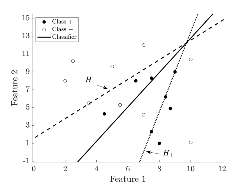
(a) Linear binary TPMSVM

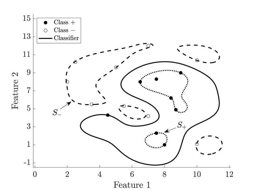
(b) Nonlinear binary TPMSVM

Figure 1: Linear and nonlinear classifiers for the case of binary TPMSVM. The parameters are $\nu_{+}=\nu_{-}=0.5$, $\alpha_{+}=\alpha_{-}=1$. In the nonlinear case, the Gaussian kernel with $\sigma=1.5$ is considered.

2.3 The nonlinear TPMSVM

In order to increase the predictive power of the model and include situations where observations are not linearly separable, in Peng (2011) the nonlinear extension of the TPMSVM is provided. In accordance with the classical approach of Cortes and Vapnik (1995), training data points are firstly mapped to a inner product space ($\mathcal{H}$, $\langle\cdot,\cdot\rangle$) via a feature map $\varphi:\mathbb{R}^{n}\to\mathcal{H}$. Then, their projected value are linearly classified in $\mathcal{H}$, by means of a SVM-type model.
Following this idea, hyperplanes $H_{+}$ and $H_{-}$ are now defined in the feature space $\mathcal{H}$ according to the equations:

$$H_{+}:\langle w_{+},\varphi(x)\rangle+\theta_{+}=0\qquad H_{-}:\langle w_{-},\varphi(x)\rangle+\theta_{-}=0,$$ (9)

with $w_{+},w_{-}\in\mathcal{H}$ and $\theta_{+},\theta_{-}\in\mathbb{R}$. Accordingly, models (2)-(3) are modified as:

$$\min_{w_{+},\theta_{+},\xi_{+}} \frac{1}{2}\langle w_{+},w_{+}\rangle+\frac{\nu_{+}}{m_{-}}\sum_{j\in\mathcal{X}_{-}}\big{(}\langle w_{+},\varphi(x^{j})\rangle+b_{+}\big{)}+\frac{\alpha_{+}}{m_{+}}e_{+}^{\top}\xi_{+}$$ (10)

s.t. $$\langle w_{+},\varphi(x^{i})\rangle+\theta_{+}\geq-\xi_{+,i}\qquad i\in\mathcal{X_{+}}$$

$$\xi_{+}\geq 0,$$

and

$$\min_{w_{-},\theta_{-},\xi_{-}} \frac{1}{2}\langle w_{-},w_{-}\rangle+\frac{\nu_{-}}{m_{+}}\sum_{i\in\mathcal{X}_{+}}\big{(}\langle w_{-},\varphi(x^{i})\rangle+b_{-}\big{)}+\frac{\alpha_{-}}{m_{-}}e_{-}^{\top}\xi_{-}$$ (11)

s.t. $$\langle w_{-},\varphi(x^{j})\rangle+\theta_{-}\leq\xi_{-,j}\qquad j\in\mathcal{X_{-}}$$

$$\xi_{-}\geq 0,$$

where $\xi_{+,i}$ and $\xi_{-,j}$ are the $i$-th and the $j$-th components of $\xi_{+}$ and $\xi_{-}$, respectively. The projections of the hyperplanes $H_{+}$ and $H_{-}$ from the feature space $\mathcal{H}$ onto the input space $\mathbb{R}^{n}$ are the corresponding separating surfaces $S_{+}$ and $S_{-}$.
Unfortunately, a closed-form expression of the feature map $\varphi(\cdot)$ is rarely available, and thus models (10)-(11) are not solvable in practice (see Jiménez-Cordero et al. (2021)). Nevertheless, it is possible to reformulate them by applying the so-called kernel trick (see Cortes and Vapnik (1995)). Indeed, a positive definite and symmetric kernel $k:\mathbb{R}^{n}\times\mathbb{R}^{n}\to\mathbb{R}$ is introduced such that $k(x,x^{\prime})=\langle\varphi(x),\varphi(x^{\prime})\rangle$, for all $x,x^{\prime}\in\mathbb{R}^{n}$. Examples of kernels typically used in the ML literature are reported in Table 1. The reader is referred to Schölkopf and Smola (2001) for a comprehensive overview on kernel functions.

Kernel function	$k(x,x^{\prime})$	Parameter
Homogeneous polynomial	$k(x,x^{\prime})=(x^{\top}x^{\prime})^{d}$	$d\in\mathbb{N}$
Inhomogeneous polynomial	$k(x,x^{\prime})=(\gamma+x^{\top}x^{\prime})^{d}$	$\gamma\geq 0$, $d\in\mathbb{N}$
Gaussian	$k(x,x^{\prime})=\exp\bigg{(}\displaystyle-\frac{\left\lVert x-x^{\prime}\right\rVert_{2}^{2}}{2\sigma^{2}}\bigg{)}$	$\sigma>0$
Sigmoid	$k(x,x^{\prime})=\tanh(a\text{ }x^{\top}x^{\prime}+b)$	$a\in\mathbb{R}$, $b\in\mathbb{R}$

Table 1: Examples of kernel functions.

The dual problems of (10) and (11) can be reformulated in terms of $k(\cdot,\cdot)$, namely:

$$\max_{\lambda_{+}} -\frac{1}{2}\lambda_{+}^{\top}K(X_{+},X_{+})\lambda_{+}+\frac{\nu_{+}}{m_{-}}e_{-}^{\top}K(X_{-},X_{+})\lambda_{+}$$ (12)

s.t. $$e_{+}^{\top}\lambda_{+}=\nu_{+}$$

$$0\leq\lambda_{+}\leq\frac{\alpha_{+}}{m_{+}},$$

and

$$\max_{\lambda_{-}} -\frac{1}{2}\lambda_{-}^{\top}K(X_{-},X_{-})\lambda_{-}+\frac{\nu_{-}}{m_{+}}e_{+}^{\top}K(X_{+},X_{-})\lambda_{-}$$ (13)

s.t. $$e_{-}^{\top}\lambda_{-}=\nu_{-}$$

$$0\leq\lambda_{-}\leq\frac{\alpha_{-}}{m_{-}},$$

where $K(X_{+},X_{+})$ is the matrix of the dot products $\langle\varphi(x^{i}),\varphi(x^{\widetilde{i}})\rangle$ for $i,\tilde{i}\in\mathcal{X_{+}}$. Similarly with $K(X_{+},X_{-})$, $K(X_{-},X_{+})$ and $K(X_{-},X_{-})$.
As in the linear case, once problems (4)-(5) are solved, the KKT conditions provide $(w_{+},\theta_{+})$ and $(w_{-},\theta_{-})$. Finally, they are combined in the decision function:

$$f_{\text{nonlin}}(x)=\operatorname{sign}\bigg{(}\frac{\langle w_{+},\varphi(x)\rangle+\theta_{+}}{\sqrt{\langle w_{+},w_{+}\rangle}}+\frac{\langle w_{-},\varphi(x)\rangle+\theta_{-}}{\sqrt{\langle w_{-},w_{-}\rangle}}\bigg{)}.$$ (14)

It is possible to reformulate the expression of $f_{\text{nonlin}}$ by explicitly considering the kernel $k(\cdot,\cdot)$.
In Figure 1(b) we depict the separating surfaces $S_{+}$ and $S_{-}$, along with the classifier $f_{\text{nonlin}}=0$, when the kernel is Gaussian with $\sigma=1.5$.

3 A novel multiclass TPMSVM-type model

In this section, we extend the binary TPMSVM to the case of multiclass classification, by considering a one-versus-all approach (see Xie et al. (2013)). We start with the linear case, and then we generalize the model to nonlinear classifiers.

3.1 The linear multiclass model

Similarly to the binary case, we denote by $\{x^{i},y_{i}\}_{i=1}^{m}$ the set of training data points. However, in this situation, label $y_{i}$ belongs to $\{1,\ldots,C\}$, where $C$ is the total number of classes. For each $c=1,\ldots,C$, let $m_{c}$ and $m_{-c}$ be the number of observations belonging to class $c$ and not to class $c$, respectively, such that $m_{c}+m_{-c}=m$. Matrix $X_{c}\in\mathbb{R}^{n\times m_{c}}$ represents all training data points of class $c$. Similarly, for matrix $X_{-c}\in\mathbb{R}^{n\times m_{-c}}$. The corresponding indices sets are $\mathcal{X}_{c}$ and $\mathcal{X}_{-c}$, respectively.
For each class $c=1,\ldots,C$ we aim to find the best separating hyperplane $H_{c}$ defined by equation $w_{c}^{\top}x+\theta_{c}=0$, where $w_{c}\in\mathbb{R}^{n}$ and $\theta_{c}\in\mathbb{R}$. In the spirit of the one-versus-all approach, $w_{c}$ and $\theta_{c}$ are the solutions of the following QPP:

$$\min_{w_{c},\theta_{c},\xi_{c}} \frac{1}{2}\left\lVert w_{c}\right\rVert_{2}^{2}+\frac{\nu_{c}}{m_{-c}}e_{-c}^{\top}\big{(}X_{-c}^{\top}w_{c}+e_{-c}\theta_{c}\big{)}+\frac{\alpha_{c}}{m_{c}}e_{c}^{\top}\xi_{c}$$ (15)

s.t. $$X_{c}^{\top}w_{c}+e_{c}\theta_{c}\geq-\xi_{c}$$

$$\xi_{c}\geq 0.$$

Model (15) is similar to (2). In the multiclass context, the positive class of model (2) is replaced by class $c$ and the negative class by all other classes. Within this choice, all the observations not in class $c$ are as far as possible from $H_{c}$. Parameters $\nu_{c}$ and $\alpha_{c}$ in model (15) have an equivalent explanation of the corresponding ones in model (2).
By introducing the Lagrangian function of problem (15) and by applying the KTT conditions, the dual problem is given by:

$$\max_{\lambda_{c}} -\frac{1}{2}\lambda_{c}^{\top}X_{c}^{\top}X_{c}\lambda_{c}+\frac{\nu_{c}}{m_{-c}}e_{-c}^{\top}X_{-c}^{\top}X_{c}\lambda_{c}$$ (16)

s.t. $$e_{c}^{\top}\lambda_{c}=\nu_{c}$$

$$0\leq\lambda_{c}\leq\frac{\alpha_{c}}{m_{c}},$$

with optimal solutions

$$w_{c}=X_{c}\lambda_{c}-\frac{\nu_{c}}{m_{-c}}X_{-c}e_{-c}\qquad\theta_{c}=-\frac{1}{\lvert{\mathcal{N}_{c}}\rvert}\sum_{i\in\mathcal{N}_{c}}{x^{i}}^{\top}w_{c}.$$ (17)

Once all the $C$ hyperplanes have been determined, we consider the following decision function:

$$f_{\text{lin},C,\min}(x):=\operatorname*{arg\,min}_{c=1,\ldots,C}\frac{\left\lvert w_{c}^{\top}x+\theta_{c}\right\rvert}{\left\lVert w_{c}\right\rVert_{2}}.$$ (18)

3.2 The nonlinear multiclass model

When dealing with nonlinear classifier, kernel-induced decision boundary $S_{c}$ is defined by equation $\langle w_{c},\varphi(x)\rangle+\theta_{c}=0$ for class $c=1,\ldots,C$. The kernel trick (Cortes and Vapnik (1995)) applied to problem (16) leads to:

$$\max_{\lambda_{c}} -\frac{1}{2}\lambda_{c}^{\top}K(X_{c},X_{c})\lambda_{c}+\frac{\nu_{c}}{m_{-c}}e_{-c}^{\top}K(X_{-c},X_{c})\lambda_{c}$$ (19)

s.t. $$e_{c}^{\top}\lambda_{c}=\nu_{c}$$

$$0\leq\lambda_{c}\leq\frac{\alpha_{c}}{m_{c}},$$

where $K(X_{c},X_{c})$ is the $m_{c}\times m_{c}$ matrix with entries $\langle\varphi(x^{i}),\varphi(x^{\widetilde{i}})\rangle$ for $i,\tilde{i}\in\mathcal{X}_{c}$. Similarly with $K(X_{-c},X_{c})$. The KKT conditions provide the optimal solutions $(w_{c},\theta_{c})$, leading to the following classifier:

$$f_{\text{nonlin},C,\min}(x):=\operatorname*{arg\,min}_{c=1,\ldots,C}\frac{\left\lvert\langle w_{c},\varphi(x)\rangle+\theta_{c}\right\rvert}{\sqrt{\langle w_{c},w_{c}\rangle}},$$ (20)

where, for all $c=1,\ldots,C$,

$$\langle w_{c},\varphi(x)\rangle=\lambda_{c}^{\top}K(X_{c},x)-\frac{\nu_{c}}{m_{-c}}e_{-c}^{\top}K(X_{-c},x),$$

$$\theta_{c}=-\frac{1}{\lvert{\mathcal{N}_{c}}\rvert}\sum_{i\in\mathcal{N}_{c}}\big{[}K(x^{i},X_{c})\lambda_{c}-\frac{\nu_{c}}{m_{-c}}K(x^{i},X_{-c})e_{-c}\big{]},$$

and

$$\begin{split}\langle w_{c},\varphi(x)\rangle&=\lambda_{c}^{\top}K(X_{c},X_{c})\lambda_{c}-\frac{\nu_{c}}{m_{-c}}\lambda_{c}^{\top}K(X_{c},X_{-c})e_{-c}+\\ &-\frac{\nu_{c}}{m_{-c}}e_{-c}^{\top}K(X_{-c},X_{c})\lambda_{c}+\frac{\nu_{c}^{2}}{m_{-c}^{2}}e_{-c}^{\top}K(X_{-c},X_{-c})e_{-c}.\end{split}$$

4 The robust model

In this section, we derive the robust counterpart of model (15). We start by assuming that each observation $x^{i}$ is subject to an unknown but bounded by $\ell_{p}$-norm perturbation $\delta^{i}$ (see Trafalis and Gilbert (2006)). Specifically, the uncertainty set around $x^{i}$ has the following expression:

$$\mathcal{U}_{p}(x^{i}):=\big{\{}x\in\mathbb{R}^{n}\lvert x=x^{i}+\delta^{i},\left\lVert\delta^{i}\right\rVert_{p}\leq\varepsilon_{i}\big{\}},$$ (21)

where $p\in[1,+\infty]$ and $\varepsilon_{i}\geq 0$. The value of the radius $\varepsilon_{i}$ controls the degree of conservatism. When $\varepsilon_{i}=0$, the uncertainty set $\mathcal{U}_{p}(x^{i})$ reduces to its center $x^{i}$.

4.1 The robust model for linear multiclass classification

Robustifying model (15) against the uncertainty set $\mathcal{U}_{p}(x^{i})$ yields the following optimization model:

$$\min_{w_{c},\theta_{c},\xi_{c}} \frac{1}{2}\left\lVert w_{c}\right\rVert_{2}^{2}+\frac{\nu_{c}}{m_{-c}}\sum_{i\in\mathcal{X}_{-c}}\max_{\left\lVert\delta^{i}\right\rVert_{p}\leq\varepsilon_{i}}\big{[}\big{(}x^{i^{\top}}+\delta^{i^{\top}}\big{)}w_{c}+\theta_{c}\big{]}+\frac{\alpha_{c}}{m_{c}}\sum_{i\in\mathcal{X}_{c}}\xi_{c,i}$$ (22)

s.t. $$x^{\top}w_{c}+\theta_{c}\geq-\xi_{c,i}\qquad i\in\mathcal{X}_{c},\forall x\in\mathcal{U}_{p}(x^{i})$$

$$\xi_{c,i}\geq 0\qquad i\in\mathcal{X}_{c}.$$

Since there exists infinite possibilities for choosing $x\in\mathcal{U}_{p}(x^{i})$, model (22) is intractable. In the following theorem, a tractable closed-form expression is derived.

Theorem 1.

Let $\mathcal{U}_{p}(x^{i})$ be the uncertainty set as in (21), with $p\in[1,\infty]$. Let $p^{\prime}$ be the Hölder conjugate of $p$, namely $1/p+1/p^{\prime}=1$. The robust counterpart of model (15) is:

$$\min_{w_{c},\theta_{c},\xi_{c}} \frac{1}{2}\left\lVert w_{c}\right\rVert_{2}^{2}+\frac{\nu_{c}}{m_{-c}}\sum_{i\in\mathcal{X}_{-c}}\big{(}x^{i^{\top}}w_{c}+\varepsilon_{i}\left\lVert w_{c}\right\rVert_{p^{\prime}}\big{)}+\nu_{c}\theta_{c}+\frac{\alpha_{c}}{m_{c}}\sum_{i\in\mathcal{X}_{c}}\xi_{c,i}$$ (23)

s.t. $$x^{i^{\top}}w_{c}+\theta_{c}-\varepsilon_{i}\left\lVert w_{c}\right\rVert_{p^{\prime}}\geq-\xi_{c,i}\qquad i\in\mathcal{X}_{c}$$

$$\xi_{c,i}\geq 0\qquad i\in\mathcal{X}_{c}.$$

Proof.

Model (22) can be expressed as (see Bertsimas et al. (2019)):

$$\min_{w_{c},\theta_{c},\xi_{c}} \frac{1}{2}\left\lVert w_{c}\right\rVert_{2}^{2}+\frac{\nu_{c}}{m_{-c}}\sum_{i\in\mathcal{X}_{-c}}\max_{\left\lVert\delta^{i}\right\rVert_{p}\leq\varepsilon_{i}}\big{[}\big{(}x^{i^{\top}}+\delta^{i^{\top}}\big{)}w_{c}+\theta_{c}\big{]}+\frac{\alpha_{c}}{m_{c}}\sum_{i\in\mathcal{X}_{c}}\xi_{c,i}$$ (24)

s.t. $$\min_{\left\lVert\delta^{i}\right\rVert_{p}\leq\varepsilon_{i}}\big{[}\big{(}x^{i^{\top}}+\delta^{i^{\top}}\big{)}w_{c}\big{]}+\theta_{c}\geq-\xi_{c,i}\qquad i\in\mathcal{X}_{c}$$

$$\xi_{c,i}\geq 0\qquad i\in\mathcal{X}_{c}.$$

The maximization term in the objective function corresponds to:

$$\frac{\nu_{c}}{m_{-c}}\sum_{i\in\mathcal{X}_{-c}}\max_{\left\lVert\delta^{i}\right\rVert_{p}\leq\varepsilon_{i}}\big{[}x^{i^{\top}}w_{c}+\delta^{i^{\top}}w_{c}+\theta_{c}\big{]}=\nu_{c}\theta_{c}+\frac{\nu_{c}}{m_{-c}}\sum_{i\in\mathcal{X}_{-c}}\bigg{(}x^{i^{\top}}w_{c}+\max_{\left\lVert\delta^{i}\right\rVert_{p}\leq\varepsilon_{i}}\big{[}\delta^{i^{\top}}w_{c}\big{]}\bigg{)}.$$

By definition of the dual norm (see Rudin (1987)), we get:

$$\max_{\left\lVert\delta^{i}\right\rVert_{p}\leq\varepsilon_{i}}{\delta^{i^{\top}}w_{c}}=\varepsilon_{i}\left\lVert w_{c}\right\rVert_{p^{\prime}},$$

where $p^{\prime}$ is the Hölder conjugates of $p$. This implies that

$$-\varepsilon_{i}\left\lVert w_{c}\right\rVert_{p^{\prime}}\leq\delta^{i^{\top}}w_{c}\leq\varepsilon_{i}\left\lVert w_{c}\right\rVert_{p^{\prime}}.$$ (25)

Consequently, the second term in the objective function of (24) corresponds to:

$$\nu_{c}\theta_{c}+\frac{\nu_{c}}{m_{-c}}\sum_{i\in\mathcal{X}_{-c}}\bigg{(}x^{i^{\top}}w_{c}+\varepsilon_{i}\left\lVert w_{c}\right\rVert_{p^{\prime}}\bigg{)}.$$

As far as it concerns the first set of constraints in (24), for all $i\in\mathcal{X}_{c}$ it can be expressed as:

$$\min_{\left\lVert\delta^{i}\right\rVert_{p}\leq\varepsilon_{i}}\big{[}\delta^{i^{\top}}w_{c}\big{]}\geq-\xi_{c,i}-\theta_{c}-x^{i^{\top}}w_{c}.$$

By considering the first inequality in (25), the previous problem can be solved as

$$x^{i^{\top}}w_{c}+\theta_{c}-\varepsilon_{i}\left\lVert w_{c}\right\rVert_{p^{\prime}}\geq-\xi_{c,i}.$$

This concludes the proof. ∎

If no uncertainty occurs, $\varepsilon_{i}=0$ and thus the robust model (23) reduces to the deterministic model (15). In addition, model (23) is a convex nonlinear optimization model due to the presence of the $\ell_{2}$- and $\ell_{p^{\prime}}$-norm of $w_{c}$. The quadratic term $\left\lVert w_{c}\right\rVert_{2}^{2}$ can be easily transformed from the objective function to the constraints by introducing auxiliary variables $t_{c},u_{c},v_{c}\in\mathbb{R}$ (see Qi et al. (2013)), leading to:

$$\min_{w_{c},\theta_{c},\xi_{c},t_{c},u_{c},v_{c}} \frac{1}{2}(u_{c}-v_{c})+\frac{\nu_{c}}{m_{-c}}\sum_{i\in\mathcal{X}_{-c}}\big{(}x^{i^{\top}}w_{c}+\varepsilon_{i}\left\lVert w_{c}\right\rVert_{p^{\prime}}\big{)}+\nu_{c}\theta_{c}+\frac{\alpha_{c}}{m_{c}}\sum_{i\in\mathcal{X}_{c}}\xi_{c,i}$$ (26)

s.t. $$x^{i^{\top}}w_{c}+\theta_{c}-\varepsilon_{i}\left\lVert w_{c}\right\rVert_{p^{\prime}}\geq-\xi_{c,i}\qquad i\in\mathcal{X}_{c}$$

$$t_{c}\geq\left\lVert w_{c}\right\rVert_{2}$$

$$u_{c}+v_{c}=1$$

$$u_{c}\geq\sqrt{t_{c}^{2}+v_{c}^{2}}$$

$$\xi_{c,i}\geq 0\qquad i\in\mathcal{X}_{c}.$$

In the cases of box, polyhedral and spherical uncertainty sets (El Ghaoui et al. (2003), López et al. (2019), Fan et al. (2014)), model (26) reduces to a SOCP problem, as stated in the following result.

Corollary 1.

Let $\mathcal{U}_{p}(x^{i})$ be the uncertainty set as in (21). Model (26) can be expressed as a SOCP problem in the following cases:

• Case $p=1$:

  $$\min_{w_{c},\theta_{c},\xi_{c},t_{c},u_{c},v_{c},s_{c}} \frac{1}{2}(u_{c}-v_{c})+\frac{\nu_{c}}{m_{-c}}\sum_{i\in\mathcal{X}_{-c}}\big{(}x^{i^{\top}}w_{c}+\varepsilon_{i}s_{c}\big{)}+\nu_{c}\theta_{c}+\frac{\alpha_{c}}{m_{c}}\sum_{i\in\mathcal{X}_{c}}\xi_{c,i}$$ (27)

  s.t. $$x^{i^{\top}}w_{c}+\theta_{c}-\varepsilon_{i}s_{c}\geq-\xi_{c,i}\qquad i\in\mathcal{X}_{c}$$

  $$t_{c}\geq\left\lVert w_{c}\right\rVert_{2}$$

  $$u_{c}+v_{c}=1$$

  $$u_{c}\geq\sqrt{t_{c}^{2}+v_{c}^{2}}$$

  $$s_{c}\geq-w_{c,j}\qquad j=1,\ldots,n$$

  $$s_{c}\geq w_{c,j}\qquad j=1,\ldots,n$$

  $$s_{c}\geq 0$$

  $$\xi_{c,i}\geq 0\qquad i\in\mathcal{X}_{c}.$$

• Case $p=2$:

  $$\min_{w_{c},\theta_{c},\xi_{c},t_{c},u_{c},v_{c}} \frac{1}{2}(u_{c}-v_{c})+\frac{\nu_{c}}{m_{-c}}\sum_{i\in\mathcal{X}_{-c}}\big{(}x^{i^{\top}}w_{c}+\varepsilon_{i}t_{c}\big{)}+\nu_{c}\theta_{c}+\frac{\alpha_{c}}{m_{c}}\sum_{i\in\mathcal{X}_{c}}\xi_{c,i}$$ (28)

  s.t. $$x^{i^{\top}}w_{c}+\theta_{c}-\varepsilon_{i}t_{c}\geq-\xi_{c,i}\qquad i\in\mathcal{X}_{c}$$

  $$t_{c}\geq\left\lVert w_{c}\right\rVert_{2}$$

  $$u_{c}+v_{c}=1$$

  $$u_{c}\geq\sqrt{t_{c}^{2}+v_{c}^{2}}$$

  $$\xi_{c,i}\geq 0\qquad i\in\mathcal{X}_{c}.$$

• Case $p=\infty$:

  $$\min_{w_{c},\theta_{c},\xi_{c},t_{c},u_{c},v_{c},s_{c}} \frac{1}{2}(u_{c}-v_{c})+\frac{\nu_{c}}{m_{-c}}\sum_{i\in\mathcal{X}_{-c}}\big{(}x^{i^{\top}}w_{c}+\varepsilon_{i}\sum_{j=1}^{n}s_{c,j}\big{)}+\nu_{c}\theta_{c}+\frac{\alpha_{c}}{m_{c}}\sum_{i\in\mathcal{X}_{c}}\xi_{c,i}$$ (29)

  s.t. $$x^{i^{\top}}w_{c}+\theta_{c}-\varepsilon_{i}\sum_{j=1}^{n}s_{c,j}\geq-\xi_{c,i}\qquad i\in\mathcal{X}_{c}$$

  $$t_{c}\geq\left\lVert w_{c}\right\rVert_{2}$$

  $$u_{c}+v_{c}=1$$

  $$u_{c}\geq\sqrt{t_{c}^{2}+v_{c}^{2}}$$

  $$s_{c,j}\geq-w_{c,j}\qquad j=1,\ldots,n$$

  $$s_{c,j}\geq w_{c,j}\qquad j=1,\ldots,n$$

  $$\xi_{c,i}\geq 0\qquad i\in\mathcal{X}_{c}.$$

Proof.

The proof is similar to that present in Section 2.4 and 2.5 in Trafalis and Gilbert (2006). ∎

For a general analysis of the case of $p\in(1,+\infty)$, the reader is referred to Blanco et al. (2020).

5 Preliminary numerical results

In this section, we investigate the performance of the proposed TPMSVM-type approach for a multiclass classification task. We consider 2 real-world multiclass datasets from the UCI Machine Learning repository (see Dua and Graff (2017)). Their summary statistics are reported in Table 2. All models are implemented in MATLAB (version 2021b) and numerical results are obtained using MOSEK solver (version 9.1.9). Computational experiments are run on a MacBookPro17.1 with a chip Apple M1 of 8 cores and 16 GB of RAM memory.

Dataset	Source	Application Field	Observations	Features	Classes
Iris	UCI	Life Sciences	150	4	3
Wine	UCI	Physical Sciences	178	13	3

Table 2: Summary statistics of considered datasets.

Each dataset is split into training set and testing set, with a proportion of 75%-25% of the total number of observations. The partition is performed according to the proportional random sampling strategy (see Chen et al. (2001), implying that the original class balance in the entire dataset is maintained both in the training and in the testing set. In order to avoid imbalances among the orders of magnitude of the features (Han et al. (2011)), before training each dataset is normalized such that the features are linearly scaled into the unit interval $[0,1]$. As far as it concerns hyperparameters in models (16) and (19), for simplicity we set $\nu_{c}=\nu$ and $\alpha_{c}=\alpha$ for all $c=1,\ldots,C$. A grid search procedure (Yu and Zhu (2020)) is applied to tune their values. Specifically, $\alpha$ is selected from the set $\{2^{j}|j=-8,-7,\ldots,7,8\}$, whereas, as in Peng (2011), the value of $\nu/\alpha$ is chosen from the set $\{0.1,0.2,\ldots,0.8,0.9\}$. The parameters $\gamma$ for the inhomogeneous polynomial kernel and $\sigma$ for the Gaussian kernel takes value in $\{2^{j}|j=-4,-3,\ldots,3,4\}$. The best configuration of parameters is selected as the one maximizing the accuracy of the model on the training set. Once it is determined, the model is tested on the training set and the corresponding accuracy is computed. In order to get stable results, for each hold-out 75%-25% the computational experiments are performed over 100 different combinations of training and testing set, and results are then averaged.
Table 3 reports the results of deterministic models (15) and (19) in terms of mean accuracy and standard deviations. The CPU time for training the model is outlined below each result.

Dataset			Kernel
		Linear	Hom. quadratic	Hom. cubic	Inhom. linear	Inhom. quadratic	Inhom. cubic	Gaussian
Iris	Accuracy	$\mathbf{92.08\pm 3.71}$	$75.27\pm 4.97$	$85.51\pm 4.55$	${91.76\pm 3.92}$	$91.62\pm 3.83$	$88.78\pm 5.40$	$90.70\pm 4.71$
	CPU time (s)	101.27	673.58	657.31	4242.87	6533.84	6658.95	13051.45
Wine	Accuracy	$\mathbf{97.02\pm 2.28}$	$96.41\pm 2.69$	$95.70\pm 2.85$	$96.34\pm 2.70$	$96.35\pm 2.24$	to be done	to be done
	CPU time (s)	101.56	2059.08	2119.25	10768.81	19982.60

Table 3: Detailed percentage results of average accuracy and standard deviation over 100 runs of the deterministic models (15) and (19). The best result is in bold.

6 Conclusions and future works

In this paper we have proposed a novel TPMSVM-type model for classification. We have extended the results in the literature to the multiclass context, in both the cases of linear and nonlinear classifier. We have derived the robust counterpart of the models by considering a general bounded-by-$\ell_{p}$-norm uncertainty set around each input data. This allows to increase the flexibility of the model, depending on the quality of the observations. Preliminary numerical results show the good performance of the proposed methodology in the deterministic case.
The work is in progress and in the short term we will deal with the following aspects. From the methodological perspective, we will derive the dual problems of models (27)-(29), and consider the robust counterpart of model (19), in order to include kernel-induced decision boundaries. We will consider different decision functions, depending on max voting strategies or max distance too. On the other hand, as far as it concerns the computational results, we will test the models on several real-world datasets, both in the deterministic and robust cases. We will compare the outcomes with models in the literature.

References

References

• Angulo et al. (2003) Angulo, C., Parra, X., Català, A., 2003. K-svcr. a support vector machine for multi-class classification. Neurocomputing 55, 57–77.
• Arun Kumar and Gopal (2009) Arun Kumar, M., Gopal, M., 2009. Least squares twin support vector machines for pattern classification. Expert Systems with Applications 36, 7535–43.
• Bertsimas et al. (2019) Bertsimas, D., Dunn, J., Pawlowski, C., Zhuo, Y.D., 2019. Robust classification. INFORMS Journal of Optimization 1, 2–34.
• Blanco et al. (2020) Blanco, V., Puerto, J., Rodríguez-Chía, A.M., 2020. On lp-support vector machines and multidimensional kernels. Journal of Machine Learning Research 21, 1–29.
• Boser et al. (1992) Boser, B.E., Guyon, I., Vapnik, V.N., 1992. A training algorithm for optimal margin classifiers. Proceedings of the Fifth Annual Workshop of Computational Learning Theory 5, 144–52.
• Bredensteiner and Bennett (1999) Bredensteiner, E.J., Bennett, K.P., 1999. Multicategory classification by support vector machines. Computational Optimization and Applications 12, 53–79.
• Chen et al. (2001) Chen, T.Y., Tse, T.H., Yu, Y.T., 2001. Proportional sampling strategy: a compendium and some insights. The Journal of Systems and Software 58, 65–81.
• Chen et al. (2011) Chen, X., Yang, J., Ye, Q., Liang, J., 2011. Recursive projection twin support vector machine via within-class variance minimization. Pattern Recognition 44, 2643–55.
• Cortes and Vapnik (1995) Cortes, C., Vapnik, V.N., 1995. Support-vector networks. Machine Learning 20, 273–97.
• Ding et al. (2019) Ding, S., Zhao, X., Zhang, J., Zhang, X., Xue, Y., 2019. A review on multi-class twsvm. Artificial Intelligence Review 52, 775–801.
• Du et al. (2021) Du, S.W., Zhang, M.C., Chen, P., Sun, H.F., Chen, W.J., Shao, Y.H., 2021. A multiclass nonparallel parametric-margin support vector machine. Information 12, 515–33.
• Dua and Graff (2017) Dua, D., Graff, C., 2017. UCI machine learning repository. URL: http://archive.ics.uci.edu/ml.
• El Ghaoui et al. (2003) El Ghaoui, L., Lanckriet, G.R.G., Natsoulis, G., 2003. Robust classification with interval data. Technical Report UCB/CSD-03-1279, EECS Department, University of California, Berkeley .
• Faccini et al. (2022) Faccini, D., Maggioni, F., Potra, F.A., 2022. Robust and distributionally robust optimization models for linear support vector machine. Computers and Operations Research 147, 105930.
• Fan et al. (2014) Fan, N., Sadeghi, E., Pardalos, P.M., 2014. Robust support vector machines with polyhedral uncertainty of the input data, in: Learning and Intelligent Optimization. International Conference on Learning and Intelligent Optimization, Springer-Verlag. pp. 291–305.
• Han et al. (2011) Han, J., Kamber, M., Pei, J., 2011. Data mining: concepts and techniques - 3rd edition. Morgan Kaufmann.
• Hao (2010) Hao, P.Y., 2010. New support vector algorithms with parametric insensitive/margin model. Neural networks : the official journal of the International Neural Network Society 23, 60–73.
• Hastie and Tibshirani (1998) Hastie, T., Tibshirani, R., 1998. Classification by pairwise coupling. The Annals of Statistics 26, 451 –71.
• Jayadeva et al. (2007) Jayadeva, Khemchandani, R., Chandra, S., 2007. Twin support vector machines for pattern classification. IEEE Transactions on Pattern Analysis and Machine Intelligence 29, 905–10.
• Jiménez-Cordero et al. (2021) Jiménez-Cordero, A., Morales, J.M., Pineda, S., 2021. A novel embedded min-max approach for feature selection in nonlinear support vector machine classification. European Journal of Operational Research 293, 24–35.
• Liu and Potra (2009) Liu, X., Potra, F.A., 2009. Pattern separation and prediction via linear and semidefinite programming. Studies in Informatics and Control 18, 71–82.
• López et al. (2019) López, J., Maldonado, S., Carrasco, M., 2019. Robust nonparallel support vector machines via second-order cone programming. Neurocomputing 364, 227–38.
• Maggioni and Spinelli (2023) Maggioni, F., Spinelli, A., 2023. A robust optimization model for nonlinear support vector machine. In preparation .
• Peng (2011) Peng, X., 2011. Tpmsvm: A novel twin parametric-margin support vector machine for pattern recognition. Pattern Recognition 44, 2678–92.
• Peng and Xu (2013) Peng, X., Xu, D., 2013. Robust minimum class variance twin support vector machine classifier. Neural Computing and Applications 22, 999–1011.
• Platt et al. (1999) Platt, J., Cristianini, N., Shawe-Taylor, J., 1999. Large margin dags for multiclass classification, in: Solla, S., Leen, T., Müller, K. (Eds.), Advances in Neural Information Processing Systems, MIT Press. pp. 547–53.
• Qi et al. (2013) Qi, Z., Tian, Y., Shi, Y., 2013. Robust twin support vector machine for pattern classification. Pattern Recognition 46, 305–16.
• Rudin (1987) Rudin, W., 1987. Real and complex analysis. McGraw-Hill.
• Schölkopf et al. (2000) Schölkopf, B., Smola, A., Williamson, R.C., Bartlett, P.L., 2000. New support vector algorithms. Neural Computation 12, 1207–45.
• Schölkopf and Smola (2001) Schölkopf, B., Smola, A.J., 2001. Learning with Kernels: Support Vector Machines, regularization, optimization, and beyond. MIT press.
• Shao et al. (2013) Shao, Y.H., Chen, W.J., Huang, W.B., Yang, Z.M., Deng, N.Y., 2013. The best separating decision tree twin support vector machine for multi-class classification. Procedia Computer Science 17, 1032–8.
• Shapiro et al. (2009) Shapiro, A., Dentcheva, D., Ruszczynski, A., 2009. Lectures on Stochastic Programming - Modeling and Theory. MOS-SIAM Series on Optimization.
• Tanveer et al. (2022) Tanveer, M., Rajani, T., Rastogi, R., Shao, Y., 2022. Comprehensive review on twin support vector machines. Annals of Operations Research .
• Trafalis and Gilbert (2006) Trafalis, T.B., Gilbert, R.C., 2006. Robust classification and regression using support vector machines. European Journal of Operational Research 173, 893–909.
• Vapnik (1982) Vapnik, V.N., 1982. Estimation of dependences based on empirical data. Springer-Verlag.
• Vapnik (1995) Vapnik, V.N., 1995. The nature of statistical learning theory. Springer-Verlag.
• Xie et al. (2013) Xie, J., Hone, K.S., Xie, W., Gao, X., Shi, Y., Liu, X., 2013. Extending twin support vector machine classifier for multi-category classification problems. Intelligent Data Analysis 17, 649–64.
• Xu et al. (2009) Xu, H., Caramanis, C., Mannor, S., 2009. Robustness and regularization of support vector machines. Journal of Machine Learning Research 10, 1485–510.
• Xu et al. (2017) Xu, Y., Yang, Z., Pan, X., 2017. A novel twin support-vector machine with pinball loss. IEEE Transactions on Neural Networks and Learning Systems 28, 359–70.
• Yajima (2005) Yajima, Y., 2005. Linear programming approaches for multicategory support vector machines. European Journal of Operational Research 162, 514–31.
• Yang et al. (2013) Yang, Z., Shao, Y., Zhang, X.S., 2013. Multiple birth support vector machine for multi-class classification. Neural Computing and Applications 22, 153–61.
• Yu and Zhu (2020) Yu, T., Zhu, H., 2020. Hyper-parameter optimization: A review of algorithms and applications. arXiv:2003.05689.
• Zhong and Fukushima (2007) Zhong, P., Fukushima, M., 2007. Second-order cone programming formulations for robust multiclass classification. Neural Computation 19, 258--82.