Single-Model Attribution of Generative Models Through Final-Layer Inversion

Abstract

Recent breakthroughs in generative modeling have sparked interest in practical single-model attribution. Such methods predict whether a sample was generated by a specific generator or not, for instance, to prove intellectual property theft. However, previous works are either limited to the closed-world setting or require undesirable changes to the generative model. We address these shortcomings by, first, viewing single-model attribution through the lens of anomaly detection. Arising from this change of perspective, we propose FLIPAD, a new approach for single-model attribution in the open-world setting based on final-layer inversion and anomaly detection. We show that the utilized final-layer inversion can be reduced to a convex lasso optimization problem, making our approach theoretically sound and computationally efficient. The theoretical findings are accompanied by an experimental study demonstrating the effectiveness of our approach and its flexibility to various domains.

1 Introduction

Deep generative models have taken a giant leap forward in recent years; humans are not able to distinguish real and synthetic images anymore (Nightingale and Farid 2022; Mink et al. 2022; Lago et al. 2022), and text-to-image models like DALL-E 2 (Ramesh et al. 2022), Imagen (Saharia et al. 2022), and Stable Diffusion (Rombach et al. 2022) have sparked a controversial debate about AI-generated art (Rea 2023). But this superb performance comes, quite literally, at a price: besides technical expertise and dedication, large training datasets and enormous computational resources are needed. For instance, the training of the large-language model GPT-3 (Brown et al. 2020) is estimated to cost almost five million US dollars (Li 2020). Trained models have become valuable company assets—and an attractive target for intellectual-property theft. An interesting task is, therefore, to attribute a given sample to the generative model that created it.

Existing solutions to this problem can be divided into two categories: fingerprinting methods (e.g., Marra et al. 2019a; Yu, Davis, and Fritz 2019) exploit the fact that most synthetic samples contain generator-specific traces that a classifier can use to assign a sample to its corresponding source. Inversion methods (Albright and McCloskey 2019; Zhang et al. 2021; Hirofumi et al. 2022), on the other hand, are based on the idea that a synthetic sample can be reconstructed most accurately by the generator that created it. However, both approaches are designed for the closed-world setting, which means that they are designed to differentiate between models from a given set that is chosen before training and stays fixed during inference. In practice, this is rarely the case, since new models keep emerging. For detecting intellectual property theft, the setting of single-model attribution is more suitable. Here, the task is to determine whether a sample was created by one particular generative model or not, in the open-world setting. Previous work has found that this problem can be solved by complementing the model with a watermark that can be extracted from generated samples (Yu et al. 2021; Kim, Ren, and Yang 2021; Yu et al. 2022). Although watermarking has shown to be very effective, a major disadvantage is that it has to be incorporated into the training process, which a) might not always be desirable or even possible and b) can deteriorate generation quality.

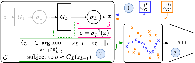
Figure 1: Single-model attribution with FLIPAD. Given a generative model $G$, FLIPAD performs the following steps: 1) The training data includes generated samples $x_{G}^{(i)}$ from $G$ and samples from a different source $x^{(i)}_{G’}$. For each $x$ we compute the optimization target $o$ by inverting the final activation $\sigma_{L}$. 2) For each output $o$, we perform final-layer inversion by finding an activation $\hat{z}_{L-1}$ that is close to the expected activation $\bar{z}_{L-1}$ and an approximate solution to $o\approx G_{L}(\hat{z}_{L-1})$. 3) Since final-layer inversion reveals differences between different data sources, the activations can be used as features to train an anomaly detector.

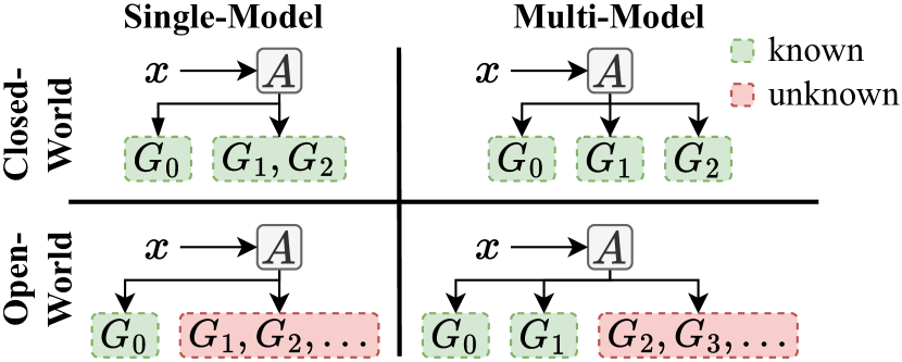
Figure 2: The two dimensions of the model attribution problem. Let $A$ be the attribution method. While single-model attribution solves a binary decision problem ($G_{0}$ or something else?), multi-model attribution can distinguish between more than two classes. In an open-world setting, it is also possible that a sample stems from an unknown generator.

In this work, we tackle the problem of single-model attribution in the open-world setting by viewing it as an anomaly detection task, which has not been done in previous works. This novel viewpoint motivates two simple, yet effective, baselines for the single-model attribution task. Furthermore, we find that incorporating knowledge about the generative model can improve the attribution accuracy and robustness. Specifically, we propose Final-Layer Inversion Plus Anomaly Detection (FLIPAD). First, it extracts meaningful features by leveraging the available model parameters to perform final-layer inversion. Second, it uses established anomaly detection techniques on the extracted features to predict whether a sample was generated by our generative model. While related to existing attribution methods based on inversion, our method is i) significantly more efficient due to the convexity of the optimization problem and ii) theoretically sound given the connection to the denoising basis pursuit. We highlight that this approach can be performed without altering the training process of the generative model. Moreover, it is not limited to the image domain since features are directly related to the generative process and do not exploit visual characteristics like frequency artifacts. We illustrate FLIPAD in Figure 1.

Our contributions are summarized as follows:

• We address the problem of single-model attribution in the open-world setting, which previously has not been solved adequately. Our work is the first to establish the natural connection between single-model attribution and anomaly detection. This change of perspective motivates two baseline methods, RawPAD and DCTPAD.

• Building upon on these baselines, we introduce FLIPAD, which combines final-layer inversion and anomaly detection. We prove that the proposed inversion scheme can be reframed as a convex lasso optimization problem, which makes it theoretically sound and computationally efficient.

• In an empirical analysis, we show the effectiveness and versatility of the proposed methods for a range of generative models, including GANs and diffusion models. Notably, our approach is not limited to the image domain.

2 Problem Setup

We consider the problem of model attribution to have two fundamental dimensions, which are illustrated in Figure 2. First, we differentiate between single-model and multi-model attribution. While in multi-model attribution the task is to find out by which specific generator (of a given set) a sample was created, single-model attribution only cares about whether a sample stems from a single model of interest or not. Note that, conceptually, real samples can be considered to be generated by a model as well, and thus, the task of distinguishing fake from real samples also fits into this framework. Second, attribution can be performed in the closed-world or open-world setting. The requirement for the closed-world setting is that all generators which could have generated the samples are known beforehand. In contrast, in the open-world setting an attribution method is able to state that the sample was created by an unknown generator.

The method proposed in this work solves the problem of single-model attribution in the open-world setting. Naturally, this setting applies for model creators interested in uncovering illegitimate usage of their model (or samples generated by it). In this scenario, FLIPAD only requires resources that are already available to the model creator: the model $G$ itself (including its parameters), samples $x_{G}$ generated by $G$, and real samples $x_{\operatorname{real}}$ used to train $G$. We emphasize that no samples generated by other models are needed. Therefore, we do not rely on restrictive data acquisition procedures, which might involve i) using additional computational resources to train models or sample new data, ii) expensive API calls, or iii) access to models that are kept private.

3 Related Work

We divide the existing work on deepfake attribution into three areas: fingerprinting, inversion, and watermarking. Regarding the problem setup, methods based on fingerprinting and inversion perform multi-model attribution in the open-world setting, while watermarking provides single-model attribution in the open-world setting. Note that all existing methods are designed for image data. A categorization of the related work is given in Appendix A.

Fingerprinting

The existence of fingerprints in GAN-generated images was demonstrated first by Marra et al. (2019a). They show that by averaging the noise residuals of generated images, different models can be distinguished based on the correlation coefficient between the image of interest and a set of model-specific fingerprints. Other works show that the accuracy can be improved by training an attribution network (Yu, Davis, and Fritz 2019) or extracting fingerprints in the frequency domain (Frank et al. 2020). Since fingerprinting only works in closed-world settings, methods to efficiently extend the set of known models (without expensive re-training) have been proposed (Marra et al. 2019b; Xuan et al. 2019).

Inversion

Inversion-based attribution is based on the finding that an image can be reconstructed by the generator that it originates from. While existing works (Albright and McCloskey 2019; Karras et al. 2020; Zhang et al. 2021; Hirofumi et al. 2022) prove that this approach is effective, it is computationally expensive since the optimal reconstruction has to be found iteratively using backpropagation. Additionally, since there is no guaranteed convergence due to the non-convexity of the optimization problem, multiple reconstruction attempts are necessary for each image.

Watermarking

Watermarking methods solve the attribution problem by proactively altering the generative model such that all generated images include a recognizable identifier. Yu et al. (2021) were the first to watermark GANs by encoding a visually imperceptible fingerprint into the training dataset. Generated images can be attributed by checking the decoded fingerprint. In a follow-up work (Yu et al. 2022), the authors propose a mechanism for embedding fingerprints more efficiently by directly embedding them into the model’s convolutional filters. A related work by Kim, Ren, and Yang (2021) uses fine-tuning to embed keys into user-end models, which can then be distinguished using a set of linear classifiers. A disadvantage of watermarking methods is that the model itself has to be altered, which might not always be feasible.

Other Related Work

Girish et al. (2021) propose an approach for the discovery and attribution of GAN-generated images in an open-world setting. Given a set of images, their iterative pipeline forms clusters of images corresponding to different GANs. A special kind of watermarking inspired by backdooring (Adi et al. 2018) is proposed by Ong et al. (2021). They train GANs which, given a specific trigger input as latent $z$, generate images with a visual marking that proves model ownership. As a consequence, this method requires query access to the suspected model, making it applicable in those scenarios only.

4 Methodology

We begin by developing a viewpoint on single-model attribution through the lens of anomaly detection in Section 4.1. This approach is complemented by a novel feature extraction method based on final-layer inversion. We provide examples illustrating why these features are appropriate for model attribution in Section 4.2, followed by a practical and efficient algorithm for final-layer inversion in Section 4.3.

4.1 Leveraging Anomaly Detection for Single-Model Attribution

Recalling Section 2, we aim at deciding whether a sample was generated by our model or not. Treating samples from our model as normal samples and samples from unknown models as anomalies, we can rephrase the single-model attribution problem to an anomaly detection task.

Our proposed approach, therefore, consists of two modular components. The first one is the anomaly detection itself. We decide to use DeepSAD (Ruff et al. 2019) (see Appendix B for more details), which works particularly well in high-dimensional computer-vision tasks but is also capable of generalizing to other domains. The second—and crucial—component is extracting the features that serve as the input of the anomaly detector. A trivial approach, which we refer to as RawPAD (Raw Plus Anomaly Detection), is to simply use the raw input, that is, to skip the feature extraction part, as features for the anomaly detector. Another option is to use pre-existing domain knowledge to handcraft suitable features. In the case of GANs, we can exploit generation artifacts in the frequency domain (Frank et al. 2020) by using the discrete cosine transform of an image as features (DCTPAD).

4.2 Layer Inversion Reveals Model-Characteristic Features

However, it is not always known which handcrafted features perform well, and they might not generalize to unseen models. We, therefore, propose an alternative feature extraction method that is universally applicable, i.e., not restricted to the image domain for instance. The key idea is to incorporate knowledge about the generative model itself. Inspired by inversion-based attribution methods, we estimate the hidden representation of a given image before the final layer. We first clarify how these hidden representations can be used for single-model attribution by providing illustrative examples with simple linear generative models $G:\mathbb{R}^{D_{0}}\rightarrow\mathbb{R}^{D_{1}}$.

Example 4.1 (Impossible Output).

Given an output $x\in\mathbb{R}^{3\times 3}$ and a transposed convolution $G_{k}$ parameterized by a $(2\times 2)$-kernel $k$ specified below , we can solve the linear system $G_{k}(z)=x$ to find a solution $z$:

$$x:=\begin{pmatrix}0&0&1\\ 0&4&6\\ 4&12&9\end{pmatrix}\text{ and }k:=\begin{pmatrix}0&1\\ 2&3\end{pmatrix}\Rightarrow z=\begin{pmatrix}0&1\\ 2&3\end{pmatrix}\enspace.$$

However, note that $G_{k}$ is not surjective, and more specifically, there exists no input $z$ that could have generated $x^{\prime}=x+((0,0,0)^{\top},(0,\varepsilon,0)^{\top},(0,0,0)^{\top})$ for $\varepsilon\neq 0$. Hence, even though $x^{\prime}$ can be arbitrarily close to $x$—which means that continuous feature mappings cannot reveal differences between $x$ and $x^{\prime}$ in the limiting case—we can argue that $x^{\prime}$ has not been generated by $G_{k}$. This example demonstrates the first requirement of a sample $x$ to be generated by $G_{k}$: it needs to be an element of the image space of $G_{k}$.

Example 4.2 (Unlikely Hidden Representation).

Let $G,G^{\prime}:\;\mathbb{R}^{2}\rightarrow\mathbb{R}^{2}$ be two linear generators given by the diagonal matrices $G:=\operatorname{diag}(2,0.5)$ and $G^{\prime}:=\operatorname{diag}(1,1)$. Furthermore, let ${\mathbf{z}}\sim\mathcal{N}(0,I)$. Since $G$ and $G^{\prime}$ are surjective, they have both the capacity to generate any output. But, given some output $x:=(1,1)^{\top}$, one can readily compute that

$$\log\mathbb{P}\Bigl{(}\max\bigl{(}|G({\mathbf{z}})-x|\bigr{)}\leq 0.1\Bigr{)} \approx-7.16\enspace,$$

$$\log\mathbb{P}\Bigl{(}\max\bigl{(}|G^{\prime}({\mathbf{z}})-x|\bigr{)}\leq 0.1\Bigr{)} \approx-6.06\enspace,$$

where the probability is taken over ${\mathbf{z}}$, $\max$ denotes the maximum over all coordinates, and $|\cdot|$ is the component-wise absolute value. We conclude that—even though $x$ is in the image space of both generators—$G^{\prime}$ is much more likely (note the logarithmic scale in the display) to generate an output close to $x$. Once again, by inferring the hidden representation of $x$, we obtain implicit information, which can be used for model attribution.

Example 4.3 (Structured Hidden Representation).

Lastly, the hidden representation of $x$ can reveal differences based on its structure, such as its sparsity pattern. For illustration, let us again consider two linear generators $G$ and $G^{\prime}$ given by $G=I\in\mathbb{R}^{d\times d},\ G^{\prime}=\begin{pmatrix}\mathbf{1}&e_{2}&\dots&e_{d}\end{pmatrix}\in\mathbb{R}^{d\times d},$ where $\mathbf{1}\in\mathbb{R}^{d}$ is the vector of ones and $e_{j}\in\mathbb{R}^{d}$ are Euclidean unit vectors. Again, both generators are surjective but for $x=\mathbf{1}$ it is $G(\mathbf{1})=x$ and $G^{\prime}(e_{1})=x$. In particular, there is no input to $G$ with less than $d$ non-zero entries capable of generating $x$, whereas $G^{\prime}$ can generate $x$ with the simplest input, namely $e_{1}$. Hence, the required input $z$ illuminates implicit structures of $x$ by incorporating knowledge about the generator.

4.3 Introducing FLIPAD

The examples in the previous section demonstrate that incorporating knowledge about the generative model $G$ can reveal hidden characteristics of a sample. Inspired by the field of compressed sensing, we now derive an optimization procedure, which is capable of performing final-layer inversion in deep generative models. Combining this feature extraction method with the framework proposed in Section 4.1, we end up with a powerful and versatile single-model attribution method, which we coin FLIPAD (Final-Layer Inversion Plus Anomaly Detection).

In contrast to the examples presented in Section 4.2, we proceed with a complex deep generative model, which generates samples according to

$$x=G(z)=\sigma_{L}(G_{L}(\sigma_{L-1}G_{L-1}(\cdots G_{1}(z)\cdots)))\enspace,$$ (1)

for activation functions $\sigma_{l}$, linearities $G_{l}:\mathbb{R}^{D_{l-1}}\rightarrow\mathbb{R}^{D_{l}}$ for $l\in\{1,\dots,L\}$, and $z$ are samples from ${\mathbf{z}}\sim\mathcal{N}(0,I)$. In the same spirit of Example 4.1 we can prove that $x$ cannot be generated by $G$ if we can show that there exists no input $z\in\mathbb{R}^{D_{0}}$ such that $x=G(z)$. However, since $G$ is typically a highly non-convex function, it remains a non-trivial task to check for the above criterion. Hence, we propose the following simplification: Is there any $(L-1)$-layer activation $z_{L-1}\in\mathbb{R}^{D_{L-1}}$ such that $x=\sigma_{L}(G_{L}(z_{L-1}))$? Moreover, we assume $\sigma_{L}$ to be invertible, so that we can define $o:=\sigma_{L}^{-1}(x)$ and solve the equivalent optimization problem

$$\text{find }z_{L-1}\in\mathbb{R}^{D_{L-1}}\text{ such that }o=G_{L}(z_{L-1})\enspace.$$ (2)

In practice $G_{L}$ is typically surjective, that is, there always exists some $z_{L-1}\in\mathbb{R}^{D_{L-1}}$ such that $o=G_{L}(z_{L-1})$. And even worse, linear algebra provides us the following fundamental result.

Proposition 4.4 (see e.g. Hefferon (2012), Lemma 3.7).

Let $G_{L}:\mathbb{R}^{D_{L-1}}\rightarrow\mathbb{R}^{D_{L}}$ be a surjective linear function and $o\in\mathbb{R}^{D_{L}}$. Furthermore, let $z_{L-1}\in\mathbb{R}^{D_{L-1}}$ be a solution to the linear system (2). Then, every $z\in\mathcal{S}$ solves the linear system (2), where

$$\mathcal{S}:=\{z_{L-1}+z:\;z\in\operatorname{ker}(G_{L})\}\enspace,$$

and $\operatorname{ker}(G_{L}):=\{z\in\mathbb{R}^{D_{L-1}}:\;G_{L}(z)=0\}$ defines the kernel of $G_{L}$. Hence, the solution set $\mathcal{S}$ is a $(D_{L-1}-{D_{L}})$-dimensional affine space.

First, this tells us that if $D_{L-1}>D_{L}$, there is not a single solution but an affine space of solutions of dimensionality $D_{L-1}-D_{L}$. For instance, our experiments in Section 5 use a LSGAN with $D_{L-1}=64\times 64\times 64=262\,144$ and $D_{L}=3\times 64\times 64=12\,288$, resulting in a $249\,856$-dimensional solution space of (2). Secondly, the solution sets $\mathcal{S}_{1},\,\mathcal{S}_{2}$ for different outputs $o_{1},\,o_{2}$ are just shifted versions of another.

Hence, since infinitely many activations $z_{L-1}$ can generate $o$, we want to modify (2) such that we obtain reasonable and more likely activations. In particular, we can consider the expected activation generated by the generative model, which we estimate via Monte-Carlo

$$\bar{z}_{L-1}=\frac{1}{n}\sum_{i=1}^{n}\sigma_{L-1}(G_{L-1}(\cdots(\sigma_{1}(G_{1}(z^{(i)})\cdots)\enspace$$

with samples $z^{(i)}$ from ${\mathbf{z}}\sim\mathcal{N}(0,I)$ and solve

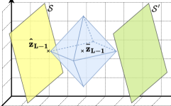
Figure 3: Geometry of the optimization problem (3). According to Proposition 4.4, the solution sets $\mathcal{S}$ (yellow) and $\mathcal{S}^{\prime}$ (green) for outputs $o$ and $o^{\prime}$, respectively, are shifted versions of another. The solution $\hat{z}_{L-1}$ is the point where the smallest $\ell_{1}$-diamond (blue) around $\bar{z}_{L-1}$ touches the solution set $\mathcal{S}$. In particular, the second and third components of $\hat{z}_{L-1}$, i.e., the ones corresponding to the $y$- and $z$-axis, coincide with the component of $\bar{z}_{L-1}$.

$$\begin{split}\hat{z}_{L-1}\in\operatorname*{arg\,min}_{z_{L-1}\in\mathbb{R}^{D_{L-1}}}\|z_{L-1}-\bar{z}_{L-1}\|_{1}\\ \text{subject to }o=G_{L}(z_{L-1})\enspace.\end{split}$$ (3)

This optimization problem is a modification of the basis pursuit algorithm (Chen, Donoho, and Saunders 2001); in particular, it has a similar interpretation: (3) returns solutions that are in the solution space $\mathcal{S}$ and are close to the average activation $\bar{z}_{L-1}$. The $\ell_{1}$-distance regularizes towards sparsity of $\hat{z}_{L-1}-\bar{z}_{L-1}$, i.e. towards many similar components of $\hat{z}_{L-1}$ and $\bar{z}_{L-1}$. We present a geometric illustration in Figure 3. In fact, exploiting the concept of sparsity is not new and has proven to be useful in theory and practice. For instance, Parhi and Nowak (2021) have shown that deep neural networks are implicitly learning sparse networks, Lederer (2022b) has derived statistical guarantees for deep networks under sparsity, sparsity is a ubiquitous concept in high-dimensional statistics (Lederer 2022a), and it has proven successful in compressed sensing as well (Eldar and Kutyniok 2012).

Finally, due to numerical inaccuracies of computations in high-dimensional linear systems, we allow for some slack $\varepsilon>0$ and simplify (3) to a modification of the basis pursuit denoising (Chen, Donoho, and Saunders 2001)

$$\begin{split}\hat{z}_{L-1}\in\operatorname*{arg\,min}_{z_{L-1}\in\mathbb{R}^{D_{L-1}}}\quad\|z_{L-1}-\bar{z}_{L-1}\|_{1}\\ \quad\text{subject to }\quad\|G_{L}(z_{L-1})-o\|_{2}\leq\varepsilon\enspace,\end{split}$$ (4)

which is equivalent to the well-known (modified) lasso (Tibshirani 1996) optimization problem, whose Lagrangian form is given by

$$\hat{z}_{L-1}\in\operatorname*{arg\,min}_{z_{L-1}\in\mathbb{R}^{D_{L-1}}}\|G_{L}(z_{L-1})-o\|_{2}^{2}+\lambda\|z_{L-1}-\bar{z}_{L-1}\|_{1},$$ (5)

where $\lambda>0$ is a parameter that depends on $\varepsilon$.

Re-examining the examples in Section 4.2, we see that our proposed optimization problem (5) now combines the underlying motivations of all three examples: The reconstruction loss guarantees to provide solutions that approximately solve the linear system (Example 4.1) and the regularization towards the average activation $\bar{z}_{L-1}$ biases the solutions towards reasonable activations (Example 4.2), which share a similar structure to $\bar{z}_{L-1}$ (Example 4.3). The rationale is that for an output $o^{-}$ that is not generated from $G$, we expect the estimated activations $\hat{z}$ necessary for approximately reconstructing $o^{-}$ using the model $G$ to be distinguishable from real activations of the model.

While our inversion scheme is closely related to the inversion methods from Section 3, we want to emphasize that FLIPAD enjoys several advantages summarized in the following theorem.

Theorem 4.5.

(Informal) Assume that $G_{L}$ is a 2D-convolution with kernel weights sampled from a continuous distribution ${\mathbf{k}}$. Then, (5) satisfies the following properties: (i) It is equivalent to a lasso optimization problem; (ii) It has a unique solution with probability $1$; (iii) Under certain moment assumption on ${\mathbf{k}}$ there exists some $S\in\mathbb{N}$ and constants $C_{0},C_{1}$ such that $\|\hat{z}-z\|_{2}\leq C_{0}/\sqrt{S}\|z-z_{S}\|_{1}+C_{1}$ if $\|z-\hat{z}\|_{0}\leq S$, where $z_{S}$ is the best $S$-term approximation of $z$.

Before providing a proof sketch, let us first examine the implications of Theorem 4.5: Property 1) allows us to use fast and computationally tractable lasso algorithms such as FISTA (Beck and Teboulle 2009), which enjoys finite-sample convergence guarantees. According to 2), it is not required to solve the optimization problem on multiple seeds, as in standard inversion techniques, see e.g. Section 3. Finally, 3) might be useful from a theoretical perspective but we want to highlight its limitations. The bound depends on $\|z-z_{S}\|_{1}$, which might be expected to be small in diverse problems in compressed sensing but it is not necessarily small for activations of a generative model. Finally, we provide a brief description of the proof. All details can be found in the supplement.

Proof.

(i) By a suitable zero-extension $0=-G_{L}(\bar{z})+G_{L}(\bar{z})$ within the $\ell_{2}$-norm in (5) and by using the linearity of $G_{L}$, we end up with a usual lasso optimization problem, see Section C.1. (ii) Lasso optimization problems have a unique solution if the columns of the design matrix are in general linear position (Tibshirani 2013). We show that this is the case for convolutions $G_{L}$ with probability $1$, see Section D. (iii) If $G_{L}$ satisfies the restricted isometry property (Candès 2008), then we can obtain bounds of the desired form for lasso optimization problems. We modify a result by Haupt et al. (2010) to prove this property for 2D-convolutions, see Section C.3. ∎

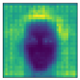
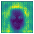
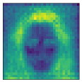
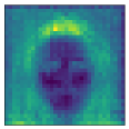
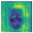
Figure 4: Cherry-picked channel dimension $c$ of the average reconstructed features according to (5) when $G$ is a DCGAN. The left-most figure shows the average activation $\bar{z}_{c}$ over channel $c$, the remaining figures show the average feature taken over DCGAN, real, WGAN-GP, LSGAN, and EBGAN samples, respectively.

5 Experiments

	CelebA					LSUN
	DCGAN	WGAN-GP	LSGAN	EBGAN		DCGAN	WGAN-GP	LSGAN	EBGAN
SM-F	64.81	50.18	53.57	95.78		69.94	52.96	56.30	74.58
$\text{SM-Inv}_{2}$	98.52	99.80	62.55	99.80		51.44	50.20	65.46	54.35
$\text{SM-Inv}_{\operatorname{inc}}$	51.23	50.16	52.64	78.46		50.61	50.35	51.61	52.12
RawPAD	94.95	59.12	99.53	99.54		67.14	52.36	98.22	93.96
DCTPAD	81.33	64.95	96.79	92.08		80.48	68.10	67.93	90.40
FLIPAD	99.34	99.40	98.94	99.68		97.75	97.73	98.19	99.38

Table 1: Single-model attribution accuracy averaged over all $G’\in\mathcal{G}$ over five runs. A more detailed report is provided in Table 7 in the Appendix. Note, due to their excessive computational load, we do not repeat the inversion methods multiple times.

	CelebA					LSUN
	DCGAN	WGAN-GP	LSGAN	EBGAN		DCGAN	WGANGP	LSGAN	EBGAN
RawPAD	95.77	61.49	97.48	74.35		61.82	51.65	92.71	90.46
DCTPAD	50.01	49.81	55.37	55.45		49.84	51.03	51.44	50.96
FLIPAD	99.31	97.88	69.75	99.76		98.04	97.52	88.84	89.79

Table 2: Average single-model attribution accuracy for the same model trained on different initialization seeds. Each score denotes the average accuracy over all $G’\in\mathcal{G}$ over five runs.

We demonstrate the effectiveness of the proposed methods—RawPAD, DCTPAD, and FLIPAD—in a range of extensive experiments. We begin with smaller generative models trained on CelebA and LSUN, which allow a fine-grained evaluation in various setups. We extend the experiments to modern large-scale diffusion models and style-based models, to medical image generators, and to tabular models.

5.1 Setup

Throughout all experiments, we train on $n_{\text{tr}}$ labeled samples $(x_{G},1)$ generated by $G$, and on $n_{\text{tr}}$ labeled negative samples $(x_{\text{neg}},-1)$ sampled either from the real set of images used to train $G$ or from another generative model $G^{\prime}$. The latter case is reasonable in settings, in which i) it is not entirely clear on what data $G$ was trained on (e.g. in Stable Diffusion) or ii) when the real data is not available at all (e.g. in medical applications). We repeat all experiments five times. To evaluate the performance, we measure the classification accuracy over $n_{\text{test}}$ samples from $G$ and $G’$, respectively, where $G’\in\mathcal{G}\backslash\{G\}$ for a set of generative models $\mathcal{G}$. We compare the proposed methods with fingerprinting (SM-F) and inversion ($\text{SM-Inv}_{2}$ and $\text{SM-Inv}_{\operatorname{inc}}$) methods, which we adapt to the single-model setting (see Section E). All experimental and architectural details as well as further empirical results, containing standard deviations to all experiments and visualizations, are deferred to Sections F and G in the Appendix.

5.2 Results

We begin by considering a set $\mathcal{G}$ of small generative models, namely DCGAN (Radford, Metz, and Chintala 2015), WGAN-GP (Gulrajani et al. 2017), LSGAN (Mao et al. 2017), EBGAN (Zhao, Mathieu, and LeCun 2016) trained on either the CelebA (Liu et al. 2015) or the LSUN bedroom (Yu et al. 2015) dataset.

Feature Extraction

As a first sanity check of the significance of the extracted features from (5), we present average features of images generated by different sources in Figure 4. While the average reconstructed features from images generated by the model are very close to its actual average activation, the other images exhibit fairly different features. We provide further examples and investigate the robustness with respect to the parameter $\lambda$ in Section G of the Appendix. These results provide qualitative evidence that the extracted features are distinguishable and detectable by an anomaly detector, which we demonstrate in the next paragraph.

Single-Model Attribution

We present the single-model attribution performance of each method in Table 1. First of all, we see that the adapted methods are very unstable, their accuracy ranges from $50$% to almost perfect attribution. Due to their inferior performance, yet high and restrictive computational costs of $\text{SM-Inv}_{2}$ and $\text{SM-Inv}_{\operatorname{inc}}$, we exclude them from the remaining experiments on those datasets. Even though RawPAD and DCTPAD are performing slightly better, their performance is not as consistent as FLIPAD’s, which achieves excellent results with an average attribution accuracy of over $97.5$% in all cases. In a second line of experiments, we evaluate the single-model attribution performance in a notably more difficult task: For a model $G$, we set $\mathcal{G}$ as the set of models with the exact same architecture and training data but initialized with a different seed. We present the results in Table 2 and observe a similar pattern as in the previous experiments. Since FLIPAD involves the knowledge of the exact weights of $G$, we argue that it enables reliable model attribution even in the case of these subtle model variations.

Single-Model Attribution on Perturbed Samples

To hinder model attribution, an adversary could perturb the generated samples. We investigate the attribution performance on perturbed samples in the immunized setting, i.e. we train the models on data that is modified by the same type of perturbation. For the sake of simplicity, we average the attribution accuracies over all models and present the results in Table 3. For blurred and cropped images we observe superior performance of FLIPAD over RawPAD and DCTPAD. However, in the case of JPEG compression and the presence of random noise, we can see a performance drop of FLIPAD. In contrast, those perturbations influence the performance of RawPAD only slightly. Table 11 demonstrates how the performance is improved by allowing a more liberal false negative rate (see Section F.1).

	CelebA									LSUN
	Blur		Crop		Noise		JPEG			Blur		Crop		Noise		JPEG
	1	3	60	55	0.05	0.1	90	80		1	3	60	55	0.05	0.1	90	80
RawPAD	88.71	87.86	88.69	89.33	84.09	80.36	87.05	86.45		77.73	76.65	76.24	75.76	73.47	69.86	75.68	74.87
DCTPAD	82.67	77.41	83.42	82.84	63.78	58.61	71.09	68.83		76.91	65.71	74.70	73.78	51.43	50.43	55.20	52.77
FLIPAD	99.36	98.34	98.25	98.27	76.06	68.80	83.46	81.36		98.13	97.21	94.64	89.96	66.58	53.17	72.83	67.70

Table 3: Single-model attribution accuracy with immunization averaged over all $G\in\mathcal{G},\;G’\in\mathcal{G}\backslash\{G\}$ over five runs. For blurring we consider kernel sizes of $1$ and $3$, for cropping we extract a center crop of $60\times 60$ and $55\times 55$ pixels followed by upsampling to $64\times 64$ pixels. For noise we use standard deviations of $0.05$ and $0.01$, for JPEG we use quality factors of 90 and 80.

	Stable Diffusion					Style-Based Models					Medical Image Models
	v1-4	v1-1	v1-1+	v2		real	StyleGAN-XL	StyleNAT	StyleSwin		WGAN-GP	C-DCGAN
SM-F	93.75	93.75	93.75	93.75		99.60	99.60	99.60	99.60		99.81	99.81
RawPAD	91.85	92.70	90.00	89.25		55.00	54.17	53.62	51.84		99.73	78.76
DCTPAD	95.45	95.55	49.40	48.90		99.93	99.93	99.54	99.85		99.73	71.49
FLIPAD	92.08	92.65	90.55	91.30		-	-	-	-		99.75	99.63

Table 4: Single-model attribution accuracy for Stable Diffusion v2-1, StyleGAN2, and DCGAN trained on BCDR. Each score denotes the average accuracy against $G’$ as indicated by the column name over five runs.

	TVAE	CTGAN	CopulaGAN
$\text{SM-Inv}_{2}$	88.02	95.74	94.45
RawPAD	90.61	96.60	94.93
FLIPAD	91.18	98.07	96.70

Table 5: Single-model attribution accuracy of KL-WGAN trained on Redwine against $G’$ as indicated by the column name averaged over five runs.

Stable Diffusion

In this experiment, we evaluate that FLIPAD is effective against the powerful text-to-image model Stable Diffusion (Rombach et al. 2022). Since multiple versions of Stable Diffusion have been released, an appropriate setting is to attribute images to a specific version. In particular, we consider Stable Diffusion v2-1 to be our model, while the set of other generators consists of v1-1, v1-1+ (similar to v1-1 but with a different autoencoder), v1-4, and v2. In contrast to previous experiments, we use images from v1-4 instead of real images for training, since it is not entirely clear on which data the model was trained. The results are provided in Table 4. All methods are able to distinguish between v2-1 and v1-4, which they are trained on. Given that v1-1 and v1-4 share the exact same autoencoder, this is less surprising. While DCTPAD fails to generalize to other generative models, the other approaches achieve high attribution accuracies above $90\%$ across all models.

Style-based Generative Models

In the next experiment, we analyze the single-model attribution of style-based generative models trained on FFHQ (Karras, Laine, and Aila 2019). Specifically, $\mathcal{G}$ consists of StyleGAN2 (Karras et al. 2021), StyleGAN-XL (Sauer, Schwarz, and Geiger 2022), StyleNAT (Walton et al. 2022), StyleSwin (Zhang et al. 2022), and of FFHQ images. We consider StyleGAN2 to be our model $G$. Note that the skip-connections in StyleGAN2 prohibit the application of FLIPAD. However, it is known that StyleGANs possess distinctive DCT artifacts (Frank et al. 2020), which DCTPAD benefits from, as demonstrated by the attribution accuracy in Table 4. The performance is on par with SM-F.

Generative Models for Medical Image Data

In contrast to the models in Section 5.2, generative models for medical images are facing very different challenges. Most importantly, medical data is typically much more scarce and the images are contextually different (Alyafi, Diaz, and Marti 2020; Varoquaux and Cheplygina 2022), which is why they requiring a separate treatment. We set $\mathcal{G}$ to consist of a DCGAN, a WGAN-GP, and a c-DCGAN (Szafranowska et al. 2022; Osuala et al. 2023) trained on the BCDR (Lopez et al. 2012), which contains $128\times 128$ breast mammography images. Since access to the original dataset is restricted, we train the models on samples from $\mathcal{G}$ and from WGAN-GP. We report the single-model attribution accuracies in Table 4 and observe that both, RawPAD and DCTPAD, are performing well on attributing samples from WGAN-GP but fail to generalize to C-DCGAN. Both, SM-F and FLIPAD, achieve close to perfect performance.

Generative Models for Tabular Data

Many model attribution methods are specifically tailored toward high-dimensional image data, such as SM-F, making use of well-studied image processing pipelines. However, to the best of our knowledge, there is not a single work conducting model attribution for tabular data, which we address in the following experiment. We set $\mathcal{G}$ to be the set consisting of KL-WGAN (Song and Ermon 2020), CTGAN, TVAE, and CopulaGAN (Xu et al. 2019) trained on the Redwine dataset (Cortez et al. 2009). Since the real dataset is small, we train the model attribution methods on samples from $\mathcal{G}$ and from TVAE. As displayed in Table 5, FLIPAD achieves the highest attribution performance for all $G’$.

Discussion

In summary, we conclude that, first, $\text{SM-Inv}_{2}$ and $\text{SM-Inv}_{\operatorname{inc}}$ perform well only in very few settings and their computational load restricts their practicality considerably. Second, SM-F achieves excellent performance for high-dimensional images but fails for low-dimensional images ($64\times 64$). Furthermore, its application is bound to the image domain. Third, RawPAD and DCTPAD are simple baselines that work decently in most settings but tend to generalize worse to the open-world setting. However, for the style-based generators, DCTPAD achieves excellent results, even for unseen generative models. Lastly, FLIPAD is capable to adapt to various settings and performs best, or only slight worse, than competing methods.

6 Conclusion

This work tackles a neglected but pressing problem: determining whether a sample was generated by a specific model or not. We associate this task, which we term single-model attribution, with anomaly detection—a connection that has not been drawn previously. While applying anomaly detection directly to the images performs reasonably well, the performance can be further enhanced by incorporating knowledge about the generative model. More precisely, we develop a novel feature-extraction technique based on final-layer inversion. Given an image, we reconstruct plausible activations before the final layer under the premise that it was generated by the model at hand. This reconstruction task can be reduced to a lasso optimization problem, which, unlike existing methods, can be optimized efficiently, globally, and uniquely. Beyond these beneficial theoretical properties, our approach is not bound to a specific domain and achieves excellent empirical results on a variety of different generative models, including GANs and diffusion models.

Appendix A Summary of the Related Work

We complement the summary provided in Section 3 with an overview given in Table 6.

	Method	Target	Setting
Fingerprinting	Marra et al. (2019a)	multi-model	closed-world
	Yu, Davis, and Fritz (2019)	multi-model	closed-world
	Xuan et al. (2019)	multi-model	closed-world
	Marra et al. (2019b)	multi-model	closed-world
	Frank et al. (2020)	multi-model	closed-world
Inversion	Albright and McCloskey (2019)	multi-model	closed-world
	Karras et al. (2020)	single-model	closed-world
	Zhang et al. (2021)	multi-model	closed-world
	Hirofumi et al. (2022)	both	both
Watermarking	Yu et al. (2021)	single-model	open-world
	Kim, Ren, and Yang (2021)	single-model	open-world
	Yu et al. (2022)	single-model	open-world
Ours		single-model	open-world

Table 6: Classification of the related work.

Appendix B Deep Semi-Supervised Anomaly Detection

In anomaly detection, we seek to identify samples that are most likely not generated by a given generative process. We call such samples out-of-distribution samples. But in contrast to classical binary classification procedures, anomaly detection methods strive for bounded decision areas for the in-distribution samples, while logistic regression for instance yields unbounded decision areas. For example, SVDD (Tax and Duin 2004) maps the data into a kernel-based feature space and finds the smallest hypersphere that encloses the majority of the data. Samples outside that hypersphere are then deemed as out-of-distribution samples. Recently, (Ruff et al. 2018) replaced the kernel-based feature space with a feature space modeled by a deep network, which was further extended to the semi-supervised setting in (Ruff et al. 2019). More specifically, given $n$ unlabeled samples $x_{1},\dots,x_{n}$, and $m$ labeled samples $(\tilde{x}_{1},\tilde{y}_{1}),\dots,(\tilde{x}_{m},\tilde{y}_{m})$, where $\tilde{y}=1$ denotes an inlier sample, and $\tilde{y}=-1$ denotes an outlier sample, Ruff et al. (2019) seek to find a feature transformation function $\phi$ parameterized by weights $\mathcal{W}=(W^{1},\dots W^{L})$. The corresponding optimization problem is defined as

$$\mathcal{W}^{\ast}\in\operatorname*{arg\,min}_{\mathcal{W}} \frac{1}{n+m}\sum_{i=1}^{n}\|\phi(x_{i};\mathcal{W})-c\|_{2}^{2}$$

$$+ \frac{\eta}{n+m}\sum_{j=1}^{n}\bigl{(}\|\phi(\tilde{x}_{j};\mathcal{W})-c\|_{2}^{2}\bigr{)}^{\tilde{y_{j}}}$$ (6)

$$+ \frac{\lambda}{2}\sum_{l=1}^{L}\|W^{l}\|_{F}^{2}\enspace,$$

where $\eta>0$ is a hyperparameter balancing the importance of the labeled samples, and $c$ is a point in the feature space representing the center of the hypersphere. Intuitively, out-of-distribution samples $x$ are mapped further away from $c$, resulting in a large $\ell_{2}$-distance $\|\phi(x;\mathcal{W}^{\ast})-c\|_{2}$ and AD is performed by fixing a threshold $\tau>0$ to classify

$$\hat{y}=\begin{cases}1\;&,\text{ if }\|\phi(x;\mathcal{W}^{\ast})-c\|_{2}\leq\tau\\ -1\;&,\text{ if }\|\phi(x;\mathcal{W}^{\ast})-c\|_{2}>\tau\end{cases}\enspace.$$ (7)

We explain how we tuned $\tau$ in Section F.1.

While DeepSAD has been applied to typical anomaly detection tasks, it has never been applied for attributing samples to a generative model. Moreover, in our setting described in Section 2, we assume to have only access to samples generated by $G$ and to real samples. Hence, DeepSAD reduces to a supervised anomaly detection method in this case.

Appendix C Recovery Guarantees for the Optimization Problem 5

In this section, we equip the proposed optimization problem (5) with theoretical recovery guarantees of the activation for random 2D-convolutions. First, we show in Section C.1 the equivalence of (5) to a standard lasso-problem. Hence, we can draw a connection to the theory of compressed sensing, which we briefly review in Section C.2. We show how 2D-convolutions originate from deleting rows and columns of a Toeplitz matrix in Section C.3, which motivates a proof for the restricted isometry property for 2D-convolutions. Finally, we generalize the recovery bounds for the classical lasso to our modified lasso problem in Section C.4.

C.1 (5) is equivalent to a Lasso-Problem

We can rewrite (5) as follows:

$$\hat{z}_{L-1} =\operatorname*{arg\,min}_{z_{L-1}\in\mathbb{R}^{D_{L-1}}}\|G_{L}(z_{L-1})-o\|_{2}^{2}+\lambda\|z_{L-1}-\bar{z}\|_{1}$$

$$=\operatorname*{arg\,min}_{z_{L-1}\in\mathbb{R}^{D_{L-1}}}\|G_{L}(z_{L-1})-G_{L}(\bar{z})+G_{L}(\bar{z})-o\|_{2}^{2}$$

$$\hskip 56.9055pt+\lambda\|z_{L-1}-\bar{z}\|_{1}$$

$$=\operatorname*{arg\,min}_{z_{L-1}\in\mathbb{R}^{D_{L-1}}}\|G_{L}(z_{L-1}-\bar{z})-(o-G_{L}(\bar{z}))\|_{2}^{2}$$

$$\hskip 56.9055pt+\lambda\|z_{L-1}-\bar{z}\|_{1}\enspace.$$

Furthermore, since

$$\min_{z_{L-1}\in\mathbb{R}^{D_{L-1}}}\|G_{L}(z_{L-1}-\bar{z}_{L-1})-o^{\prime}\|_{2}^{2}+\lambda\|z_{L-1}-\bar{z}_{L-1}\|_{1}$$

$$= \min_{z_{L-1}\in\mathbb{R}^{D_{L-1}}}\|G_{L}(z_{L-1})-o^{\prime}\|_{2}^{2}+\lambda\|z_{L-1}\|_{1}\enspace,$$

for $o^{\prime}:=o-G_{L}(\bar{z})$, we can recover $\hat{z}_{L-1}=\hat{z}_{L-1}^{\prime}+\bar{z}_{L-1}$, where

$$\hat{z}_{L-1}^{\prime}=\operatorname*{arg\,min}_{z_{L-1}\in\mathbb{R}^{D_{L-1}}}\|G_{L}(z_{L-1})-o^{\prime}\|_{2}^{2}+\lambda\|z_{L-1}\|_{1}\enspace.$$ (8)

Hence, to solve (5), we can solve (8) using standard lasso-algorithms such as FISTA (Beck and Teboulle 2009). Additionally, note that the optimization problem is convex and satisfies finite-sample convergence guarantees, see Beck and Teboulle (2009).

C.2 Background on Compressed Sensing

Having observed an output $o\in\mathbb{R}^{D_{\operatorname{out}}}$, the goal of compressed sensing is the recovery of a high-dimensional but structured signal $z^{\ast}\in\mathbb{R}^{D_{\operatorname{in}}}$ with $D_{\operatorname{in}}>>D_{\operatorname{out}}$ that has produced $o=\Phi(z^{\ast})$ for some transformation $\Phi:\mathbb{R}^{D_{\operatorname{in}}}\rightarrow\mathbb{R}^{D_{\operatorname{out}}}$. In its simplest form, we define $\Phi$ as a linear function that characterizes an underdetermined linear system

$$o=Gz^{\ast}$$

where $G\in\mathbb{R}^{D_{\operatorname{out}}\times D_{\operatorname{in}}}$ is the defining matrix of $\Phi$. $G$ is usually referred to as the measurement matrix. As stated in Proposition 4.4, there usually exists a vector space of solutions $\{z\in\mathbb{R}^{D_{\operatorname{in}}}|o=Gz\}$, and hence, signal recovery seems impossible. However, under certain assumptions on the true (but unknown) signal $z^{\ast}$ and measurement matrix $G$, we can derive algorithms that are guaranteed to recover $z^{\ast}$, which is the subject of compressed sensing. In this section, we review some results from compressed sensing for sparse signals along the lines of the survey paper by Eldar and Kutyniok (2012).

One fundamental recovery algorithm for sparse signals is the basis pursuit denoising (Chen, Donoho, and Saunders 2001)

$$\min_{z}\|z\|_{1}\;\text{subject to}\;\|G(z)-o\|_{2}\leq\varepsilon\enspace$$ (9)

for some noise level $\varepsilon>0$. Next, we define one set of assumptions on $z^{\ast}$ and $G$—namely sparsity of $z^{\ast}$ and the restricted isometry property of $G$—that allow the recovery of $z^{\ast}$ using (9).

Definition C.1.

For $S\in\mathbb{N}$, we call a vector $z\in\mathbb{R}^{D_{\operatorname{in}}}$ $S$-sparse, if

$$\|z\|_{0}:=\#\{j\in\{1,\dots,D_{\operatorname{in}}\}:z_{j}\neq 0\}\leq S\enspace.$$

We denote the set of all $S$-sparse vectors by $\Sigma_{S}\subset\mathbb{R}^{D_{\operatorname{in}}}$.

Definition C.2.

Let $G$ be a $D_{\operatorname{out}}\times D_{\operatorname{in}}$ matrix. We say $G$ has the restricted isometry property of order $S\in\mathbb{N}$, if there exists a $\delta_{S}\in(0,1)$ such that

$$(1-\delta_{S})\|z\|_{2}^{2}\leq\|Gz\|_{2}^{2}\leq(1+\delta_{S})\|z\|_{2}^{2}\enspace\forall z\in\Sigma_{S}\enspace.$$ (10)

In that case, we say that $G$ is $(S,\delta_{S})$-RIP.

To provide some intuition to that definition, note that $G$ is $(S,\delta_{S})$-RIP if

$$\|Gz\|_{2}^{2}=z^{\top}G^{\top}Gz\approx\|z\|_{2}^{2}=z^{\top}z\enspace\forall z\in\Sigma_{S}\enspace,$$

where the approximation is due to the bounds in (10). Hence, the RIP is, loosely speaking, related to the condition $z^{\top}G^{\top}Gz\approx z^{\top}z$ for $S$-sparse vectors $z$, i.e. $G$ behaves like an orthogonal matrix on vectors $z\in\Sigma_{S}$. In fact, the restricted isometry property can be interpreted as a generalized relaxation of orthogonality for non-square matrices.

Lastly, let us define $z_{S}$ as the best $S$-term approximation of $z^{\ast}$, i.e.

$$z_{S}=\operatorname*{arg\,min}_{z\in\Sigma_{S}}\|z^{\ast}-z\|_{1}\enspace.$$ (11)

Theorem C.3 (Noisy Recovery (Candès 2008)).

Assume that $G$ is $(2S,\delta_{2S})$-RIP with $\delta_{2S}<\sqrt{2}-1$ and let $\hat{z}$ be the solution to (9) with a noise-level $\|\varepsilon\|_{2}\leq E$. Then, there exist constants $C_{0},C_{1}$ such that

$$\|\hat{z}-z^{\ast}\|_{2}\leq\frac{C_{0}}{\sqrt{S}}\|z^{\ast}-z_{S}\|_{1}+C_{1}E\enspace.$$

This fundamental theorem allows deriving theoretical recovery bounds for sparse signals under the RIP-assumption on $G$. Unfortunately, the combinatorial nature of the RIP makes it difficult to certify. In fact, it has been shown that certifying RIP is NP-hard (Bandeira et al. 2013). However, it can be shown that random matrices drawn from a distribution satisfying a certain concentration inequality are RIP with high probability (Baraniuk et al. 2008). Those random matrices include, for instance, the set of Gaussian random matrices, which could be used to model random fully-connected layers.

In the remainder of Section C we will deal with the derivation of the RIP for random 2D-convolutions (Section C.3) and a modified version of Theorem C.3 for the proposed optimization problem (5) (Corollary C.8 and Section C.4).

C.3 Recovery Guarantees for 2D-Convolutions

To the best of our knowledge, there exist RIP-results for random convolutions, however, they are restricted to unsuited matrix distributions, such as Rademacher entries (Krahmer, Mendelson, and Rauhut 2013), and/or do not generalize to 2D-convolutions in their full generality (Haupt et al. 2010), including convolutions with multiple channels, padding, stride, and dilation. In this Section, we prove that randomly-generated 2D-convolutions indeed obey the restricted isometry property with high probability, which allows the application of recovery guarantees as provided by Theorem C.3. We begin by viewing 2D-convolutions as Toeplitz matrices with deleted rows and columns. In fact, this motivates a proof strategy for the RIP of 2D-convolutions by recycling prior results (Haupt et al. 2010).

Definition C.4.

Let $G\in\mathbb{R}^{D_{\operatorname{out}}\times D_{\operatorname{in}}}$ be a matrix given by

$$G:=\begin{pmatrix}g_{0}&g_{-1}&g_{-2}&\dots&\dots&g_{-(D_{\operatorname{in}}-1)}\\ g_{1}&g_{0}&g_{-1}&\ddots&&\vdots\\ g_{2}&g_{1}&\ddots&\ddots&\ddots&\vdots\\ \vdots&\ddots&\ddots&\ddots&g_{-1}&g_{-2}\\ \vdots&&\ddots&g_{1}&g_{0}&g_{-1}\\ g_{(D_{\operatorname{out}}-1)}&\dots&\dots&g_{2}&g_{1}&g_{0}\\ \end{pmatrix}\enspace.$$

Then, we call $G$ the Toeplitz matrix generated by the sequence $\{g_{i}\}_{i\in I}$ for $I:=\{-(D_{\operatorname{in}}-1),\dots,0,\dots,D_{\operatorname{out}}-1\}$.

We begin by illustrating the relationship between Toeplitz matrices and standard 2D-convolutions along the example depicted in Figure 5. Algorithmically, we can construct the matrix $G$ by performing the following steps. First, we begin with constructing the Toeplitz matrix $T(k)$ generated by the sequence

$$g_{0}=k_{0,0},\;g_{-1}=k_{0,1},\;g_{-4}=k_{1,0},\;g_{-5}=k_{1,1},$$

$$g_{j}=0\text{ for }j\not\in\{0,-1,-4,-5\}\enspace.$$

Secondly, we delete any row that corresponds to a non-conformal 2D-convolution, such as the convolution applied on the values $x_{0,3},\;x_{1,3},\;x_{1,0},\;x_{2,0}$, as illustrated in the last row in Figure 5. Similarly, we can implement strided convolutions by deleting rows of $T(k)$. Dilation is implemented by dilating $T(k)$, i.e. padding zeros in the sequence that generates $T(k)$ and multi-channel 2D-convolutions are implemented by simply stacking one-channel matrices $G_{\operatorname{channel}\,i}$ in a row-wise fashion. Padded 2D-convolutions can be implemented by either padding zeros to the input, see Figure 6, or by deleting the corresponding columns of $G$ without altering the input. In summary, we can construct a 2D-convolution by generating a Toeplitz matrix from the sequence of zero-padded kernel parameters, from which we delete $n_{r}$ rows and $n_{c}$ columns, where $n_{r}$ is given by the input dimensions and the stride, whereas $n_{c}$ is given by the padding.

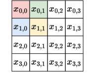
$\setcounter{MaxMatrixCols}{11}\begin{bmatrix}\lx@intercol\hfil\pagecolor{xred}k_{0,0}\hfil\lx@intercol&\lx@intercol\hfil\pagecolor{xgreen}k_{0,1}\hfil\lx@intercol&0&0&\lx@intercol\hfil\pagecolor{xblue}k_{1,0}\hfil\lx@intercol&\lx@intercol\hfil\pagecolor{xyellow}k_{1,1}\hfil\lx@intercol&0&0&0&0&\cdots\\ 0&k_{0,0}&k_{0,1}&0&0&k_{1,0}&k_{1,1}&0&0&0&\cdots\\ 0&0&k_{0,0}&k_{0,1}&0&0&k_{1,0}&k_{1,1}&0&0&\cdots\\ 0&0&0&0&k_{0,0}&k_{0,1}&0&0&k_{1,0}&k_{1,1}&\cdots\\ \vdots&\vdots&\vdots&\vdots&\vdots&\vdots&\vdots&\vdots&\vdots&\vdots&\ddots\\ \end{bmatrix}\begin{bmatrix}\lx@intercol\hfil\pagecolor{xred}x_{0,0}\hfil\lx@intercol\\ \lx@intercol\hfil\pagecolor{xgreen}x_{0,1}\hfil\lx@intercol\\ x_{0,2}\\ x_{0,3}\\ \lx@intercol\hfil\pagecolor{xblue}x_{1,0}\hfil\lx@intercol\\ \lx@intercol\hfil\pagecolor{xyellow}x_{1,1}\hfil\lx@intercol\\ x_{1,2}\\ x_{1,3}\\ \vdots\\ \end{bmatrix}$

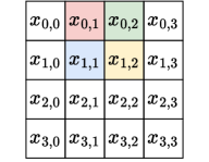
$\setcounter{MaxMatrixCols}{11}\begin{bmatrix}k_{0,0}&k_{0,1}&0&0&k_{1,0}&k_{1,1}&0&0&0&0&\cdots\\ 0&\lx@intercol\hfil\pagecolor{xred}k_{0,0}\hfil\lx@intercol&\lx@intercol\hfil\pagecolor{xgreen}k_{0,1}\hfil\lx@intercol&0&0&\lx@intercol\hfil\pagecolor{xblue}k_{1,0}\hfil\lx@intercol&\lx@intercol\hfil\pagecolor{xyellow}k_{1,1}\hfil\lx@intercol&0&0&0&\cdots\\ 0&0&k_{0,0}&k_{0,1}&0&0&k_{1,0}&k_{1,1}&0&0&\cdots\\ 0&0&0&0&k_{0,0}&k_{0,1}&0&0&k_{1,0}&k_{1,1}&\cdots\\ \vdots&\vdots&\vdots&\vdots&\vdots&\vdots&\vdots&\vdots&\vdots&\vdots&\ddots\\ \end{bmatrix}\begin{bmatrix}x_{0,0}\\ \lx@intercol\hfil\pagecolor{xred}x_{0,1}\hfil\lx@intercol\\ \lx@intercol\hfil\pagecolor{xgreen}x_{0,2}\hfil\lx@intercol\\ x_{0,3}\\ x_{1,0}\\ \lx@intercol\hfil\pagecolor{xblue}x_{1,1}\hfil\lx@intercol\\ \lx@intercol\hfil\pagecolor{xyellow}x_{1,2}\hfil\lx@intercol\\ x_{1,3}\\ \vdots\\ \end{bmatrix}$

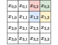
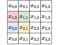
$\setcounter{MaxMatrixCols}{11}\begin{bmatrix}k_{0,0}&k_{0,1}&0&0&k_{1,0}&k_{1,1}&0&0&0&0&\cdots\\ 0&k_{0,0}&k_{0,1}&0&0&k_{1,0}&k_{1,1}&0&0&0&\cdots\\ 0&0&\lx@intercol\hfil\pagecolor{xred}k_{0,0}\hfil\lx@intercol&\lx@intercol\hfil\pagecolor{xgreen}k_{0,1}\hfil\lx@intercol&0&0&\lx@intercol\hfil\pagecolor{xblue}k_{1,0}\hfil\lx@intercol&\lx@intercol\hfil\pagecolor{xyellow}k_{1,1}\hfil\lx@intercol&0&0&\cdots\\ 0&0&0&0&k_{0,0}&k_{0,1}&0&0&k_{1,0}&k_{1,1}&\cdots\\ \vdots&\vdots&\vdots&\vdots&\vdots&\vdots&\vdots&\vdots&\vdots&\vdots&\ddots\\ \end{bmatrix}\begin{bmatrix}x_{0,0}\\ x_{0,1}\\ \lx@intercol\hfil\pagecolor{xred}x_{0,2}\hfil\lx@intercol\\ \lx@intercol\hfil\pagecolor{xgreen}x_{0,3}\hfil\lx@intercol\\ x_{1,0}\\ x_{1,1}\\ \lx@intercol\hfil\pagecolor{xblue}x_{1,2}\hfil\lx@intercol\\ \lx@intercol\hfil\pagecolor{xyellow}x_{1,3}\hfil\lx@intercol\\ \vdots\\ \end{bmatrix}$

$\setcounter{MaxMatrixCols}{11}\begin{bmatrix}k_{0,0}&k_{0,1}&0&0&k_{1,0}&k_{1,1}&0&0&0&0&\cdots\\ 0&k_{0,0}&k_{0,1}&0&0&k_{1,0}&k_{1,1}&0&0&0&\cdots\\ 0&0&k_{0,0}&k_{0,1}&0&0&k_{1,0}&k_{1,1}&0&0&\cdots\\ 0&0&0&0&\lx@intercol\hfil\pagecolor{xred}k_{0,0}\hfil\lx@intercol&\lx@intercol\hfil\pagecolor{xgreen}k_{0,1}\hfil\lx@intercol&0&0&\lx@intercol\hfil\pagecolor{xblue}k_{1,0}\hfil\lx@intercol&\lx@intercol\hfil\pagecolor{xyellow}k_{1,1}\hfil\lx@intercol&\cdots\\ \vdots&\vdots&\vdots&\vdots&\vdots&\vdots&\vdots&\vdots&\vdots&\vdots&\ddots\\ \end{bmatrix}\begin{bmatrix}\vdots\\ \lx@intercol\hfil\pagecolor{xred}x_{1,0}\hfil\lx@intercol\\ \lx@intercol\hfil\pagecolor{xgreen}x_{1,1}\hfil\lx@intercol\\ x_{1,2}\\ x_{1,3}\\ \lx@intercol\hfil\pagecolor{xblue}x_{2,0}\hfil\lx@intercol\\ \lx@intercol\hfil\pagecolor{xyellow}x_{2,1}\hfil\lx@intercol\\ x_{2,2}\\ x_{2,3}\\ \vdots\\ \end{bmatrix}$

Figure 5: Convolutional arithmetic as matrix multiplication. Each row shows one convolutional operation. Left: Conventional illustration of a 2D-convolution. Right: 2D-convolution as matrix multiplication $G\cdot x$.

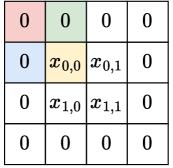
$\begin{bmatrix}\lx@intercol\hfil\pagecolor{xred}k_{0,0}\hfil\lx@intercol&\lx@intercol\hfil\pagecolor{xgreen}k_{0,1}\hfil\lx@intercol&0&0&\lx@intercol\hfil\pagecolor{xblue}k_{1,0}\hfil\lx@intercol&\lx@intercol\hfil\pagecolor{xyellow}k_{1,1}\hfil\lx@intercol&0&0&\cdots\\ 0&k_{0,0}&k_{0,1}&0&0&k_{1,0}&k_{1,1}&0&\cdots\\ 0&0&k_{0,0}&k_{0,1}&0&0&k_{1,0}&k_{1,1}&\cdots\\ \vdots&\vdots&\vdots&\vdots&\vdots&\vdots&\vdots&\vdots&\ddots\\ \end{bmatrix}\begin{bmatrix}\lx@intercol\hfil\pagecolor{xred}0\hfil\lx@intercol\\ \lx@intercol\hfil\pagecolor{xgreen}0\hfil\lx@intercol\\ 0\\ 0\\ \lx@intercol\hfil\pagecolor{xblue}0\hfil\lx@intercol\\ \lx@intercol\hfil\pagecolor{xyellow}x_{0,0}\hfil\lx@intercol\\ x_{0,1}\\ 0\\ \vdots\\ \end{bmatrix}$

Figure 6: Padded convolutional arithmetic as matrix multiplication. Left: Conventional illustration of a padded 2D-convolution. Right: 2D-convolution as matrix multiplication $G\cdot x$.

Those relationships motivate how we approach the proof for RIP for 2D-convolutions. First, we recycle a result by (Haupt et al. 2010) and generalize the restricted isometry property for Toeplitz matrices generated by sequences $\{g_{i}\}_{i=1}^{p}$ containing zeros (Theorem C.5). Secondly, we show that deleting rows and columns of the Toeplitz matrix retain the RIP to some extent (Lemma C.6 and Lemma C.7). Combining both ideas provides the RIP, and therefore a recovery bound, for random 2D-convolutions with multiple channels, padding, stride, and dilation (Corollary C.8).

Theorem C.5.

Let $\{g_{i}\}_{i=1}^{p}$ be a sequence of length $p=p_{0}+p_{r}$ such that

• $g_{i}=0$ for $i\in\mathcal{O}$ and

• $g_{i}\sim{\mathbf{g}}_{i}$, where ${\mathbf{g}}_{i}$ are i.i.d. zero-mean random variables with variance $\mathbb{E}({\mathbf{g}}_{i}^{2})=1/p_{r}$ and $|{\mathbf{g}}_{i}|\leq\sqrt{c/p_{r}}$ for some $c\geq 1$ and $i\not\in\mathcal{O}$,

where $\mathcal{O}\subset\{1,\dots,p\}$ with cardinality $|\mathcal{O}|=p_{0}$. Furthermore, let $G$ be the Toeplitz matrix generated by the sequence $\{g_{i}\}_{i=1}^{p}$. Then, for any $\delta_{S}\in(0,1)$ there exist constants $c_{1},c_{2}$, such that for any sparsity level $S\leq c_{2}\sqrt{p_{r}/\log(D_{\operatorname{in}})}$ it holds with probability at least $1-\exp(-c_{1}p_{r}/S^{2})$ that $G$ is $(S,\delta_{S})$-RIP.

This result is very similar to Theorem 6 by Haupt et al. (2010). In fact, the difference here is that we pad the sequence that generates the Toeplitz matrix by zero values $\{g_{i}\}_{i\in\mathcal{O}}$. To prove this modified version, we note that we can apply Lemma 6 and Lemma 7 by Haupt et al. (2010) for the sequence of zero-padded random variables $\{g_{i}\}_{i=1}^{p}$ as well. Besides that, we can perform the exact same steps as in the proof of Theorem 6 by Haupt et al. (2010), which is why we leave out the proof.

We want to highlight that the sparsity level $S$ and the probability for $G$ being $(S,\delta_{S})$-RIP both scale with $p_{r}$, which is essentially determined by the number of kernels and the kernel size of the 2D-convolution.

Lemma C.6.

Let $G\in\mathbb{R}^{D_{\operatorname{out}}\times D_{\operatorname{in}}}$ be $(S,\delta_{S})$-RIP and let $G_{:,-j}\in\mathbb{R}^{D_{\operatorname{out}}\times(D_{\operatorname{in}}-1)}$ be the matrix resulting from deleting the $j$th column from $G$. Then it follows that $G_{:,-j}$ is $(S-1,\delta_{S})$-RIP.

Proof.

Let $z^{\prime}\in\mathbb{R}^{D_{\operatorname{in}}-1}$ be a $S-1$-sparse vector and consider its zero-padded version $z\in\mathbb{R}^{D_{\operatorname{in}}}$ with marginals $z_{i}$ defined by

$$z_{i}:=\begin{cases}z^{\prime}_{i}\quad&\text{if }i<j\\ 0\quad&\text{if }i=j\\ z^{\prime_{i-1}}\quad&\text{if }i>j\end{cases}\enspace.$$

Note that $z$ is $S$-sparse and since $G$ is assumed to be $(S,\delta_{S})$-RIP it follows that

$$(1-\delta_{S})\|z\|_{2}^{2}\leq\|Gz\|_{2}^{2}\leq(1+\delta_{S})\|z\|_{2}^{2}\enspace.$$

It holds that

$$\|Gz\|_{2}^{2}=\|G_{:,-j}z^{\prime}\|_{2}^{2}\enspace\text{and}\enspace\|z\|_{2}^{2}=\|z^{\prime}\|_{2}^{2}\enspace$$

and therefore

$$(1-\delta_{S})\|z^{\prime}\|_{2}^{2}\leq\|G_{:,-j}z^{\prime}\|_{2}^{2}\leq(1+\delta_{S})\|z^{\prime}\|_{2}^{2}\enspace,$$

which proves that $G_{:,-j}$ is $(S-1,\delta_{S})$-RIP. ∎

Lemma C.7.

Let $G\in\mathbb{R}^{D_{\operatorname{out}}\times D_{\operatorname{in}}}$ be $(S,\delta_{S})$-RIP and let $G_{-j,:}\in\mathbb{R}^{(D_{\operatorname{out}}-1)\times D_{\operatorname{in}}}$ be the matrix resulting from deleting the $j$th row from $G$. Then it follows that $G_{-j,:}$ is $(S,\delta_{S}^{\prime})$-RIP, where

$$\delta_{S}^{\prime}:=\delta_{S}+S\max_{i}G_{j,i}^{2}\enspace.$$

Proof.

Let $z\in\Sigma_{S}$. Since $G$ is assumed to be $(S,\delta_{S})$-RIP, it holds that

$$\|G_{-j,:}z\|_{2}^{2}\leq\|Gz\|_{2}^{2}\leq(1+\delta_{S})\|z\|_{2}^{2}\leq(1+\delta_{S}^{\prime})\|z\|_{2}^{2}\enspace,$$

where the first inequality follows from the positivity of the summands, the second inequality follows from (10), and the third inequality follows from $\delta_{S}\leq\delta_{S}^{\prime}$. Hence, it remains to prove the lower bound from (10):

$$\|G_{-j,:}z\|_{2}^{2} =\sum_{\begin{subarray}{c}i=1\\ i\neq j\end{subarray}}^{D_{\operatorname{out}}}\bigl{(}G_{i,:}^{\top}z\bigr{)}^{2}$$

$$=\biggl{(}\sum_{i=1}^{D_{\operatorname{out}}}\bigl{(}G_{i,:}^{\top}z\bigr{)}^{2}\biggr{)}-\bigl{(}G_{j,:}^{\top}z\bigr{)}^{2}$$

$$=\biggl{(}\sum_{i=1}^{D_{\operatorname{out}}}\bigl{(}G_{i,:}^{\top}z\bigr{)}^{2}\biggr{)}-\bigl{(}G_{j,\mathcal{S}}^{\top}z_{\mathcal{S}}\bigr{)}^{2}\enspace,$$

where $\mathcal{S}:=\{j:z_{j}\neq 0\}$ denotes the support of $z$. Finally, we can apply the Cauchy-Schwartz inequality to conclude that

$$\|G_{-j,:}z\|_{2}^{2}\geq(1-\delta_{S})\|z\|_{2}^{2}-\|G_{j,\mathcal{S}}\|_{2}^{2}\|z_{\mathcal{S}}\|_{2}^{2}=(1-\delta_{S}^{\prime})\|z\|_{2}^{2}\enspace$$

since $\|z\|_{2}^{2}=\|z_{\mathcal{S}}\|_{2}^{2}$. Hence, $G_{j,:}$ is $(S,\delta_{S}^{\prime})$-RIP. ∎

Gathering our results, we can derive the following probabilistic recovery bound.

Corollary C.8.

Let $G$ be a 2D-convolution resulting from $n_{r}$ row deletions with $n_{k}$ kernel parameters sampled from an i.i.d. zero-mean random variables ${\mathbf{k}}_{i}$ with $\mathbb{E}({\mathbf{k}}_{i}^{2})=1/n_{k}$ and $|{\mathbf{k}}_{i}|\leq\sqrt{c/n_{k}}$ for some $c\geq 1$. Then, there exists a $S\in\mathbb{N}$ and $C_{0},C_{1},C_{2}\geq 0$ such that if additionally $|{\mathbf{k}}_{i}|\leq\sqrt{C_{2}/n_{d}S}$ then it holds with high probability that

$$\|\hat{z}-z^{\ast}\|_{2}\leq\frac{C_{0}}{\sqrt{S}}\|z^{\ast}-z_{S}\|_{1}+C_{1}E\enspace,$$ (12)

where $E\geq\|\varepsilon\|_{2}$ is the noise-level.

Proof.

From Theorem C.5, it follows that there exists a $\delta_{S}<\sqrt{2}-1$ and a sparsity level $S$ such that the Toeplitz matrix $T(G)$ corresponding to $G$ is $(\delta_{S},S)$-RIP with high probability. Furthermore, let us define $C_{2}:=\sqrt{2}-1-\delta_{S}$. By iteratively deleting $n_{d}$ rows from on $T(G)$, we end up with $G$, which is—according to Lemma C.6—$(\delta_{S}^{\prime},S)$-RIP with

$$\delta_{S}^{\prime}=\delta_{S}+n_{d}S\max_{i}k_{i}\leq\delta_{S}+n_{d}S\frac{C_{2}}{n_{d}S}=\delta_{S}+C_{2}=\sqrt{2}-1\enspace.$$

Hence, we can apply Theorem C.3 to conclude that there exist constants $C_{0},C_{1}$ such that

$$\|\hat{z}-z^{\ast}\|_{2}\leq\frac{C_{0}}{\sqrt{S}}\|z^{\ast}-z_{S}\|_{1}+C_{1}E\enspace.$$

∎

Note that by iteratively applying Lemma C.6, we can derive a similar result for 2D-convolutions that employ zero-padding, which we leave out for the sake of simplicity.

C.4 Extending the Results to the Optimization Problem (5)

So far, we have only derived recovery guarantees for solutions of the optimization problem (9). Fortunately, as presented in (8) in the main paper, we can readily draw a connection between (9) and (5).

Definition C.9 ($(\bar{z},S)$-Similarity).

Let $z,\bar{z}\in\mathbb{R}^{D}$. We say that $z$ is $(\bar{z},S)$-similar, if $\|z-\bar{z}\|_{0}$ is $S$-sparse. We denote the set of all $(\bar{z},S)$-similar vectors by $\Sigma_{S}(\bar{z})$.

In the following, we switch back to the notation from Section 4 but leave out the layer index to emphasize the generality of this Section, i.e.

$$\hat{z} =\operatorname*{arg\,min}_{z\in\mathbb{R}^{D_{\operatorname{in}}}}\|Gz-o\|_{2}^{2}+\lambda\|z-\bar{z}\|_{1}\enspace,$$

$$\hat{z}^{\prime} =\operatorname*{arg\,min}_{z\in\mathbb{R}^{D_{\operatorname{in}}}}\|Gz-o^{\prime}\|_{2}^{2}+\lambda\|z\|_{1}\enspace,$$

with $o^{\prime}=o-G\bar{z}=G(z^{\ast}-\bar{z})$. Since $z^{\ast}-\bar{z}$ is the input producing $o^{\prime}$, we define $z^{\ast\prime}=z^{\ast}-\bar{z}$. Then, we can readily extend sparse recovery results, such as Corollary C.8, to $(\bar{z},S)$-similar recovery results by applying a simple zero-extensions:

$$\|\hat{z}-z^{\ast}\|_{2}^{2} =\|\hat{z}-\bar{z}+\bar{z}-z^{\ast}\|_{2}^{2}=\|(\hat{z}-\bar{z})-(z^{\ast}-\bar{z})\|_{2}^{2}$$

$$=\|\hat{z}^{\prime}-z^{\ast\prime}\|_{2}^{2}\enspace.$$

The right-hand side can be upper-bounded by our sparse recovery bound (12) since, per definition, $(\bar{z},S)$-similarity of $z^{\ast}$ implies $S$-sparsity of $z^{\ast\prime}$.

Appendix D Uniqueness of the Solution of (5)

The optimization problem (5) can be reformulated as an equivalent lasso optimization problem (Section C.1), offering the advantage of leveraging efficient optimization algorithms like FISTA (Beck and Teboulle 2009), which are guaranteed to converge. In addition, we show in this section that the solution is also unique, i.e. FISTA converges to a unique solution. Therefore, there is no need to solve the optimization problem for different seeds, as seen in similar methods discussed in Section 3. We prove the uniqueness by applying techniques from Tibshirani (2013).
In the following, we assume that $D_{\operatorname{in}}>D_{\operatorname{out}}$.

Definition D.1.

Let $G\in\mathbb{R}^{D_{\operatorname{out}}\times D_{\operatorname{in}}}$. We say that $G$ has columns in general position if for any selection of columns $G_{i_{1}},\dots,G_{i_{D_{\operatorname{in}}}}$ of $G$ and any signs $\sigma_{1},\dots,\sigma_{i_{D_{\operatorname{in}}}}\in\{-1,1\}$ it holds

$$\operatorname{Aff}(\{\sigma_{1}G_{i_{1}},\dots,\sigma_{n}G_{i_{D_{\operatorname{in}}}}\})\cap\{\pm G_{i}:\;i\not\in\{i_{1},\dots,i_{D_{\operatorname{in}}}\}\}=\emptyset\enspace,$$

where $\operatorname{Aff}(S):=\{\sum_{n=1}^{N}\lambda_{n}s_{n}:\;\sum_{n=1}^{N}\lambda_{n}=1\}$ defines the affine hull of the set $S=\{s_{1},\dots,s_{N}\}$.

Lemma D.2 ((Tibshirani 2013)).

If the columns of $G\in\mathbb{R}^{D_{\operatorname{out}}\times D_{\operatorname{in}}}$ are in general position, then for any $\lambda>0,\,o\in\mathbb{R}^{D_{\operatorname{out}}}$ the lasso problem

$$\hat{z}=\operatorname*{arg\,min}_{z\in\mathbb{R}^{D_{\operatorname{in}}}}\|Gz-o\|_{2}^{2}+\lambda\|z\|_{1}$$

has a unique solution.

In the following, we prove that a $2D$-convolution has columns in general position.

Proposition D.3.

Let $G\in\mathbb{R}^{D_{\operatorname{out}}\times D_{\operatorname{in}}}$ be a 2D-convolution with kernel $k\in\mathbb{R}^{D_{k}}$ with pairwise different kernel values and $D_{k}\geq 2$. Then, there exist binary matrices $U_{j}\in\{0,1\}^{D_{\operatorname{out}}\times D_{\operatorname{in}}}$ for $j\in\{1,\dots,D_{\operatorname{in}}\}$ such that:

1. the $j$th column of $G$ can be written as $G_{j}=U_{j}\cdot k\in\mathbb{R}^{D_{\operatorname{out}}}$  ;

2. The supports of $U_{j}$,

   $$S_{j}:=\{(l,m)\in\{1,\dots,D_{\operatorname{out}}\}\times\{1,\dots,D_{\operatorname{in}}\}:\bigl{(}U_{j}\bigr{)}_{l,m}\neq 0\}$$

   are pairwise disjoint for all $j$.

Proof.

$G$ is a 2D-convolution, therefore, each column $G_{j}$ is a sparse vector with $l$th entry $(G_{j})_{l}\in\{0,k_{1},\dots,k_{D_{k}}\}$, i.e. it is either $0$ or one of the kernel values. Hence, we can define the $U_{j}$ by

$$(U_{j})_{l,m}=\begin{cases}1\enspace,\quad&\text{if }(G_{j})_{l}=k_{m}\\ 0\enspace,\quad&\text{otherwise }\end{cases}$$ (13)

for all $(l,m)\in\{1,\dots,D_{\operatorname{out}}\}\times\{1,\dots,D_{\operatorname{in}}\}$. Using that construction, we get

$$\bigl{(}U_{j}\cdot k\bigr{)}_{l} =(U_{j})_{l}\cdot k$$

$$=\begin{cases}k_{m}&\enspace,\text{if }(G_{j})_{l}=k_{m}\\ 0&\enspace,\text{otherwise}\end{cases}\enspace$$

$$=(G_{j})_{l}\enspace\text{ for all }l\in\{1,\dots,D_{\operatorname{out}}\}\enspace,$$

where $(U_{j})_{l}$ denotes the $l$th row of $U_{j}$. This proves the first claim, that is, $G_{j}=U_{j}\cdot k$. The second claim becomes immediate from our construction: Assume that there exist $j,j^{\prime}$ with $j\neq j^{\prime}$ but $S_{j}\cap S_{j^{\prime}}\neq\emptyset$. This means that there exists a $(l,m)$ such that $(U_{j})_{l,m}=(U_{j^{\prime}})_{l,m}$. According to (13), this means that $(G_{j})_{l}=k_{m}=(G_{j^{\prime}})_{l}$, which contradicts the Toeplitz-like structure of $G$, see Section C.3. Hence, $S_{j}$ and $S_{j\prime}$ must be disjoint. ∎

Theorem D.4.

Let $G\in\mathbb{R}^{D_{\operatorname{out}}\times D_{\operatorname{in}}}$ be a 2D-convolution with kernel values $k_{j}$ sampled from independent continuous random variables ${\mathbf{k}}_{j}$. Then, $G$ has columns in general position with probability $1$.

Before proving Theorem D.4, let us provide a basic result from linear algebra.

Lemma D.5.

Let $G_{1},\dots,G_{n+1}\in\mathbb{R}^{D}$ for some $n,D\in\mathbb{N}$. Then it is

$$G_{n+1}\in\operatorname{Aff}(\{G_{1},\dots,G_{n}\})$$

$$\Leftrightarrow\quad G_{n+1}-G_{n}\in\operatorname{span}(G_{1}-G_{n},\dots,G_{n-1}-G_{n})\enspace,$$

where $\operatorname{span}$ denotes the linear span.

Proof.

Let $G_{n+1}-G_{n}\in\operatorname{span}(G_{1}-G_{n},\dots,G_{n-1}-G_{n})$. Therefore, there exist $\lambda_{1},\dots,\lambda_{n-1}\in\mathbb{R}$ such that

$$G_{n+1}-G_{n} =\sum_{j=1}^{n-1}\lambda_{j}(G_{j}-G_{n})$$

$$\Leftrightarrow G_{n+1} =\sum_{j=1}^{n-1}\lambda_{j}G_{j}-\sum_{j=1}^{n-1}\lambda_{j}G_{n}+G_{n}$$

$$\Leftrightarrow G_{n+1} =\sum_{j=1}^{n-1}\lambda_{j}G_{j}+\biggl{(}1-\sum_{j=1}^{n-1}\lambda_{j}\biggr{)}G_{n}\enspace.$$

The above coefficients of $G_{j}$ satisfy

$$\sum_{j=1}^{n-1}\lambda_{j}+\biggl{(}1-\sum_{j=1}^{n-1}\lambda_{j}\biggr{)}=1\enspace.$$

Therefore, we have shown that there exist coefficients $\lambda_{j}^{\prime}$ such that $G_{n+1}=\sum_{j=1}^{n}\lambda_{j}^{\prime}G_{j}$, that is, $G_{n+1}\in\operatorname{Aff}(\{G_{1},\dots,G_{n}\}$.
Conversely, let $G_{n+1}\in\operatorname{Aff}(\{G_{1},\dots,G_{n}\}$. Then, there exist $\lambda_{1},\dots,\lambda_{n}\in\mathbb{R}$ with $\sum_{j=1}^{n}\lambda_{j}=1$ such that

$$G_{n+1} =\sum_{j=1}^{n}\lambda_{j}G_{j}$$

$$\Leftrightarrow\quad G_{n+1}-G_{n} =\sum_{j=1}^{n}\lambda_{j}G_{j}-G_{n}$$

$$=\sum_{j=1}^{n}\lambda_{j}G_{j}-\sum_{j=1}^{n}\lambda_{j}G_{n}$$

$$=\sum_{j=1}^{n}\lambda_{j}(G_{j}-G_{n})\enspace,$$

which proves that $G_{n+1}-G_{n}\in\operatorname{span}(G_{1}-G_{n},\dots,G_{n-1}-G_{n})$. ∎

Next, we provide the proof of Theorem D.4.

Proof.

Let $G_{i_{1}},\dots,G_{i_{D_{\operatorname{in}}}},G_{i_{D_{\operatorname{in}}+1}}$ be a collection of $D_{\operatorname{in}}+1$ columns of $G$. We show that $G_{i_{D_{\operatorname{in}}+1}}\in\operatorname{Aff}(\{G_{i_{1}},\dots,G_{i_{D_{\operatorname{in}}}}\})$ by proving that $G_{i_{D_{\operatorname{in}}+1}}-G_{i_{D_{\operatorname{in}}}}\in\operatorname{span}(G_{i_{1}}-G_{i_{D_{\operatorname{in}}}},\dots,G_{i_{D_{\operatorname{in}}-1}}-G_{i_{D_{\operatorname{in}}}})$ with probability $1$, see Lemma D.5. According to Proposition D.3, there exist binary matrices $U_{j}$ such that

$$G_{i_{D_{\operatorname{in}}+1}}-G_{i_{D_{\operatorname{in}}}}\in\operatorname{span}(G_{i_{1}}-G_{i_{D_{\operatorname{in}}}},$$

$$\quad\quad\dots,G_{i_{D_{\operatorname{in}}-1}}-G_{i_{D_{\operatorname{in}}}})$$

$$\Leftrightarrow \;(U_{i_{D_{\operatorname{in}}+1}}-U_{i_{D_{\operatorname{in}}}})\cdot k\in\operatorname{span}((U_{i_{1}}-U_{i_{D_{\operatorname{in}}}})\cdot k,$$

$$\quad\quad\dots,(U_{i_{D_{\operatorname{in}}-1}}-U_{i_{D_{\operatorname{in}}}})\cdot k)$$

$$\Leftrightarrow \;\exists(\lambda_{1},\dots,\lambda_{D_{\operatorname{in}}-1})\neq(0,\dots,0):$$

$$(U_{i_{D_{\operatorname{in}}}}-U_{i_{D_{\operatorname{in}}-1}})\cdot k=\sum_{j=1}^{D_{\operatorname{in}}-1}\lambda_{j}(U_{i_{j}}-U_{i_{D_{\operatorname{in}}}})\cdot k$$

$$\Leftrightarrow \;\exists(\lambda_{1},\dots,\lambda_{D_{\operatorname{in}}-1})\neq(0,\dots,0):$$

$$0=\biggl{(}\sum_{\begin{subarray}{c}j=1\\ j\neq D_{\operatorname{in}}\end{subarray}}^{D_{\operatorname{in}}+1}\lambda_{j}(U_{i_{j}}-U_{i_{D_{\operatorname{in}}}})\biggr{)}\cdot k,\enspace\text{ with }\lambda_{D_{\operatorname{in}}+1}:=-1$$

$$\Rightarrow \;k\in\operatorname{nul}\biggl{(}\sum_{\begin{subarray}{c}j=1\\ j\neq D_{\operatorname{in}}\end{subarray}}^{D_{\operatorname{in}}+1}\lambda_{j}(U_{i_{j}}-U_{i_{D_{\operatorname{in}}}})\biggr{)}\enspace$$ (14)

$$\text{ for the above choice of }\lambda_{1},\dots\lambda_{D_{\operatorname{in}}-1},\lambda_{D_{\operatorname{in}}+1}\enspace,$$

where $\operatorname{nul}(A)$ denotes the null-space of $A$. We show that (14) holds with probability $0$ by proving that the null-space has dimension less than $D_{k}$. By the rank-nullity theorem, this is equivalent to showing that

$$\operatorname{rank}(U)\geq 1\enspace\text{ for }U:=\sum_{\begin{subarray}{c}j=1\\ j\neq D_{\operatorname{in}}\end{subarray}}^{D_{\operatorname{in}}+1}\lambda_{j}(U_{i_{j}}-U_{i_{D_{\operatorname{in}}}})\enspace.$$

Since $U$ is a linear mapping, it is sufficient to show that there exists some $k\in\mathbb{R}$ such that $Uk\neq 0$.
Without loss of generality, let $\lambda_{1}\neq 0$. Then, since $U_{1}\neq 0$, we know that there exist some $l,m$ such that $(U_{1})_{l,m}=1$. Then, it holds for $k=e_{m}$, where $e_{m}$ is the $m$th euclidean unit vector, that

$$\bigl{(}Uk\bigr{)}_{l} =\biggl{(}\sum_{j=1}^{D_{\operatorname{in}}-1}\lambda_{j}U_{j}e_{m}-\sum_{j=1}^{D_{\operatorname{in}}-1}\lambda_{j}U_{D_{\operatorname{in}}}e_{m}\biggr{)}_{l}$$

$$=\biggl{(}\sum_{j=1}^{D_{\operatorname{in}}}\lambda_{j}U_{j}e_{m}\biggr{)}_{l}=\lambda_{1}\neq 0\enspace,$$

where $\lambda_{D_{\operatorname{in}}}:=-\sum_{j=1}^{D_{\operatorname{in}}}\lambda_{j}$. Note, the last equality follows by the fact that all $U_{j}$ have pairwise disjoint supports. Since the $l$th component of $Uk$ is not zero, we conclude that there exists some $k\in\mathbb{R}^{D_{k}}$ such that $Uk\neq 0$. Therefore, $\operatorname{rank}(U)\geq 1$, from which derive that $\operatorname{dim}(\operatorname{nul}(U))<D_{k}$, i.e. the null-space of $U$ has Lebesgue mass $0$.
In summary, if $G_{i_{D_{\operatorname{in}}+1}}\in\operatorname{Aff}(\{G_{i_{1}},\dots,G_{i_{D_{\operatorname{in}}}}\})$, then $k$ needs to be in a Lebesgue null-set, which has probability $0$ since ${\mathbf{k}}_{j}$ are assumed to be continuous random variables. We can repeat the same arguments independent of the sign of $G_{i_{D_{\operatorname{in}}+1}}$, the sign of $G_{i_{1}},\dots,G_{i_{D_{\operatorname{in}}}}$, for each $G_{i}$ with $i\not\in\{i_{1},\dots,i_{D_{\operatorname{in}}}\}$, and for any collection of $\{i_{1},\dots,i_{D_{\operatorname{in}}}\}$. By taking a union bound over all choices, we conclude that the columns of $G$ are in general position with probability $1$. ∎

Finally, plugging the pieces together, we prove the uniqueness of (5).

Corollary D.6.

Let $G\in\mathbb{R}^{D_{\operatorname{out}}\times D_{\operatorname{in}}}$ be a 2D-convolution with kernel values $k_{j}$ sampled from independent continuous random variables ${\mathbf{k}}_{j}$. Then, the optimization problem (5) has a unique solution with probability $1$.

Proof.

As shown in Section C.1, we can rewrite (5) to the equivalent lasso optimization problem (8). According to Theorem D.4, the columns of $G$ are in general linear position with probability $1$. Using Lemma D.2, we conclude that (5) has a unique solution with probability $1$. ∎

Appendix E Adapting Closed-World Attribution Methods to the Open-World Setting

While the method proposed in this work provides an efficient solution to the problem of single-model attribution in the open-world setting, it might not be suitable under all circumstances (e.g., if final-layer inversion is infeasible due to non-invertible ReLU-activations). Furthermore, if a particularly effective method exists in the closed-world setting, it might be beneficial to build upon this strong foundation. We, therefore, propose two adapted methods, SM (single-model)-Fingerprinting and SM-Inversion, which leverage the existing approaches to the open-world setting. Both return an anomaly score $s(x)$ that can be used to identify outliers by comparing it to a threshold $\tau$. All samples with an anomaly score greater than $\tau$ are classified as outliers.

SM-Fingerprinting

Marra et al. (2019a) propose to use the photo response non-uniformity (PRNU) to obtain noise residuals from images. The fingerprint $f_{G}$ is computed by averaging the residuals over a sufficient amount of images generated by $G$. Given an unknown image $x$, the anomaly score is defined as the negative inner product between $x$ and $f_{G}$, $s(x):=-\tilde{f}_{G}^{\top}\tilde{x}$, where $\tilde{f}_{G}$ and $\tilde{x}$ are the flattened and standardized versions of $\tilde{f}_{G}$ and $x$, respectively. In the following, we refer to this kind of SM-Fingerprinting as SM-F.

SM-Inversion

For inversion-based methods, the anomaly score is naturally given by the distance between the original image $x\in\mathbb{R}^{D}$ and its best reconstruction $G(\hat{z})$. It is defined as $s(x):=1/{D}\|x-G(\hat{z})\|$, where $\|\cdot\|$ is either the $\ell_{2}$-norm (Albright and McCloskey 2019) or a distance based on a pre-trained Inception-V3 (Szegedy et al. 2016) as proposed by Zhang et al. (2021). In the following, we refer to the two variants as $\text{SM-Inv}_{2}$ and $\text{SM-Inv}_{\operatorname{inc}}$. The reconstruction seed $\hat{z}$ is found by performing multiple gradient-based reconstruction attempts, each initialized on a different seed, and selecting the solution resulting in the smallest reconstruction distance.

Appendix F Experimental Details

F.1 Thresholding Method

We select the threshold $\tau$ in (7) by fixing a false negative rate $\operatorname{fnr}$ and set $\tau$ as the $(1-\operatorname{fnr})$-quantile of $\{s(x)\}_{x_{i}\in\mathcal{X}_{\operatorname{val}}}$, where $s(x)$ is the anomaly score function and $\mathcal{X}_{\operatorname{val}}$ is a validation set consisting of $n_{\text{val}}$ inlier samples (i.e., generated by $G$). We specify $n_{\text{val}}$ for each experiment is the following sections. In all of our experiments, we set $\operatorname{fnr}=0.005$ or $\operatorname{fnr}=0.05$ in the case of the Stable Diffusion experiments. In the latter, we decide to set a higher $\operatorname{fnr}$ due to the smaller validation set size.

F.2 Generative Models trained on CelebA and LSUN

In the following, we describe the generative models utilized in Section 5 in full detail. All models were optimized using Adam with a batch size of $128$, a learning rate of $0.0002$ and—if not stated differently—parameters $\beta_{1}=0.5,\,\beta_{2}=0.999$. The goal was not to train SOTA-models but rather to provide a diverse set of generative models as baselines for evaluating attribution performances in the setting described in Section 2. We visualize generated samples in Figure 7. All experiments on CelebA and LSUN utilize $n_{\text{tr}}=10\,000$ and $n_{\text{val}}=n_{\text{test}}=1\,000$ samples.

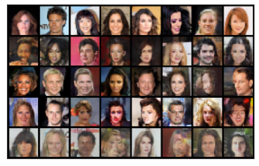
(a) CelebA

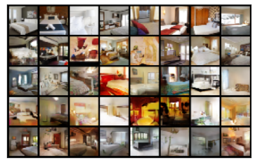
(b) LSUN

Figure 7: Examples of generated images. The first row represents real images, and each further row represents samples from DCGAN, WGAN-GP, LSGAN, EBGAN, respectively.

DCGAN

Our DCGAN Generator has $5$ layers, where the first 4 layers consist of a transposed convolution, followed by batchnorm and a ReLU-activation, and the last layer consists of a transposed convolution (without bias) and a $\operatorname{tanh}$-activation. The transposed convolutions in- and output-channel dimensions are $100\rightarrow 512\rightarrow 256\rightarrow 128\rightarrow 64\rightarrow 3$ and have a kernel size of $4$, stride of $2$, and a padding of $1$ (besides the first transposed convolution, which has a padding of $0$). The discriminator has $5$ layers, where the first layer is a convolution (without bias) followed by a leaky-ReLU-activation, the next $3$ are consist of a convolution, batchnorm, and leaky-ReLU-activation, and the last layer consists of a convolution and a final sigmoid-activation. We set the leaky-ReLU tuning parameter to $0.2$. The convolutions channel dimensions are $3\rightarrow 64\rightarrow 128\rightarrow 256\rightarrow 512\rightarrow 1$, and we employed a kernel of size $4$, stride of $2$, and a padding of $1$ in all but the last layer, which has a padding of $0$. We used soft-labels of $0.1$ and $0.9$ and trained the generator in each iteration for $50$ and $10$ epochs for CelebA and LSUN, respectively.

WGAN-GP

We utilized the same architecture for the generator as the one in DCGAN. The discriminator is similar to the one in DCGAN but uses layernorm instead of batchnorm and has no sigmoid-activation at the end. We trained the generator every $5$th iteration and utilized a gradient penalty of $\lambda=10$. In that case, we used $\beta_{1}=0.0$ and $\beta_{2}=0.9$ as Adam parameters and trained for $200$ and $10$ epochs for CelebA and LSUN, respectively.

LSGAN

The generator consists of a linear layer mapping from $100$ to $128\times 8\times 8$ dimensions, followed by 3 layers, each consisting of a nearest-neighbor upsampling ($\times 2$), a convolution, batchnorm, and a ReLU-activation. The final layer consists of a convolution, followed by a $\operatorname{tanh}$-activation. The convolution channel dimensions are $128\rightarrow 128\rightarrow 128\rightarrow 64\rightarrow 3$ and utilize a kernel of size $3$, stride of $1$, and a padding of $1$. The discriminator consists of $5$ layers discriminator blocks and a final linear layer. Each discriminator block contains a convolution, leaky-ReLU with parameter $0.2$, dropout with probability $0.25$, and batchnorm in all but the first layer. The convolution channel dimensions are $3\rightarrow 16\rightarrow 32\rightarrow 64\rightarrow 128\rightarrow 128$ and have a kernel of size $3$, stride of $2$, and padding of $1$. The final linear layer maps from $512$ to $1$ dimensions. We trained the generator every $5$th iteration for $100$ and $10$ epochs for CelebA and LSUN, respectively.

EBGAN

The architecture of the generator is similar to the one of the DCGAN generator. The discriminator uses an encoder-decoder architecture. The encoder employs convolutions (without bias) mapping from $3\rightarrow 64\rightarrow 128\rightarrow 256$ channel dimensions, each having a kernel of size $4$, stride of $2$, and padding of $1$. Between each convolution, we use batchnorm and a leaky-ReLU-activation with parameter $0.2$. The decoder has a similar structure but uses transposed convolutions instead of convolutions with channel dimensions $256\rightarrow 128\rightarrow 64\rightarrow 3$ and ReLUs instead of leaky-ReLUs. We set the pull-away parameter to $0.1$ and trained the generator every $5$th iteration for $100$ and $5$ epochs for CelebA and LSUN, respectively.

F.3 Stable Diffusion

We generate samples using the diffusers library which provides checkpoints for each version of Stable Diffusion. We use a subset of the COCO2014 annotations (Lin et al. 2014) as prompts and sample with default settings. All generated images have a resolution of $512\times 512$ pixels. We set $n_{\text{tr}}=2\,000,\;n_{\text{val}}=100,\;n_{\text{test}}=200$.

F.4 Style-based Generators

Each style-based generative model comes with an official implementation, which offers pre-trained models on FFHQ for download. We used those implementations to generate $n_{\text{tr}}=10\,000,\;n_{\text{val}}=n_{\text{test}}=1\,000$ images of resolution $256\times 256$.

F.5 Medical Image Generators

We sampled from the pretrained models provided by the medigan library (Osuala et al. 2023). The model identifiers are 5, 6, and 12 for the DCGAN, WGAN-GP, and c-DCGAN, respectively. The resolution images have a resolution of $128\times 128$ pixels. We set $n_{\text{tr}}=10\,000,\;n_{\text{val}}=n_{\text{test}}=1\,000$.

F.6 Tabular Generators

The KL-WGAN was trained for $500$ epochs as specified in Song and Ermon (2020) using the official repository. CTGAN, TVAE, and Copula GAN were trained using the implementations and the default settings provided by the SDV library (Patki, Wedge, and Veeramachaneni 2016). We set $n_{\text{tr}}=100\,000$ and $n_{\text{val}}=n_{\text{test}}=10\,000$.

F.7 Hyperparameters of Attribution Methods

DeepSAD

DeepSAD uses the $\ell_{2}$-distance to the center $c$ as anomaly score, see (7). We propose $3$ variants of DeepSAD for the problem of single-model attribution:

1. RawPAD, i.e. DeepSAD trained on downsampled versions of the images. In the experiments involving the architectures from Section F.2, we downsample to $32\times 32$ images using nearest neighbors interpolation. In the Stable Diffusion experiments, we center-crop to $128\times 128$ images due to the large downsampling factor. In the style-based experiments, we downsample to $128\times 128$ using nearest neighbors interpolation. When the image is downsampled to $32\times 32$, we set $\phi$ as the 3-layer LeNet that was used on CIFAR-10 in Ruff et al. (2019), otherwise we use a 4-layer version of the LeNet-architecture. In the tabular experiments, we set $\phi$ to be a standard feed-forward network with hidden dimensions $512\rightarrow 1024\rightarrow 1024\rightarrow 512\rightarrow 256\rightarrow 128$.

2. DCTPAD, i.e. DeepSAD on the downsampled DCT features of the images. We obtain those features by computing the 2-dimensional DCT on each channel, adding a small constant ${\epsilon}=1e^{-10}$ for numerical stability, and taking the $\operatorname{log}$. To avoid distorting the DCT-spectra, we reduce the image size by taking center-crops. We use the same architecture $\phi$ as in RawPAD.

3. FLIPAD, i.e. DeepSAD on activations result from the optimization problem (5). We solved the optimization problem using FISTA (Beck and Teboulle 2009) with the regularization parameter $\lambda$ set to $0.0005$ for the experiments involving the models from Section F.2, to $0.00001$ for the Stable Diffusion experiments, to $0.001$ for the medical image experiments, and to $0.0005$ for the Redwine and Whitewine experiments. We found that reducing the feature dimensions via max-pooling performed best. The spatial dimensions are similar to the setup in RawPAD. In the experiments using the architectures from Section F.2, we end up with $64\times 32\times 32$-dimensional features, where the first dimension represents the channel dimension. Hence, we modified the channel dimensions of the convolutions used in $\phi$ to $64\rightarrow 128\rightarrow 256\rightarrow 128$. We use the same $\phi$ for the medical image experiments. In the Stable Diffusion experiments, we account for the smaller amount of training data by selecting only 3—out of a total of 128—channels. We do this by choosing the channels that differ the most on average between the in- and out-of-distribution classes. We use the exact same $\phi$ as in RawPAD and DCTPAD. For the tabular experiments, we choose the same architecture as in RawPAD with an adapted input dimension.

In the experiments involving the models from Section F.2 and the medical images, we trained $\phi$ using the adam optimizer for $50$ epochs with a learning rate of $0.0005$, which we reduce to $5e^{-5}$ after $25$ epochs, and a weight-decay of $0.5e^{-6}$. In the Stable Diffusion, StyleGAN, and tabular experiments, we increase the number of epochs to $100$ and reduce the learning rate after $25$ and $50$ epochs to $0.5e^{-6}$ and $0.5e^{-7}$, respectively.

SM-Fingerprinting

To compute the fingerprint $f_{G}$ we take the average of $n_{\text{tr}}$ samples from $G$.

SM-Inversion

For each image $x$ we perform $10$ reconstruction attempts with different initializations. We optimize using Adam (Kingma and Ba 2015) with a learning rate of $0.1$ and $1\,000$ optimization steps. Since the inversion methods do not require training, we compensate the advantage by replacing the validation set with the bigger training set ($n_{\operatorname{val}}<n_{\operatorname{tr}}$ in all our experiments). That is, we use $n_{\text{tr}}$ samples to find the threshold $\tau$ described in Section F.1.

Appendix G Additional Experiments

Activations are distinctive across Generative Models

The motivational examples in Section 4.2, as well as our theoretical derivation of FLIPAD in Section 4.3, are based on the assumption that the activations, and therefore also the intrinsic computations involved in the generative process, differ from model to model. In the following, we provide qualitative evidence for that by presenting average activations that arise from the forward pass in various different models. For fully distinct models, such as those in Figure 8 and Figure  9, we can see a clear difference in the activation pattern. The difference is less visible in Figure 10, which shows the activations of the investigated Stable Diffusion models. Note that those models share much more similarities: v1-1 and v1-4 share the same autoencoder. The same applies for v1-1+, v2, and v2-1. Hence, we can see distinguishable activation patterns among models using a different autoencoder, which are much more subtle if the models are sharing the same autoencoder.

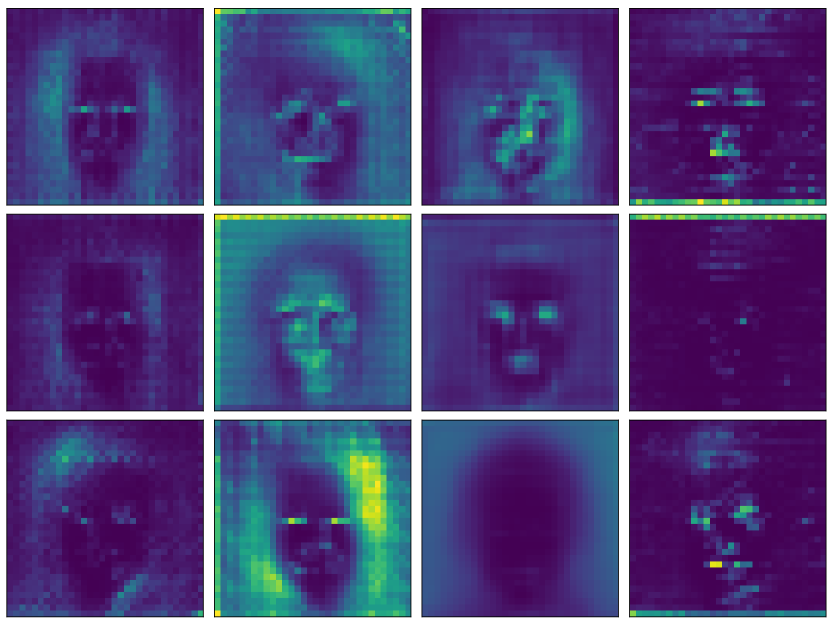
Figure 8: Average activations of DCGAN, WGAN-GP, LSGAN, EBGAN (from left to right) trained on CelebA. The rows depict the average last activation over the 6th, 22th, and 29th activation channel.

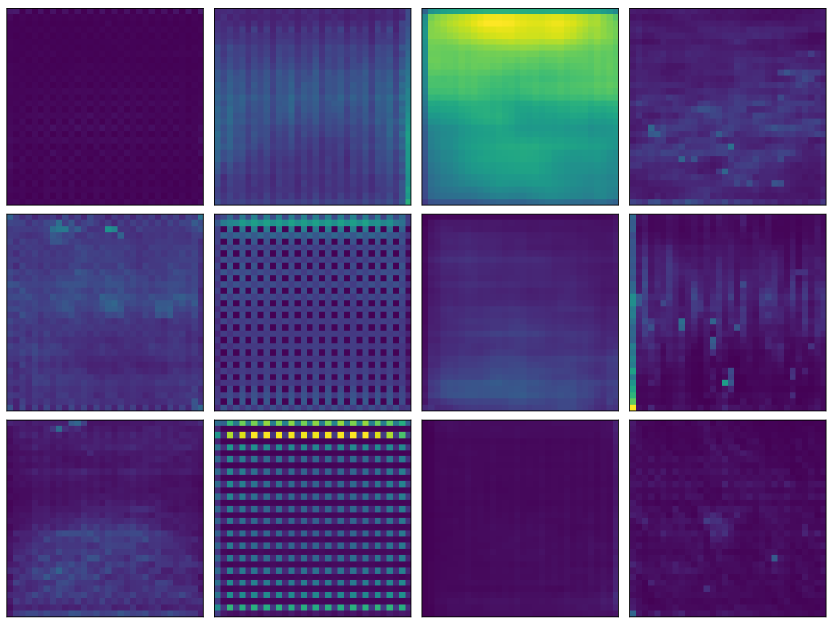
Figure 9: Average activations of DCGAN, WGAN-GP, LSGAN, EBGAN (from left to right) trained on LSUN. The rows depict the average last activation over the 7th, 29th, and 30th activation channel.

Figure 10: Average activations of Stable Diffusion v1-1, v1-1+, v1-4, v2, v2-1 (from left to right). The rows depict the average last activation over the 60th, 78th, and 86th activation channel.

Feature Extraction

We visualize the average images (Figure 11), that is, the average of the input of RawPAD, and the average DCT-features (Figure 12), that is, the average of the input of DCTPAD. It is seen that the averaged images look very similar. Qualitatively, FLIPAD improves on that as demonstrated in Figure 4 in the main paper, and once more, in Figure 13. Furthermore, the features remain distinguishable even when varying the regularization parameter $\lambda$ as visualized in Figure 14 and Figure 15. For illustration purposes, we select the 3 channel dimensions (out of 64 total activation dimensions in DCGAN), which differ the most during training, i.e. we choose the channel that maximizes the channel-wise average distance between reconstructed DCGAN and real images. Notably, the corresponding average single-model attribution accuracies are $99.11,\,99.10,\,99.44,\,86.84$ in CelebA and $99.99,\,96.58,\,99.63,\,85.90$ for $\lambda\in\{0.0001,0.0005,0.001,0.1\}$. Therefore, the performance remains stable in $\lambda$.

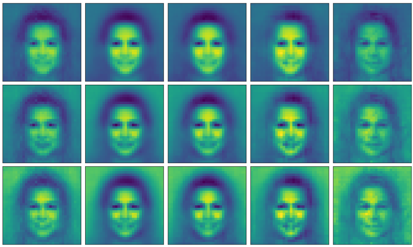
Figure 11: Average image on CelebA for real, DCGAN, WGAN-GP, LSGAN, and EBGAN samples (from left to right). Each row represents one color channel.

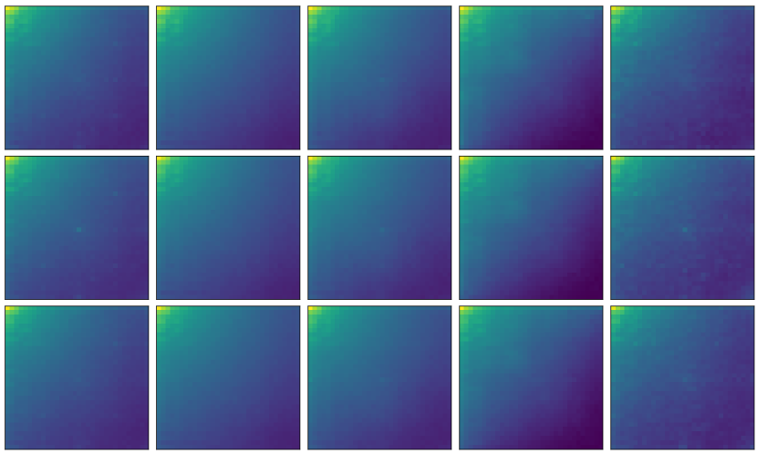
Figure 12: Average DCT-features on CelebA for real, DCGAN, WGAN-GP, LSGAN, and EBGAN samples (from left to right). Each row represents one color channel.

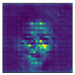
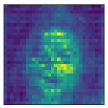
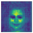
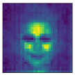
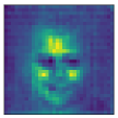
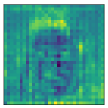
Figure 13: Cherry-picked channel dimension $c$ of the average reconstructed features according to (5) when $G$ is a DCGAN. The left-most figure shows the average activation $\bar{z}_{c}$ over channel $c$, the remaining figures show the average feature taken over DCGAN, real, WGAN-GP, LSGAN, and EBGAN samples, respectively.

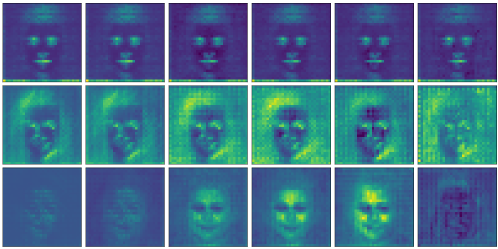
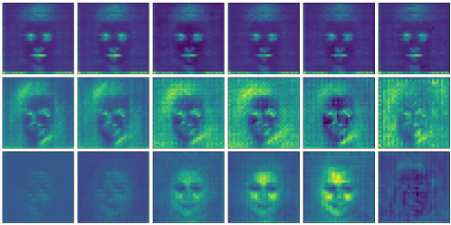
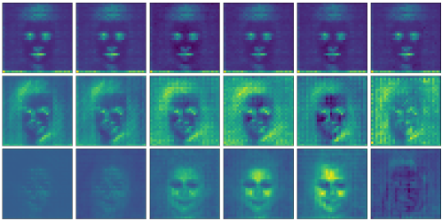
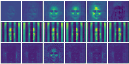
Figure 14: Average reconstructed features according to (5) when $G$ is a DCGAN trained on CelebA. Each subfigure, from top to bottom, represents the reconstructed features for a different regularization parameter $\lambda\in\{0.0001,\,0.0005,\,0.001,\,0.1\}$, respectively. Every line represents one activation channel, and the columns (from left to right) show averages taken over real activations and reconstructed DCGAN, real, WGAN-GP, LSGAN, and EBGAN activations, respectively.

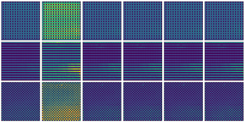
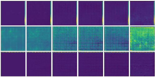
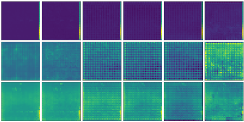
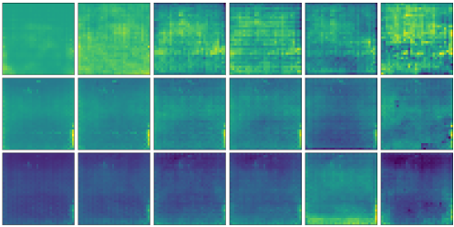
Figure 15: Average reconstructed features according to (5) when $G$ is a DCGAN trained on LSUN. Each subfigure, from top to bottom, represents the reconstructed features for a different regularization parameter $\lambda\in\{0.0001,\,0.0005,\,0.001,\,0.1\}$, respectively. Every line represents one activation channel, and the columns (from left to right) show averages taken over real activations and reconstructed DCGAN, real, WGAN-GP, LSGAN, and EBGAN activations, respectively.

Single-Model Attribution

We provide a more detailed view of the experiments from Table 1 by providing a confusion matrix in Table 7. Furthermore, we present the corresponding AUCs in Table 8. However, we want to highlight that those results should be taken with a grain of salt since AUC is measuring an overly optimistic potential of a classifier. In practice, we rely on a specific choice of threshold $\tau$ which might deteriorate the actual attribution performance. Choosing that threshold becomes even more crucial in the open-world setting, in which we do not have any access to the other models we test against, making the calibration of the threshold using only validation data considerably more difficult.

We report standard deviations to the experiments from the main paper in Table 9, 10, and 12.

	CelebA						LSUN
	Real	DCGAN	WGAN-GP	LSGAN	EBGAN		Real	DCGAN	WGANGP	LSGAN	EBGAN
SM-F
DCGAN	64.82	-	67.64	66.18	60.61		70.06	-	69.34	70.74	69.63
WGAN-GP	50.31	49.97	-	50.31	50.13		53.07	52.92	-	52.52	53.31
LSGAN	53.70	52.18	54.01	-	54.37		56.28	57.31	56.92	-	54.67
EBGAN	96.28	92.19	96.56	98.07	-		75.10	74.68	74.48	74.07	-
$\text{SM-Inv}_{2}$
DCGAN	99.55	-	99.45	99.55	95.55		51.20	-	52.00	51.05	51.50
WGAN-GP	99.80	99.80	-	99.80	99.80		50.15	49.95	-	50.20	50.50
LSGAN	71.40	59.65	67.90	-	51.25		67.20	64.50	65.30	-	64.85
EBGAN	99.80	99.80	99.80	99.80	-		54.80	53.25	55.15	54.20	-
$\text{SM-Inv}_{\operatorname{inc}}$
DCGAN	51.45	-	51.10	51.25	51.10		50.80	-	50.65	50.50	50.50
WGAN-GP	50.15	50.10	-	50.25	50.15		50.65	50.30	-	50.15	50.30
LSGAN	53.30	52.50	52.90	-	51.85		52.15	51.05	51.10	-	52.15
EBGAN	79.65	73.25	79.25	81.70	-		52.30	51.90	52.35	51.95	-
RawPAD
DCGAN	98.23	-	98.03	96.92	86.63		69.30	-	66.61	62.15	70.52
WGAN-GP	65.45	60.18	-	59.78	51.08		52.96	51.20	-	52.87	52.41
LSGAN	99.65	99.50	99.65	-	99.33		98.23	97.98	98.33	-	98.33
EBGAN	99.65	99.26	99.59	99.67	-		94.53	94.10	93.79	93.40	-
DCTPAD
DCGAN	99.81	-	80.20	95.44	49.86		99.64	-	74.98	96.96	50.34
WGAN-GP	99.68	49.71	-	60.70	49.71		99.04	49.71	-	73.91	49.73
LSGAN	99.70	98.74	96.34	-	92.39		97.95	52.44	67.15	-	54.18
EBGAN	99.66	70.39	98.69	99.59	-		99.65	65.93	96.45	99.59	-
FLIPAD
DCGAN	99.72	-	99.72	99.72	98.21		99.69	-	99.69	99.66	91.95
WGAN-GP	99.83	99.15	-	98.80	99.83		99.65	98.71	-	99.27	93.29
LSGAN	99.68	99.38	97.95	-	98.77		99.57	98.86	96.00	-	98.32
EBGAN	99.68	99.68	99.68	99.68	-		99.68	98.49	99.67	99.68	-

Table 7: Confusion Matrices corresponding to the results in Table 1. Each score corresponds to an average over five runs. Note, due to their excessive computational load, we do not repeat the inversion methods multiple times.

	CelebA					LSUN
	DCGAN	WGAN-GP	LSGAN	EBGAN		DCGAN	WGANGP	LSGAN	EBGAN
SM-F	95.45	79.09	87.94	99.84		96.99	79.09	86.73	98.36
$\text{SM-Inv}_{2}$	99.42	100.00	99.25	100.00		71.64	80.36	99.33	97.66
$\text{SM-Inv}_{\operatorname{inc}}$	83.14	67.39	85.66	99.25		61.12	55.71	74.31	92.28
RawPAD	99.33	85.03	99.99	99.96		93.82	74.65	99.83	99.53
DCTPAD	82.85	75.69	99.80	97.47		84.89	79.22	82.91	94.31
FLIPAD	99.91	99.96	99.91	100.00		99.81	99.49	99.73	99.98

Table 8: Averaged area under curve (AUC) values corresponding to the results in Table 1.

	CelebA					LSUN
	DCGAN	WGAN-GP	LSGAN	EBGAN		DCGAN	WGAN-GP	LSGAN	EBGAN
SM-F	2.95	0.26	0.95	2.81		1.60	0.87	1.65	4.16
$\text{SM-Inv}_{2}$	1.98	0.00	9.00	0.00		0.42	0.23	1.20	0.83
$\text{SM-Inv}_{\operatorname{inc}}$	0.17	0.06	0.62	3.64		0.14	0.21	0.62	0.23
RawPAD	5.53	5.60	0.20	0.21		3.79	1.08	0.34	1.66
DCTPAD	20.09	21.11	2.93	12.95		20.43	21.04	18.76	14.57
FLIPAD	0.73	0.56	0.92	0.07		4.48	2.79	1.54	0.58

Table 9: Standard deviation corresponding to the results from Table 1. For illustration purposes, we scale all values by $10^{2}$.

	CelebA					LSUN
	DCGAN	WGAN-GP	LSGAN	EBGAN		DCGAN	WGANGP	LSGAN	EBGAN
RawPAD	2.21	3.11	1.23	15.72		3.29	0.88	5.04	3.73
DCTPAD	0.27	0.14	4.31	4.13		0.19	2.33	1.05	1.42
FLIPAD	0.61	5.49	3.85	0.11		2.32	3.77	5.41	9.61

Table 10: Standard deviation corresponding to the results from Table 2. For illustration purposes, we scale all values by $10^{2}$.

Single-Model Attribution on Perturbed Samples

To illustrate the effect of the considered perturbations on the images, we present an overview in Figure 16. We observed that we can improve the attribution performance of our proposed methods by choosing the thresholding method more liberal. Specifically, in the presence of perturbations, we can set $\operatorname{fnr}=0.05$ to find $\tau$ (compare with Section F.1). We provide the improved results in Table 11.

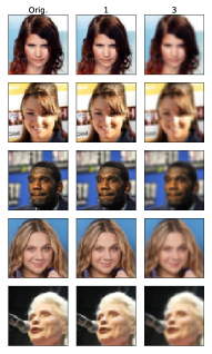
(a) Blur CelebA

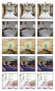
(b) Blur LSUN

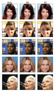
(c) Crop CelebA

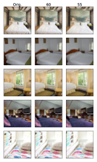
(d) Crop LSUN

(e) JPEG CelebA

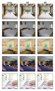
(f) JPEG LSUN

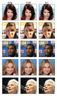
(g) Noise CelebA

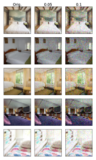
(h) Noise LSUN

Figure 16: Visualization of different perturbations.

	CelebA									LSUN
	Blur		Crop		Noise		JPEG			Blur		Crop		Noise		JPEG
	1	3	60	55	0.05	0.1	90	80		1	3	60	55	0.05	0.1	90	80
RawPAD	90.90	90.03	91.15	91.27	87.67	83.68	89.72	89.14		83.95	83.05	83.59	82.61	80.73	77.78	82.44	81.90
DCTPAD	83.35	80.19	83.34	83.33	70.86	64.02	76.49	74.98		79.09	73.08	79.26	78.28	55.04	52.20	61.97	57.80
FLIPAD	97.40	97.52	97.23	97.29	82.15	73.76	88.18	84.12		96.58	96.78	96.12	95.22	78.73	60.47	85.50	81.42

Table 11: Single-model attribution accuracy with immunization averaged over all $G,G’\in\mathcal{G}$ over five runs using a more liberal thresholding selection ($\operatorname{fnr}=0.05$). We use the same perturbations as in Table 3.

	Stable Diffusion					Style-Based Models					Medical Image Models
	v1-4	v1-1	v1-1+	v2		real	StyleGAN-XL	StyleNAT	StyleSwin		WGAN-GP	C-DCGAN
SM-F	0.00	0.00	0.00	0.00		0.00	0.00	0.00	0.00		0.10	0.10
RawPAD	4.10	3.36	1.35	0.71		4.10	3.36	2.89	1.75		0.12	19.76
DCTPAD	1.32	1.24	0.29	0.29		0.07	0.07	0.16	0.08		0.18	17.97
FLIPAD	1.35	1.04	1.19	1.56		-	-	-	-		0.11	0.19

Table 12: Standard deviation corresponding to the results from Table 4. For illustration purposes, we scale all values by $10^{2}$.

Generative Models for Tabular Data

In addition to the models trained on Redwine, we repeat the experiments for models trained on the Whitewine dataset (Cortez et al. 2009). The results are reported in Table 13. Here, we can see a different behavior: $\text{SM-Inv}_{2}$ outperforms RawPAD and FLIPAD. Moreover, we observe in our experiments that FLIPAD tends to perform better when $\lambda$ approaches $0$. This behavior suggests that it might be less meaningful to regularize towards the mean activation in the Whitewine experiments. Investigating other types of regularization in (5), however, is out of the scope of this work.

We report the corresponding standard deviations in Table 14.

	TVAE	CTGAN	Cop.GAN
$\text{SM-Inv}_{2}$	95.69	96.38	96.21
RawPAD	84.22	80.85	81.44
FLIPAD	84.15	80.58	80.84

Table 13: Single-model attribution accuracy of KL-WGAN trained on Whitewine against $G’$ as indicated by the column name averaged over five runs.

	Redwine				Whitewine
	TVAE	CTGAN	Cop.GAN		TVAE	CTGAN	Cop.GAN
$\text{SM-Inv}_{2}$	16.51	12.50	14.61		18.87	16.23	13.53
RawPAD	14.89	8.37	21.20		13.29	15.44	13.17
FLIPAD	12.50	5.57	18.37		12.82	16.48	11.17

Table 14: Standard deviation corresponding to the results from Table 5 and Table 13. For illustration purposes, we scale all values by $10^{3}$.

References

- Adi et al. (2018) Adi, Y.; Baum, C.; Cisse, M.; Pinkas, B.; and Keshet, J. 2018. Turning Your Weakness into a Strength: Watermarking Deep Neural Networks by Backdooring. In Proceedings of the 27th USENIX Conference on Security Symposium, SEC’18, 1615–1631. USA: USENIX Association. ISBN 9781931971461.
- Albright and McCloskey (2019) Albright, M.; and McCloskey, S. 2019. Source Generator Attribution via Inversion. In Proceedings of the IEEE/CVF Conference on Computer Vision and Pattern Recognition Workshops, 96–103.
- Alyafi, Diaz, and Marti (2020) Alyafi, B.; Diaz, O.; and Marti, R. 2020. DCGANs for realistic breast mass augmentation in x-ray mammography. In Medical Imaging 2020: Computer-Aided Diagnosis, volume 11314, 473–480. SPIE.
- Bandeira et al. (2013) Bandeira, A. S.; Dobriban, E.; Mixon, D. G.; and Sawin, W. F. 2013. Certifying the restricted isometry property is hard. IEEE transactions on information theory, 59(6): 3448–3450.
- Baraniuk et al. (2008) Baraniuk, R.; Davenport, M. A.; DeVore, R. A.; and Wakin, M. B. 2008. A Simple Proof of the Restricted Isometry Property for Random Matrices. Constructive Approximation, 28: 253–263.
- Beck and Teboulle (2009) Beck, A.; and Teboulle, M. 2009. A fast iterative shrinkage-thresholding algorithm for linear inverse problems. SIAM journal on imaging sciences, 2(1): 183–202.
- Brown et al. (2020) Brown, T.; Mann, B.; Ryder, N.; Subbiah, M.; Kaplan, J. D.; Dhariwal, P.; Neelakantan, A.; Shyam, P.; Sastry, G.; Askell, A.; Agarwal, S.; Herbert-Voss, A.; Krueger, G.; Henighan, T.; Child, R.; Ramesh, A.; Ziegler, D.; Wu, J.; Winter, C.; Hesse, C.; Chen, M.; Sigler, E.; Litwin, M.; Gray, S.; Chess, B.; Clark, J.; Berner, C.; McCandlish, S.; Radford, A.; Sutskever, I.; and Amodei, D. 2020. Language Models are Few-Shot Learners. In Larochelle, H.; Ranzato, M.; Hadsell, R.; Balcan, M.; and Lin, H., eds., Advances in Neural Information Processing Systems, volume 33, 1877–1901. Curran Associates, Inc.
- Candès (2008) Candès, E. J. 2008. The restricted isometry property and its implications for compressed sensing. Comptes Rendus Mathematique, 346(9): 589–592.
- Chen, Donoho, and Saunders (2001) Chen, S. S.; Donoho, D. L.; and Saunders, M. A. 2001. Atomic Decomposition by Basis Pursuit. SIAM review, 43(1): 129–159.
- Cortez et al. (2009) Cortez, P.; Cerdeira, A.; Almeida, F.; Matos, T.; and Reis, J. 2009. Modeling wine preferences by data mining from physicochemical properties. Decision Support Systems, 47(4): 547–553. Smart Business Networks: Concepts and Empirical Evidence.
- Eldar and Kutyniok (2012) Eldar, Y. C.; and Kutyniok, G. 2012. Compressed sensing: theory and applications. Cambridge university press.
- Frank et al. (2020) Frank, J.; Eisenhofer, T.; Schönherr, L.; Fischer, A.; Kolossa, D.; and Holz, T. 2020. Leveraging Frequency Analysis for Deep Fake Image Recognition. In Proceedings of the 37th International Conference on Machine Learning, volume 119 of Proceedings of Machine Learning Research, 3247–3258.
- Girish et al. (2021) Girish, S.; Suri, S.; Rambhatla, S. S.; and Shrivastava, A. 2021. Towards Discovery and Attribution of Open-world GAN Generated Images. In Proceedings of the IEEE/CVF International Conference on Computer Vision, 14094–14103.
- Gulrajani et al. (2017) Gulrajani, I.; Ahmed, F.; Arjovsky, M.; Dumoulin, V.; and Courville, A. C. 2017. Improved training of wasserstein gans. Advances in neural information processing systems, 30.
- Haupt et al. (2010) Haupt, J.; Bajwa, W. U.; Raz, G.; and Nowak, R. 2010. Toeplitz Compressed Sensing Matrices With Applications to Sparse Channel Estimation. IEEE Transactions on Information Theory, 56(11): 5862–5875.
- Hefferon (2012) Hefferon, J. 2012. Linear Algebra.
- Hirofumi et al. (2022) Hirofumi, S.; Fukuchi, K.; Akimoto, Y.; and Sakuma, J. 2022. Did You Use My GAN to Generate Fake? Post-hoc Attribution of GAN Generated Images via Latent Recovery. In 2022 International Joint Conference on Neural Networks (IJCNN), 1–8.
- Karras et al. (2021) Karras, T.; Aittala, M.; Laine, S.; Härkönen, E.; Hellsten, J.; Lehtinen, J.; and Aila, T. 2021. Alias-free generative adversarial networks. Advances in Neural Information Processing Systems, 34: 852–863.
- Karras, Laine, and Aila (2019) Karras, T.; Laine, S.; and Aila, T. 2019. A style-based generator architecture for generative adversarial networks. In Proceedings of the IEEE/CVF conference on computer vision and pattern recognition, 4401–4410.
- Karras et al. (2020) Karras, T.; Laine, S.; Aittala, M.; Hellsten, J.; Lehtinen, J.; and Aila, T. 2020. Analyzing and Improving the Image Quality of StyleGAN. In Proceedings of the IEEE/CVF Conference on Computer Vision and Pattern Recognition (CVPR).
- Kim, Ren, and Yang (2021) Kim, C.; Ren, Y.; and Yang, Y. 2021. Decentralized Attribution of Generative Models. In International Conference on Learning Representations.
- Kingma and Ba (2015) Kingma, D. P.; and Ba, J. 2015. Adam: A Method for Stochastic Optimization. In International Conference on Learning Representations.
- Krahmer, Mendelson, and Rauhut (2013) Krahmer, F.; Mendelson, S.; and Rauhut, H. 2013. The restricted isometry property for random convolutions. International Conference on Sampling Theory and Applications, 10: 376–379.
- Lago et al. (2022) Lago, F.; Pasquini, C.; Böhme, R.; Dumont, H.; Goffaux, V.; and Boato, G. 2022. More Real Than Real: A Study on Human Visual Perception of Synthetic Faces [Applications Corner]. IEEE Signal Processing Magazine, 39(1): 109–116.
- Lederer (2022a) Lederer, J. 2022a. Fundamentals of High-Dimensional Statistics: With Exercises and R Labs. Springer Texts in Statistics. ISBN 978-3-030-73792-4.
- Lederer (2022b) Lederer, J. 2022b. Statistical guarantees for sparse deep learning. arXiv preprint arXiv:2212.05427.
- Li (2020) Li, C. 2020. OpenAI’s GPT-3 Language Model: A Technical Overview. https://lambdalabs.com/blog/demystifying-gpt-3.
- Lin et al. (2014) Lin, T.-Y.; Maire, M.; Belongie, S.; Hays, J.; Perona, P.; Ramanan, D.; Dollár, P.; and Zitnick, C. L. 2014. Microsoft COCO: Common Objects in Context. In Fleet, D.; Pajdla, T.; Schiele, B.; and Tuytelaars, T., eds., Computer Vision – ECCV 2014, 740–755. Cham: Springer International Publishing.
- Liu et al. (2015) Liu, Z.; Luo, P.; Wang, X.; and Tang, X. 2015. Deep Learning Face Attributes in the Wild. In Proceedings of International Conference on Computer Vision (ICCV).
- Lopez et al. (2012) Lopez, M. A. G.; Posada, N.; Moura, D. C.; Pollán, R. R.; Jose, M. G.-V.; Valiente, F. S.; Ortega, C. S.; del Solar, M. R.; Herrero, G. D.; IsabelM., A.; Ramos, P.; Loureiro, J.; Fernandes, T. C.; and de Araújo, B. M. F. 2012. BCDR : A BREAST CANCER DIGITAL REPOSITORY.
- Mao et al. (2017) Mao, X.; Li, Q.; Xie, H.; Lau, R. Y.; Wang, Z.; and Paul Smolley, S. 2017. Least squares generative adversarial networks. In Proceedings of the IEEE international conference on computer vision, 2794–2802.
- Marra et al. (2019a) Marra, F.; Gragnaniello, D.; Verdoliva, L.; and Poggi, G. 2019a. Do GANs Leave Artificial Fingerprints? In 2019 IEEE Conference on Multimedia Information Processing and Retrieval (MIPR), 506–511.
- Marra et al. (2019b) Marra, F.; Saltori, C.; Boato, G.; and Verdoliva, L. 2019b. Incremental Learning for the Detection and Classification of GAN-generated Images. In 2019 IEEE International Workshop on Information Forensics and Security (WIFS), 1–6.
- Mink et al. (2022) Mink, J.; Luo, L.; Barbosa, N. M.; Figueira, O.; Wang, Y.; and Wang, G. 2022. DeepPhish: Understanding User Trust Towards Artificially Generated Profiles in Online Social Networks. In 31st USENIX Security Symposium (USENIX Security 22), 1669–1686. Boston, MA: USENIX Association. ISBN 978-1-939133-31-1.
- Nightingale and Farid (2022) Nightingale, S. J.; and Farid, H. 2022. AI-synthesized faces are indistinguishable from real faces and more trustworthy. Proceedings of the National Academy of Sciences, 119(8): e2120481119.
- Ong et al. (2021) Ong, D. S.; Chan, C. S.; Ng, K. W.; Fan, L.; and Yang, Q. 2021. Protecting intellectual property of generative adversarial networks from ambiguity attacks. In Proceedings of the IEEE/CVF Conference on Computer Vision and Pattern Recognition, 3630–3639.
- Osuala et al. (2023) Osuala, R.; Skorupko, G.; Lazrak, N.; Garrucho, L.; García, E.; Joshi, S.; Jouide, S.; Rutherford, M.; Prior, F.; Kushibar, K.; et al. 2023. medigan: a Python library of pretrained generative models for medical image synthesis. Journal of Medical Imaging, 10(6): 061403.
- Parhi and Nowak (2021) Parhi, R.; and Nowak, R. D. 2021. Banach Space Representer Theorems for Neural Networks and Ridge Splines. J. Mach. Learn. Res., 22(43): 1–40.
- Patki, Wedge, and Veeramachaneni (2016) Patki, N.; Wedge, R.; and Veeramachaneni, K. 2016. The Synthetic data vault. In IEEE International Conference on Data Science and Advanced Analytics (DSAA), 399–410.
- Radford, Metz, and Chintala (2015) Radford, A.; Metz, L.; and Chintala, S. 2015. Unsupervised representation learning with deep convolutional generative adversarial networks. arXiv preprint arXiv:1511.06434.
- Ramesh et al. (2022) Ramesh, A.; Dhariwal, P.; Nichol, A.; Chu, C.; and Chen, M. 2022. Hierarchical Text-Conditional Image Generation with CLIP Latents.
- Rea (2023) Rea, N. 2023. Could a Robot Ever Recreate the Aura of a Leonardo Da Vinci Masterpiece? It’s Already Happening. The Guardian.
- Rombach et al. (2022) Rombach, R.; Blattmann, A.; Lorenz, D.; Esser, P.; and Ommer, B. 2022. High-Resolution Image Synthesis With Latent Diffusion Models. In Proceedings of the IEEE/CVF Conference on Computer Vision and Pattern Recognition (CVPR), 10684–10695.
- Ruff et al. (2018) Ruff, L.; Vandermeulen, R.; Goernitz, N.; Deecke, L.; Siddiqui, S. A.; Binder, A.; Müller, E.; and Kloft, M. 2018. Deep One-Class Classification. In Dy, J.; and Krause, A., eds., Proceedings of the 35th International Conference on Machine Learning, volume 80 of Proceedings of Machine Learning Research, 4393–4402. PMLR.
- Ruff et al. (2019) Ruff, L.; Vandermeulen, R. A.; Görnitz, N.; Binder, A.; Müller, E.; Müller, K.-R.; and Kloft, M. 2019. Deep semi-supervised anomaly detection. arXiv preprint arXiv:1906.02694.
- Saharia et al. (2022) Saharia, C.; Chan, W.; Saxena, S.; Li, L.; Whang, J.; Denton, E.; Ghasemipour, S. K. S.; Ayan, B. K.; Mahdavi, S. S.; Lopes, R. G.; Salimans, T.; Ho, J.; Fleet, D. J.; and Norouzi, M. 2022. Photorealistic Text-to-Image Diffusion Models with Deep Language Understanding.
- Sauer, Schwarz, and Geiger (2022) Sauer, A.; Schwarz, K.; and Geiger, A. 2022. Stylegan-xl: Scaling stylegan to large diverse datasets. In ACM SIGGRAPH 2022 conference proceedings, 1–10.
- Song and Ermon (2020) Song, J.; and Ermon, S. 2020. Bridging the gap between f-gans and wasserstein gans. In International Conference on Machine Learning, 9078–9087. PMLR.
- Szafranowska et al. (2022) Szafranowska, Z.; Osuala, R.; Breier, B.; Kushibar, K.; Lekadir, K.; and Diaz, O. 2022. Sharing generative models instead of private data: a simulation study on mammography patch classification. In 16th International Workshop on Breast Imaging (IWBI2022), volume 12286, 169–177. SPIE.
- Szegedy et al. (2016) Szegedy, C.; Vanhoucke, V.; Ioffe, S.; Shlens, J.; and Wojna, Z. 2016. Rethinking the Inception Architecture for Computer Vision. In Proceedings of the IEEE Conference on Computer Vision and Pattern Recognition (CVPR).
- Tax and Duin (2004) Tax, D. M. J.; and Duin, R. P. W. 2004. Support Vector Data Description. Machine Learning, 54: 45–66.
- Tibshirani (1996) Tibshirani, R. 1996. Regression shrinkage and selection via the lasso. Journal of the Royal Statistical Society: Series B (Methodological), 58(1): 267–288.
- Tibshirani (2013) Tibshirani, R. J. 2013. The lasso problem and uniqueness. Electronic Journal of statistics, 7: 1456–1490.
- Varoquaux and Cheplygina (2022) Varoquaux, G.; and Cheplygina, V. 2022. Machine learning for medical imaging: methodological failures and recommendations for the future. NPJ digital medicine, 5(1): 48.
- Walton et al. (2022) Walton, S.; Hassani, A.; Xu, X.; Wang, Z.; and Shi, H. 2022. StyleNAT: Giving each head a new perspective. arXiv preprint arXiv:2211.05770.
- Xu et al. (2019) Xu, L.; Skoularidou, M.; Cuesta-Infante, A.; and Veeramachaneni, K. 2019. Modeling Tabular data using Conditional GAN. In Advances in Neural Information Processing Systems.
- Xuan et al. (2019) Xuan, X.; Peng, B.; Wang, W.; and Dong, J. 2019. Scalable Fine-Grained Generated Image Classification Based on Deep Metric Learning. arXiv:1912.11082.
- Yu et al. (2015) Yu, F.; Zhang, Y.; Song, S.; Seff, A.; and Xiao, J. 2015. LSUN: Construction of a Large-scale Image Dataset using Deep Learning with Humans in the Loop. CoRR, abs/1506.03365.
- Yu, Davis, and Fritz (2019) Yu, N.; Davis, L. S.; and Fritz, M. 2019. Attributing Fake Images to GANs: Learning and Analyzing GAN Fingerprints. In Proceedings of the IEEE/CVF International Conference on Computer Vision, 7556–7566.
- Yu et al. (2021) Yu, N.; Skripniuk, V.; Abdelnabi, S.; and Fritz, M. 2021. Artificial Fingerprinting for Generative Models: Rooting Deepfake Attribution in Training Data. In Proceedings of the IEEE/CVF International Conference on Computer Vision, 14448–14457.
- Yu et al. (2022) Yu, N.; Skripniuk, V.; Chen, D.; Davis, L. S.; and Fritz, M. 2022. Responsible Disclosure of Generative Models Using Scalable Fingerprinting. International Conference on Learning Representations.
- Zhang et al. (2022) Zhang, B.; Gu, S.; Zhang, B.; Bao, J.; Chen, D.; Wen, F.; Wang, Y.; and Guo, B. 2022. Styleswin: Transformer-based gan for high-resolution image generation. In Proceedings of the IEEE/CVF conference on computer vision and pattern recognition, 11304–11314.
- Zhang et al. (2021) Zhang, B.; Zhou, J. P.; Shumailov, I.; and Papernot, N. 2021. On Attribution of Deepfakes. arXiv:2008.09194 [cs].
- Zhao, Mathieu, and LeCun (2016) Zhao, J.; Mathieu, M.; and LeCun, Y. 2016. Energy-based generative adversarial network. arXiv preprint arXiv:1609.03126.