New Calabi–Yau Manifolds from Genetic Algorithms

Abstract

Calabi–Yau manifolds can be obtained as hypersurfaces in toric varieties built from reflexive polytopes. We generate reflexive polytopes in various dimensions using a genetic algorithm. As a proof of principle, we demonstrate that our algorithm reproduces the full set of reflexive polytopes in two and three dimensions, and in four dimensions with a small number of vertices and points. Motivated by this result, we construct five-dimensional reflexive polytopes with the lowest number of vertices and points. By calculating the normal form of the polytopes, we establish that many of these are not in existing datasets and therefore give rise to new Calabi–Yau four-folds. In some instances, the Hodge numbers we compute are new as well.

1 Introduction

Ever since the early days of string phenomenology Candelas:1985en , the construction of Calabi–Yau (CY) manifolds had been an active pursuit in the theoretical physics and mathematics communities. (See, for example, the classic reference Hubsch:1992nu as well as the recent textbooks He:2018jtw ; Bao:2020sqg .) This is motivated by the existence of Ricci-flat metrics on CY manifolds, a property which makes them a useful building block for compactifications of string theory. In particular, CY three-folds compactify ten-dimensional superstring theory to four-dimensional quantum field theories with $\mathcal{N}=1$ supersymmetry Candelas:1985en .

In a parallel, and initially seemingly unrelated, vein, lattice polytopes play a central role in geometry, where a polytope defines a fan of strongly convex rational polyhedra cones which in turn defines a toric variety. In batyrev1993dual ; batyrev1994calabiyau , Batyrev and Borisov showed how mirror pairs of $(n-1)$ complex dimensional CY manifolds can be realized from hypersurfaces in toric varieties constructed from $n$-dimensional reflexive polytopes.

Threading these two directions of CY compactifications and toric hypersurfaces, and motivated by their utility for string phenomenology, Kreuzer and Skarke devised an algorithm to generate all reflexive polytopes in $n$ dimensions Kreuzer_1997 . The algorithm consists of two steps. First, a set $S$ of “maximal” polytopes is constructed such that any reflexive polytope is a subpolytope of a polytope in $S$. These maximal polytopes are defined by a so-called “weight system” or a combination of weight systems. Second, all subpolyhedra of all polyhedra in $S$ are constructed and checked for reflexivity. The complete classification of $4319$ three-dimensional reflexive polytopes with this algorithm was accomplished in kreuzer1998classification . From these we obtain K3 surfaces, which is to say, CY two-folds. Proceeding to dimension three, the $184,026$ weight systems giving rise to four-dimensional reflexive polytopes were presented in skarke_1996 , and the resulting $473,800,776$ four-dimensional reflexive polytopes, leading to CY three-folds, were listed in kreuzer2000complete . In five dimensions the total number of reflexive polytopes is prohibitively large, and Schöller and Skarke were only able to run the first stage of the algorithm to calculate all $322,383,760,930$ weight systems corresponding to maximal polytopes Sch_ller_2019 . They found that $185,269,499,015$ of these weight systems give rise to reflexive polytopes directly. This result constitutes a partial classification, and we will compare our results to this list later on. The CY four-folds obtained from five-dimensional reflexive polytopes facilitate F-theory model building.

Finding reflexive polytopes is not an easy task. A lattice polytope is reflexive when it satisfies a set of conditions: it must have only a single interior point (the so-called IP property), its dual must as well be a lattice polytope (that is, its vertices must lie on integer lattice points), and the dual must also satisfy the IP property. Alternatively and equivalently, a polytope is reflexive if and only if it satisfies the IP property and all bounding hyperplanes of the polytope lie at unit hyperplane distance from the origin. Constructing polytopes is a well defined problem in Big Data. With multiple criteria, regression is unlikely to perform well at finding reflexive polytopes. Any loss function will have local minima, where polytopes satisfy some but not all of the conditions for reflexivity. We can ask if methods such as reinforcement learning or genetic algorithms, which explore an “environment” in order to maximize a fitness or reward function, might be better suited for such a task. In this paper, we will address this question for genetic algorithms (GAs) and leave reinforcement learning for future work. Significant work has already been done on applying machine learning techniques to study objects in string theory, including polytopes bao2021polytopes ; Berman:2021mcw ; Berglund:2021ztg . Genetic algorithms in particular have been successful at scanning for phenomenologically attractive string models Abel_2014 ; abel2021string and cosmic inflation models Abel_2022 , but this is the first time that genetic algorithms have been used to search for reflexive polytopes. We note that work has been done on generating reflexive polytopes using sequential models with the added condition that the polytopes are also regular nodland2022 . However, applying this methodology to reflexive polytopes without the regularity condition does not yield good results.

The organization of this paper is as follows. In Sections 2.1 and 2.2, we present some background on reflexive polytopes and briefly review genetic algorithms. In Section 3, we describe our methodology for searching for reflexive polytopes with GAs. Section 4 presents the results of our GA searches for reflexive polytopes in two, three, and four dimensions and compares the results to the known complete classifications. Five-dimensional reflexive polytopes are tackled in Section 5. Using GAs, we generate datasets of five-dimensional reflexive polytopes with the smallest number of points and vertices. From these we extract the polytopes with $h^{1,1}=1$ and $h^{1,1}=2$ and compare with the existing partial classification. We conjecture that there are exactly $15$ five-dimensional reflexive polytopes that have $h^{1,1}=1$. We also present an example of a targeted search where conditions are placed on the Euler number of the CY manifold. In Section 6, we finish with a discussion and prospectus. Our code, along with a database of five-dimensional reflexive polytopes we have generated is available on GitHub githubcGA ; Reflexive_Polytope_Genetic .

2 Background

In this section we briefly review the necessary background, both on the mathematics of lattice polytopes and on GAs, while leaving some of the technical details to the appendices.

2.1 Reflexive polytopes

Due to theorems of Batyrev and Borisov batyrev1993dual ; batyrev1994calabiyau reflexive polytopes provide an efficient way to construct Calabi–Yau (CY) manifolds. (See Appendix A for a short review.) This close connection to CY manifolds is the principal reason why physicists are interested in reflexive polytopes, and it prompted Kreuzer and Skarke to perform a tour de force computer classification Kreuzer_1997 ; kreuzer1998classification ; kreuzer2000complete which produced the largest available databases of smooth, compact CY manifolds in complex dimensions two and three.

Let us briefly review some of the properties of lattice polytopes relevant to our work. An $n$-dimensional lattice polytope $\Delta$ is the convex hull in $\mathbb{R}^{n}$ of a finite number of lattice points $x_{1},\ldots,x_{m}\in\mathbb{Z}^{n}\subset\mathbb{R}^{n}$. These points can be conveniently combined into an $n\times m$ matrix ${\mathcal{X}}=(x_{1},\ldots,x_{m})$ whose columns are the generators. The vertices $v_{1},\ldots,v_{N_{\text{v}}}$ of $\Delta$ are a subset of the lattice points $x_{i}$, so that $N_{\text{v}}=N_{\text{v}}(\Delta)\leq m$. The vertices can also be combined into an $n\times N_{v}$ vertex matrix $V=(v_{1},\ldots,v_{N_{v}})$. Let $H=\{x\in\mathbb{R}^{n}\,|\,u\cdot x=d\}$ be a hyperplane where $u\in\mathbb{Z}^{n}$ is a primitive lattice point and $d\in\mathbb{R}$. Such a hyperplane is called valid if the polytope $\Delta$ is contained in the associated negative half-space, that is, if $u\cdot x\leq d$ for all $x\in\Delta$. A face of $\Delta$ is the intersection of $\Delta$ with a valid hyperplane, and a facet is a face of dimension $n-1$. We denote the set of all facets by $F(\Delta)$ and for a facet $\varphi\in F(\Delta)$ with equation $u\cdot x=d$ (where $u$ is a primitive lattice point) the number $d=d_{\Delta}(\varphi)$ is called the lattice distance of $\varphi$ from the origin. It is also useful to introduce the notation $N_{\text{p}}(\Delta)$ for the number of lattice points in $\Delta$.

As explained in Appendix A, a lattice polytope is said to have the IP property if the origin is its only interior lattice point. Furthermore, $\Delta$ is called reflexive if it has the IP property and if its dual polytope $\Delta^{*}$ is also a lattice polytope and has the IP property. Equivalently, $\Delta$ is reflexive if and only if it has the IP property and if all its facets have lattice distance one, that is, if $d_{\Delta}(\varphi)=1$ for all $\varphi\in F(\Delta)$. It is the latter characterization of reflexivity which we will use later in our definition of the fitness function.

We consider two polytopes $\Delta$ and $\widetilde{\Delta}$ with the same number of vertices, $N_{\text{v}}(\Delta)=N_{\text{v}}(\widetilde{\Delta})=N_{\text{v}}$, as equivalent if their vertices are related by a common integer linear transformation combined with a permutation. In other words, $\Delta$ and $\widetilde{\Delta}$ are equivalent if there exist an $N_{\text{v}}\times N_{\text{v}}$ permutation matrix $P$ and a $G\in\text{GL}(n,\mathbb{Z})$ such that their vertex matrices $V$ and $\widetilde{V}$ are related by

$$\widetilde{V}=G\,VP\;.$$ (1)

The most efficient way to eliminate the redundancy due to this identification is to define a normal form for the vertex matrix, thereby selecting precisely one representative per equivalence class. The definition of this normal form and an algorithm for its computation is reviewed in Appendix B. It is known that the number of reflexive polytopes, after modding out the identification (1), is finite in any given dimension $n$ lagarias_ziegler_1991 . The connection between reflexive polytopes and CYs is further discussed in Appendix A.

2.2 Genetic algorithms

Genetic algorithms (GAs) are optimization algorithms which mimic the process of natural selection darwin . They were first put forward in the 1950s turing ; barricelli and were later formalized by Holland Holland1975 . Some more recent reviews are David1989 ; Holland1992 ; Reeves2002 ; Charbonneau:2002 ; haupt ; Michalewicz2004 .

GAs operate on a certain state space which is frequently (and indeed in our applications) taken to be the set $\mathbb{F}^{n_{\text{bits}}}_{2}$ which consists of all bit lists with length $n_{\text{bits}}$. The elements of this set are often referred to as genotypes. Further, we have two given functions, a fitness function $f:\mathbb{F}^{n_{\text{bits}}}_{2}\rightarrow\mathbb{R}$ whose value the algorithm is attempting to optimize and a probability distribution $p_{\text{in}}:\mathbb{F}^{n_{\text{bits}}}_{2}\rightarrow[0,1]$, which is used to select the initial population.

The first step of a GA evolution is to select an initial population $P_{0}$ which contains a certain number, $n_{\text{pop}}$, of bit strings, each of length $n_{\text{bits}}$, by sampling the set $\mathbb{F}^{n_{\text{bits}}}_{2}$ with probability $p_{\text{in}}$. The genetic evolution then consists of a sequence

$$P_{0}\rightarrow P_{1}\rightarrow\cdots\cdots\rightarrow P_{n_{\text{gen}}-1}\rightarrow P_{n_{\text{gen}}}$$ (2)

of further $n_{\text{gen}}$ populations, each with the same size $n_{\text{pop}}$. The basic evolutionary process, $P_{k}\rightarrow P_{k+1}$, to obtain population $k+1$ from population $k$ is carried out in three steps, namely, (i) selection, (ii) cross-over, and (iii) mutation. We describe these three steps in turn.

• Selection: A probability distribution $p_{k}:P_{k}\rightarrow[0,1]$, based on the fitness function, is computed for the $k^{\text{th}}$ population. There are several ways to do this but the method we will employ here is the so-called roulette wheel selection where $p_{k}$ for an individual $s\in P_{k}$ is defined by

  $$p_{k}(s)=\frac{1}{n_{\text{pop}}}\frac{(\alpha-1)\left(f(s)-\bar{f}\right)+f_{\text{max}}-\bar{f}}{f_{\text{max}}-\bar{f}}\;,$$ (3)

  where $\bar{f}$ and $f_{\text{max}}$ are the average and maximal fitness values on $P_{k}$, respectively. The parameter $\alpha$, typically chosen in the range $\alpha\in[2,5]$, indicates by which factor the fittest individual in the population is more likely to be selected than the average one. Based on this probability $p_{k}$, $n_{\text{pop}}/2$ pairs are selected from the population $P_{k}$.

• Cross-over: For each pair selected in step (i), a random location $l\in\{1,\ldots,n_{\text{bits}}\}$ along the bit string is chosen and the tails of the two strings are swapped. Carrying this out for all pairs leads to $n_{\text{pop}}$ new bit strings, which form the precursor, $\widetilde{P}_{k+1}$, of the new population.

• Mutation: In the final step, a certain fraction, $r_{\text{mut}}$, of bits in the population $\widetilde{P}_{k+1}$ from step (ii) is flipped and this produces the next generation $P_{k+1}$.

A common addition to the above algorithm (which we employ in our applications) is elitism which means that the fittest individual from population $P_{k}$ is copied to the population $P_{k+1}$ unchanged. In summary, a GA evolution is subject to the following hyper-parameter choices: the population size $n_{\text{pop}}$, the number of generations $n_{\text{gen}}$, the parameter $\alpha$ in (3) and the mutation rate $r_{\text{mut}}$. For a systematic search, typically many GA evolutions, each with a new randomly sampled initial population $P_{0}$, are carried out. Then, the desirable (or “terminal”) states $s$, defined as states with $f(s)\geq f_{\text{term}}$ for a certain critical value $f_{\text{term}}$, are extracted from all populations which arise in this way.

3 Methodology

For our applications, we use a lightweight and fast c code githubcGA which realizes the genetic algorithm (GA).

In order to set up the environment, we consider lattice polytopes $\Delta$ in $n$ dimensions which are generated as the convex hull of $m$ vectors $x_{a}\in\mathbb{Z}^{n}$, where $a=1,\ldots,m$. These vectors are arranged into an $n\times m$ matrix ${\mathcal{X}}=(x_{1},\ldots,x_{m})$.

Standard methods can be used to calculate the properties of the polytope $\Delta$ associated to a matrix ${\mathcal{X}}$. This includes the set of facets $F(\Delta)$, the distances $d_{\Delta}(\varphi)$ of the facets $\varphi\in F(\Delta)$ from the origin, the lists of interior and all lattice points in $\Delta$, and the vertices $V=(v_{1},\ldots,v_{N_{\text{v}}(\Delta)})$. If $\Delta$ is reflexive, further interesting properties such as the Euler number $\chi(\Delta)$ and the Hodge numbers $h^{p,q}(\Delta)$ of the respective CY family can be computed. All this is carried out using the package PALP Kreuzer_2004 .

In practice, we must restrict the entries $x_{a}^{i}$ of the matrix ${\mathcal{X}}$ to a finite range which we choose to be $x_{a}^{i}\in\{x_{\text{min}},x_{\text{min}}+1,\ldots,x_{\text{min}}+2^{\nu}-1\}$, for certain integers $x_{\text{min}}$ and $\nu$. Our environment $E$ therefore consists of all $n\times m$ integer matrices ${\mathcal{X}}$ with entries in this range. The elements of an environment $E$ are also referred to as phenotypes. The first step in applying GAs to such an environment is to define the phenotype-genotype map $E\rightarrow\mathbb{F}^{n_{\text{bits}}}_{2}$. Given our choices this is quite straightforward. Each integer $x_{a}^{i}$ is converted into a bit string of length $\nu$ and concatenating these leads to a bit string of length $n_{\text{bits}}=n\,m\,\nu$ which describes the entire matrix ${\mathcal{X}}$. With these conventions the phenotype-genotype map is, in fact, bijective and the environment $E$ contains a total of

$$2^{n_{\text{bits}}}=2^{nm\nu}$$ (4)

states. To orient ourselves let us consider polytopes in dimension $n=5$ with the minimal number, $m=6$, of generators and with each integer $x_{a}^{i}$ represented by $\nu=3$ bits (so that, choosing for example $x_{\text{min}}=-4$, the integer range is $x_{a}^{i}\in\{-4,\ldots,3\}$). In this case, the environment consists of $2^{90}\simeq 10^{27}$ states, quite a sizeable number and certainly well beyond systematic search.

Next, we need to define the probability distribution $p_{\text{in}}$ and the fitness function $f$. Given the bijection between the spaces of genotypes and phenotypes these functions can be defined on either space and we opt for the latter. For the sampling probability $p_{\text{in}}$ it is usually sufficient to use a flat distribution, that is, every matrix ${\mathcal{X}}\in E$ has the same probability. Our basic fitness function is defined as

$$f(\Delta)=w_{1}\left(\text{IP}(\Delta)-1\right)-\frac{w_{2}}{|F(\Delta)|}\sum_{\varphi\in F(\Delta)}|d_{\Delta}(\varphi)-1|\;,$$ (5)

where $\text{IP}(\Delta)$ equals $1$ if $\Delta$ has the IP property and is $0$ otherwise. The numbers $w_{1},w_{2}\in\mathbb{R}^{>0}$ are weights which are typically chosen as $w_{1}=w_{2}=1$. Note that $f(\Delta)\leq 0$ always and $f(\Delta)=0$ if and only if $\Delta$ is reflexive. Accordingly, we set $f_{\text{term}}=0$ so that the terminal states correspond to reflexive polytopes.

To summarize, the GA setup for polytopes is completely specified by choosing the following environmental variables: the number of dimensions $n$, the number of generators $m$, the size $x_{\text{min}}$ of the lowest possible matrix entries, the number $\nu$ of bits used per matrix entry and the weights $w_{1}$, $w_{2}$ which appear in the fitness function (5).

For some of our applications we are interested in a more targeted search for reflexive polytopes with certain additional properties. For example, we might be interested in reflexive polytopes $\Delta$ whose number $N_{\text{p}}(\Delta)$ of lattice points equals a certain target $N_{\text{p},0}$. Another interesting subclass of reflexive polytopes are those whose number of vertices $N_{\text{v}}(\Delta)$ matches a target $N_{\text{v},0}$. To facilitate such targeted searches, we can modify the fitness function (5) to

$$\widetilde{f}(\Delta)=f(\Delta)-w_{3}\,|N_{\text{p}}(\Delta)-N_{\text{p},0}|-w_{4}\,|N_{\text{v}}(\Delta)-N_{\text{v},0}|\;,$$ (6)

where $w_{3},w_{4}\in\mathbb{R}^{\geq 0}$ are two further weights which can be used to switch the additional requirements on and off. If $w_{3},w_{4}>0$, then $\widetilde{f}(\Delta)=0$ and, hence, $\Delta$ is terminal, if and only if $\Delta$ is reflexive and has the target numbers $N_{\text{p},0}$ and $N_{\text{v},0}$ of lattice points and vertices.

This environment is realized in c by combining PALP Kreuzer_2004 tools for polytope computation with additional code by the authors Reflexive_Polytope_Genetic which realizes the phenotype-genotype conversion and the computation of fitness. This environment is then coupled to the GA code githubcGA .

Once the GA has found a list of reflexive polytopes, possibly with additional properties, we are not yet finished, since we have to eliminate the redundancies which arise from the identification (1). This is done by computing the normal form of the vertex matrix, using the algorithm described in Appendix B. For our practical computations, we use the implementation of this algorithm in PALP Kreuzer_2004 .

4 Low dimensional results

To showcase the capability of GAs for searching reflexive polytopes, we start with $n=2,3,4$ dimensions where complete classification already exists. As we will see, these results provide useful guidance for the search in $n=5$ dimensions where a complete classification is lacking.

There are some common hyperparameter choices which we use for all following runs. In each case, we evolve populations for $n_{\text{gen}}=500$ generations, we use a mutation rate of $r_{\text{mut}}=0.005$, and the parameter $\alpha$ in (3) is set to $\alpha=3$. Other hyperparameters, such as the population size $n_{\text{pop}}$, and environmental variables will be chosen to optimize results and their values for each case will be stated below.

4.1 Two and three dimensions

In two dimensions, we use an integer range $x_{a}^{i}\in[-3,4]$, so that each integer is encoded by $\nu=3$ bits, and $m=6$ generators. Hence, each matrix ${\mathcal{X}}$ is represented by $n_{\text{bits}}=36$ bits and the environment consists of $10^{36}\simeq 10^{11}$ states. Using a population size of $n_{\text{pop}}=200$, the genetic algorithm finds all $16$ reflexive polytopes after only one evolution, taking only a few seconds on a single CPU. Assuming that the GA never visits the same state twice, the total number of states visited would be $\text{\# evolutions}\times n_{\text{gen}}\times n_{\text{pop}}=1\times 500\times 200\simeq 10^{5}$ which is only a fraction of $\sim 10^{-6}$ of the total environmental states. In reality, the GA is likely to visit states more than once so this is in fact an upper bound and the true fraction of states visited will be smaller.

In three dimensions, we use the coordinate range $x_{a}^{i}\in[-7,8]$, with $\nu=4$ bits per integer and $m=14$ generators. This means each matrix ${\mathcal{X}}$ is described by $n_{\text{bits}}=168$ bits and the total environment size is $2^{168}\simeq 10^{51}$. With population size set to $n_{\text{pop}}=450$, the genetic algorithm finds all $4319$ reflexive polytopes after $117251$ evolutions. Considering the small fraction of reflexive polytopes in this environment this is already a considerably achievement. The upper bound of states visited by the GA is $117251\times 500\times 450\simeq 10^{11}$, which is a very small fraction of $\sim 10^{-40}$ of the environmental states.

4.2 Four dimensions

In four dimensions, the total number of reflexive polytopes is large ($473,800,776$) and, for our purpose of obtaining baseline performance results to inform the five-dimensional search later on, it is not necessary to generate the complete set. Instead, we focus our attention on finding those polytopes $\Delta$ with the lowest number of vertices and points. In $n=4$ dimensions the minimum number of vertices is $5$ and therefore the minimum number of points (assuming reflexive polytopes for which the origin is the single interior point) is $6$. To facilitate such a search we use the modified fitness function (6) with certain targets $N_{\text{v},0}$ or $N_{\text{p},0}$ for the number of vertices or points.

We first perform a search for reflexive polytopes with the lowest number, $N_{\text{v},0}=5$, of vertices (and an arbitrary number of points). This means we set $w_{3}>0$ and $w_{4}=0$ in the modified fitness function (6). The integer range is taken to be $x_{a}^{i}\in[-15,16]$, that is, we use $\nu=5$ bits per integer and $m=5$ generators. This means the matrices ${\mathcal{X}}$ are described by bit strings of length $n_{\text{bits}}=100$ and the environment contains $2^{100}\simeq 10^{30}$ states. The population size is taken to be $n_{\text{pop}}=200$. With these settings we have performed multiple GA runs and the number of reflexive polytopes as a number of generations obtained in this way is shown in Figure 1.

Evidently, the number of reflexive polytopes, after removing the redundancy due to (1), saturates quickly and to a value of $1555$, just six reflexive polytopes short of the total of $1561$, known from the Kreuzer–Skarke classification. The missing six polytopes all have Euler number $\chi=0$ and large vertex coefficients in their normal form. Applying a few million $\text{GL}(4,\mathbb{Z})$ transformations, we are unable to find a single equivalent vertex matrix for these six cases which falls into our integer range. This suggests these cases can only be found by enlarging the integer range $x_{a}^{i}\in[-15,16]$. We will refrain from doing this as the present run has already found $99.6\%$ of all reflexive polytopes and provides strong evidence that, given appropriate hyperparameter and environmental choices, GAs can find virtually complete sets of reflexive polytopes. It is particularly impressive that this has been achieved by visiting only a fraction of $\sim 10^{-22}$ of states in the environment.

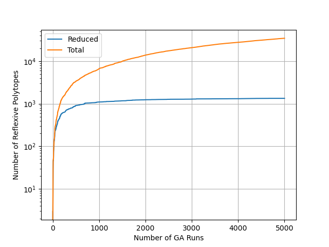
Figure 1: Log plot of total number of generated four-dimensional reflexive polytopes with five vertices against number of genetic algorithm evolutions. The total before and after removing redundancy are shown in orange and blue, respectively.

Next, we are searching for polytopes with a given number, $N_{\text{p},0}$ of lattice points, so we set $w_{3}=0$ and $w_{4}>0$ in the fitness function (6). Specifically, we will be focusing on the cases $N_{\text{p},0}\in\{6,7,8,9,10\}$. The vertex coefficients of such polytopes with a relatively small number of points are likely to be small. Therefore, we reduce the integer range to $x_{a}^{i}\in[-3,4]$ and describe every integer by $\nu=3$ bits. This leads to a reduction of the environment size and a significant improvement in the algorithm’s performance, compared to the previous case. If a polytope has $N_{p,0}$ points, the maximum number of vertices is $N_{\text{v}}=N_{\text{p},0}-1$, where all points are vertices except the origin. Therefore, in searching for polytopes with $N_{\text{p},0}$ points we set the number of generators to $m=N_{\text{p},0}-1$. The results are summarised in Table 1.

# points	# states	$n_{\text{pop}}$	# refl. poly.	# GA runs	states visited
$6$	$\sim 10^{19}$	$400$	$3$	$5$	$\sim 10^{-13}$
$7$	$\sim 10^{22}$	$300$	$25$	$30$	$\sim 10^{-16}$
$8$	$\sim 10^{26}$	$400$	$168$	$60$	$\sim 10^{-19}$
$9$	$\sim 10^{29}$	$300$	$892$	$9378$	$\sim 10^{-20}$
$10$	$\sim 10^{33}$	$350$	$3838$	$9593$	$\sim 10^{-24}$

Table 1: Results for four-dimensional reflexive polytopes with the a small number of lattice points, as in the first column. The size of the environment used for the GA is provided in the second column, the population size in the third column, the fourth column lists the total number of reflexive polytopes for the given number of points (as taken from the Kreuzer–Skarke list) and the fifth column gives the number of GA runs required to find this total. The last column provides an upper bound on the fraction of states visiting during all GA runs.

It is remarkable that all states are found in all cases after a sufficient number of GA runs.

5 Five-dimensional results

In the previous section, we have seen that GAs can generate complete or near-complete lists of reflexive polytopes in two, three, and four dimensions. This is a valuable proof of principle which demonstrates that GAs can successfully identify reflexive polytopes. However, the results are of limited practical use, given the complete classifications in those dimensions. We now turn to reflexive polytopes in five dimensions, the lowest-dimensional case for which a complete classification is not available. The total number of (inequivalent) reflexive polytopes in dimensions $n=1,2,3,4$ is given by $1$, $16$, $4319$, $473,800,776$, respectively. This sequence suggests the number of reflexive polytopes in five dimensions is extremely large and producing a complete catalog is intractable. The partial list of Schöller and Skarke of $185,269,499,015$ weight systems that give rise to “maximal” five-dimensional reflexive polytopes Sch_ller_2019 is the state of the art. The GA, however, is not biased towards generating maximal polytopes, and can be configured to search for polytopes with other properties. In fact, it is likely that the vertices of the largest polytopes are far from the origin, and the GA would struggle to find such cases. For this reasons, we focus on generating polytopes with a small number of points and vertices. In short, while the Schöller–Skarke list consists of maximal polytopes, our GA runs produce small polytopes.

We can compute the normal forms of the polytopes found by the GA with those of the polytopes in the existing list, to confirm that we have indeed found new five-dimensional reflexive polytopes.

5.1 $\bm{N_{\text{v}}=6}$

In analogy with the four-dimensional case, we start by looking at polytopes with the smallest number of vertices, that is, $N_{\text{v}}=6$. We use the integer range $\{-15,\ldots,16\}$ so that every integer is represented by $\nu=5$ bits and the total length of the genotype is $n_{\text{bits}}=150$. Hence, the size of the environment is $2^{150}\simeq 10^{46}$. We have performed $210100$ GA runs, until no new reflexive polytopes were found for $1000$ evolutions, each run with $n_{\text{gen}}=500$ generations and a population size $n_{\text{pop}}=500$. This means a fraction of at most $10^{-36}$ of the environment has been visited. The number of reflexive polytopes against the number of runs found in this way is shown in Figure 2. After removing redundancies, this leads to a total of $77470$ five-dimensional reflexive polytopes with six vertices.

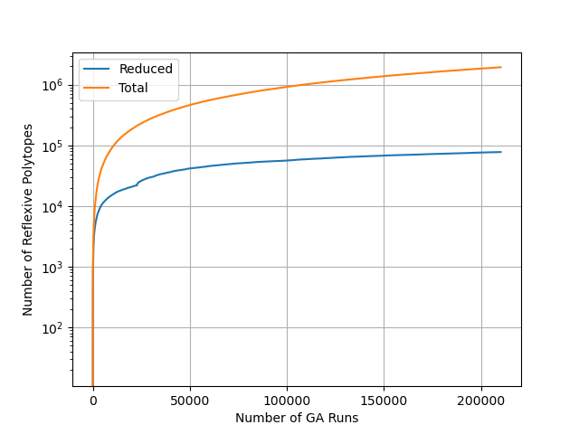
Figure 2: Total number of generated five-dimensional reflexive polytopes with six vertices against number of genetic algorithm evolutions.

Of course we do not know with certainty which fraction of six-vertex polytopes we have found in this way. Just as for the five-vertex search in four dimensions, it is likely some polytopes cannot be found simply because none of their possible vertex matrices fall into the search box defined by our integer range $\{-15,\ldots,16\}$. It is possible to test how much we are missing for this reason by re-running the search with a larger integer range, although we have not attempted this. On the other hand, given the apparent saturation in Figure 2 and in view of the highly successful five-vertex search in four dimensions, it seems likely we have found a large fraction of those polytopes.

5.2 $\bm{N_{\text{p}}=7,8,9,10,11}$

We have also searched for those five-dimensional reflexive polytopes with the lowest number of points, that is, $N_{{\rm p},0}\in\{7,8,9,10,11\}$. This has been done for the range integer range $\{-3,\ldots,4\}$, so that every integer is represented by $\nu=3$ bits, leading the bit strings of length $n_{\text{bits}}=15(N_{{\rm p},0}-1)$. In each case, we perform as many GA runs as necessary until no new polytopes are found for $1000$ evolutions. The results are presented in Table 2.

# points	# states	$n_{\text{pop}}$	# refl. poly.	# GA runs	states visited
$7$	$\sim 10^{28}$	$350$	$9$	$36$	$\sim 10^{-22}$
$8$	$\sim 10^{32}$	$350$	$115$	$1278$	$\sim 10^{-24}$
$9$	$\sim 10^{37}$	$450$	$1385$	$7520$	$\sim 10^{-28}$
$10$	$\sim 10^{41}$	$750$	$12661$	$31857$	$\sim 10^{-31}$
$11$	$\sim 10^{46}$	$650$	$87907$	$67382$	$\sim 10^{-36}$

Table 2: Results for five-dimensional reflexive polytopes with the a small number of lattice points, as in the first column. The size of the environment used for the GA is provided in the second column, the population size in the third column, the fourth column lists the total number of reflexive polytopes found by the GA for the given number of points and the fifth column gives the number of GA runs at which the total list of reflexive polytopes saturates and after which no new reflexive polytopes are found for 1000 runs. The last column provides an upper bound on the fraction of states visiting during all GA runs.

As before, these searches may miss some states, in particular because they fall outside the search box. However, Table 2 certainly provides lower bounds on the number of five-dimensional reflexive polytopes with the lowest number of points and, from the analogous results in the four-dimensional case, we are confident that these bounds are rather strong.

5.3 $\bm{h^{1,1}=1,2}$

It is interesting to ask about CY manifolds with small Hodge numbers and here we focus on cases with small $h^{1,1}$. The Schöller–Skarke list contains $8$ weight systems corresponding to CY hypersurfaces with $h^{1,1}=1$ and $33$ weight systems corresponding to CY hypersurfaces with $h^{1,1}=2$. The maximum number of points of the reflexive polytopes in these lists is $11$. We have scanned the lists of five-dimensional reflexive polytopes obtained from the GA runs described above and have found $15$ polytopes with $h^{1,1}=1$ and $195$ polytopes with $h^{1,1}=2$. By comparing normal forms, we have verrified that these contain all $h^{1,1}=1,2$ polytopes from the Schöller–Skarke list. In addition, there are many new examples, even some with Hodge numbers which are not contained in the Schöller–Skarke list or in the list of four-dimensional CY manifolds realized as complete intersections in products of projective space (CICYs) Gray:2013mja ; cicy4 . Two such examples with a new set of Hodge numbers are given below.

Example 1

A new polytope with $h^{1,1}=1$ is given by the vertex matrix:

$$\left(\begin{array}[]{rrrrrr}-2&1&-1&1&1&0\\ 0&0&1&-1&0&0\\ 1&1&-1&0&0&0\\ 0&-1&-2&2&-1&2\\ -1&2&0&0&0&-1\end{array}\right)~{}.$$ (7)

This polytope has Hodge numbers $h^{1,2}=0$, $h^{1,3}=111$, $h^{2,2}=492$, and Euler number $\chi=720$.

Example 2

A new polytope with $h^{1,1}=2$ is given by the vertex matrix:

$$\left(\begin{array}[]{rrrrrrr}-1&1&0&1&0&0&-1\\ 0&-1&-1&1&1&0&0\\ 1&-3&-1&-1&1&1&3\\ 2&-2&0&-1&-2&1&3\\ -2&2&1&1&0&-1&-2\end{array}\right)~{}.$$ (8)

This polytope has Hodge numbers $h^{1,2}=0$, $h^{1,3}=111$, $h^{2,2}=496$, and Euler number $\chi=726$.

All $15$ polytopes with $h^{1,1}=1$ arise from the datasets with $N_{\text{p}}=7,8$ and no such polytopes are found for $8<N_{\text{p}}\leq 11$. We take this as evidence that the dataset is complete.

Conjecture 5.1

There are precisely $15$ five-dimensional reflexive polytopes that give rise to four complex dimensional Calabi–Yau hypersurfaces with Hodge number $h^{1,1}=1$.

5.4 Targeted searches

To showcase the capability of our GA at generating CY four-folds with specific criteria, we present an example of a targeted search inspired by Berg_2003 . In that paper, the authors consider eleven-dimensional supergravity compactified on CY four-folds with $4$-form flux and provide the conditions necessary to break supersymmetry from $\mathcal{N}=2$ to $\mathcal{N}=1$. In Appendix A they search for CY four-folds with $\chi$ divisible by $\delta\in\{24,224,504\}$ which satisfy the $\mathcal{N}=1$ condition. By searching the Schöller–Skarke list they find eight examples which they present in their Table 1. To facilitate a GA search for such cases, we modify our fitness function to

$$\widetilde{f}(\Delta)=f(\Delta)-w_{5}\sum_{\delta}\chi(\Delta)\mbox{ mod }\delta\;,$$ (9)

where $w_{5}$ is a weight and $\chi(\Delta)$ is the Euler number of $\Delta$. In our search for such polytopes we set the number of generators to be $m=10$ and use the integer coordinate range $[-3,4]$, where each integer is represented by a $\nu=3$ bits. With population size $n_{\text{pop}}=550$ and after $10$ evolutions the GA finds $21$ polytopes that satisfy the index condition and, comparing with Berg_2003 , it turns out all of these are new. One of these is given below.

Example 3

A five-dimensional reflexive polytope giving rise to a four-dimensional CY hypersurface whose Euler number $\chi$ is divisible by $24$, $224$, and $504$ is given by the vertex matrix:

$$\left(\begin{array}[]{rrrrrrr}-1&0&0&-1&-1&0&0\\ 0&1&-3&0&1&-1&0\\ 1&-1&-1&0&-1&1&0\\ 1&-1&1&-1&-1&1&-1\\ -1&1&0&0&1&0&0\end{array}\right)~{}.$$ (10)

This polytope has Hodge numbers $h^{1,1}=4$, $h^{1,2}=1$, $h^{1,3}=325$, $h^{2,2}=1358$, and Euler number $\chi=2016$.

This examples illustrates the possibilities of a targeted GA search. By a suitable modification of the fitness function one can design a dedicated search for CY manifolds with prescribed properties, for example with certain values of the Euler number as above, but also with a given pattern of Hodge numbers, with Chern classes and intersection form satisfying certain constraints or combinations of all of these. This points to a different approach for dealing with large classes of geometries in string theory. Rather than producing complete lists of such geometries (which is not even feasible for the case at hand, that is, five-dimensional reflexive polytopes) the GA can be used to search for geometries with prescribed properties, as required for the intended string compactification.

6 Discussion

In this paper we have shown that genetic algorithms (GAs) can be efficiently used to generate reflexive polytopes in two, three, four, and five dimensions. In two dimensions we have generated the complete set of $16$ reflexive polytopes in just one GA evolution. We have also generated the complete set of reflexive polytopes in three dimensions in $\sim 100000$ evolutions. Due to the large number of reflexive polytopes in four dimensions, we have refrained from generating the complete set in this case. Instead, we have focused on the polytopes with the smallest number $N_{{\rm p},0}$, of lattice points, that is, $6\leq N_{{\rm p},0}\leq 10$. By comparing with the Kreuzer–Skarke classification, we have shown that the GA can find all such polytopes. These results indicate that complete or near-complete classifications of reflexive polytopes can be accomplished with GAs, at least for cases with a small number of lattice points.

This observation is important for the five-dimensional case, where only a partial classification of reflexive polytopes exists. Performing a GA search for $7\leq N_{{\rm p},0}\leq 11$ in five dimensions produces all reflexive polytopes from the partial classification and indeed many more, previously unknown cases. This includes cases which lead to CY four-folds with new sets of Hodge numbers. While the numbers of reflexive polytopes obtained in this way (see Table 2) is unlikely to be the true total there are good indications that they provide strong lower bounds. From these lists, we have also extracted all polytopes with $h^{1,1}=1$. We conjecture that the $15$ cases found constitute the complete list of reflexive polytopes which give rise to CY four-folds with $h^{1,1}=1$.

It is perhaps not desirable, or even feasible, to generate the complete list of reflexive polytopes beyond four dimensions. Instead, we propose an alternative approach, well-suited to the needs of string compactifications, of targeted searches for reflexive polytopes (and their associated CY manifolds) with certain prescribed properties. We have demonstrated that GAs can be used for such targeted searches, by looking for cases with certain prescribed values of the Euler number. This has led to new reflexive polytopes that satisfy the condition for M-theory compactifications on CY four-folds, following Berg_2003 . We expect the same approach will work for other targets, such as a certain desirable pattern of Hodge numbers.

The c code underlying the above results and all data sets are available on GitHub Reflexive_Polytope_Genetic ; githubcGA .

There are many possible directions for future research. In particular, by fine, star, regular triangulation of a (dual) reflexive polytope into simplices, we can construct the CY hypersurface explicitly. This process is also amenable to attack with GAs. Targeted GA searches are another promising avenue. For example, it might be possible to design a targeted search for elliptically or K3 fibered CY four-folds. More ambitiously, one can aim for searches which produce F-theory compactifications with certain desirable properties. It might also be interesting to apply reinforcement learning to the problem of searching for reflexive polytopes and compare its performance to that of GAs. We leave this to future work.

Appendix A Calabi–Yau manifolds from reflexive polytopes

In this section, we briefly review the necessary elements of toric geometry, with the goal of introducing the construction of mirror pairs of Calabi–Yau (CY) manifolds from reflexive polytopes.

Definition A.1

Let $M\cong\mathbb{Z}^{n}$ and $N=\text{Hom}(M,\mathbb{Z})$ be a dual pair of lattices with the pairing $\langle\cdot,\cdot\rangle:N\times M\rightarrow\mathbb{Z}$, and let $M_{\mathbb{Q}}$, $N_{\mathbb{Q}}$ be their rational extensions.

• A polytope $\Delta$ in $M_{\mathbb{Q}}$ is the convex hull of finite number of points in $M_{\mathbb{Q}}$.

• $\Delta$ is called a lattice polytope if all its vertices lie in $M$.

• The dual or polar polytope of $\Delta$ is defined as

  $$\Delta^{*}=\{n\in N_{\mathbb{Q}}|\langle n,m\rangle\geq-1\ \forall\,m\in\Delta\}~{}.$$ (11)

• A face $\theta$ of $\Delta$ is defined as

  $$\theta=\{m\in\Delta|\langle n,m\rangle=r\}~{},$$ (12)

  for some $n\in N_{\mathbb{Q}}$ and $r\in\mathbb{R}$.

Given an $n$-dimensional lattice polytope $\Delta$, one can construct a compact toric variety $X_{\Delta}$ of complex dimension $n$. In short, one constructs the normal fan $\Sigma_{\Delta}$ as follows: for a face $\theta$ of $\Delta$, let $\sigma_{\theta}\subset N_{\mathbb{R}}$ be the dual of the cone:

$$\sigma_{\theta}^{\vee}:=\{\lambda(u-u^{\prime})|u\in\Delta,u^{\prime}\in\theta,\lambda\geq 0\}\subset M_{\mathbb{R}}~{}.$$ (13)

Then the normal fan is given as $\Sigma_{\Delta}:=\{\sigma_{\theta}\}$ for all faces $\theta$ of $\Delta$. From the normal fan, the construction of the compact toric variety $X_{\Delta}$ follows the usual procedure fulton , where each cone gives rise to an affine toric variety and one glues these patches together.

Definition A.2

A polytope is said to satisfy the interior point (IP) property when it contains only one interior point taken to be the origin. Let $\Delta\subset M$ be a lattice polytope satisfying the IP property, then $\Delta$ is called reflexive if its dual $\Delta^{*}\subset N$ is also a lattice polytope satisfying the IP property.

We recall that a CY $n$-fold $\mathcal{M}$ is an $n$ complex dimensional space that is a compact Kähler manifold and has a vanishing first real Chern class. Calabi conjectured and Yau proved that such a geometry admits a unique Ricci-flat metric in each Kähler class.

The connection between CY manifolds and reflexive polytopes is the following. Let $\Delta\subset M$ be an $n$-dimensional reflexive polytope and $X_{\Delta}$ the corresponding $n$ complex dimensional toric variety. Then it follows that the zero locus of a generic section of the anticanonical bundle $-K_{X}$ is a CY variety $\mathcal{M}$ of dimension $n-1$ which can be resolved into a CY orbifold with at most terminal singularities. The mirror CY $\mathcal{W}$ is similarly obtained from the polar dual. (Because of the IP property, it turns out that $(\Delta^{*})^{*}=\Delta$.) See Altman:2014bfa ; Demirtas:2022hqf for explicit constructions of CY manifolds from reflexive polytopes.

Appendix B Normal form

There are two sources of redundancy when defining a reflexive polytope $\Delta$ in $n$ dimensions by its $n\times N_{\text{v}}$ vertex matrix $V$, whose columns are the $N_{\text{v}}$ vertices. First of all, one permute the vertices, leading to an $S_{N_{\text{v}}}$ symmetry which permutes the columns of $V$. Secondly, one can perform a coordinate transformation on the $n$-dimensional lattice by acting on $V$ with a ${\rm GL}(n,\mathbb{Z})$ matrix from the left. Altogether, this amounts to a transformation of the vertex matrix as in Eq. (1).

In order to remove the redundancy in the list of polytopes, we compare their normal forms. This is the approach that was used by Kreuzer and Skarke in constructing the complete classification of three- and four-dimensional reflexive polytopes kreuzer1998classification ; kreuzer2000complete and is included in the PALP software package Kreuzer_2004 . If two polytopes $\Delta_{1}$ and $\Delta_{2}$ have the same normal form, then they are equivalent, in the sense that they are isomorphic with respect to a lattice automorphism. A detailed description of the how one computes the normal form is given in grinis2013normal . We shall give a short description here.

Let $M$ be a $n$-dimensional lattice and $\Delta\subset M_{\mathbb{Q}}$ a $n$-dimensional lattice polytope with $N_{\text{v}}$ vertices, $N_{\text{f}}=|F(\Delta)|$ facets and vertex matrix $V$. We also define the supporting hyperplanes of $\Delta$, associated to the facets $\varphi_{i}\in F(\Delta)$, as the set of all vectors $v$ satisfying $\langle w_{i},v\rangle=-c_{i}$, where $(w_{i},c_{i})\in M^{*}\times\mathbb{Z}$. The algorithm to compute the normal form is then as follows.

1. Compute the $N_{\text{f}}\times N_{\text{v}}$ vertex-facet pairing matrix $PM$:

   $$PM_{ij}:=\langle w_{i},v_{j}\rangle+c_{i}~{}.$$ (14)

2. Order the pairing matrix $PM$ lexicographically to get the maximal matrix $PM^{\text{max}}$.

3. Further rearrange the columns of $PM^{\text{max}}$ to get $M$ by the following:

   $$M\leftarrow PM^{\text{max}}$$

   $$\textbf{for }i=1\textbf{ to }N_{\text{v}}\textbf{ do}$$

   $$\hskip 28.45274ptk\leftarrow i$$

   $$\hskip 28.45274pt\textbf{for }j=i+1\textbf{ to }N_{\text{v}}\textbf{ do}$$

   $$\hskip 28.45274pt\hskip 28.45274pt\textbf{if }c_{M}(j)<c_{M}(k)\vee(c_{M}(j)=c_{M}(k)\wedge s_{M}(j)<s_{M}(k))\textbf{ then}$$

   $$\hskip 28.45274pt\hskip 28.45274pt\hskip 28.45274ptk\leftarrow j$$

   end if

   end for

   $$\hskip 28.45274ptM\leftarrow\text{SwapColumn}(M,i,k)$$

   end for

   where $c_{M}(j):=\text{max}(M_{ij}|1\leq i\leq N_{\text{f}})$ and $s_{M}(j):=\sum_{i=1}^{N_{\text{f}}}M_{ij}$, where $1\leq j\leq N_{\text{v}}$.

4. Let $\sigma_{\text{max}}$ denote the associated element of $S_{N_{\text{f}}}\times S_{N_{\text{v}}}$ that transforms $PM$ into $M$. Order the columns of $V$ according to the restriction of $\sigma_{\text{max}}$ to $S_{N_{\text{v}}}$ to get the maximal vertex matrix $V^{\text{max}}$. This removes the permutation degeneracy.

5. Compute the row style Hermite normal form of $V^{\text{max}}$ to obtain the normal form $NF$. This step removes the $GL(n,\mathbb{Z})$ degeneracy.

Example 4

To illustrate the above algorithm, we present an example in three dimensions. Let $\Delta$ be a lattice polytope defined by the vertex matrix:

$$V=\left(\begin{array}[]{rrrrrrrrrrrr}3&1&4&0&2&3&3&-3&1&-3&0&-3\\ -3&2&0&-1&1&2&1&2&2&-2&-3&2\\ -3&4&1&4&4&-1&-2&-1&-3&2&0&2\end{array}\right)\;.$$ (15)

Computing the vertex-facet pairing matrix we get

$$PM=\setcounter{MaxMatrixCols}{12}\begin{pmatrix}2&2&0&0&0&5&5&11&9&4&2&8\\ 7&0&3&0&0&5&6&5&7&2&4&2\\ 0&70&51&59&73&30&18&0&0&22&15&30\\ 3&7&3&11&7&0&0&6&0&13&9&9\\ 0&56&21&67&53&6&0&36&0&68&39&60\\ 5&0&2&3&1&0&1&0&0&4&5&0\\ 0&10&8&6&10&7&5&1&3&0&0&4\\ 3&6&5&0&4&11&10&11&13&0&0&8\\ 0&5&1&0&2&8&7&14&12&3&0&11\\ 6&4&7&3&5&6&6&0&4&0&3&0\\ 27&2&17&0&4&21&24&9&23&0&12&0\\ 53&0&29&0&4&36&43&18&42&4&26&0\end{pmatrix}.$$ (16)

Ordering $PM$ lexicographically we get the following maximal matrix:

$$PM^{\text{max}}=\setcounter{MaxMatrixCols}{12}\begin{pmatrix}217&212&173&138&135&96&72&44&3&0&0&0\\ 73&70&51&30&59&18&30&0&15&22&0&0\\ 53&56&21&6&67&0&60&0&39&69&36&0\\ 37&49&0&3&65&0&93&21&51&97&81&0\\ 12&44&0&73&0&65&118&121&6&42&151&0\\ 10&13&0&0&20&0&27&6&18&31&24&3\\ 10&10&8&7&6&5&4&3&0&0&1&0\\ 7&7&3&0&11&0&9&0&9&13&6&3\\ 5&4&7&6&3&6&0&4&3&0&0&6\\ 4&6&5&11&0&10&8&13&0&0&11&3\\ 4&2&17&21&0&24&0&23&12&0&9&27\\ 4&0&29&36&0&43&0&42&26&4&18&53\end{pmatrix},$$ (17)

corresponding to the row and column permutations $(12,2,4,14,17,13,6,3,9,7,10,11)$ and $(4,1,2,5,3,6,11,8,10,9,7,0)$ respectively. Further ordering the columns by the procedure described in Step 3 above we get

$$M=\setcounter{MaxMatrixCols}{12}\begin{pmatrix}217&0&72&0&0&3&138&96&44&173&212&135\\ 73&0&30&22&0&15&30&18&0&51&70&59\\ 53&36&60&69&0&39&6&0&0&21&56&67\\ 37&81&93&97&0&51&3&0&21&0&49&65\\ 12&151&118&42&0&6&73&65&121&0&44&0\\ 10&24&27&31&3&18&0&0&6&0&13&20\\ 10&1&4&0&0&0&7&5&3&8&10&6\\ 7&6&9&13&3&9&0&0&0&3&7&11\\ 5&0&0&0&6&3&6&6&4&7&4&3\\ 4&11&8&0&3&0&11&10&13&5&6&0\\ 4&9&0&0&27&12&21&24&23&17&2&0\\ 4&18&0&4&53&26&36&43&42&29&0&0\\ \end{pmatrix},$$ (18)

corresponding to the column permutation $(0,10,6,9,11,8,3,5,7,2,1,4)$. Ordering the columns in $V$ correspondingly we get

$$V^{\text{max}}=\left(\begin{array}[]{rrrrrrrrrrrr}3&0&3&-3&-3&1&0&3&-3&4&1&2\\ -3&-3&1&-2&2&2&-1&2&2&0&2&1\\ -3&0&-2&2&2&-3&4&-1&1&1&4&4\\ \end{array}\right)\;.$$ (19)

Finally, computing the row style Hermite normal form of $V^{\text{max}}$ we arrive at the following normal form:

$$NF=\left(\begin{array}[]{rrrrrrrrrrrr}3&0&0&0&0&7&-12&-3&9&-11&-14&-16\\ 0&3&0&1&-3&-11&17&3&-15&16&17&21\\ 0&0&1&-1&-1&-2&4&2&-4&5&5&6\end{array}\right)\;.$$ (20)

References

- (1) P. Candelas, G. T. Horowitz, A. Strominger, E. Witten, Vacuum configurations for superstrings, Nucl. Phys. B 258 (1985) 46–74. doi:10.1016/0550-3213(85)90602-9.
- (2) T. Hubsch, Calabi-Yau manifolds: A Bestiary for physicists, World Scientific, Singapore, 1994.
- (3) Y.-H. He, The Calabi–Yau Landscape: From Geometry, to Physics, to Machine Learning, Lecture Notes in Mathematics, 2021. arXiv:1812.02893, doi:10.1007/978-3-030-77562-9.
- (4) J. Bao, Y.-H. He, E. Hirst, S. Pietromonaco, Lectures on the Calabi-Yau Landscape (1 2020). arXiv:2001.01212.
- (5) V. V. Batyrev, Dual polyhedra and mirror symmetry for calabi-yau hypersurfaces in toric varieties (1993). arXiv:alg-geom/9310003.
- (6) V. V. Batyrev, L. A. Borisov, On calabi-yau complete intersections in toric varieties (1994). arXiv:alg-geom/9412017.
- (7) M. Kreuzer, H. Skarke, On the classification of reflexive polyhedra, Communications in Mathematical Physics 185 (2) (1997) 495–508. doi:10.1007/s002200050100.
- (8) M. Kreuzer, H. Skarke, Classification of reflexive polyhedra in three dimensions (1998). arXiv:hep-th/9805190.
- (9) H. Skarke, Weight systems for toric calabi-yau varieties and reflexivity of newton polyhedra, Modern Physics Letters A 11 (20) (1996) 1637–1652. doi:10.1142/s0217732396001636.
- (10) M. Kreuzer, H. Skarke, Complete classification of reflexive polyhedra in four dimensions (2000). arXiv:hep-th/0002240.
- (11) F. Schöller, H. Skarke, All weight systems for calabi–yau fourfolds from reflexive polyhedra, Communications in Mathematical Physics 372 (2) (2019) 657–678. doi:10.1007/s00220-019-03331-9.
-
(12)
M. Kreuzer, H. Skarke,
Calabi-yau data.
URL https://hep.itp.tuwien.ac.at/~kreuzer/CY/ - (13) J. Bao, Y.-H. He, E. Hirst, J. Hofscheier, A. Kasprzyk, S. Majumder, Polytopes and machine learning (2021). arXiv:2109.09602.
- (14) D. S. Berman, Y.-H. He, E. Hirst, Machine learning Calabi-Yau hypersurfaces, Phys. Rev. D 105 (6) (2022) 066002. arXiv:2112.06350, doi:10.1103/PhysRevD.105.066002.
- (15) P. Berglund, B. Campbell, V. Jejjala, Machine Learning Kreuzer-Skarke Calabi-Yau Threefolds (12 2021). arXiv:2112.09117.
- (16) S. A. Abel, J. Rizos, Genetic algorithms and the search for viable string vacua, Journal of High Energy Physics 10 (2014) 1029–8479. doi:10.1007/JHEP08(2014)010.
- (17) S. Abel, A. Constantin, T. R. Harvey, A. Lukas, String model building, reinforcement learning and genetic algorithms (2021). arXiv:2111.07333.
- (18) S. A. Abel, A. Constantin, T. R. Harvey, A. Lukas, Cosmic inflation and genetic algorithms, Fortschritte der Physik 71 (1) (2022) 2200161. doi:10.1002/prop.202200161.
-
(19)
B. I. U. Nødland, Generating
refelexive polytopes via sequence modeling (2022).
URL https://mathai2022.github.io/papers/3.pdf -
(20)
S. Abel, A. Constantin, T. R. Harvey, A. Lukas, L. A. Nutricati,
A realisation of genetic
algorithms in c, Tech. rep. (April 2023).
URL https://github.com/harveyThomas4692/GA-C -
(21)
P. Berglund, Y.-H. He, E. Heyes, E. Hirst, V. Jejjala, A. Lukas,
Reflexive Polytope
Genetic Algorithm.
URL https://github.com/elliheyes/Polytope-Generation - (22) J. C. Lagarias, G. M. Ziegler, Bounds for lattice polytopes containing a fixed number of interior points in a sublattice, Canadian Journal of Mathematics 43 (5) (1991) 1022–1035. doi:10.4153/CJM-1991-058-4.
- (23) C. Darwin, On the Origin of Species by Means of Natural Selection, or the Preservation of Favored Races in the Struggle for Life, Murray, London, 1859.
- (24) A. M. Turing, Computing machinery and intelligence, Mind 59 (236) (1950) 433.
- (25) N. A. Barricelli, Esempi numerici di processi di evoluzione, Methodos 6 (21-22) (1954) 45–68.
- (26) J. Holland, Adaptation in natural and artificial systems (1992).
- (27) D. E. Goldberg, Genetic Algorithms in Search, Optimization and Machine Learning, Addison-Wesley, 1989.
- (28) J. Holland, The royal road for genetic algorithms: Fitness landscapes and ga performance, in: Toward a Practice of Autonomous Systems: proceedings of the first European conference on Artificial Life, F. J. Varela and P. Bourgine, eds. (1992).
- (29) C. Reeves, J. Rowe, Genetic Algorithms: Principles and Perspectives, Springer, 2002.
- (30) P. Charbonneau, An introduction to genetic algorithms for numerical optimization, Tech. Rep. Tech. Rep. TN-450+IA, National Center for Atmospheric Research (2002).
- (31) R. Haupt, S. Haupt, Practical genetic algorithms, 2nd Edition, Wiley, 2004.
- (32) D. Michalewicz, How to Solve It: Modern Heuristics, 2nd Edition, Springer, 2004.
- (33) M. Kreuzer, H. Skarke, PALP: A package for analysing lattice polytopes with applications to toric geometry, Computer Physics Communications 157 (1) (2004) 87–106. doi:10.1016/s0010-4655(03)00491-0.
- (34) J. Gray, A. S. Haupt, A. Lukas, All Complete Intersection Calabi-Yau Four-Folds, JHEP 07 (2013) 070. doi:10.1007/JHEP07(2013)070.
-
(35)
J. Gray, A. S. Haupt, A. Lukas,
Complete
intersection Calabi-Yau four-folds.
URL https://www-thphys.physics.ox.ac.uk/projects/CalabiYau/Cicy4folds/index.html - (36) M. Berg, M. Haack, H. Samtleben, Calabi-yau fourfolds with flux and supersymmetry breaking, Journal of High Energy Physics 2003 (04) (2003) 046–046. doi:10.1088/1126-6708/2003/04/046.
-
(37)
W. Fulton, Introduction to
Toric Varieties. (AM-131), Princeton University Press, 1993.
URL https://www.jstor.org/stable/j.ctt1b7x7vc - (38) R. Altman, J. Gray, Y.-H. He, V. Jejjala, B. D. Nelson, A Calabi-Yau Database: Threefolds Constructed from the Kreuzer-Skarke List, JHEP 02 (2015) 158. doi:10.1007/JHEP02(2015)158.
- (39) M. Demirtas, A. Rios-Tascon, L. McAllister, CYTools: A Software Package for Analyzing Calabi-Yau Manifolds (11 2022). arXiv:2211.03823.
- (40) R. Grinis, A. Kasprzyk, Normal forms of convex lattice polytopes (2013). arXiv:1301.6641.