Neural Algorithmic Reasoning for Combinatorial Optimisation

Abstract

Solving NP-hard/complete combinatorial problems with neural networks is a challenging research area that aims to surpass classical approximate algorithms. The long-term objective is to outperform hand-designed heuristics for NP-hard/complete problems by learning to generate superior solutions solely from training data. Current neural-based methods for solving CO problems often overlook the inherent “algorithmic” nature of the problems. In contrast, heuristics designed for CO problems, e.g. TSP, frequently leverage well-established algorithms, such as those for finding the minimum spanning tree. In this paper, we propose leveraging recent advancements in neural algorithmic reasoning to improve the learning of CO problems. Specifically, we suggest pre-training our neural model on relevant algorithms before training it on CO instances. Our results demonstrate that by using this learning setup, we achieve superior performance compared to non-algorithmically informed deep learning models.

1 Introduction

Combinatorial problems have immense practical applications and are the backbone of modern industries. For example, the Travelling Salesman Problem (TSP) has applications as diverse as logistics Baniasadi et al. [4], route optimisation [53], scheduling to genomics [42] and systems biology [28]. The problem has been studied by both theoretical computer scientists [3, 30] and the ML community [50, 34, 29] from different perspectives. The former targets the development of hand-engineered approximate algorithms, which trade-off optimality for computational complexity, whereas the latter’s ultimate objective is to learn such algorithms instead of manually designing them, i.e. Neural Combinatorial Optimisation (NCO). Hence, learning to solve such a problem and pushing the performance beyond that of hand-crafted heuristics, such as the Christofides’ [8] algorithm, is a fascinating goal that can have a direct impact on the aforementioned industrial fields.

Existing works attempt to learn solutions for CO problems by either supervised learning [29] or reinforcement learning [34], exploiting standard deep learning methods. Although many combinatorial problems have natural “algorithmic” solutions [8, 6], leveraging algorithmic knowledge has never been explored in prior work.

For example, the Christofides’ algorithm follows several steps to construct a solution for the TSP. First, it computes the minimum spanning tree (MST) and subsequently applies a matching algorithm to it. In light of this observation, we argue that knowledge of algorithms may be useful also when addressing combinatorial problems through the use of neural networks. Our hypothesis is that a neural network that possesses knowledge of, say, the minimum spanning tree, might be able to generalise better when learning to solve the TSP. In this context, recent advancements in Neural Algorithmic Reasoning (NAR) [45] neural networks have been shown to effectively learn and reproduce the execution of classical algorithms [45], such as the Prim’s algorithm [39]. Moreover, current “neural algorithmic reasoners” can learn multiple algorithms at once, showing positive transfer knowledge across them. This yields to better results compared to learning a single algorithm in isolation.

Motivated by this, in this paper, we explore the applicability of NAR in the context of NCO. So far, most of the prior work in neural algorithmic reasoning focuses on learning algorithms and solving problems within the class of complexity of problems solvable in polynomial time, i.e. P. In our settings, we aim to solve challenging combinatorial problems, e.g., TSP, which are known to be NP-complete/hard. Hence, we try to transfer algorithmic knowledge from algorithms and problems that are in P to NP-complete/hard problems. To the best of our knowledge, we are the first to explore transferring from algorithmic reasoning to NP-complete/hard combinatorial optimisation problems.

In general, the contributions of our work can be summarised as follows: (i) we show that algorithms are a good inductive bias in the context of NCO and leads to good OOD generalisation w.r.t. algorithm-agnostic baselines; (ii) we investigate and study how different NAR transfer learning settings perform when applied on the P$\rightarrow$NP scenario. Interestingly, the best setting is pre-train + finetune – a method that was previously thought inferior in NAR; (iii) we highlight shortcomings of current neural algorithmic reasoners, opening up new potential areas for research.

2 Related work

Neural Combinatorial Optimisation (NCO) is a long-standing research area that aims to exploit the predictive power of deep neural networks to help solve CO problems. Pioneering work from Hopfield and Tank [26] dates back to the 1980s, where the authors designed a specialised loss function to train a rudimentary neural network to solve instances of TSP. Building from there, practitioners have come up with increasingly complex models to solve CO problems, starting from Self-Organising Maps (SOMs) until modern deep learning architectures. The Pointer Networks (Ptr-Nets) [50] represent the first attempt to solve a CO task, namely the TSP, with a pure deep learning approach. Ptr-Nets are sequence-to-sequence recurrent models that process a sequence of 2D geometrical points, e.g. coordinates of TSPs, and “translate” them to a sequence of nodes to be visited, i.e. a tour $\pi$. The original model was trained in a supervised way, even though some different training setups have been explored by later works, such as actor-critic reinforcement learning [5] and REINFORCE [12]. However, the community quickly realised the benefit of using structure-aware learning models, such as Graph Neural Networks (GNNs). Many CO problems, in fact, have natural representations as graphs rather than sequences of points in geometrical spaces (see section 3, TSP paragraph). In particular, Kool et al. [34] and Joshi et al. [29] developed a similar encoder-decoder to Ptr-Nets but treat the input as a graph, incorporating Graph Attention Network (GAT) [49] style updates in their respective architectures. However, the entirety of the proposed approaches in NCO treat the problem as a “standard” predictive task, without taking into account that algorithms play an important role in classical computer science heuristics, e.g. Christofides’ algorithm for TSPs. Differently from all prior works, we incorporate algorithmic reasoning knowledge in our learnt predictor, i.e. a Message-Passing Neural Network (MPNN), by leveraging neural algorithmic reasoning [45].

As introduced in section 3, Neural Algorithmic Reasoning (NAR) involves developing neural models and learning setups to facilitate the encoding of algorithms directly in models’ weights. Starting from some early work [47] that aimed to demonstrate the applicability of GNNs to reproduce classical algorithm steps, the community has then applied these concepts to a variety of domains. Deac et al. [11] successfully trained an algorithmic reasoner to planning problems, by reproducing steps of Bellman optimality equation in a reinforcement learning setting. Xhonneux et al. [51] studied different ways of transferring algorithmic knowledge between algorithms. In particular, they train algorithmic reasoners on a set of algorithms and study the effect of: (i) training on all algorithms simultaneously (multi-task learning); (ii) pre-train on a subset of algorithms and finetune on others; (iii) freeze some parameters of the pre-trained network and learn the remaining; (iv) utilise multiple processors, one of which is frozen. In our work, we experimented with transferring algorithmic knowledge by using and extending these setups. Numeroso et al. [38] train an algorithmic reasoner to solve MaxFlow/MinCut by exploiting the duality of the two optimisation problems. However, the combinatorial problem therein is in P. Differently from them, we try to generalise and transfer algorithmic knowledge from problems that are in P, i.e. shortest path and minimum spanning tree, to harder problems such as the TSP, which is known to be NP-hard.

3 Background

Graph Neural Networks

Graph Neural Networks [2], are a type of deep neural networks designed to operate within a structured input domain, i.e. graphs, by relying on a local context diffusion mechanism. Specifically, let $G=(V,E)$ be a graph with $V$ and $E$ being respectively the set of nodes and edges. Then, GNNs process graphs by propagating information at a node-level, following a message-passing algorithm as follows:

$${\bm{h}}^{(\ell+1)}_{v}=\phi^{(\ell+1)}\big{(}{\bm{h}}^{(\ell)}_{v},\Psi(\{\psi^{(\ell+1)}({\bm{h}}^{(\ell)}_{u})\mid u\in\mathcal{N}(v)\})\big{)}$$ (1)

where $\phi$ and $\psi$ are parameterised transformations, ${\bm{h}}^{(\ell)}_{v}$ is the node representation at layer/iteration $\ell$, with ${\bm{h}}^{(0)}_{v}={\bm{x}}_{v}$ where ${\bm{x}}_{v}$ is a vector of initial features. Function $\Psi$ aggregates the information flowing to node $v$ from its neighbourhood $\mathcal{N}(v)$, and is chosen to be a permutation-invariant function, i.e. a different ordering does not change the final output.

Neural execution of algorithms

Neural Algorithmic Reasoning (NAR) [45] is a developing research area that seeks to build algorithmically-inspired neural networks. In classical algorithms such as Bellman-Ford [41, 17] and Prim [39], solutions are typically constructed through a series of iterations. When executing algorithm $A$ on input ${\bm{x}}$, it produces an output $A({\bm{x}})$ and defines a trajectory of intermediate steps $A_{t}({\bm{x}})$. Unlike traditional machine learning tasks that focus solely on learning an input-output mapping function $f:X\rightarrow A(X)$, NAR aims to impose constraints on the hidden dynamics of neural models to replicate algorithmic behaviours. This is commonly achieved by incorporating supervision on ${A_{t}({\bm{x}})}$ [47] in addition to any supervision on $A({\bm{x}})$.

The encode-process-decode architecture [23] is considered the preferred choice when implementing NAR models [45]. The architecture is a composition of three learnable components $net=g\circ p\circ f$, where $f$ and $g$ are encoding and decoding functions (usually as simple as linear transformations), and $p$ is a suitable neural architecture called processor that mimics the execution rollout of $A$. Typically, we choose $p$ to be the only part of the network having non-linearities to ensure the majority of the architecture’s expressiveness lies within the processor. Furthermore, as shown in Ibarz et al. [27], we are also able to learn multiple algorithms (both graph and non-graph) at once, by having separate $f_{A}$ and $g_{A}$ per an algorithm $A$, and sharing the processor $p$ across all algorithms.

A fundamental objective of NAR is to achieve robust out-of-distribution (OOD) generalisation. Typically, models are trained and validated on “small” graphs (e.g., up to 20 nodes) and tested on larger graphs. This is inspired by classical algorithms’ size-invariance, where correctness of the solution is maintained irrespective of the input size. The rationale behind testing on larger graphs is to assess whether the reasoner has truly captured the algorithm’s behaviour and can extrapolate well beyond the training data, and past the easily exploitable shortcuts in it. Evaluating models on OOD data reveals their ability to generalize and provide accurate solutions in diverse scenarios.

CLRS-30

The CLRS-30 benchmark [48], or CLRS-30, comprises 30 iconic algorithms from the Introduction to Algorithms textbook [9]. The benchmark covers diverse algorithm types, including string algorithms, searching, dynamic programming, and graph algorithms. All data instances in the CLRS-30 benchmark are represented as graphs and are annotated with input, output and hint features and an associated position. Denote the dimensionality of a feature as $F$ and $|V|$ as $N$. Input/output node features have the shape $N\times F$, edge features – $N\times N\times F$, graph features – only $F$. Hints encapsulate time series data of algorithm states. Like inputs/outputs, they include a temporal dimension which also indicates the duration of execution. All features fall into 5 types: scalar, categorical, mask (0/1 value), mask_one (only a single position can be 1), and pointer. Each feature type has an associated loss to be used when training the neural network [cf. 48].

Travelling Salesman Problem

A TSP instance is a complete undirected weighted graph $G=(V,E,w)$. A valid solution for a TSP is a tour $\pi=v_{0}v_{1}\dots v_{|V|}$, wherein $\pi_{0:|V|}$ is a permutation of the $n$ nodes – the node visiting order before returning to the starting node. Among all correct solutions, we usually seek the one minimising the total cost of the tour $c^{*}=\min_{\pi}\sum^{|V|-1}_{i=0}{w_{\pi_{i}\pi_{i+1}}}$.

Vertex K-center

The vertex k-center problem (VKC) [22] is defined as follows: given an undirected weighted graph $G=(V,E,w)$ and a positive integer $k$, find a subset $C\subset V$ where $\lvert C\rvert\leq k$ in order to minimize $o=\max_{v\in V}{w(v,C)}$. In this context, $w(v,C)$ denotes the distance from vertex $v$ to its nearest center in subset $C$. In the original formulation, the problem involves a complete graph and a metric function $w$. To introduce some diversity compared to TSP, we consider (not necessarily fully) connected graphs and necessitate the network to compute the shortest distances between nodes.

4 Neural Algorithmic Reasoning for Combinatorial Optimisation

4.1 Selection of relevant algorithms

In our algorithm selection for pre-training, we prioritize specific subtask-solving algorithms within the target combinatorial optimization problem, like Prim’s algorithm for TSP or Find-Min for VKC. We also consider algorithms that monitor properties (e.g., shortest path) or belong to related classes (e.g., greedy algorithms). Exclusion of algorithms is also vital. We omit algorithms that the base reasoner struggles with (e.g., Floyd-Warshall for VKC, see Table 2) or are resource-intensive (cf. Appendix A) due to their CLRS-30 representation. The final choice is Bellman-Ford and MST-Prim for TSP and Bellman-Ford, min finding, activity selection [19] and task scheduling [35] for VKC. Appendix B provides deeper insights into our algorithm selection process.

4.2 Choice of GNN architecture

The rationale behind selecting our GNN architecture stemmed from the necessity of being able to learn to perform algorithms, in particular shortest path, MST-Prim and Graham Scan. Consequently, we intentionally avoided utilizing architectures such as GCN/GAT [33, 49] which are known to perform poorly in algorithmic reasoning [47] or Pointer Networks [50] which do not incorporate graph structure information. A further reason to avoid standard graph neural TSP architectures is that they usually have fixed depth, while algorithmic reasoning architectures are recurrent.

Despite narrowing down our potential architectures, there have been several impactful architectures in the last few years. Testing each and every possible architecture requires computational resources outside of our reach. In order to choose an appropriate architecture, we focused on several key properties the network should possess: accuracy in graph algorithms and particular Bellman-Ford and MST-Prim, scalability and suitability for TSP. The first requirement has led us to exclude the recently proposed 2-WL architecture by Mahdavi et al. [36]. Lastly, Pointer Graph Networks [46] are unusable for our purpose due to the nature of TSP. Persistent Message Passing [44] is also inappropriate as it targets fundamentally different type of problems.

Based on the above analysis our final choice for a neural algorithmic reasoner is an MPNN architecture with graph features and a gating mechanism as in Ibarz et al. [27]:

$$\mathbf{z}_{i}^{(t)}=\mathbf{u}_{i}^{(t-1)}\|\mathbf{h}_{i}^{(t-1)}\qquad \mathbf{m}_{i}^{(t)}=\max_{1\leq j\leq n}f_{m}\left(\mathbf{z}_{i}^{(t)},\mathbf{z}_{j}^{(t)},\mathbf{e}_{ij}^{(t)}\right)\qquad\mathbf{\hat{h}}_{i}^{(t)}=f_{r}\left(\mathbf{z}_{i}^{(t)},\mathbf{m}_{i}^{(t)}\right)$$

$$\mathbf{g}_{i}^{(t)}=f_{g}(\mathbf{z}_{i}^{(t)},\mathbf{m}_{i}^{(t)})\qquad \mathbf{h}_{i}^{(t)}=\mathbf{g}_{i}^{(t)}\odot\mathbf{\hat{h}}_{i}^{(t)}+(1-\mathbf{g}_{i}^{(t)})\odot\mathbf{\hat{h}}_{i}^{(t)}$$

where $\mathbf{u}_{i}^{(t)}$ are node input/hint features at timestep $t$, ${\bm{h}}_{i}^{(t)}$ is the latent state of node $i$ at timestep $t$ (with ${\bm{h}}_{i}^{(0)}=\mathbf{0}$), $\|$ denotes concatenation and $\odot$ denotes elementwise multiplication. Further, $f_{m}$ is a message function, and $f_{g}$ and $f_{r}$ are gating-related functions of the model. Function $f_{m}$ is parametrised as an MLP, while $f_{g}$ and $f_{r}$ are linear projection layers. Inspired by the architecture of Joshi et al. [29] we also explored having edge hidden states. The state is updated similar to ${\bm{h}}_{i}^{(t)}$ and is used in the message computation: $f_{m}\left(\mathbf{z}_{i}^{(t)},\mathbf{z}_{j}^{(t)},\mathbf{e}_{ij}^{(t)},{\bm{h}}_{ij}^{(t)}\right)$.

4.3 Algorithmic knowledge integration

None of the algorithmic reasoning papers we surveyed experimented with NP-hard problems like TSP. Thus, we decided to test a variety of ways to expose our model to algorithmic knowledge, including those that have previously shown inferior performance [51]. Denote a base task $\mathcal{B}$, from which we want to transfer, and a target task $\mathcal{T}$, which we want to infuse with the knowledge of $\mathcal{B}$. We explored the following integration strategies:

• Pre-train and freeze (PF) – this is the most common setting used when ${\mathcal{B}}$ is an abstract algorithm and ${\mathcal{T}}$ is a real-world task [10, 38, 45]. It consists of pre-training a model on a concrete task (e.g. MST) and copying the processor parameters into the real-world architecture’s processor and freezing them so they cannot be changed.

• Pre-train and fine-tune (PFT) – in the approach above the processor weights are frozen. We hypothesise this may not be suitable for our P to NP-hard transfer, so we provide results using the same transfer learning technique as above but allowing weights to be optimised.

• 2-processor transfer (2PROC) [51] – this technique is a combination of the aforementioned two. When transferring from ${\mathcal{B}}$ to ${\mathcal{T}}$ we use 2 processors: one initialised with the pre-trained parameters and kept frozen and another randomly initialised and fine-tuned.

• Multi-task learning (MTL) – this is a setting where the transfer from ${\mathcal{B}}$ to ${\mathcal{T}}$ is performed implicitly by training ${\mathcal{B}}$ and ${\mathcal{T}}$ together but sharing the same processor. This technique gave the best results in Xhonneux et al. [51] and was also used when training with dual algorithms in Numeroso et al. [38].

5 Evaluation

5.1 Data generation & hyperparameter setup

NAR

For our NAR training set we generated 10000 samples for each algorithm. For pre-training the NAR model for the TSP task we generated each of our graphs by sampling points in 2D space (unit square) and setting the edge weights of the graph equal to the Euclidean distance between nodes. Eventually, graphs are all fully-connected. For VKC, we sample Erdős–Rényi [15] graphs with $p=0.5$, excluding graphs that are disconnected. As it has been shown that varying graph sizes leads to stronger reasoners [36, 27], the size of each graph was uniformly chosen from $[8,16]$. For generating the ground-truth targets and trajectories, we employed the official code for the CLRS-30 benchmark. Although we picked our reasoner based on the best validation score we also built a test set in order to evaluate the capability of our reasoners to generalise. Both validation and test sets comprehend 100 graphs per algorithm, but graph sizes in the validation dataset are fixed at 16, while graphs in the test dataset are of size fixed at 64.

TSP

To train our CO models, we adopted the representation format of CLRS-30 (cf. section 3). As input features for TSP we picked node mask features representing the starting node of the tour and edge scalar features for the distance between nodes. Node coordinates were replaced with the distance matrix to make our architecture invariant to rotations and translations. We defined our output features as node pointers, where every node predicts a probability of each other node being its predecessor in the TSP tour which is optimised using categorical cross entropy. Lacking a TSP execution trajectory, we used “pseudo-hints” from tracing the optimal tour for experiments. Regrettably, these pseudo-hint trials yielded poor results and were excluded from our final setup.

For the TSP task we generated larger datasets of graphs of varying size. We generated $100000$ training samples of each of the sizes $[10,13,16,19,20]$ ($500000$ total). While this seems much larger than the training data we have in the P case, it is only half the amount of data of Joshi et al. [29] and is several orders of magnitude less than Kool et al. [34]. Further, graph sizes are much smaller than in previous works [29, 31, 34] which may sometimes reach or exceed $100$ nodes.

For validation we generated $100$ graphs of size $20$. We further generated $[1000,32,32,32,32,4]$ test graphs of sizes $[40,60,80,100,200,1000]$ respectively. Finally, we generated the optimal ground-truth tours using the Concorde solver [1].

VKC

VKC has a simpler “specification” – input edge scalar features for edge weights and output node mask features signifying node inclusion in set $C$.

For training/validation/testing, we kept $k=5$ constant and generated graphs of the same sizes (except 1000) and numbers as for TSP. The main distinction from TSP lies in our approach to obtaining the “ground-truth” solution: We observe that the optimal value must be equivalent to the distance between two nodes [25]. This insight enables us to conduct binary search and leverage Gurobi [21] for solving the LP formulation of VKC’s decision variant.

Hyperparameter setup

In all our experiments we instantiate our models with latent dimensionality of 128. We train using batch size of 64 and Adam [32] optimiser with a learning rate of 0.0003, with no weight decay. We report standard deviations from our experiments for 5 seeds. In transfer learning experiments, we use different algorithmic reasoners for each seed. We train our algorithmic reasoners for 100 epochs, TSP models for 20, VKC models for 40.

5.2 Solution Decoding

Neural networks may not always generate valid outputs. For TSP, node pointers can lead to incomplete tours or those not ending at the starting node. Therefore, for TSP, we employed beam search, following the approach of Joshi et al. [29], to identify the most likely set of node pointers constituting a valid tour. Similarly, in VKC, the neural network might not yield a valid solution (e.g., selecting more than $k$ vertices). To handle this, we post-processed the model’s output by selecting the top $k$ vertices based on the highest confidence (probability) of node membership in set $C$.

5.3 TSP

Benchmarks

To benchmark our model, we conducted comparisons against various baselines. Firstly, we examined the performance of our model with and without transfer learning, using the same hyperparameters. As additional benchmarks, we compared our model to prior architectures proposed by Joshi et al. [29], Rampášek et al. [40], retraining them on the same dataset utilized for our models. For Joshi et al. [29] we used the code provided, setting the gating to true, and defaulting all others. The choice of these previous models as benchmarks was motivated by their comparable number of parameters to our own model. For Rampášek et al. [40] we used the official PyG [16] implementation provided with the same MPNN processor as ours as the conv parameter in order to be able to process edge features.

Furthermore, we included results from deterministic approaches for comprehensive evaluation. These deterministic baselines consisted of a greedy algorithm that always selected the lowest-cost edge to expand the tour, beam search with a width of 1280, the Christofides heuristic [8] and the LKH heuristic [24]. Additional benchmarking against constraint programming/mixed integer programming is given in Appendix E.

Finally, to evaluate the performance of all the tested models we use the relative error w.r.t. the cost of the optimal tour $\pi^{*}$. Given the optimal tour cost $c^{*}$ obtained by the Concorde solver, we compute the relative error as $r=\frac{\tilde{c}}{c^{*}}-1$ where $\tilde{c}$ is the cost of the tour $\tilde{\pi}$ predicted by the neural network.

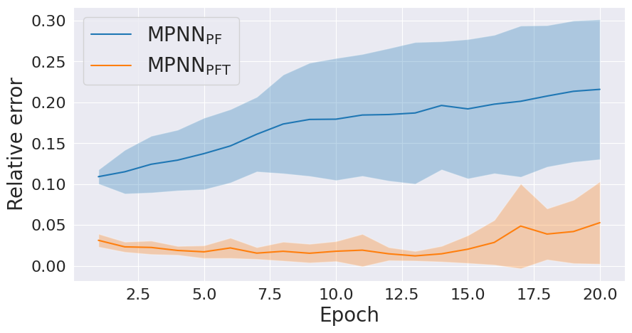
(a) Validation relative error per epoch

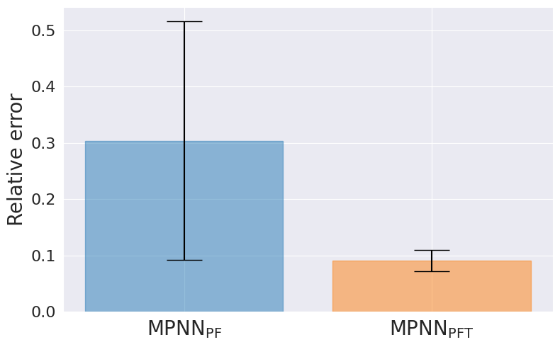
(b) Final test relative error

Figure 1: Standard transfer learning approaches are not applicable for our purposes: the resulting models are unable to generalise both in- and out-of-distribution.

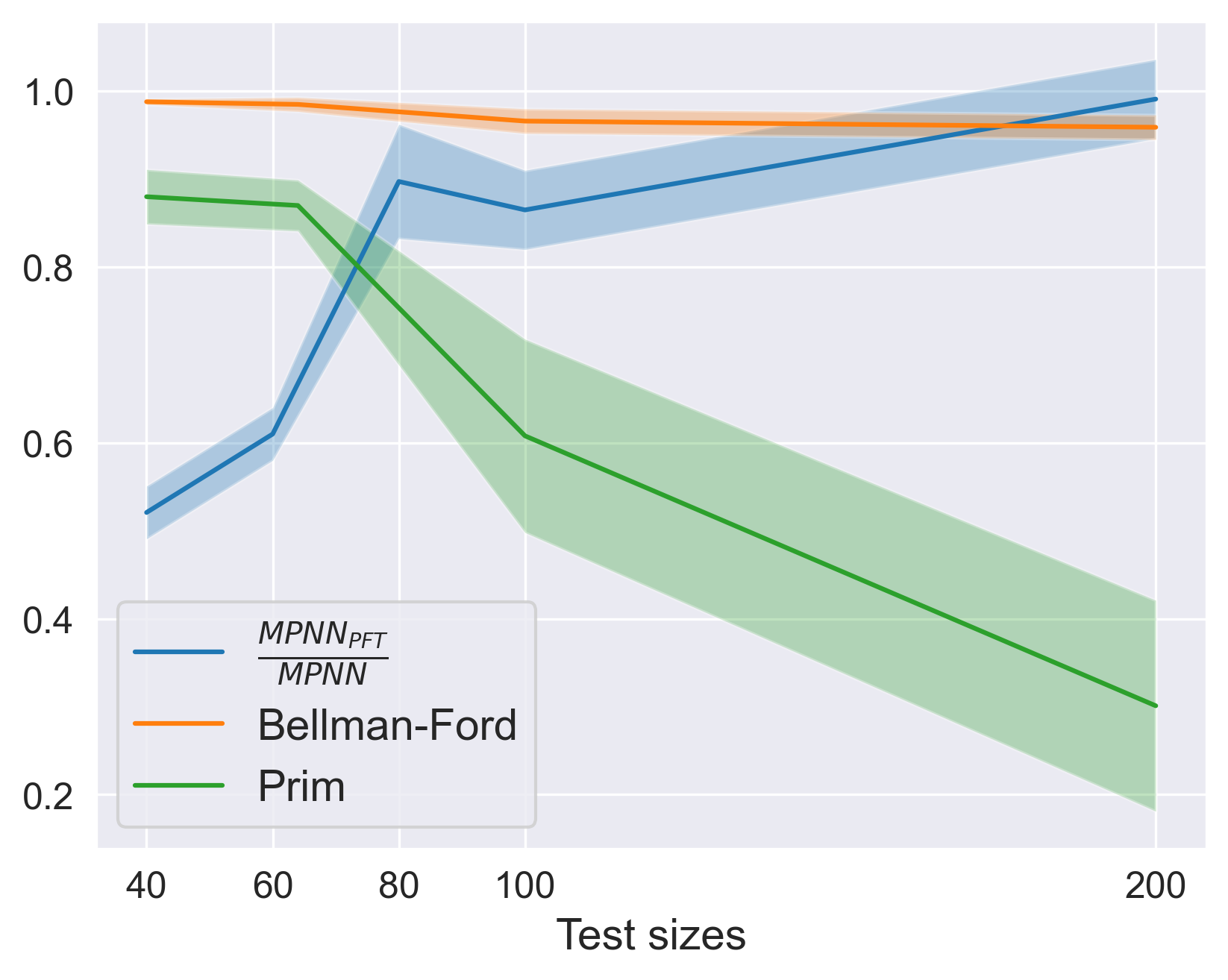
(a) MPNN_PFT initially outperforms MPNN most likely due to accurate MST predictions (Prim’s curve). However, as MPNN_PFT struggles with larger graphs, the performance gap narrows ($\frac{\text{MPNN\textsubscript{PFT}}}{\text{MPNN}}$ approaches 1).

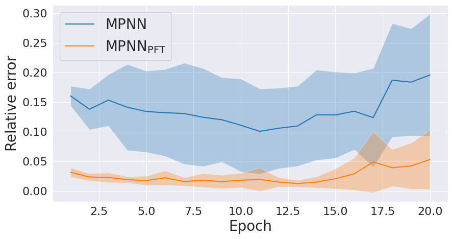
(b) Pre-training on algorithmic reasoning converges faster. Both models use the same architecture and hyperparameters.

Figure 2: Comparative analysis: (a) MPNN_PFT vs. MPNN performance, and (b) Convergence speed with algorithmic reasoning pre-training.

Standard transfer does not work

Classical approaches, e.g. as in XLVIN [11], do not produce good solutions. Contrasted to the fine-tuned model, which usually tends to achieve the best in-distribution validation loss around epoch 13-14, having one frozen processor tends to produce only worse performance with training, as evident in Figure 1. While for some target tasks $\mathcal{T}$ it may be desirable to be as faithful as possible to the base $\mathcal{B}$, our experiments suggest this is not the case here.

Table 1: TSP extrapolation relative error across different sizes. All models are trained on the same data of graphs up to size 20. MPNN denotes our base model without algorithmic knowledge. We added a subscript if we used edge hidden state or attempted knowledge transfer (cf. subsection 4.3). Note, that despite being a heuristic, LKH almost always produced optimal solutions.

	Test size
Model	40	60	80	100	200	1000
Beam search with width w=128
MPNN	$17.7_{\pm 5}\%$	$23.9_{\pm 3}\%$	$25.7_{\pm 8}\%$	$31.9_{\pm 6}\%$	$38.9_{\pm 7}\%$	$39.7_{\pm 7}\%$
GPS	$13.9_{\pm 1}\%$	$26.3_{\pm 2}\%$	$24.1_{\pm 4}\%$	$29.7_{\pm 5}\%$	$35.8_{\pm 4}\%$	$39.9_{\pm 2}\%$
MPNNPFT	$9.1_{\pm 0.1}\%$	$15.5_{\pm 4}\%$	$23.1_{\pm 3}\%$	$28.9_{\pm 2}\%$	$35.4_{\pm 2}\%$	$44.5_{\pm 9}\%$
MPNNPFT+ueh	$15.4_{\pm 5}\%$	$23.5_{\pm 8}\%$	$29.4_{\pm 7}\%$	$35.7_{\pm 6}\%$	$37.9_{\pm 3}\%$	$48.8_{\pm 14}\%$
MPNN2PROC	$12.2_{\pm 5}\%$	$22.1_{\pm 4}\%$	$28.4_{\pm 6}\%$	$34.0_{\pm 5}\%$	$36.6_{\pm 6}\%$	$38.8_{\pm 3}\%$
MPNNMTL	$18.1_{\pm 6}\%$	$26.2_{\pm 4}\%$	$31.2_{\pm 5}\%$	$34.8_{\pm 4}\%$	$37.1_{\pm 3}\%$	$38.5_{\pm 3}\%$
Joshi et al. (AR)	$6.2_{\pm 4}\%$	$37.1_{\pm 12}\%$	$74.8_{\pm 13}\%$	$102_{\pm 10}\%$	$195_{\pm 20}\%$	$419_{\pm 20}\%$
Joshi et al. (nAR)	$20.6_{\pm 10}\%$	$62.5_{\pm 11}\%$	$110_{\pm 17}\%$	$156_{\pm 24}\%$	$273_{\pm 24}\%$	$497_{\pm 7}\%$
Beam search with width w=1280
MPNN	$14.4_{\pm 4}\%$	$21.8_{\pm 5}\%$	$22.4_{\pm 4}\%$	$31.1_{\pm 6}\%$	$33.6_{\pm 3}\%$	$41.2_{\pm 8}\%$
GPS	$11.0_{\pm 1}\%$	$21.0_{\pm 1}\%$	$19.0_{\pm 3}\%$	$23.8_{\pm 5}\%$	$35.3_{\pm 6}\%$	$40.1_{\pm 2}\%$
MPNNPFT	$7.5_{\pm 1}\%$	$13.3_{\pm 3}\%$	$20.1_{\pm 5}\%$	$26.9_{\pm 3}\%$	$33.8_{\pm 2}\%$	$40.5_{\pm 7}\%$
MPNNPFT+ueh	$12.9_{\pm 5}\%$	$20.6_{\pm 6}\%$	$26.0_{\pm 3}\%$	$32.0_{\pm 5}\%$	$37.2_{\pm 3}\%$	$44.3_{\pm 9}\%$
MPNN2PROC	$9.5_{\pm 6}\%$	$18.0_{\pm 5}\%$	$24.1_{\pm 6}\%$	$28.8_{\pm 5}\%$	$36.6_{\pm 6}\%$	$38.5_{\pm 3}\%$
MPNNMTL	$15.5_{\pm 5}\%$	$26.5_{\pm 6}\%$	$30.2_{\pm 6}\%$	$33.4_{\pm 4}\%$	$36.8_{\pm 5}\%$	$42.3_{\pm 5}\%$
Joshi et al. (AR)	$3.5_{\pm 3}\%$	$33.0_{\pm 11}\%$	$63.8_{\pm 12}\%$	$97.6_{\pm 12}\%$	$193.3_{\pm 17}\%$	$417_{\pm 4}\%$
Joshi et al. (nAR)	$14.2_{\pm 8}\%$	$54.7_{\pm 15}\%$	$100.0_{\pm 15}\%$	$141.9_{\pm 25}\%$	$265.5_{\pm 27}\%$	$500.7_{\pm 23}\%$
Models not using beam search
Joshi et al. (AR+greedy)	$22.1_{\pm 10}\%$	$57.7_{\pm 13}\%$	$94.0_{\pm 14}\%$	$124.0_{\pm 12}\%$	$219.6_{\pm 22}\%$	$469_{\pm 17}\%$
Joshi et al. (AR+sampling)	$9.5_{\pm 5}\%$	$46.7_{\pm 9}\%$	$93.1_{\pm 10}\%$	$137.0_{\pm 14}\%$	$313.2_{\pm 15}\%$	$1102_{\pm 1}\%$
Deterministic baselines
Greedy	$31.9_{\pm 12}\%$	$32.8_{\pm 10}\%$	$33.3_{\pm 9}\%$	$30.0_{\pm 6}\%$	$32.1_{\pm 6}\%$	$28.8_{\pm 3}\%$
Beam search (w=1280)	$19.7_{\pm 8}\%$	$23.1_{\pm 7}\%$	$29.4_{\pm 7}\%$	$29.7_{\pm 5}\%$	$33.2_{\pm 4}\%$	$38.9_{\pm 2}\%$
Christofides	$10.1_{\pm 3}\%$	$11.0_{\pm 2}\%$	$11.3_{\pm 2}\%$	$12.1_{\pm 2}\%$	$12.2_{\pm 1}\%$	$12.2_{\pm 0.1}\%$
LKH	$0.0_{\pm 0.0}\%$	$0.0_{\pm 0.0}\%$	$0.0_{\pm 0.0}\%$	$0.0_{\pm 0.0}\%$	$0.0_{\pm 0.0}\%$	$0.01_{\pm 0.0}\%$

Transfer vs no-transfer

Our main results are presented in Table 1. We start by noting that except on the smallest test sizes, our model outperformed the architecture of Joshi et al., often by a significant margin. From our results, the latter architecture tends to fit well the training data distribution but exhibits worse OOD generalisation, as confirmed by results on $\geq$ 60 nodes.

Our next observation is that in almost all cases, pre-training our model to perform algorithms gives better performance even when compared to a more sophisticated baseline utilising the GPS graph transformer convolution [40]. Even though the performance gap diminishes as the test size increases, 2(a) suggests that this trend is influenced by the progressive deterioration of algorithmic reasoning performance as test graph size increases. In particular, one can note that MPNN and MPNN_PFT perform very similarly for graphs with $\geq$200 nodes. This observation aligns with the point where MPNN_PFT demonstrates its lowest performance on Prim’s algorithm, i.e. $\sim 30\%$. This suggests that building neural algorithmic reasoners that can strongly generalise even for much larger graphs becomes critical to solving CO problems using our approach.

Surprisingly, training two processors, i.e. MPNN_2PROC, did not yield performance gain when compared to MPNN_PFT, while outperforming the algorithm-agnostic baseline. In the original formulation from Xhonneux et al. the latent representations of the two processors are summed together. However, summing the two representations was unstable and led to crashes in our experiments. In our experiments, we used mean instead. MPNN_MTL also exhibited inferior performance compared to other models. In general, our results suggest that transforming knowledge from P to NP is not trivial. Specifically, we note that our pre-trained reasoners emit representations from which we can easily decode steps of Prim and Bellman-Ford. However, transforming this information into a “good heuristic” for the TSP can not be achieved by trivially linearly projecting it (MPNN_PF, see Figure 1), or by averaging it with a learnt representation for the TSP (MPNN_2PROC). Clearly, learning a representation that has to both encode information for P and NP (MPNN_MTL) did not lead to meaningful representations either, since it performs worse than a simple MPNN. We conclude that the best way of transforming such information to a good performing heuristic for an NP problem is to fine-tune the representations (MPNN_PFT).

Additionally, we noticed that when compared to a model with an identical architecture but without algorithmic knowledge, inducing algorithmic knowledge led to faster convergence and exhibited delayed overfitting compared to its corresponding non-pretrained model, as depicted in Figure 2(b).

Lastly, we note that we can outperform simpler non-parametric baselines on nearly all test sizes, i.e. greedy and beam search and we perform better and comparable to Christofides for 2x and 3x larger graphs. Unfortunately, all neural models still fall short at larger graphs and we are outperformed by LKH, which almost always produces optimal solutions. We hypothesise that with stronger algorithmic generalisation OOD we could match Christofides algorithm and that future studies could investigate integrating LKH with NAR (or vice versa).

Does it matter what we put in it?

An “alternative hypothesis” that one can make is that the improvements are due to the network being trained on the same data distribution and the algorithms themselves do not matter and any algorithm would suffice. We present two counterarguments: First, results in Appendix C show that selecting unrelated algorithms is subpar to selecting related ones and may also result in final bad local minima with poorer generalisation. However, when one is uncertain about what algorithms to pick, a generalist-like pre-training [27] may still be a viable option. Second, results in Appendix D show that changing the source data distribution does not lead to results worse than no transfer and may even produce better results at larger test sizes. Those two ablations suggest it is the algorithmic bias that is useful for learning CO problems.

5.4 VKC

Benchmarks

Given the strong performance of the PFT transfer learning variant and for computational efficiency, we concentrated on comparing best transfer versus no transfer, foregoing retesting of other transfer options with VKC. Additionally, we chose two deterministic baselines: the Gon algorithm, which influenced our algorithm selection, and the critical dominating set (CDS) heuristic [18]. Despite its poorer approximation ratio, CDS consistently provides good solutions in practice.

Table 2: VKC relative error. Each letter in the MPNNs’ subscript denotes an algorithm pre-trained on: Floyd-Warshall, Minumum, Insertion sort, Task scheduling, Bellman-Ford, Activity selection.

	Test size
Model	40	60	80	100	200
MPNN	$15.88_{\pm 1.11}\%$	$20.85_{\pm 2.64}\%$	$24.78_{\pm 7.17}\%$	$26.48_{\pm 6.65}\%$	$24.63_{\pm 6.50}\%$
MPNNFMITB	$14.73_{\pm 1.21}\%$	$21.97_{\pm 4.87}\%$	$23.91_{\pm 4.52}\%$	$28.50_{\pm 5.06}\%$	$27.04_{\pm 4.22}\%$
MPNNMTAB	$13.58_{\pm 0.60}\%$	$16.20_{\pm 3.02}\%$	$23.10_{\pm 3.99}\%$	$26.40_{\pm 6.62}\%$	$26.43_{\pm 3.84}\%$
Deterministic baselines
Farthest First	$41.04_{\pm 14.21}\%$	$43.89_{\pm 10.70}\%$	$38.31_{\pm 9.22}\%$	$36.32_{\pm 7.28}\%$	$37.91_{\pm 7.91}\%$
CDS	$7.15_{\pm 5.42}\%$	$7.82_{\pm 4.78}\%$	$6.49_{\pm 3.65}\%$	$6.55_{\pm 3.29}\%$	$5.98_{\pm 2.00}\%$

Results

Table 2 summarises our results with VKC. When picking algorithms, solely based on relevance to the task, we obtain results comparable, or worse than versions without pre-training. Removing the two poor performing algorithms (Floyd-Warshall, mean accuracy of $\approx 23\%$; Insertion Sort, $\approx 43\%$), in favour of an additional greedy (activity selection, $\approx 96\%$) results in a better model, substantially outperforming the baseline neural model at $2\times$ and $3\times$ extrapolation and tying for the other sizes. This further supports our hypothesis that generalising performance on algorithms is related to the performance on the downstream CO task.

Compared to the deterministic baselines, all neural models outperform the simpler heuristic. Unfortunately, even the best-performing models are not comparable to the CDS heuristic. We believe this is due to the fact that CDS consists of multiple, interlaced subroutines (binary search, graph pruning, etc.) and perhaps a future more modular NAR approach would give further performance boost.

6 Limitations and future work

Despite the promising results achieved in our study, there are still areas for improvement in current algorithmic reasoning networks, including our approach. In particular, the GNN requires $\mathcal{O}(N)$ message passing steps. This constraint makes training on very large graphs impractical (Appendix A). A future work direction we envision is NARs which require fewer iterations to execute an algorithm. Our intuition is based on Xu et al. [52] who, in their experiments of learning to find shortest paths, noted that a GNN may sometimes achieve satisfactory test accuracy with fewer iterations than the ground truth algorithm. Such a contribution, however, is out of the scope of this paper.

7 Conclusions

In this study, we explored the transfer of knowledge from algorithms in P to the travelling salesman problem and vertex k-center, both NP-hard combinatorial optimisation problems. Our findings revealed that standard transfer learning techniques did not yield satisfactory results. However, we observed that certain approaches, which were previously considered to have inferior performance, actually exhibited superior generalization capabilities and outperformed models that do not leverage pre-training on algorithms.

In conclusion, our findings provide strong evidence supporting the hypothesis that incorporating robust algorithmic knowledge is beneficial for achieving out-of-distribution generalization. By leveraging the insights from algorithms, we can enhance the performance of reasoning models on complex problems. These findings open up new avenues for the development of algorithmic reasoners that can effectively tackle challenging real-world tasks and applications.

Appendix A Runtime

Runtimes have been obtained on a A100 40GB GPU.

Table 3: Training and inference time on algorithms. This measures the efficiency of the pre-training phase. Time is relative to a single batch. Note that inference graphs are 4$\times$ the size of training graphs

	Training time (s)		Inference time (s)
	Erdős–Rényi	Cliques	Erdős–Rényi	Cliques
Bellman-Ford	$0.057$	$0.103$	$0.237$	$0.291$
Dijkstra	$0.160$	$0.184$	$1.469$	$3.004$
MST-Prim	$0.162$	$0.186$	$1.499$	$2.999$
MST-Kruskal	$1.576$	$2.073$	$32.997$	$44.957$
Floyd-Warshall	$0.231$	OOM (16GB)	$9.827$	OOM(16GB)

Table 4: Inference time of TSP solutions (in seconds). Time is relative to a single TSP of size $n$.

		Test size
	Model	20	40	60	80	100	200	1000
w=128	MPNN	$0.043$	$0.090$	$0.130$	$0.179$	$0.242$	$0.800$	$65.557$
w=1280	MPNN	$0.043$	$0.089$	$0.131$	$0.181$	$0.225$	$0.839$	$67.009$
	Greedy	$0.001$	$0.002$	$0.004$	$0.009$	$0.019$	$0.021$	$0.047$
	Christofides	$0.004$	$0.012$	$0.411$	$0.094$	$0.101$	$0.714$	$57.584$

Appendix B Algorithm selection rationale

Travelling Salesman Problem

TSP is defined on an undirected full graph, often originating from 2D Euclidean space. We thus considered graph and geometry algorithms in CLRS-30. Many of the algorithms were excluded as they were either trivial to solve on a full graph (e.g., BFS/articulation points), or were defined only on directed (acyclic) graphs (e.g., DFS, topological sort). We also excluded algorithms with long rollouts: e.g., in CLRS-30, MST-Kruskal and Dijkstra’s algorithms have (much) longer trajectories than MST-Prim and Bellman-Ford, despite having equal or better theoretical time complexity. Such long-trajectory algorithms are impractical for our application, as they result in higher training/inference times (Appendix A, Table 3). The resulting list, in the end, contained 3 relevant algorithms – Bellman-Ford, MST-Prim and Graham’s scan. Unfortunately in our initial experiments, integrating Graham led to poor performance and it was removed from our final models. We suspect this was due to the fact that NAR architectures do not incorporate invariance to Euclidean transformations [7].

Vertex k-center problem

The Vertex k-center problem employs a straightforward 2-approximation heuristic, commonly known as the Gon algorithm [20, 13]. This heuristic involves randomly selecting the first station and then greedily choosing the vertex that is farthest from any of the currently chosen vertices. To learn this heuristic, the model needs to perform shortest path calculations between nodes and understand concepts like maximum finding (or minimum of negatives) and/or sorting. Considering the greedy algorithm nature of the Gon algorithm, we decided to pre-train our model on Bellman-Ford, Minimum finding, and two CLRS-30 greedy problems: activity selection [19] and task scheduling [35]. The reason to choose Bellman-Ford over Floyd-Warshall (an all-pairs shortest path algorithm) and Minimum over Insertion sort is that Floyd-Warshall and Insertion sort have much poorer performance.

Appendix C On selecting unrelated algorithms

Table 5: TSP relative error comparison between no-transfer, transferring unrelated algorithms and transferring related algorithms. When transferring, the experimental setup matches MPNN_PFT, only algorithms differ

	Test size
Model	40	60	80	100	200
Beam search with width w=128
MPNN	$17.7_{\pm 5}\%$	$23.9_{\pm 3}\%$	$25.7_{\pm 8}\%$	$31.9_{\pm 6}\%$	$38.9_{\pm 7}\%$
Unrelated	$12.3_{\pm 2.2}\%$	$17.5_{\pm 3.1}\%$	$22.3_{\pm 3.1}\%$	$26.4_{\pm 2.6}\%$	$199.0_{\pm 373.3}\%$
Related	$9.1_{\pm 0.1}\%$	$15.5_{\pm 4}\%$	$23.1_{\pm 3}\%$	$28.9_{\pm 2}\%$	$35.4_{\pm 2}\%$

To evaluate the impact of selecting an appropriate algorithm for training, we conducted the following additional experiment. We utilized our best TSP algorithm transfer configuration while pre-training on three different algorithms: Breadth-First Search (which is trivial on fully-connected graphs), Topological Sorting (defined for directed acyclic graphs), and Longest Common Subsequence length (a string algorithm). Results are presented in Table 5. While transferring unrelated algorithms still brings improvements and is comparable at sizes 80 and 100, the model starts to “explode” at size 200 and it cannot provide as optimal solutions at sizes 40 and 60.

Appendix D Transfer from non-euclidean data distribution

To evaluate to what extent the data distribution matters when pre-training, we reran our PFT experiment, but this time pre-training the algorithms on graphs from the Erdős-Renyi distribution. Results are given in Table 6.

Table 6: Pre-training on Euclidean data versus pre-training on Erdős-Renyi graphs.

	Test size
Model	40	60	80	100	200	1000
Beam search with width w=128
MPNN	$17.7_{\pm 5}\%$	$23.9_{\pm 3}\%$	$25.7_{\pm 8}\%$	$31.9_{\pm 6}\%$	$38.9_{\pm 7}\%$	$39.7_{\pm 7}\%$
MPNNNON_EUC	$10.5_{\pm 3}\%$	$17.3_{\pm 4}\%$	$22.6_{\pm 3}\%$	$25.1_{\pm 3}\%$	$31.0_{\pm 2}\%$	$36.9_{\pm 2}\%$
MPNNEUC	$9.1_{\pm 0.1}\%$	$15.5_{\pm 4}\%$	$23.1_{\pm 3}\%$	$28.9_{\pm 2}\%$	$35.4_{\pm 2}\%$	$44.5_{\pm 9}\%$
Beam search with width w=1280
MPNN	$14.4_{\pm 4}\%$	$21.8_{\pm 5}\%$	$22.4_{\pm 4}\%$	$31.1_{\pm 6}\%$	$33.6_{\pm 3}\%$	$41.2_{\pm 8}\%$
MPNNNON_EUC	$8.5_{\pm 3}\%$	$16.0_{\pm 3}\%$	$20.0_{\pm 3}\%$	$23.0_{\pm 2}\%$	$30.3_{\pm 2}\%$	$37.5_{\pm 3}\%$
MPNNEUC	$7.5_{\pm 1}\%$	$13.3_{\pm 3}\%$	$20.1_{\pm 5}\%$	$26.9_{\pm 3}\%$	$33.8_{\pm 2}\%$	$40.5_{\pm 7}\%$

Appendix E Benchmarking versus CP/MIP

	Test size
Model	$40$	$60$	$80$	$100$	$200$	$1000$
Relative time limit
Gurobi ($1\times$)	$102.0_{\pm 133}\%$	$\bot$	$\bot$	$\bot$	$\bot$	$\bot$
Gurobi ($3\times$)	$15.0_{\pm 19}\%$	$35.0_{\pm 46}\%$	$\bot$	$\bot$	$\bot$	$\bot$
Gurobi ($5\times$)	$6.3_{\pm 9}\%$	$21.9_{\pm 15}\%$	$25.7_{\pm 18}\%$	$\bot$	$\bot$	$\bot$
Absolute time limit
Gurobi (3s)	$1.0_{\pm 2}\%$	$4.1_{\pm 4}\%$	$13.1_{\pm 11}\%$	$26_{\pm 27}\%$	$\bot$	$\bot$
Gurobi (5s)	$0.4_{\pm 1}\%$	$2.6_{\pm 3}\%$	$7.8_{\pm 7}\%$	$15_{\pm 15}\%$	$\bot$	$\bot$
Gurobi (10s)	$0.1_{\pm 0}\%$	$0.6_{\pm 1}$	$5.8_{\pm 5}\%$	$7_{\pm 6}\%$	$\bot$	$\bot$
Gurobi (30s)	$-$	$-$	$-$	$-$	$18_{\pm 12}\%$	$\bot$
Gurobi (60s)	$-$	$-$	$-$	$-$	$12_{\pm 9}\%$	$\bot$
Gurobi ($\infty$s)	$-$	$-$	$-$	$-$	$-$	$OOM(30GB)$

Table 7: Relative error of the solution Gurobi provided, given the time limit. Relative time limit is respectively $1\times,3\times$ and $5\times$ the runtime of our model, as taken from Table 4. $\bot$ means the solver did not produce a solution within the time constraint. We decided not to run experiments with $-$ – while we have not seen it, based on previous experiments and relative improvements we assume Gurobi would have found the optimal solutions.

We will start this appendix by noting that CP and MIP solvers would always produce the optimal solution if provided with sufficient compute time. We therefore will be comparing with such solvers after setting a time limit for their computation. As such solvers leverage CPU multithreading, all experiments will be performed on a 16-thread AMD Ryzen 5000 series CPU. Note, that in vanilla TSP those approaches may also be costly to compute, and CP works better for problems having a lot of combinatorial constraints, such as TSP with time windows [43].

Our initial experiment with more sophisticated baselines and constraint programming concretely was using Gecode interfaced through Zython. Unfortunately solving a single TSP instance of size 40 took nearly 2600 seconds and the dataset consists of 1000 such samples. We therefore did not continue further experiments and switched to Gurobi, which could solve examples of this size in just a couple of seconds.

We performed two kinds of experiments with Gurobi. One with a relative time limit ($1\times,3\times,5\times$ of our model inference time) and one with an absolute time limit (always larger than corresponding $5\times$). Across all variants, the TSP problem was formulated using the Miller-Tucker-Zemlin integer programming formulation [37] and we used the default Gurobi configuration (by not setting any environmental variables of PuLP). Results are presented in Table 7. At $1\times$ and $3\times$ Gurobi produced worse solutions than our best model and only produced better solutions for the smallest size at $5\times$. Solution quality did improve as time was increased, but at the larger sizes, Gurobi needed more than 30s to produce a solution and ran out of memory (OOM) at the largest size, without producing a solution.

Unfortunately, we still fall short of Concorde, which always found the optimal solution even at the strictest time constraints, even though it does not always prove the optimality. Note, however, that Concorde is highly specialised in solving TSP instances. It is our belief that models aligned to parallel algorithms [14] would help improve runtimes, leading to GNNs eventually outperforming Concorde.

References

- Applegate et al. [2006] D. Applegate, R. Bixby, V. Chvatal, and W. Cook. Concorde tsp solver, 2006.
- Bacciu et al. [2020] D. Bacciu, F. Errica, A. Micheli, and M. Podda. A gentle introduction to deep learning for graphs. Neural Networks, 129:203–221, 2020.
- Balas and Toth [1983] E. Balas and P. Toth. Branch and bound methods for the traveling salesman problem. 1983.
- Baniasadi et al. [2020] P. Baniasadi, M. Foumani, K. Smith-Miles, and V. Ejov. A transformation technique for the clustered generalized traveling salesman problem with applications to logistics. European Journal of Operational Research, 285(2):444–457, 2020.
- Bello et al. [2017] I. Bello, H. Pham, Q. V. Le, M. Norouzi, and S. Bengio. Neural combinatorial optimization with reinforcement learning. In 5th International Conference on Learning Representations, ICLR 2017, Toulon, France, April 24-26, 2017, Workshop Track Proceedings. OpenReview.net, 2017. URL https://openreview.net/forum?id=Bk9mxlSFx.
- Bhattacharya et al. [2017] S. Bhattacharya, M. Henzinger, and D. Nanongkai. Fully dynamic approximate maximum matching and minimum vertex cover in o (log3 n) worst case update time. In Proceedings of the Twenty-Eighth Annual ACM-SIAM Symposium on Discrete Algorithms, pages 470–489. SIAM, 2017.
- Bronstein et al. [2021] M. M. Bronstein, J. Bruna, T. Cohen, and P. Veličković. Geometric deep learning: Grids, groups, graphs, geodesics, and gauges. arXiv preprint arXiv:2104.13478, 2021.
- Christofides [1976] N. Christofides. Worst-case analysis of a new heuristic for the travelling salesman problem. Technical report, Carnegie-Mellon Univ Pittsburgh Pa Management Sciences Research Group, 1976.
- Cormen et al. [2009] T. H. Cormen, C. E. Leiserson, R. L. Rivest, and C. Stein. Introduction to Algorithms, 3rd Edition. MIT Press, 2009. ISBN 978-0-262-03384-8. URL http://mitpress.mit.edu/books/introduction-algorithms.
- Deac et al. [2020] A. Deac, P. Veličković, O. Milinković, P.-L. Bacon, J. Tang, and M. Nikolić. Xlvin: executed latent value iteration nets. In Learning Meets Combinatorial Algorithms at NeurIPS2020, 2020.
- Deac et al. [2021] A. Deac, P. Velickovic, O. Milinkovic, P. Bacon, J. Tang, and M. Nikolic. Neural algorithmic reasoners are implicit planners. In NeurIPS, pages 15529–15542, 2021.
- Deudon et al. [2018] M. Deudon, P. Cournut, A. Lacoste, Y. Adulyasak, and L.-M. Rousseau. Learning heuristics for the tsp by policy gradient. In W.-J. van Hoeve, editor, Integration of Constraint Programming, Artificial Intelligence, and Operations Research, pages 170–181, Cham, 2018. Springer International Publishing. ISBN 978-3-319-93031-2.
- Dyer and Frieze [1985] M. Dyer and A. Frieze. A simple heuristic for the p-centre problem. Operations Research Letters, 3(6):285–288, 1985. ISSN 0167-6377. doi: https://doi.org/10.1016/0167-6377(85)90002-1. URL https://www.sciencedirect.com/science/article/pii/0167637785900021.
- Engelmayer et al. [2023] V. Engelmayer, D. Georgiev, and P. Veličković. Parallel algorithms align with neural execution. arXiv preprint arXiv:2307.04049, 2023.
- Erdős et al. [1960] P. Erdős, A. Rényi, et al. On the evolution of random graphs. Publ. Math. Inst. Hung. Acad. Sci, 5(1):17–60, 1960.
- Fey and Lenssen [2019] M. Fey and J. E. Lenssen. Fast graph representation learning with PyTorch Geometric. In ICLR Workshop on Representation Learning on Graphs and Manifolds, 2019.
- Ford Jr [1956] L. R. Ford Jr. Network flow theory. Technical report, Rand Corp Santa Monica Ca, 1956.
- Garcia-Diaz et al. [2017] J. Garcia-Diaz, J. J. Sanchez-Hernandez, R. Menchaca-Mendez, and R. Menchaca-Méndez. When a worse approximation factor gives better performance: a 3-approximation algorithm for the vertex k-center problem. J. Heuristics, 23(5):349–366, 2017. doi: 10.1007/s10732-017-9345-x. URL https://doi.org/10.1007/s10732-017-9345-x.
- Gavril [1972] F. Gavril. Algorithms for minimum coloring, maximum clique, minimum covering by cliques, and maximum independent set of a chordal graph. SIAM Journal on Computing, 1(2):180–187, 1972. doi: 10.1137/0201013. URL https://doi.org/10.1137/0201013.
- Gonzalez [1985] T. F. Gonzalez. Clustering to minimize the maximum intercluster distance. Theoretical Computer Science, 38:293–306, 1985. ISSN 0304-3975. doi: https://doi.org/10.1016/0304-3975(85)90224-5. URL https://www.sciencedirect.com/science/article/pii/0304397585902245.
- Gurobi Optimization, LLC [2023] Gurobi Optimization, LLC. Gurobi Optimizer Reference Manual, 2023. URL https://www.gurobi.com.
- Hakimi [1964] S. L. Hakimi. Optimum locations of switching centers and the absolute centers and medians of a graph. Operations research, 12(3):450–459, 1964.
- Hamrick et al. [2018] J. B. Hamrick, K. R. Allen, V. Bapst, T. Zhu, K. R. McKee, J. B. Tenenbaum, and P. W. Battaglia. Relational inductive bias for physical construction in humans and machines. arXiv preprint arXiv:1806.01203, 2018.
- Helsgaun [2000] K. Helsgaun. An effective implementation of the lin–kernighan traveling salesman heuristic. European journal of operational research, 126(1):106–130, 2000.
- Hochbaum and Shmoys [1985] D. S. Hochbaum and D. B. Shmoys. A best possible heuristic for the k-center problem. Mathematics of operations research, 10(2):180–184, 1985.
- Hopfield and Tank [1985] J. J. Hopfield and D. W. Tank. “neural” computation of decisions in optimization problems. Biological cybernetics, 52(3):141–152, 1985.
- Ibarz et al. [2022] B. Ibarz, V. Kurin, G. Papamakarios, K. Nikiforou, M. Bennani, R. Csordás, A. J. Dudzik, M. Bosnjak, A. Vitvitskyi, Y. Rubanova, A. Deac, B. Bevilacqua, Y. Ganin, C. Blundell, and P. Velickovic. A generalist neural algorithmic learner. In B. Rieck and R. Pascanu, editors, Learning on Graphs Conference, LoG 2022, 9-12 December 2022, Virtual Event, volume 198 of Proceedings of Machine Learning Research, page 2. PMLR, 2022. URL https://proceedings.mlr.press/v198/ibarz22a.html.
- Johnson and Liu [2006] O. Johnson and J. Liu. A traveling salesman approach for predicting protein functions. Source Code for Biology and Medicine, 1(1):3, 2006. doi: 10.1186/1751-0473-1-3. URL https://doi.org/10.1186/1751-0473-1-3.
- Joshi et al. [2022] C. K. Joshi, Q. Cappart, L.-M. Rousseau, and T. Laurent. Learning the travelling salesperson problem requires rethinking generalization. Constraints, 27(1-2):70–98, 2022.
- Karlin et al. [2022] A. R. Karlin, N. Klein, and S. O. Gharan. A (slightly) improved approximation algorithm for metric tsp, 2022.
- Khalil et al. [2017] E. B. Khalil, H. Dai, Y. Zhang, B. Dilkina, and L. Song. Learning combinatorial optimization algorithms over graphs. In I. Guyon, U. von Luxburg, S. Bengio, H. M. Wallach, R. Fergus, S. V. N. Vishwanathan, and R. Garnett, editors, Advances in Neural Information Processing Systems 30: Annual Conference on Neural Information Processing Systems 2017, December 4-9, 2017, Long Beach, CA, USA, pages 6348–6358, 2017. URL https://proceedings.neurips.cc/paper/2017/hash/d9896106ca98d3d05b8cbdf4fd8b13a1-Abstract.html.
- Kingma and Ba [2015] D. P. Kingma and J. Ba. Adam: A method for stochastic optimization. In Y. Bengio and Y. LeCun, editors, 3rd International Conference on Learning Representations, ICLR 2015, San Diego, CA, USA, May 7-9, 2015, Conference Track Proceedings, 2015. URL http://arxiv.org/abs/1412.6980.
- Kipf and Welling [2017] T. N. Kipf and M. Welling. Semi-supervised classification with graph convolutional networks. In International Conference on Learning Representations, 2017. URL https://openreview.net/forum?id=SJU4ayYgl.
- Kool et al. [2019] W. Kool, H. van Hoof, and M. Welling. Attention, learn to solve routing problems!, 2019.
- Lawler [2001] E. L. Lawler. Combinatorial optimization: networks and matroids. Courier Corporation, 2001.
- Mahdavi et al. [2023] S. Mahdavi, K. Swersky, T. Kipf, M. Hashemi, C. Thrampoulidis, and R. Liao. Towards better out-of-distribution generalization of neural algorithmic reasoning tasks. Transactions on Machine Learning Research, 2023. ISSN 2835-8856. URL https://openreview.net/forum?id=xkrtvHlp3P.
- Miller et al. [1960] C. E. Miller, A. W. Tucker, and R. A. Zemlin. Integer programming formulation of traveling salesman problems. Journal of the ACM (JACM), 7(4):326–329, 1960.
- Numeroso et al. [2023] D. Numeroso, D. Bacciu, and P. Veličković. Dual algorithmic reasoning. In ICLR. OpenReview.net, 2023.
- Prim [1957] R. C. Prim. Shortest connection networks and some generalizations. The Bell System Technical Journal, 36(6):1389–1401, 1957.
- Rampášek et al. [2022] L. Rampášek, M. Galkin, V. P. Dwivedi, A. T. Luu, G. Wolf, and D. Beaini. Recipe for a general, powerful, scalable graph transformer. Advances in Neural Information Processing Systems, 35:14501–14515, 2022.
- Richard [1958] B. Richard. On a routing problem. Quarterly of Applied Mathematics, 16(1):87–90, 1958.
- Sankoff and Blanchette [1998] D. Sankoff and M. Blanchette. Multiple genome rearrangement and breakpoint phylogeny. Journal of computational biology, 5(3):555–570, 1998.
- Savelsbergh [1985] M. W. Savelsbergh. Local search in routing problems with time windows. Annals of Operations research, 4:285–305, 1985.
- [44] H. Strathmann, M. Barekatain, C. Blundell, and P. Veličković. Persistent message passing. In ICLR 2021 Workshop on Geometrical and Topological Representation Learning.
- Velickovic and Blundell [2021] P. Velickovic and C. Blundell. Neural algorithmic reasoning. Patterns, 2(7):100273, 2021. doi: 10.1016/j.patter.2021.100273. URL https://doi.org/10.1016/j.patter.2021.100273.
- Veličković et al. [2020] P. Veličković, L. Buesing, M. Overlan, R. Pascanu, O. Vinyals, and C. Blundell. Pointer graph networks. Advances in Neural Information Processing Systems, 33:2232–2244, 2020.
- Velickovic et al. [2020] P. Velickovic, R. Ying, M. Padovano, R. Hadsell, and C. Blundell. Neural execution of graph algorithms. In ICLR. OpenReview.net, 2020.
- Veličković et al. [2022] P. Veličković, A. P. Badia, D. Budden, R. Pascanu, A. Banino, M. Dashevskiy, R. Hadsell, and C. Blundell. The clrs algorithmic reasoning benchmark. In International Conference on Machine Learning, pages 22084–22102. PMLR, 2022.
- Veličković et al. [2018] P. Veličković, G. Cucurull, A. Casanova, A. Romero, P. Liò, and Y. Bengio. Graph attention networks. In International Conference on Learning Representations, 2018. URL https://openreview.net/forum?id=rJXMpikCZ.
- Vinyals et al. [2015] O. Vinyals, M. Fortunato, and N. Jaitly. Pointer networks. In Proceedings of the 28th International Conference on Neural Information Processing Systems-Volume 2, pages 2692–2700, 2015.
- Xhonneux et al. [2021] S. Xhonneux, A. Deac, P. Velickovic, and J. Tang. How to transfer algorithmic reasoning knowledge to learn new algorithms? In NeurIPS, pages 19500–19512, 2021.
- Xu et al. [2020] K. Xu, J. Li, M. Zhang, S. S. Du, K. ichi Kawarabayashi, and S. Jegelka. What can neural networks reason about? In International Conference on Learning Representations, 2020. URL https://openreview.net/forum?id=rJxbJeHFPS.
- Xu and Che [2019] Y. Xu and C. Che. A brief review of the intelligent algorithm for traveling salesman problem in uav route planning. In 2019 IEEE 9th international conference on electronics information and emergency communication (ICEIEC), pages 1–7. IEEE, 2019.