Cross correlations of the CMB Doppler mode and the 21 cm brightness temperature in the presence of a primordial magnetic field

Abstract

The cross correlation between the CMB Doppler mode and the 21 cm line brightness temperature is calculated in the presence of a stochastic primordial magnetic field. Potential detectability is estimated for Planck 2018 bestfit parameters in combination with configuration and survey design parameters of 21 cm line radio telescopes such as LOFAR and the future SKAO. Homogeneous as well as inhomogeneous reionization has been considered. In particular the latter in combination with SKA1-mid shows promising signal-over-noise ratios.

I Introduction

There is ample evidence for magnetic fields being present in galaxies and clusters of galaxies and even in filaments on scales beyond clusters. All of these observations associate magnetic fields with collapsed structures. Since about the last decade observational data of a number of blazars have been interpreted as evidence of the presence of magnetic fields in voids. This could indicate the existence of cosmological magnetic fields not associated with any virialized structure but rather pervading the observable universe as a whole. These latter observations together with for example the question of the origin of galactic magnetic fields motivate the consideration of a primordial magnetic field (for reviews, e.g., Durrer and Neronov (2013); Kandus et al. (2011)).

If these large scale magnetic fields are generated in the very early universe before decoupling cosmological observables such as, e.g., the temperature anisotropies and polarization of the cosmic microwave background (CMB) are affected. There are several ways how cosmological magnetic fields enter into the dynamics of cosmological perturbations that eventually leave their imprint on the angular power spectra of the CMB (cf. e.g., Giovannini (2004); Giovannini and Kunze (2008); Paoletti et al. (2009); Kahniashvili and Ratra (2005); Shaw and Lewis (2010); Kunze (2011); Shaw and Lewis (2012); Kunze (2012)). Directly magnetic fields contribute to the total energy and anisotropic stress perturbations as well as to the evolution of the baryon velocity perturbations. Indirectly they have an important effect because of their dissipation due to the interaction with the cosmic plasma. This leads to additional energy injection and heating of matter Sethi and Subramanian (2005); Kunze and Komatsu (2015).

Motivated by the observed isotropy of the universe on very large scales primordial magnetic fields are assumed to be gaussian random fields. Various observations, such as the CMB, limit their present day amplitude to be of order of nG or below (cf. e.g. Ade et al. (2016)). Current and upcoming observations of the 21 cm line of neutral hydrogen provide new opportunities of constraining the parameters of a putative primordial magnetic field.

Over the last three decades observations of the CMB have opened a window to the physics of the very early universe. The angular power spectrum of the temperature anisotropies, the E-mode of polarization and their cross correlation have been measured with unprecedented precision. The search for a putative primordial B-mode of the linear polarization is still going on. Since the first observations of quasars and the Gunn-Petersen trough it is known that the universe at least since a redshift of $z=6$ is reionized. Observations of the CMB temperature anisotropies and polarization such as the Planck 2018 data indicate a best fit value for the $\Lambda$CDM base model of $z=7.68$ Aghanim et al. (2020). This assumes nearly instanteneous reionization. Observations of the 21 cm line signal resulting from the hyperfine transition of neutral hydrogen measured against the CMB radiation is very sensitive to the epoch of reionization. Thus current and upcoming experiments dedicated to the observation of the cosmic 21 cm line signal will provide an insight into the details of the reionization epoch. Moreover, since the neutral hydrogen distribution traces the total matter distribution in the universe also details of the latter will be open to observations. In addition taking into account the redshifting of the 21 cm line signal observations at different frequencies correspond to different redshifts and thus different stages in the evolution of the universe (for reviews, e.g., Furlanetto et al. (2006); Loeb and Furlanetto (2013)). Since primordial magnetic fields have a direct effect on the linear matter power spectrum on small scales the cosmic 21 cm line signal provides an interesting probe into their existence. In Kunze (2019) the resulting 21 cm line signal has been obtained from simulations with the Simfast21 code Santos et al. (2010); Hassan et al. (2016) using this modified linear matter power spectrum as initial condition.

One of the effects of reionization is the rescattering of photons leading to a secondary Doppler contribution in the CMB anisotropies which is determined by the matter power spectrum. The cross correlation with the 21 cm signal has been first studied in Alvarez et al. (2006) with the objective to constrain the parameters of the reionization model and subsequently in Adshead and Furlanetto (2008).

The aim here is to study this cross correlation in the presence of a primordial magnetic field and the prospects to constrain the magnetic field parameters using the characteristics of radio telescope arrays such as the upcoming Square Kilometre Array Observatory (SKAO) with the updated specifications Dewdney (2015) as well as the already operational Low Frequency Array (LOFAR) van Haarlem et al. (2013). In the numerical solutions the best fit parameters of the base model derived from Planck 2018 data only are used Aghanim et al. (2020), in particular, $\Omega_{b}h^{2}$ = 0.022383, $\Omega_{m}h^{2}$ =0.14314, $H_{0}=67.32$ km s^-1Mpc^-1 and for the adiabatic mode $A_{s}=2.101\times 10^{-9}$ and $n_{s}=0.96605$. The angular power spectra of the CMB temperature anisotropies, the linear matter power spectra as well as other required functions of the cosmological background in the numerical solutions are calculated for the adiabatic mode and the compensated magnetic mode with a modified version of the CLASS code Kunze (2021) (for references of the original CLASS code cf Lesgourgues (2011a); Blas et al. (2011); Lesgourgues (2011b); Lesgourgues and Tram (2011, 2014)).

II The signals

Observations of the CMB indicate that the largest contribution to the total density perturbation is due to the adiabatic, primordial curvature mode (e.g.,Aghanim et al. (2020)). For the magnetic field contribution initial conditions corresponding to the compensated magnetic mode are chosen for the CMB Doppler mode as well as the linear matter power spectrum. For this type of initial condition the neutrino anisotropic stress approaches after neutrino decoupling a solution compensating the contribution of the anisotropic stress of the magnetic field Shaw and Lewis (2010); Kunze (2011, 2012). Having a behaviour similar to an isocurvature mode its contribution has to be subleading in comparison to the adiabatic mode.

The magnetic field ${\bf B}$ is assumed to be a non helical, gaussian random field determined by its two point function in $k$-space,

$$\langle B_{i}^{*}(\vec{k})B_{j}(\vec{q})\rangle=(2\pi)^{3}\delta({\vec{k}-\vec{q}})P_{B}(k)\left(\delta_{ij}-\frac{k_{i}k_{j}}{k^{2}}\right),$$ (2.1)

where the power spectrum, $P_{B}(k)$ is given by Kunze (2011)

$$P_{B}(k,k_{m},k_{L})=A_{B}\left(\frac{k}{k_{L}}\right)^{n_{B}}{\cal W}(k,k_{m})$$ (2.2)

with $A_{B}$ its amplitude, $k_{L}$ a pivot wave number chosen to be 1 Mpc^-1 and ${\cal W}(k,k_{m})=\pi^{-3/2}k_{m}^{-3}e^{-(k/k_{m})^{2}}$ a gaussian window function. $k_{m}$ corresponds to the largest scale damped due to radiative viscosity before decoupling Subramanian and Barrow (1998); Jedamzik et al. (1998). $k_{m}$ has its largest value at recombination

$$k_{m}=301.45\left(\frac{B}{\rm nG}\right)^{-1}{\rm Mpc}^{-1}$$ (2.3)

for the bestfit parameters of Planck 2018 data only Kunze (2021); Aghanim et al. (2020).

II.1 The 21 cm line signal: Auto correlation

The cosmic 21 cm line signal corresponds to the change in the brightness temperature of the CMB which in general depends on direction ${\bf n}$ and redshift $z$. An overline indicates the corresponding homogeneous background variable. Expanding the differential brightness temperature of the 21 cm signal upto first order, $T_{21}({\bf n},z)=\overline{T}_{21}(z)+\delta T_{21}({\bf n},z)$, the observed differential brightness perturbation corresponding to the cosmic 21 cm line signal originating at a redshift $z$ is given by Zaldarriaga et al. (2004); Alvarez et al. (2006); Adshead and Furlanetto (2008)

$$T_{21}({\bf n},z)=T_{0}(z)\int_{0}^{\eta_{0}}d\eta^{\prime}W\left[\eta(z)-\eta^{\prime}\right]\psi_{21}({\bf n},\eta^{\prime}),$$ (2.4)

where $\eta$ is conformal time and $W(x)$ denotes the spectral response function of the instrument which for simplicity is chosen to be a $\delta$ function, $W(x)=\delta(x)$. The signal generated by regions of neutral hydrogen at redshift $z$ will be observed today at $\nu_{21cm}=1420.4057\;{\rm MHz}/(1+z)$. Moreover Adshead and Furlanetto (2008) ,

$$T_{0}(z) = 23{\rm mK}\left(\frac{\Omega_{b}h^{2}}{0.02}\right)\left[\left(\frac{0.15}{\Omega_{m}h^{2}}\right)\left(\frac{1+z}{10}\right)\right]^{\frac{1}{2}},$$ (2.5)

$$\psi_{21}({\bf n},\eta), = x_{H}({\bf n},\eta)\left(1+\delta_{b}({\bf n},\eta)-\frac{1}{a(\eta)H(\eta)}\frac{\partial v_{r}}{\partial r}\right)\left(1-\frac{T_{CMB}}{T_{s}({\bf n},\eta)}\right),$$ (2.6)

where $\delta_{b}$ is the baryon energy density contrast, $x_{H}$ refers to the fraction of neutral hydrogen and as in Adshead and Furlanetto (2008) the effect of redshift space distortion upto linear order is included. This is due to the fact that the peculiar velocity of distant, massive objects leads to a distortion of their position in redshift space Kaiser (1987); Shaw and Lewis (2008).

From around the beginning of reionization it can be assumed that the spin temperature $T_{s}$ of neutral hydrogen is much higher than the one of the CMB. Using equation (2.6) together with $\psi({\bf n},z)=\overline{\psi}_{21}(z)+\delta\psi_{21}({\bf n},z)$ implies $\overline{T}_{21}(z)=T_{0}(z)x_{H}(z)$ and $\delta T_{21}({\bf n},z)=T_{0}(z)\delta\psi_{21}({\bf n},\eta)$. Taking into account the possibility of inhomogeneous reionization then

$$\delta\psi_{21}({\bf n},\eta)=D(\eta)\left[\bar{x}_{H}(\eta)\delta_{b}({\bf n,\eta_{0}})-\bar{x}_{e}\delta_{x}({\bf n,\eta_{0}})\right]-\frac{\overline{x}_{H}(\eta)}{a(\eta)H(\eta)}\frac{\partial v_{r}}{\partial r}$$ (2.7)

where $D(\eta)$ is the growth factor of the baryon density perturbation $\delta_{b}$ during matter domination. Moreover, it is assumed that the time evolution of the ionization fraction perturbation $\delta_{x}=(x_{e}-\bar{x}_{e})/\bar{x}_{e}$ follows that of the linear matter perturbation. The total baryon density perturbation is given by $\delta_{b,tot}=\delta_{b,ad}+\delta_{b,B}$ including both the adiabatic primordial curvature mode and the magnetic mode. During matter domination the evolution of the energy density perturbation of the magnetic mode follows that of the adiabatic mode so that $\delta_{b,tot}({\bf k},\eta)=D(\eta)\delta_{b,tot}({\bf k},\eta_{0})$ which follows the evolution of the total matter density perturbation $\delta_{m,tot}$ (e.g. Kunze (2014)). Finally, the baryon velocity perturbation is determined by $v=-\dot{\delta}_{b}/k$ Kodama and Sasaki (1984).

Following Zaldarriaga et al. (2004); Alvarez et al. (2006); Adshead and Furlanetto (2008) expanding $\delta\psi_{21}({\bf n},\eta)$ in terms of spherical harmonics (e.g. Hu and White (1997)) yields the corresponding expansion coefficients for the 21 cm line signal brightness perturbation as,

$$a^{(21)}_{\ell m} = 4\pi(-i)^{\ell}T_{0}(z)\sum_{\bf k}\left[D(\eta)\left[\bar{x}_{H}(\eta)\delta_{b}({\bf k})-\bar{x}_{e}(\eta)\delta_{x}({\bf k})\right]j_{\ell}(k(\eta_{0}-\eta(z)))\right.$$ (2.8)

$$+\left.\frac{\bar{x}_{H}(\eta)k}{a(\eta)H(\eta)}j_{\ell}^{\prime\prime}(k(\eta_{0}-\eta(z)))v({\bf k},\eta)\right]Y_{\ell m}^{*}({\bf\hat{k}}),$$

where

$$j_{\ell}^{\prime\prime}(w)=\frac{\ell(\ell-1)}{(2\ell+1)(2\ell-1)}j_{\ell-2}(w)-\frac{2\ell^{2}+2\ell-1}{(2\ell-1)(2\ell+3)}j_{\ell}(w)+\frac{(\ell+1)(\ell+2)}{(2\ell+1)(2\ell+3)}j_{\ell+2}(w).$$ (2.9)

In general the correlation functions of two modes $X$ and $Y$, respectively, are defined in terms of angular power spectra $C_{\ell}^{(XY)}$ such that

$$\langle a^{(X)}_{\ell^{\prime}m^{\prime}}a^{(Y)*}_{\ell m}\rangle=C^{(XY)}_{\ell}\delta_{\ell\ell^{\prime}}\delta_{mm^{\prime}}.$$ (2.10)

The autocorrelation function of the 21 cm line signal from redshift $z$ is determined by the angular power spectrum

$$C_{\ell}^{(21-21)}(z) = \frac{2}{\pi}T_{0}(z)^{2}D(\eta)^{2}$$ (2.11)

$$\times \int dkk^{2}\left[\left[\bar{x}_{H}(z)^{2}P_{m,tot}(k)-2\bar{x}_{H}(z)\bar{x}_{e}(z)P_{\delta_{m}\delta x}(k)+\bar{x}_{e}(z)^{2}P_{\delta x\delta x}(k)\right]j_{\ell}(w)j_{\ell}(w)\right.$$

$$- \left.2\bar{x}_{H}(z)\left[\bar{x}_{H}(z)P_{m,tot}(k)-\bar{x}_{e}(z)P_{\delta_{m}\delta x}(k)\right]j_{\ell}(w)j_{\ell}^{\prime\prime}(w)\right.$$

$$+ \left.\bar{x}_{H}(z)^{2}P_{m,tot}(k)j_{\ell}^{\prime\prime}(w)j_{\ell}^{\prime\prime}(w)\right],$$

where $w=k(\eta_{0}-\eta(z))$. Moreover, $P_{\delta_{m}\delta x}(k)$ denotes the cross correlation power spectrum of the ionized fraction and matter density perturbations. The autocorrelation power spectrum of the matter density perturbation is given by $P_{m}(k)$ and of the ionization fraction perturbation by $P_{\delta x\delta x}(k)$.

In the approximation for large $\ell$ it is found that

$$C_{\ell}^{(21-21)}(z) =\frac{2T_{0}(z)^{2}D(\eta)^{2}}{[\eta_{0}-\eta(z)]^{3}}\left[\frac{x_{\ell,max}^{(1)}}{4}\left[\bar{x}_{H}(z)^{2}P_{m,tot}(k_{\ell}^{(1)})-2\bar{x}_{H}(z)\bar{x}_{e}(z)P_{\delta_{m}\delta x}(k_{\ell}^{(1)})\right.\right.$$ (2.12)

$$\left.\left.\hskip 119.50148pt+\bar{x}_{e}(z)^{2}P_{\delta x\delta x}(k_{\ell}^{(1)})\right]\right.$$

$$- \left.\frac{[x_{\ell,max}^{(2)}]^{2}(1-2\ell(\ell+1))}{(3+2\ell)(4\ell^{2}-1)}\bar{x}_{H}(z)\left[\bar{x}_{H}(z)P_{m,tot}(k_{\ell}^{(2)})-\bar{x}_{e}(z)P_{\delta_{m}\delta x}(k_{\ell}^{(2)})\right]\right.$$

$$+ \left.\frac{3[x_{\ell,max}^{(3)}]^{2}[3+2\ell(\ell+1)(\ell^{2}+\ell-4)]}{2(4\ell^{2}-9)(4\ell-1)(5+2\ell)}\bar{x}_{H}(z)^{2}P_{m,tot}(k_{\ell}^{(3)})\right]$$

where $k_{\ell}^{(i)}=x^{(i)}_{\ell,max}/(\eta_{0}-\eta(z))$ for $i=1,2,3$ and $x^{(1)}_{\ell,max}=\ell+0.5$, $x^{(2)}_{\ell,max}=\ell+0.5+0.7(\ell+0.5)^{\frac{1}{3}}$ and $x^{(3)}_{\ell,max}=\ell+0.5+1.61723(\ell+0.5)^{\frac{1}{3}}$ obtained from numerical fits to the maximum of the relevant products $j_{\ell_{1}}j_{\ell_{2}}$.

For homogeneous reionization $P_{\delta_{m}\delta x}(k)$ and $P_{\delta x\delta x}(k)$ are identically zero. However, density perturbations of the background cause reionization to be inhomogeneous. In Adshead and Furlanetto (2008) an effective description of reionization is used in which high density regions, described by bubbles, are ionized first. This is based on numerical simulations of reionization being driven by photon emission of star forming galaxies. In this case the ionization fraction perturbation $\delta x$ is determined by Adshead and Furlanetto (2008)

$$\delta x(\mathbf{k},z)=b(z)\delta_{m}(\mathbf{k},z)(1-f_{sat})$$ (2.13)

where $b(z)$ is the average galaxy bias function at redshift $z$ and $f_{sat}$ is the fraction of saturated bubbles, that is, those that have reached their maximal radius beyond which recombination within the enclosed region sets in. This is modelled by Adshead and Furlanetto (2008); Furlanetto and Oh (2005)

$$f_{sat}(\bar{x}_{e})=\exp\left(\frac{|\bar{x}_{e}-1|}{\Delta\bar{x}_{e}}\right)$$ (2.14)

with $\Delta\bar{x}_{e}$ a model parameter encapsulating the contribution of recombining regions within bubbles extended beyond their maximal radius. In the numerical solutions presented here the latter is set to $\Delta\bar{x}_{e}=0.2$. Moreover, $\delta_{m}(\mathbf{k},z)$ is the total matter density perturbation. Thus the cross correlation function between the ionization fraction perturbation and the density mode at equal redshift is given by,

$$P_{\delta_{m}\delta x}(k,z)=\langle\delta_{m}(\mathbf{k},z),\delta x(\mathbf{k}^{\prime},z)\rangle=b(z)(1-f_{sat})P_{m}(k,z)\delta_{\mathbf{k},\mathbf{k}^{\prime}}$$ (2.15)

and analogously the ionization fraction perturbation auto correlation function is given by

$$P_{\delta x\delta x}(k,z)=\langle\delta x(\mathbf{k},z)\delta x(\mathbf{k}^{\prime},z)\rangle=b^{2}(z)(1-f_{sat})^{2}P_{m}(k,z)\delta_{\mathbf{k},\mathbf{k}^{\prime}}.$$ (2.16)

The linear bias function is assumed to be given by the numerical fitting function Basilakos et al. (2008); Papageorgiou et al. (2012)

$$b(z)=C_{1}E(z)+C_{2}E(z)I(z)+1$$ (2.17)

where $E(z)=\left(\Omega_{m}(1+z)^{3}+\Omega_{\Lambda}\right)^{\frac{1}{2}}$ and $I(z)=\int_{z}^{\infty}\frac{(1+x)^{3}}{E^{3}(x)}dx$. The latter can be expressed in terms of the hypergeometric function ${}_{2}F_{1}(a,b;c;z)$ as Abramowitz and Stegun (1968); Basilakos et al. (2008)

$$I(z)=\frac{2}{\Omega_{m}^{\frac{3}{2}}}(1+z)^{-\frac{1}{2}}\,_{2}F_{1}\left(\frac{3}{2},\frac{1}{6};\frac{7}{6};-\frac{\Omega_{\Lambda}}{\Omega_{m}}\frac{1}{(1+z)^{3}}\right).$$ (2.18)

Finally, $C_{1}$ and $C_{2}$ are two model parameters depending on the halo mass $M_{h}$ as

$$C_{i}(M_{h})=\alpha_{i}\left(\frac{M_{h}}{10^{13}h^{-1}M_{\odot}}\right)^{\beta_{i}}\hskip 56.9055pti=1,2.$$ (2.19)

The parameters $\alpha_{i}$ and $\beta_{i}$ are given by Papageorgiou et al. (2012)

$$\alpha_{1} = 4.53\left(\frac{0.81}{\sigma_{8}}\right)^{\kappa_{1}}\exp\left[\kappa_{2}(\Omega_{m}-0.273)\right],\hskip 14.22636pt(\kappa_{1},\kappa_{2})=\left\{\begin{array}[]{ll}(12.15,0.30)&\Omega_{m}\leq 0.273\\ (8.70,0.37)&\Omega_{m}>0.273\end{array}\right.$$ (2.22)

$$\alpha_{2} = -0.41\left(\frac{0.273}{\Omega_{m}}\right)^{n}\hskip 28.45274ptn\simeq 1.4$$ (2.23)

$$\beta_{1} \simeq \beta_{2}\simeq 0.35$$ (2.24)

In figure 1 the bias numerical fitting function $b(z)$ (2.17) for different values of the halo mass $M_{h}$ is shown for the best fit parameters of Planck 2018 data Aghanim et al. (2020) together with data points and numerical fitting functions from numerical simulations Villaescusa-Navarro et al. (2018) as well as observations Nusser and Tiwari (2015); Shen et al. (2009); Marín et al. (2013). In the numerical solutions $M_{h}=1.5\times 10^{12}h^{-1}M_{\odot}$ is chosen.

Figure 1: Numerical fitting function for the linear bias function b(z) (2.17) Basilakos et al. (2008); Papageorgiou et al. (2012) for different values of the halo mass $M_{h}$ for the best fit parameters of Planck 2018 data Aghanim et al. (2020). Data points for the HI bias from the Illustris/TNG 100 numerical simulations Villaescusa-Navarro et al. (2018) are included. A numerical fitting function for the galactic bias derived from observations of radio galaxies of the combined EIS-NVSS and Hercules surveys is also shown Nusser and Tiwari (2015) as well as galactic bias derived from observations of quasars drawn from the SDSS DR5 quasar catalog Shen et al. (2009) and galaxies from the WiggleZ Dark Energy Survey Marín et al. (2013).

II.2 The CMB Doppler-21 cm line signal cross correlation

Moving ionized matter and in particular electrons cause temperature fluctuations. The resulting primary CMB anisotropies have a maximum at around multipoles $\ell\simeq{\cal O}(100)$. However, the corresponding Doppler term in the final line-of-sight integral of the brightness perturbation is strongly damped for large multipoles due to rapid oscillations in the integrand when considering a homogeneous electron distribution Hu and White (1997). Secondary CMB anisotropies are generated for these large multipoles at around the epoch of reionization when taking into account the perturbations in the baryon energy density inducing electron number density fluctuations. This is the Ostriker-Vishniac effect Vishniac (1987); Ostriker and Vishniac (1986); Hu (2000); Hu and White (1996). In the case of a magnetized primordial plasma there is an additional contribution to these secondary temperature anisotropies since in this case the velocity perturbation not only receives a contribution from the scalar mode but from the vector mode as well Kunze (2014).

Following Alvarez et al. (2006); Adshead and Furlanetto (2008) electron number density fluctuations in the Doppler mode will not be taken into account for the CMB Doppler-21 cm line cross correlation function. Hence the brightness perturbation due to the Doppler mode is given by Hu and White (1997)

$$\delta T^{(D)}({\bf n},{\bf x},\eta)=\sum_{\ell,m}a^{(D)}_{\ell m}Y_{\ell m}({\bf n})$$ (2.25)

with expansion coefficients

$$a^{(D)}_{\ell m}=4\pi(-i)^{\ell}T_{CMB}\int\frac{d^{3}{\bf k}}{(2\pi)^{3}}\frac{\delta_{b}({\bf k},\eta_{0})}{k^{2}}Y^{*}_{\ell m}({\bf k})\int_{0}^{\infty}d\eta g(\eta)\dot{D}(\eta)\frac{\partial j_{\ell}\left(k\left(\eta_{0}-\eta\right)\right)}{\partial\eta}$$ (2.26)

where $T_{CMB}$ is the temperature of the CMB today, $g(\eta)$ is the visibility function and a dot indicates derivative w.r.t. conformal time $\eta$. For $\delta_{b}({\bf k},\eta_{0})=\delta_{b,tot}({\bf k},\eta_{0})$ contributions from both the primordial curvature, adiabatic mode and the magnetic mode are included.

The cross correlation between the CMB Doppler contribution and the 21 cm line signal is calculated in the approximation for large $\ell$ Alvarez et al. (2006); Adshead and Furlanetto (2008). Following Hu (2000); Hu and White (1996); Kunze (2014) integrals over products of comparatively slowly varying functions ${\cal F}(w)$ and spherical Bessel functions are approximated by using

$$\int_{0}^{\infty}dw{\cal F}(w)j_{\ell}(w)\simeq{\cal F}(w_{\ell})\int_{0}^{\infty}dwj_{\ell}(w)=\frac{\sqrt{\pi}}{2}\frac{\Gamma\left(\frac{\ell+1}{2}\right)}{\Gamma\left(\frac{\ell+2}{2}\right)}{\cal F}(w_{\ell})$$ (2.27)

where $w_{\ell}=\ell+\frac{1}{2}$ is the position of the first maximum of $j_{\ell}(w)$ Abramowitz and Stegun (1968); Gradshteyn et al. (2000). This yields the angular power spectrum of the cross correlation two point function,

$$C_{\ell}^{(D-21)}(z)=-\frac{2}{\pi}T_{0}(z)T_{CMB}D(z){\cal N}_{\beta}\left[\bar{x}_{H}(z)\sum_{i=1}^{3}I_{i}+\bar{x}_{e}(z)J\right],$$ (2.28)

defining

$${\cal N}_{\beta} = \frac{\sqrt{\pi}}{2}\frac{\Gamma\left(\frac{\ell+1}{2}\right)}{\Gamma\left(\frac{\ell+2}{2}\right)}$$

$$I_{1} = -\frac{\sqrt{\pi}}{2}\frac{\ell(\ell-1)}{(2\ell-1)(2\ell+1)(\ell-\frac{3}{2})}\frac{\Gamma\left(\frac{\ell-1}{2}\right)}{\Gamma\left(\frac{\ell}{2}\right)}\beta_{0}(\eta_{\ell}^{(1)})P_{m,tot}(k_{\ell}^{(1)})$$

$$I_{2} = \frac{\sqrt{\pi}}{2}\frac{2(3\ell^{2}+3\ell-2)}{(2\ell-1)(2\ell+3)(\ell+\frac{1}{2})}\frac{\Gamma\left(\frac{\ell+1}{2}\right)}{\Gamma\left(\frac{\ell+2}{2}\right)}\beta_{0}(\eta_{\ell}^{(2)})P_{m,tot}(k_{\ell}^{(2)})$$

$$I_{3} = -\frac{\sqrt{\pi}}{2}\frac{(\ell+1)(\ell+2)}{(2\ell+1)(2\ell+3)(2\ell+\frac{5}{2})}\frac{\Gamma\left(\frac{\ell+3}{2}\right)}{\Gamma\left(\frac{\ell+4}{2}\right)}\beta_{0}(\eta_{\ell}^{(3)})P_{m,tot}(k_{\ell}^{(3)})$$

$$J = \frac{\sqrt{\pi}}{2}\frac{\Gamma\left(\frac{\ell+1}{2}\right)}{\Gamma\left(\frac{\ell+2}{2}\right)}\frac{\beta_{0}(\eta_{\ell}^{(2)})}{\ell+\frac{1}{2}}P_{\delta_{m}\delta_{x}}(k_{\ell}^{(2)}),$$ (2.29)

with the approximations $\eta_{\ell}^{(1)}=\frac{(\ell+\frac{1}{2})\eta(z)-2\eta_{0}}{\ell-\frac{3}{2}}$, $k_{\ell}^{(1)}=\frac{\ell-\frac{3}{2}}{\eta_{0}-\eta(z)}$ and $\eta_{\ell}^{(2)}=\eta(z)$, $k_{\ell}^{(2)}=\frac{\ell+\frac{1}{2}}{\eta_{0}-\eta(z)}$ and finally $\eta_{\ell}^{(3)}=\frac{(\ell+\frac{1}{2})\eta(z)+2\eta_{0}}{\ell+\frac{5}{2}}$, $k_{\ell}^{(3)}=\frac{\ell+\frac{5}{2}}{\eta_{0}-\eta(z)}$. Moreover, $\beta_{0}(\eta)=\frac{d}{d\eta}\left[\dot{D}(\eta)g(\eta)\right]$.

In figure 2 the angular power spectra for the auto correlation of the 21 cm line signal as well as its cross correlation for the primary CMB Doppler mode are shown for homogeneous (left-hand side panel) and inhomogeneous (right-hand side panel) reionization for the adiabatic mode (ad), the compensated magnetic mode (CMM) and the total contribution for magnetic fields with strength $B_{0}=4$ nG and spectral indices $n_{B}=-2.9$ and $n_{B}=-2.5$, respectively.

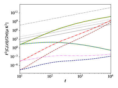
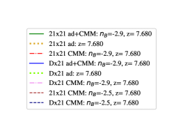
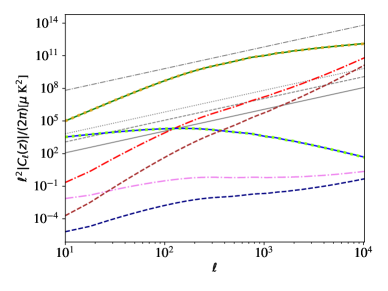
Figure 2: Absolute values of the angular power spectrum of the auto correlation of the 21 cm line signal (21x21) as well as its cross correlation with the CMB Doppler mode (Dx21) as a function of multipole $\ell$ for homogeneous (left) and inhomogeneous reionization (right) for magnetic fields with amplitude $B_{0}=4$ nG and magnetic spectral indices $n_{B}=-2.9$ and $n_{B}=-2.5$ at a reionization redshift $z_{reio}=7.68$. Numerical solutions are shown for the adiabatic mode (ad) and the compensated magnetic mode (CMM) as well as the total (ad+CMM). Also shown are the noise power spectra for LOFAR ( grey, dot-dashed line), SKA1-low (grey, dotted line), SKA1-mid (grey, dashed line) and the optimized configuration SKA1-mid opt (grey, solid line) .

Moreover, using the general expression of Zaldarriaga et al. (2004); Alvarez et al. (2006) for the noise power spectrum,

$$\frac{\ell^{2}N_{\ell}^{21}}{2\pi}=\frac{(130\mu K)^{2}}{N_{month}\Delta\nu_{\rm MHz}}\left[\left(\frac{\ell}{100}\right)\left(\frac{1+z}{10}\right)\left(\frac{D}{1{\rm km}}\right)\left(\frac{10^{3}{\rm m}^{2}{\rm K}^{-1}}{A_{eff}/T_{sys}}\right)\right]^{2}$$ (2.30)

the sensitivities for an observation time of 1.3 months with LOFAR(4,100,61), SKA1-low(300,80,559) and SKA1-mid(770,150,1560) Dewdney (2015) are also included in figure 2. In parentheses are given the specifications of the, already existing (LOFAR) or in the stage of construction (SKAO), radio telescope arrays, namely, the bandwidth in MHz, the baseline in km and the ratio of the effective area over system temperature $A_{eff}/T_{sys}$ in m²/K. For SKA1-mid numerical solutions are also shown for 13 months of observation time as a hypothetical optimized configuration denoted as SKA1-mid opt.

The cross correlation function at multipoles $\ell=120,10^{3}$ and $10^{4}$ is shown in figure 3 as a function of redshift for two different reionization redshifts, namely the bestfit value of the Planck 2018 only data, $z_{reio}=7.68$ (thick lines) and at a higher redshift of $z_{reio}=9$ (thin lines). As can be seen in figure 3 there is a local extremum around the redshift of reionization. The maximal contribution of the cross correlation is found for the adiabatic mode (ad) at the lowest multipole shown, namely, $\ell=120$ which corresponds approximately to the peak in the Doppler mode auto correlation function. This can also be seen in figure 2 where the cross correlation function as a function of multipole $\ell$ is shown at $z_{reio}=7.68$. For the compensated magnetic mode (CMM) the largest contribution of the cross correlation function is found at the largest value, $\ell=10^{4}$, which is due to a local maximum in the linear matter power spectrum generated by the Lorentz term contribution in the baryon velocity evolution equation (e.g., Shaw and Lewis (2010); Kunze (2019, 2021)). Moreover, the largest contribution is found for smaller magnetic field spectral index $n_{B}=-2.9$ which is reflected in the complementary figure 2 showing the evolution of the cross correlation function as a function of $\ell$ at fixed redshift $z=z_{reio}=7.68$.

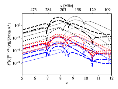
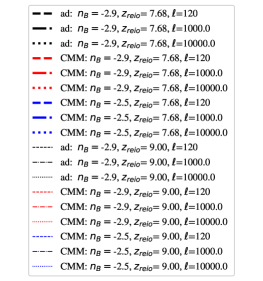
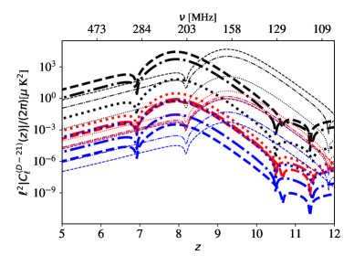
Figure 3: The absolute value of the cross correlation function of the CMB Doppler mode and 21 cm line signal at multipole $\ell=120,10^{3}$ and $\ell=10^{4}$ as a function of redshift for homogeneous (left) and inhomogeneous reionization (right) for magnetic fields with amplitude $B_{0}=4$ nG and magnetic spectral indices $n_{B}=-2.9$ and $n_{B}=-2.5$ at reionization redshifts $z_{reio}=7.68$ (thick lines) and $z_{reio}=9$ (thin lines). Numerical solutions are shown for the adiabatic mode (ad) and the compensated magnetic mode (CMM) .

Comparing the results for homogeneous and inhomogeneous reionization amplitudes are larger for the cross- and auto correlation functions for the latter (cf. figures 2 and 3, left- and right-hand side panels, respectively). This is due to the assumption that the fluctuations in the ionization fraction for the inhomogeneous scenario is directly proportional to the matter power spectrum (cf. equation (2.13)) leading to additional contributions in the auto- and cross correlation angular power spectra, cf. equations (2.12) and (2.29), respectively. In figure 3 the upper horizontal axis shows the frequency of observation of a 21 cm signal corresponding to 1420 MHz originating at redshift $z$, namely, $\nu=1420$ MHz$/(1+z)$.

For the potential observability the signal-over-noise ratio $\frac{S}{N}$ is an important indicator. This can be estimated as Ma et al. (2018); Doré et al. (2004); Adshead and Furlanetto (2008)

$$\left(\frac{S}{N}\right)^{2}=\frac{f_{sky}(2\ell+1)\Delta\ell_{bin}\left(C_{\ell}^{(D-21)}\right)^{2}}{C_{\ell}^{(CMB)}\left(C_{\ell}^{(21-21)}+N_{\ell}^{(21)}\right)+\left(C_{\ell}^{(D-21)}\right)^{2}},$$ (2.31)

where $\Delta\ell_{bin}\simeq 0.46\ell$ is the bin width at a given $\ell$ and $f_{sky}$ the observed sky fraction observed by both the CMB and 21 cm line telescope arrays. Following Ma et al. (2018) $f_{sky}$ is set to $f_{sky}^{CMB,LOFAR}=0.0006$ for CMB and LOFAR observations and $f_{sky}^{CMB,SKA}=0.0024$ for CMB and SKA observations. Also included is the hypothetical optimized configuration and survey design for 13 months of observation and $f_{sky}^{CMB,opt}=1$ denoted as SKA1-mid opt. In figure 4 the signal-over-noise ratio is shown for LOFAR, SKA1-low, SKA1-mid as well as SKA1-mid opt.

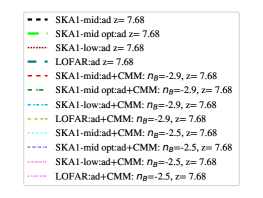
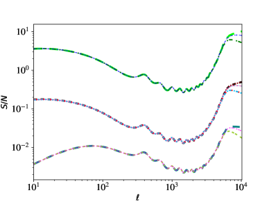
Figure 4: Signal-over-noise ratio of the angular power spectrum of the cross correlation between the CMB Doppler mode and the 21 cm line signal as a function of multipole $\ell$ for homogeneous (left) and inhomogeneous reionization (right) for magnetic fields with amplitude $B_{0}=4$ nG and magnetic spectral indices $n_{B}=-2.9$ and $n_{B}=-2.5$ at reionization redshift $z_{reio}=7.68$. Numerical solutions are shown for the adiabatic mode (ad) and the compensated magnetic mode (CMM) as well as the total (ad+CMM) for LOFAR, SKA1-low, SKA1-mid and SKA1-mid opt.

The signal-over-noise ratio only becomes of ${\cal O}(1)$ for the hypothetical optimized configuration SKA1-mid opt in the case of homogeneous reionization (cf. figure 4, left-hand panel) and $\frac{S}{N}>1$ for inhomogeneous reionization (cf. figure 4, right-hand panel). However, in the latter case it is interesting to note that at high multipoles solutions for different magnetic field parameters are distinguishable. Moreover, even the results for the proposed SKA1-mid configuration are in general not much smaller than one implying that an adjustment of the planned survey and configuration specifications might lead to $\frac{S}{N}\sim 1$. Thus this might open up the possibility to constrain the magnetic field parameters.

It is also interesting to consider the cumulative signal-over-noise ratio defined by $\left(\frac{S}{N}\right)_{cum}$ Ma et al. (2018)

$$\left(\frac{S}{N}\right)_{cum}^{2}(<\ell^{\prime})=\sum_{i}\frac{f_{sky}(2\ell_{i}+1)\Delta\ell_{bin,i}\left(C_{\ell_{i}}^{(D-21)}\right)^{2}}{C_{\ell_{i}}^{(CMB)}\left(C_{\ell_{i}}^{(21-21)}+N_{\ell_{i}}^{(21)}\right)+\left(C_{\ell_{i}}^{(D-21)}\right)^{2}},$$ (2.32)

where $i$ denotes the $ith$ bin with $\ell_{i}$ its central multipole and $\ell^{\prime}$ the maximal multipole implying $\ell_{i}\leq\ell^{\prime}$. In figure 5 the cumulative signal-over-noise ratio as a function of the maximal multipole $\ell^{\prime}$ is shown for LOFAR, SKA1-low, SKA1-mid as well as SKA1-mid opt.

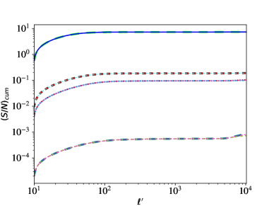
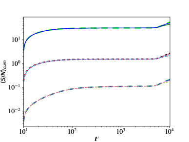
Figure 5: Cumulative signal-over-noise ratio of the angular power spectrum of the cross correlation between the CMB Doppler mode and the 21 cm line signal as a function of the maximal multipole $\ell^{\prime}$ for homogeneous (left) and inhomogeneous reionization (right) for magnetic fields with amplitude $B_{0}=4$ nG and magnetic spectral indices $n_{B}=-2.9$ and $n_{B}=-2.5$ at reionization redshift $z_{reio}=7.68$. Numerical solutions are shown for the adiabatic mode (ad) and the compensated magnetic mode (CMM) as well as the total (ad+CMM) for LOFAR, SKA1-low, SKA1-mid and SKA1-mid opt.

For homogeneous reionization the cumulative signal-over-noise ratio is less than one in all but the case of the SKA1-mid opt configuration where it is of ${\cal O}(10)$ (cf. figure 5 (left-hand side panel)). As can be seen in figure 5 (right-hand side panel) for inhomogeneous reionization for $\ell^{\prime}>20$ configurations of SKA1-low and SKA1-mid have a cumulative signal-over-noise ratio of order one and larger and the SKA1-mid opt configuration has values between 30 and 50 for $\left(\frac{S}{N}\right)_{cum}$. Moreover, there is a distinction between solutions for different magnetic field parameters for large values of the maximal multipole $\ell^{\prime}$.

In figure 6 the signal-over-noise ratio $\left(\frac{S}{N}\right)_{\ell}(z)$ is shown as a function of redshift at fixed different multipoles $\ell=120,10^{3},10^{4}$. The reionization redshift is set to $z_{reio}=7.68$ corresponding to the bestfit value of the Planck 2018 data. $\left(\frac{S}{N}\right)_{\ell}(z)$ is only shown for SKA1-mid and the hypothetical optimized configuration SKA1-mid opt. This is motivated by the previous results. As can be seen in figure 2 the amplitude of the noise angular power spectrum is smallest for the SKA1-mid configurations. In figures 4 and 5 the signal-to-noise ratio as function of $\ell$ at a fixed redshift as well as its cumulative value are largest for the SKA1-mid configurations indicating the best prospects for detection.

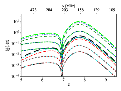
Figure 6: Signal-over-noise ratio of the angular power spectrum of the cross correlation between the CMB Doppler mode and the 21 cm line signal as a function of redshift $z$ for multipoles $\ell=120,10^{3},10^{4}$ for homogeneous (left) and inhomogeneous reionization (right) for magnetic fields with amplitude $B_{0}=4$ nG and magnetic spectral indices $n_{B}=-2.9$ and $n_{B}=-2.5$ at reionization redshift $z_{reio}=7.68$. Numerical solutions are shown for the adiabatic mode (ad) and the compensated magnetic mode (CMM) as well as the total (ad+CMM) for SKA1-mid and SKA1-mid opt.

As can be seen in figure 6 the signal-over-noise ratios indicate a distinction between the pure adiabatic mode and the total adiabatic plus compensated magnetic mode for magnetic field parameters $B_{0}=4$ nG and $n_{B}=-2.9$ and $n_{B}=-2.5$, respectively. In particular, considering the case of inhomogeneous reionization amplifies this separation of curves. Therefore, considering different survey designs might be interesting in order to use the cross correlation between the CMB Doppler mode temperature fluctuations and the 21 cm line brightness fluctuations to constrain parameters of a probable cosmological magnetic field.

III Conclusions

The cross correlation angular power spectrum between the CMB Doppler mode and the 21 cm line signal has been calculated in the presence of a primordial magnetic field assumed to be a random gaussian non helical field. Numerical solutions have been obtained for homogeneous and inhomogeneous reionization for CMB observations and 21 cm line radio telescope configurations and surveys with LOFAR and SKA1-low as well as SKA1-mid. In the signal-over-noise $S/N$ figures also a hypothetical optimized configuration of SKA1-mid has been included. Solutions for $S/N$ have been presented as a function of multipole $\ell$ at fixed redshifts $z$ as well as a function of redshift $z$ at fixed values of multipole $\ell$. For magnetic fields with amplitude $B_{0}=4$ nG and spectral indices $n_{B}=-2.9$ and $n_{B}=-2.5$, respectively, the signal-over-noise ratios resulting from the adiabatic and magnetic mode contributions for inhomogeneous reionization reaches values larger than 1 and in the case of the cumulative signal-over-noise ratio it reaches values between 30 and 50. However, it should be taken into account that these results depend on the particular model of reionization used here. These figures indicate that there might be potentially a possibility for advanced configurations to constrain magnetic field parameters with 21 cm line observations.

IV Acknowledgements

Financial support by Spanish Science Ministry grant PID2021-123703NB-C22 (MCIU/AEI/FEDER, EU) and Basque Government grant IT1628-22 is gratefully acknowledged.

References

- Durrer and Neronov (2013) R. Durrer and A. Neronov, Astron. Astrophys. Rev. 21, 62 (2013), eprint 1303.7121.
- Kandus et al. (2011) A. Kandus, K. E. Kunze, and C. G. Tsagas, Phys.Rept. 505, 1 (2011), eprint 1007.3891.
- Giovannini (2004) M. Giovannini, Phys. Rev. D 70, 123507 (2004), eprint astro-ph/0409594.
- Giovannini and Kunze (2008) M. Giovannini and K. E. Kunze, Phys. Rev. D 78, 023010 (2008), eprint 0804.3380.
- Paoletti et al. (2009) D. Paoletti, F. Finelli, and F. Paci, Mon. Not. Roy. Astron. Soc. 396, 523 (2009), eprint 0811.0230.
- Kahniashvili and Ratra (2005) T. Kahniashvili and B. Ratra, Phys. Rev. D71, 103006 (2005), eprint astro-ph/0503709.
- Shaw and Lewis (2010) J. R. Shaw and A. Lewis, Phys.Rev. D81, 043517 (2010), eprint 0911.2714.
- Kunze (2011) K. E. Kunze, Phys. Rev. D83, 023006 (2011), eprint 1007.3163.
- Shaw and Lewis (2012) J. R. Shaw and A. Lewis, Phys. Rev. D 86, 043510 (2012), eprint 1006.4242.
- Kunze (2012) K. E. Kunze, Phys.Rev. D85, 083004 (2012), eprint 1112.4797.
- Sethi and Subramanian (2005) S. K. Sethi and K. Subramanian, Mon.Not.Roy.Astron.Soc. 356, 778 (2005), eprint astro-ph/0405413.
- Kunze and Komatsu (2015) K. E. Kunze and E. Komatsu, JCAP 1506, 027 (2015), eprint 1501.00142.
- Ade et al. (2016) P. A. R. Ade et al. (Planck), Astron. Astrophys. 594, A19 (2016), eprint 1502.01594.
- Aghanim et al. (2020) N. Aghanim et al. (Planck), Astron. Astrophys. 641, A6 (2020), [Erratum: Astron.Astrophys. 652, C4 (2021)], eprint 1807.06209.
- Furlanetto et al. (2006) S. R. Furlanetto, S. P. Oh, and F. H. Briggs, Phys. Rept. 433, 181 (2006), eprint astro-ph/0608032.
- Loeb and Furlanetto (2013) A. Loeb and S. R. Furlanetto, The First Galaxies in the Universe (Princeton University Press, 2013).
- Kunze (2019) K. E. Kunze, JCAP 2019, 033 (2019), eprint 1805.10943.
- Santos et al. (2010) M. G. Santos, L. Ferramacho, M. B. Silva, A. Amblard, and A. Cooray, Mon. Not. Roy. Astron. Soc. 406, 2421 (2010), eprint 0911.2219.
- Hassan et al. (2016) S. Hassan, R. Davé, K. Finlator, and M. G. Santos, Mon. Not. Roy. Astron. Soc. 457, 1550 (2016), eprint 1510.04280.
- Alvarez et al. (2006) M. A. Alvarez, E. Komatsu, O. Dore, and P. R. Shapiro, Astrophys. J. 647, 840 (2006), eprint astro-ph/0512010.
- Adshead and Furlanetto (2008) P. Adshead and S. Furlanetto, Mon. Not. Roy. Astron. Soc. 384, 291 (2008), eprint 0706.3220.
- Dewdney (2015) P. Dewdney, SKA1 System baseline v2 description 2015-11-04, www.skao.int (2015).
- van Haarlem et al. (2013) M. P. van Haarlem, M. W. Wise, A. W. Gunst, G. Heald, J. P. McKean, J. W. T. Hessels, A. G. de Bruyn, R. Nijboer, J. Swinbank, R. Fallows, et al., Astron. Astrophys. 556, A2 (2013), eprint 1305.3550.
- Kunze (2021) K. E. Kunze, JCAP 11, 044 (2021), eprint 2106.00648.
- Lesgourgues (2011a) J. Lesgourgues (2011a), eprint 1104.2932.
- Blas et al. (2011) D. Blas, J. Lesgourgues, and T. Tram, JCAP 1107, 034 (2011), eprint 1104.2933.
- Lesgourgues (2011b) J. Lesgourgues (2011b), eprint 1104.2934.
- Lesgourgues and Tram (2011) J. Lesgourgues and T. Tram, JCAP 1109, 032 (2011), eprint 1104.2935.
- Lesgourgues and Tram (2014) J. Lesgourgues and T. Tram, JCAP 1409, 032 (2014), eprint 1312.2697.
- Subramanian and Barrow (1998) K. Subramanian and J. D. Barrow, Phys. Rev. D58, 083502 (1998), eprint astro-ph/9712083.
- Jedamzik et al. (1998) K. Jedamzik, V. Katalinic, and A. V. Olinto, Phys. Rev. D57, 3264 (1998), eprint astro-ph/9606080.
- Zaldarriaga et al. (2004) M. Zaldarriaga, S. R. Furlanetto, and L. Hernquist, Astrophys. J. 608, 622 (2004), eprint astro-ph/0311514.
- Kaiser (1987) N. Kaiser, Mon. Not. Roy. Astron. Soc. 227, 1 (1987).
- Shaw and Lewis (2008) J. Shaw and A. Lewis, Phys. Rev. D 78, 103512 (2008), eprint 0808.1724.
- Kunze (2014) K. E. Kunze, Phys. Rev. D 89, 103016 (2014), eprint 1312.5630.
- Kodama and Sasaki (1984) H. Kodama and M. Sasaki, Progress of Theoretical Physics Supplement 78, 1 (1984).
- Hu and White (1997) W. Hu and M. J. White, Phys.Rev. D56, 596 (1997), eprint astro-ph/9702170.
- Furlanetto and Oh (2005) S. R. Furlanetto and S. P. Oh, Mon. Not. Roy. Astron. Soc. 363, 1031 (2005), eprint astro-ph/0505065.
- Basilakos et al. (2008) S. Basilakos, M. Plionis, and C. Ragone-Figueroa, Astrophys.J. 678, 627 (2008), eprint 0801.3889.
- Papageorgiou et al. (2012) A. Papageorgiou, M. Plionis, S. Basilakos, and C. Ragone-Figueroa, Mon.Not.Roy.Astron.Soc. 422, 106 (2012), eprint 1201.4878.
- Abramowitz and Stegun (1968) M. Abramowitz and I. A. Stegun, Handbook of mathematical functions with formulas, graphs and mathematical tables (Dover, 1968).
- Villaescusa-Navarro et al. (2018) F. Villaescusa-Navarro, S. Genel, E. Castorina, A. Obuljen, D. N. Spergel, L. Hernquist, D. Nelson, I. P. Carucci, A. Pillepich, F. Marinacci, et al., Astrophys.J. 866, 135 (2018), eprint 1804.09180.
- Nusser and Tiwari (2015) A. Nusser and P. Tiwari, Astrophys.J. 812, 85 (2015), eprint 1505.06817.
- Shen et al. (2009) Y. Shen, M. A. Strauss, N. P. Ross, P. B. Hall, Y.-T. Lin, G. T. Richards, D. P. Schneider, D. H. Weinberg, A. J. Connolly, X. Fan, et al., Astrophys.J. 697, 1656 (2009), eprint 0810.4144.
- Marín et al. (2013) F. A. Marín, C. Blake, G. B. Poole, C. K. McBride, S. Brough, M. Colless, C. Contreras, W. Couch, D. J. Croton, S. Croom, et al., Mon. Not. Roy. Astron. Soc. 432, 2654 (2013), eprint 1303.6644.
- Vishniac (1987) E. T. Vishniac, Astrophys.J. 322, 597 (1987).
- Ostriker and Vishniac (1986) J. Ostriker and E. Vishniac, Astrophys.J. 306, L51 (1986).
- Hu (2000) W. Hu, Astrophys.J. 529, 12 (2000), eprint astro-ph/9907103.
- Hu and White (1996) W. Hu and M. J. White, Astron.Astrophys. 315, 33 (1996), eprint astro-ph/9507060.
- Gradshteyn et al. (2000) I. S. Gradshteyn, I. M. Ryzhik, A. Jeffrey, and D. Zwillinger, Table of Integrals, Series, and Products (Academic Press, 2000).
- Ma et al. (2018) Q. Ma, K. Helgason, E. Komatsu, B. Ciardi, and A. Ferrara, Mon. Not. Roy. Astron. Soc. 476, 4025 (2018), eprint 1712.05305.
- Doré et al. (2004) O. Doré, J. F. Hennawi, and D. N. Spergel, Astrophys.J. 606, 46 (2004), eprint astro-ph/0309337.