Redeveloping a CLEAN Deconvolution Algorithm for Scatter-Broadened Radio Pulsar Signals

Abstract

Broadband radio waves emitted from pulsars are distorted and delayed as they propagate toward the Earth due to interactions with the free electrons that compose the interstellar medium, with lower radio frequencies being more impacted than higher frequencies. Multipath propagation in the interstellar medium results in both later times of arrival for the lower frequencies and causes the observed pulse to arrive with a broadened tail described via the pulse broadening function. We employ the CLEAN deconvolution technique to recover both the intrinsic pulse shape and pulse broadening function. This work expands upon previous descriptions of CLEAN deconvolution used in pulse broadening analyses by parameterizing the efficacy on simulated data and developing a suite of tests to establish which of a set of figures of merit lead to an automatic and consistent determination of the scattering timescale and its uncertainty. We compare our algorithm to simulations performed on cyclic spectroscopy estimates of the scattering timescale. We test our improved algorithm on the highly scattered millisecond pulsar J1903+0327, showing the scattering timescale to change over years, consistent with estimates of the refractive timescale of the pulsar.

1 Introduction

Radio pulsars provide unique probes of the ionized interstellar medium (ISM) and allow us to gain insight into its structure and variability by modeling the effects of the delays and distortions on the emitted radio pulses as observed at the Earth (Lorimer & Kramer, 2004). While delays due to dispersion are routinely modeled in pulsar timing experiments (e.g., Verbiest et al., 2016), distortions due to multipath propagation are not and it can be difficult to do so (Shannon & Cordes, 2017). Determining the distortion level is difficult due to both the intrinsic pulse shape and the underlying geometry and spectrum of the turbulent medium being unknown (Cordes et al., 1986; Cordes & Rickett, 1998), and the time and path-dependent variations in the observed pulse broadening function (PBF; Williamson, 1972). Not only can separating these effects yield important insights into the nature of the ionized ISM but also provide proper pulse profile impact mitigation for pulsars used in precision timing experiments such as low-frequency gravitational wave detectors (Stinebring, 2013).

CLEAN deconvolution, originally developed for radio interferometric imaging (Högbom, 1974), was applied to radio pulses in Bhat et al. (2003) to recover both the pulse broadening (scattering) timescale $\tau_{\rm d}$ and the intrinsic shape simultaneously via the use of an assumed PBF. Unlike in synthesis imaging where the positions of the array elements are known while the sky brightness distribution is not, neither the analogous PBF nor intrinsic pulse shape, respectively, are known. Bhat et al. (2003) introduced figures of merit to iteratively test trial values of $\tau_{\rm d}$ under an assumed PBF, demonstrating variation in the rebuilt intrinsic pulses for PSR J1852+0031 for different PBFs and application to several other pulsars.

We expand upon the CLEAN deconvolution algorithm presented in Bhat et al. (2003) to prepare for automated deployment on data sets of significantly more pulsars. In this work, we primarily focus on the broadening effects of the ISM and recovering $\tau_{\rm d}$ with the intention of applying the algorithm to the multi-frequency profiles of pulsars distributed throughout the galaxy to understand both the bulk properties of the turbulence in the ISM and specific unique lines of sight. Understanding these properties inform priors on pulsar timing arrays and other high-precision pulsar timing experiments in which scattering biases estimates of the arrival times (Lentati et al., 2017). This work is the first of several papers on robust method development and deployment on real data from a larger selection of pulsar observations.

In §2, we describe the CLEAN deconvolution method as presented and expanded upon the work in Bhat et al. (2003). In §3, we perform systematic tests on simulated data, demonstrating the level of recall in the input $\tau_{\rm d}$ values and quantifying our uncertainties in the estimates. We also compare our results with the cyclic spectroscopy (CS) deconvolution technique and discuss the tradeoff of limitations in our method with the extensive computational complexity of the CS method. Finally, we apply our method to PSR J1903+0327 in §4 and discuss our future directions in §5.

2 The CLEAN Deconvolution Algorithm

CLEAN deconvolution for radio pulsars exploits the one-dimensional nature of pulsar profiles and differs from traditional CLEAN approaches where the instrumental response function is known. The analogous function in this work, the PBF, must be assumed from a priori models. Bhat et al. (2003) developed a method that can both determine the pulse broadening timescale $\tau_{\rm d}$ and recover the intrinsic pulse from observational pulsar profile data via the employment of a CLEAN deconvolution algorithm and figures of merit (FOMs). CLEAN can be applied using different models of the PBF of the ISM, making it a broadly encompassing method. In this work, we assumed the PBF for the commonly-used thin-screen approximation for the ISM’s geometry.

Bhat et al. (2003) described the CLEAN algorithm for use in the deconvolution of radio pulsar pulses, along with the development of five FOMs used to determine the correct broadening timescale from a set of test values. In this section, we discuss the algorithm both as originally described and how the algorithm has been redeveloped for this work.

2.1 Modeling the Observed Pulse Profile

We assumed the observed pulse $y(t)$ to result from the convolution of the intrinsic pulse $x(t)$, the PBF $g(t)$, and the instrumental response function $r(t)$, given by

$$y(t)=x(t)\otimes g(t)\otimes r(t).$$ (1)

We simulated our intrinsic pulse $x(t)$ as a normalized, single-peaked Gaussian shape, which minimizes the asymmetry of the rebuilt pulse and provides a baseline comparison against the use of the FOM $\Gamma$ discussed later in Section 2.3.1.

The PBF for the ISM is commonly modeled as a thin screen (Cordes & Rickett, 1998) for simplicity. The thin-screen approximation simplifies calculations, separating out the physical turbulent processes from the geometry of the intervening gas, and in the case of the PBF, simplifies the form as well; the thin-screen model works reasonably well for lines of sight with a single overdense region. We used this model in our work, given by

$$g(t|\tau_{\rm d})=\frac{1}{\tau_{\rm d}}\exp\left(-\frac{t}{\tau_{\rm d}}\right)U(t),$$ (2)

where $U(t)$ is the Heaviside step function.

Lastly, the instrumental response function denoted as $r(t)$ determines the resolution of the observed data. We assumed a delta function as an approximation for the instrumental response function with a width of one phase bin.

2.2 CLEAN Deconvolution

CLEAN iteratively subtracts replicated components from an observed pulse until the residual structure falls below the root mean squared (rms) of the off-pulse noise. As we do not know the value of $\tau_{\rm d}$ a priori, this iterative subtraction process is repeated for a range of test $\tau_{\rm d}$ values, with the assumed correct $\tau_{\rm d}$ chosen using FOMs. For the purposes of the algorithm, we treat $\tau_{\rm d}$ to be measured in time-bin resolution units as measured across the folded pulse’s phase with $N_{\phi}$ total bins. We step through our CLEAN deconvolution process below.

1. CLEAN Component Creation: We first identify the location of the maximum of the deconstructed pulse after the $i$-th iteration, $t_{i}\equiv\operatorname*{argmax}\left[y_{i}(t)\right]$; our first iteration begins with the originally observed pulse $y_{0}(t)$. Each CLEAN component (CC) $y_{c}(t|t_{i})$ starts with a delta function $\delta(t-t_{i})$ at the location of the maximum of the observed pulse, $\max\left[y_{i}(t)\right]$ multiplied by the loop gain value $\gamma$, i.e.,

   $$y_{c}(t|t_{i})=\gamma\left\{\max\left[y_{i}(t)\right]\right\}\delta(t-t_{i})\equiv C_{i}\delta(t-t_{i}).$$ (3)

   Smaller loop gains result in a greater number of iterations before the stopping criterion is met but allow for finer intrinsic features to be resolved (Högbom, 1974); in this work, we used $\gamma=0.05$.

2. Iterative Subtraction off the Main Pulse: After we construct $y_{c}(t|t_{i})$, we convolve the CC with the instrumental response function $r(t)$ and the PBF with a given test $\tau_{\rm d}$, and then subtract this shape from the $i$-th iteration pulse. The change in the profile at each iteration is described as

   $$\Delta y_{i}(t)=y_{i}(t)-\left\{y_{c}(t|t_{i})\otimes\left[g(t|\tau_{\rm d})\otimes r(t)\right]\right\}$$ (4)

   with $y(t_{i})$ as the input pulse profile to the $i$-th iteration. The CCs are then iteratively subtracted off the main pulse, with the resulting subtracted profile becoming the pulse profile for the next CLEAN iteration so that

   $$y_{i+1}(t)=\Delta y_{i}(t).$$ (5)

3. Termination of CLEAN Algorithm: The CLEAN algorithm is terminated when the maximum of the input pulse profile falls below the rms of the off-pulse noise, i.e., $\max\left[y_{i}(t)\right]\leq\sigma_{\rm off}$.

The CLEAN algorithm above will provide the list of CCs along with the residual noise. The CCs can be used to reconstruct the intrinsic pulse shape, but for the purposes of this work, our final goal was to determine $\tau_{\rm d}$. The algorithm can run with any input value of $\tau_{\rm d}$, therefore our iterative method is repeated with different trial $\tau_{\rm d}$, from which we derived FOMs based on the reconstructed intrinsic pulse shape and the residual noise that resulted from each trial $\tau_{\rm d}$.

Figure 1: Summary of FOMs used in this work, for a pulse with simulated full-width at half maximum of 100 phase bin units, input $\tau_{\rm d}=50$ phase bins, and $\mathrm{S/N}=100$. We tested $\tau_{\rm d}$ values ranging from 25 to 75 bin units with a step size of one. Panel 1 shows the number of data points within a 3$\sigma$ level of the noise FOM, panel 2 shows the root mean squared FOM, panel 3 shows the skewness FOM, panel 4 shows the positivity FOM, panel 5 shows the combined skewness and positivity FOM, and panel 6 shows the number of iterations FOM.

2.3 Figures of Merit

We employed six FOMs as follows: a measure of positivity of the residual noise ($f_{\rm r}$), a measure of skewness of the recovered intrinsic pulse ($\Gamma$), a count of the on-pulse-region residual points below the off-pulse noise level ($N_{\rm f}$/$N_{\rm\phi}$), a measure of the ratio of the rms of the residual noise to the off-pulse noise rms ($\sigma_{\rm offc}$/$\sigma_{\rm off}$), a measure of the combined positivity and skewness measure ($f_{\rm c}$), and a count of the number of CLEAN components each test $\tau_{\rm d}$ uses before the peak of the profile falls below the noise level ($N_{\rm iter}$). All except the last are described in Bhat et al. (2003). These six FOMs fall into three broad categories: figures based on the rebuilt intrinsic pulse, figures based on the residual noise after the CLEAN algorithm terminates, and a figure based on the number of CLEAN components generated before the algorithm terminates. We describe the FOMs grouped into these three categories in the sections below.

In Figure 1, we see the ideal result of the use of six FOMs and the methods for determining the “correct” $\tau_{\rm d}$.

2.3.1 FOM Measuring the Shape of the Rebuilt Intrinsic Pulse

We examine the CC amplitudes $C_{i}$ and locations $t_{i}$ found during the CLEAN process (e.g., see Eq. 3) to compute the $\Gamma$ FOM. In our simulations, we created intrinsic pulses that are symmetric Gaussians, and therefore the correct rebuilt pulse should always be a perfectly symmetric Gaussian if the correct $\tau_{\rm d}$ is used. In reality, intrinsic pulses may not be perfectly symmetric, and we discuss these implications in §5.

The $\Gamma$ of the rebuilt pulses is calculated for each test $\tau_{\rm d}$ by computing the third standardized moment

$$\Gamma=\frac{\left<t^{3}\right>}{\left<t^{2}\right>^{3/2}},$$ (6)

where $\left<t^{n}\right>$ is

$$\left<t^{n}\right>=\frac{\sum_{i=1}^{n_{c}}(t_{i}-\bar{t})^{n}C_{i}}{\sum_{i=1}^{n_{c}}C_{i}}$$ (7)

and $\bar{t}$ is

$$\bar{t}=\frac{\sum_{i=1}^{n_{c}}t_{i}C_{i}}{\sum_{i=1}^{n_{c}}C_{i}}.$$ (8)

The resulting $\Gamma$ is ideally represented by the example in panel 3 of Figure 1, where the sharp fall-off point represents the general location of the correct $\tau_{\rm d}$.

2.3.2 FOMs Based on the Residual Noise

Three of our FOMs are built from measures of the residual noise after the completion of the CLEAN algorithm. We will also discuss a FOM that combines one of these FOMs (positivity) with the $\Gamma$ FOM discussed previously – this is an important FOM as described in Bhat et al. (2003).

The residual noise is one of the end products of the CLEAN deconvolution process. A test $\tau_{\rm d}$ that is larger than the correct value of $\tau_{\rm d}$ results in a progressively larger over-subtraction as shown in Figure 2. If the test $\tau_{\rm d}$ is smaller than the correct value, it results in an unremoved noise floor in the baseline, again see Figure 2.

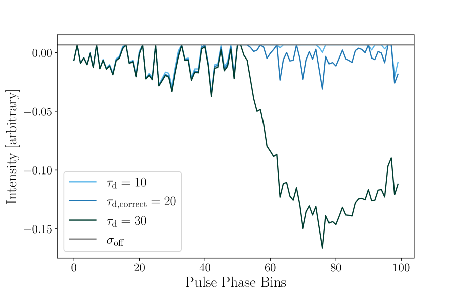
Figure 2: The residual noise left over after the CLEAN algorithm terminates for three test $\tau_{\rm d}$ values, 10, 20, and 30 bins, where 20 is the simulated value. These time series are representative of the residuals used to calculate multiple FOMs. We can see the under- and over-subtraction for test $\tau_{\rm d}$ values that are smaller than or larger than the true $\tau_{\rm d}$, respectively.

We can first calculate the rms of the residual noise

$$\sigma_{\rm offc}=\frac{1}{N_{\phi}}\sum_{j=1}^{N_{\phi}}[\Delta y_{i}(t_{j}|\tau_{\rm d})]^{2},$$ (9)

in comparison to the rms of the off-pulse region, $\sigma_{\rm off}$, where this ratio $\sigma_{\rm offc}/\sigma_{\rm off}$ will grow whenever over- or under-subtraction is performed and should otherwise approach a value of 1 for the appropriate subtraction. This is roughly equivalent to the single metric used to automatically determine $\tau_{\rm d}$ used in Tsai et al. (2017) for multi-frequency data from 347 pulsars.

Beyond the rms, we can count the total number of residual noise points $N_{\rm f}$ within a certain threshold level (we chose $3\sigma_{\rm off}$) of the noise that satisfies the condition

$$|y_{i}-y_{\mathrm{off}}|\leq 3\sigma_{\mathrm{off}}.$$ (10)

As seen in Figure 2, for under-subtraction we expect all of the points to satisfy the condition and so the ratio $N_{\rm f}/N_{\phi}=1$, but the ratio will drop as over-subtraction occurs.

Besides these two metrics which measure deviations away from the rms noise, we also wish to enforce non-negativity of the residual profile since we know pulsar signals must be above the baseline noise. A $f_{\rm r}$ FOM was defined by Bhat et al. (2003) in terms of a sum over the $N_{\phi}$ bins of the residual noise,

$$f_{\rm r}=\frac{1}{N_{\phi}\sigma_{\mathrm{off}}^{2}}\sum_{j=1}^{N_{\phi}}[\Delta y_{i}(t_{j}|\tau_{\rm d})]^{2}.$$ (11)

If $\Delta y_{i}(t)$ is Gaussian white noise with rms equal to $\sigma_{\rm off}$, then as with the previous FOM, we would expect $f_{\rm r}\approx 1$, while over-subtraction would force the sum to increase well beyond 1.

Bhat et al. (2003) defined the $f_{\rm c}$ FOM, equally weighting the rebuilt intrinsic pulse shape and the residual noise by

$$f_{\rm c}=\frac{\Gamma+f_{\rm r}}{2},$$ (12)

thus providing higher confidence in test $\tau_{\rm d}$ values with favorable values of both skewness and positivity. The typical shape of this FOM is shown in panel 5 of Figure 1.

2.3.3 FOM Measuring the Number of Iterations Performed

We developed this FOM to more directly measure the fit of the re-convolved CCs broadening tails to the broadening of the observed pulse. As the amplitude for re-convolved CCs with larger broadening tails is smaller than those with smaller broadening tails (due to the normalization in Eq. 2), we expect a general increase in the number of iterations needed to deconvolve the observed pulse. Similarly, when re-convolved CCs with smaller broadening tails are subtracted from a pulse with a larger true broadening tail, more iterations will be required. However, when the CCs are convolved with the correct value of $\tau_{\rm d}$, neither under nor over-subtraction occurs, resulting in fewer iterations being needed. Therefore, we expect a dip in our FOM around the correct value of $\tau_{\rm d}$.

2.4 Automating the Choice of the Correct $\tau_{\rm d}$ Value

These FOMs were originally constructed to pinpoint the correct value of $\tau_{\rm d}$ by eye. This approach is impractical for large data sets, so we automated this process. We found that the simple approach of computing the numerical third derivative of each function with respect to $\tau_{\rm d}$ and finding the maximum has yielded good results, though the exact recall depends on both the value of $\tau_{\rm d}$ and the pulse S/N. More complicated algorithms will be employed in future works but the systematic error introduced by this choice is small in comparison to other noise sources, as shown next, so we opted to use it.

3 Automated Algorithm Performance

In this section, we will discuss the performance of our automated CLEAN method. An in-depth description of our redeveloped CLEAN algorithm in Python, as well as notes on how to use the open source versions available on https://zenodo.org/badge/latestdoi/524167339, can be found in Young (2022).

We wished to robustly quantify the “correctness” of our $\tau_{\rm d}$ estimates in simulated data so that we could automatically assign uncertainties to our estimates on real data. To that end, we simulated multiple data sets with different input parameters to determine how these will affect the recall. Ideally, as in Dolch et al. (2021) for the cyclic spectroscopy (CS) algorithm, only the S/N and $\tau_{\rm d}$ of a profile should affect the recall accuracy of our CLEAN deconvolution, though we tested several other parameters as well.

To quantify the algorithm’s performance, we computed a measure of the fractional average error bar. Within this work, the values returned for each FOMs were given the same weight when calculating our error bars, which is defined as the fraction of the returned $\tau_{\rm d}$ to the correct injected $\tau_{\rm d}$. Our fractional average error bars are defined as

$$\epsilon_{\rm ave}=1-\frac{1}{N_{\rm runs}}\sum_{i=1}^{N_{\rm runs}}\left(\frac{\epsilon_{i}}{\tau_{\rm d}N_{\rm FOM}}\right)$$ (13)

where $N_{\rm runs}$ is the number of simulations for a given data set, $N_{\rm FOM}=6$ is the number of FOMs used, and $\epsilon_{i}$, for readability, is defined as an unweighted sum of the $\tau_{\rm d}$ values returned by our FOMs for each run ($i=1\dots N_{\rm runs}$),

$$\epsilon_{i}={\tau_{\frac{N_{\rm f}}{{N_{\phi}}}}+\tau_{\frac{\sigma_{\rm offc}}{\sigma_{\rm off}}}+\tau_{\Gamma}+\tau_{f_{\rm r}}+\tau_{f_{\rm c}}+\tau_{N_{\rm iter}}}.$$ (14)

3.1 Testing the Impact of S/N and $\tau_{\rm d}$ on Recall

We first tested how CLEAN performs based on different injected pulse S/N and $\tau_{\rm d}$ combinations. We simulated data sets using several of the characteristics of PSR B1937+21 (the first-known millisecond pulsar and a known scattered source) as follows; these parameters are also shown in Table 2. PSR B1937+21 has a spin period of 1.557 ms and a full-width at half maximum (FWHM) of 38.2 $\mu$s (Manchester et al., 2013). To reduce computing time, we used different numbers of phase bins depending on the injected $\tau_{\rm d}$ value as shown in Table 2; we show in the next subsection that there is minimal impact in the recovery of $\tau_{\rm d}$ depending on the phase resolution of the pulses so long as the scattering tails are resolved. For each of our runs, we tested across 100 equally-spaced $\tau_{\rm d}$ steps between 0.5 and 1.5 times the injected $\tau_{\rm d,correct}$. For each S/N-$\tau_{\rm d}$ pair, we simulated and ran CLEAN on 60 pulse shapes.

We choose our S/N-$\tau_{\rm d}$ values in the same style as Dolch et al. (2021) to more directly compare our CLEAN deconvolution method with the CS algorithm. While CLEAN works on an averaged pulse profile, CS uses raw voltage data prior to folding to recover the full impulse response function, making the latter more computationally intensive (though assuming no specific PBF). These methods are therefore difficult to directly compare, but we can expect to see improved performance for both methods as either S/N or $\tau_{\rm d}$ increase.

Indeed, after running our simulations, we see this expected behavior in Figure 3, where darker colors indicate better recovery of $\tau_{\rm d}$, which matches what is seen in Dolch et al. (2021) for CS. The numerical values shown in Figure 3 are in terms of the percentage of the correct $\tau_{\rm d}$, given by $\epsilon_{\rm ave}$.

Table 1: Automated Algorithm Simulation Parameters

Parameter	Value
Spin period	1.557 ms
Pulse FWHM	38.2 $\mu$s
$N_{\phi}$ for $\tau_{\rm d}=1,2,4~{}\mu\mathrm{s}$	2048
$N_{\phi}$ for $\tau_{\rm d}=8,16,32~{}\mu\mathrm{s}$	1024
$N_{\phi}$ for $\tau_{\rm d}=64,128,256~{}\mu\mathrm{s}$	512
Test $\tau_{\rm d}$ range	(0.5$\tau_{\rm d,correct}$ – 1.5$\tau_{\rm d,correct}$)
Number of steps in test $\tau_{\rm d}$ array	100

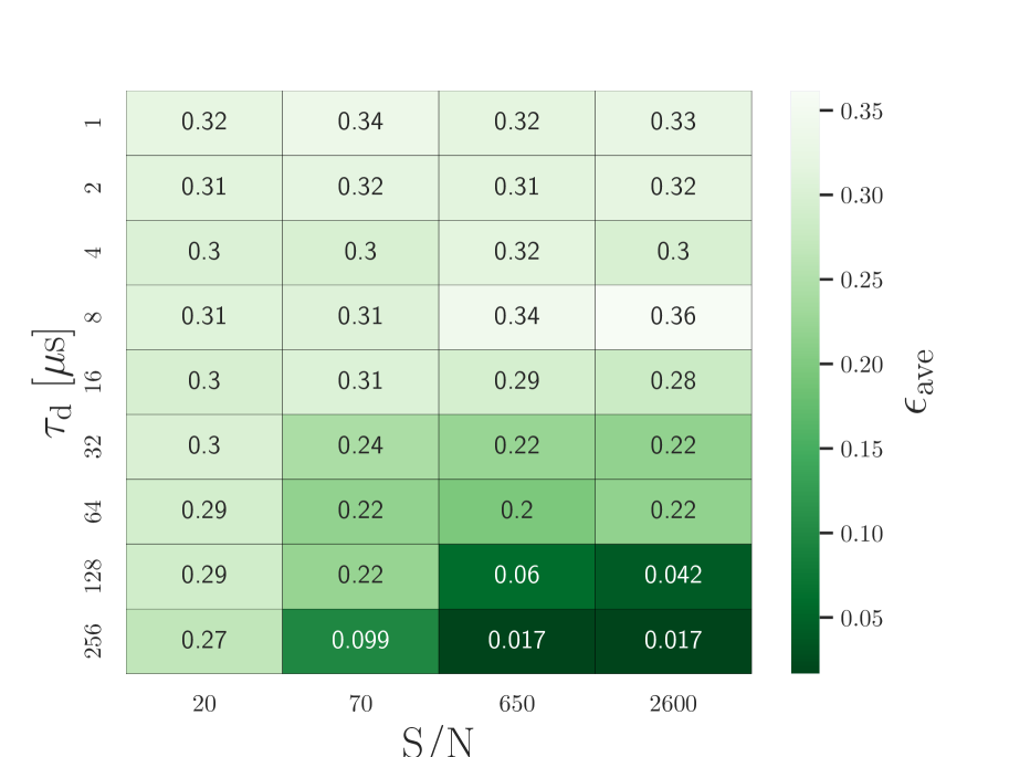
Figure 3: Average recall error bars for CLEAN deconvolution in the same style as Figure 5 from Dolch et al. (2021). This plot gives an encompassing overview of the performance of the CLEAN algorithm by returning the average size of the error bars with each S/N and $\tau_{\rm d}$ pair. As smaller error bars indicate better performance, CLEAN performs better on simulated data with larger values of both S/N and $\tau_{\rm d}$.

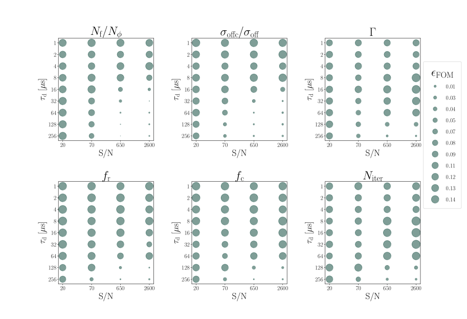
Figure 4: Overview of the relative performance for each FOM. Smaller circles indicate smaller error bars or better performance of the FOMs on simulated data. These factional averages were computed as described in Equation 13, with $\epsilon_{i}$ being composed of the $\tau_{\rm d}$ returned by only one FOM instead of an unweighted sum of all returned $\tau_{\rm d}$ values. These values are labeled as $\epsilon_{\rm FOM}$ in this plot. In general, we see better performance for higher values of $\tau_{\rm d}$ and S/N. Interestingly, the $N_{\rm f}$/$N_{\rm\phi}$ and $\sigma_{\rm offc}$/$\sigma_{\rm off}$ FOM appear to perform better than the $f_{\rm r}$ and the $\Gamma$ FOMs which were highlighted in the Bhat et al. (2003) paper.

In Figure 4, we show how well each individual FOM performs, with each panel showing the recovery over the full range of S/N-$\tau_{\rm d}$ pairs. Smaller dots indicate smaller error bars, and thus a more accurate performance. Poor performance from one FOM will impact our averaged recall, as an unweighted average is currently employed. We see that in general, the performance of each FOM improved with higher S/N or $\tau_{\rm d}$ like the average, though not all behave equally. For example, the $N_{\rm f}/N_{\phi}$ and $\sigma_{\rm offc}/\sigma_{\rm off}$ appear to perform better at somewhat lower $\tau_{\rm d}$ than the other FOMs. While the skewness $\Gamma$ does not perform as well at the high S/N-$\tau_{\rm d}$ end, it does perform marginally better than the previously mentioned two FOMs otherwise. In future works, we will explore developing weights for each FOM in constructing the average $\epsilon_{\rm ave}$ to improve the average accuracy of the algorithm.

3.2 Testing Secondary Parameter Contributions to Recall Error

While we assumed the main contributors to the effectiveness of our algorithm to be our primary parameters, $\mathrm{S/N}$ and $\tau_{\rm d}$, we wanted to ensure that secondary parameters were not significant contributors to our recall error. We created a small-scale parameterization set via simulation of a base pulse profile with $\tau_{\rm d}=256$ bins and $\mathrm{S/N}=2600$. We chose very large values for both $\tau_{\rm d}$ and S/N as the method was able to reliably recall the correct $\tau_{\rm d}$ for large $\tau_{\rm d}$ and S/N values (see Section 3.2). This set was used to determine how the number of bins in our observation, the FWHM of the intrinsic pulse, and the user-defined step size and range of the test $\tau_{\rm d}$ array affected the algorithm’s performance. Additionally, our previous data set assumed an intrinsic pulse with similar parameters to B1937+21 only. Therefore, an additional motivation for probing these secondary parameters was to determine if we can extrapolate our results to observations of other pulsars with varying FWHMs and numbers of phase bins.

For these parameterization runs we used the base values shown in the second column of Table 2 and iterated over the values shown in the third column. We run 20 simulations for each variation, which gave insight into these parameters’ contribution to our recall and allowed for exploration into the expected larger contributions of $\tau_{\rm d}$ and S/N to the recall error.

Table 2: Secondary Parameters Tested

Parameter	Base Value	Values
Number of phase bins	256	$\left\{128,256,512,1024,2048\right\}$
FWHM	$\frac{1}{8}N_{\phi}$	[$\frac{1}{64}$, $\frac{1}{32}$, $\frac{1}{16},\frac{1}{8},\frac{1}{4},\frac{1}{2}$]$N_{\phi}$
Range of $\tau_{\rm d}$	(0.5 $\tau_{\rm d,correct}$ – 1.5 $\tau_{\rm d,correct}$)	(0.1 $\tau_{\rm d,correct}$ – $\tau_{\rm d,correct}$), (0.1 $\tau_{\rm d,correct}$ – 2.0 $\tau_{\rm d,correct}$),
		(0.4 $\tau_{\rm d,correct}$ – 1.6$\tau_{\rm d,correct}$), (0.5 $\tau_{\rm d,correct}$ – 1.5 $\tau_{\rm d,correct}$)
Number of steps in $\tau_{\rm d}$ array	100	[10, 20, 50, 100, 200]

As many pulse profiles are recorded with a different number of phase bins (see e.g., Lorimer et al., 1997), we tested to see how the phase resolution of the observation affected our recall. We simulated data sets with $N_{\phi}$ ranging from 128 to 2048. In Figure 5, we see good agreement between the individual recall values for each run and the averages varying within 10%. Thus, the minor variations in the average recalls could be explained by our limited number of runs resulting in incomplete coverage of the algorithm’s performance and we therefore assumed that the number of bins in the observed pulse profile was not a significant contributor to our total recall.

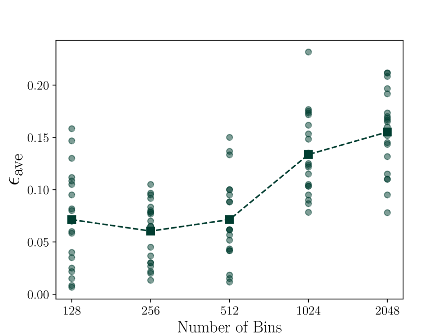
Figure 5: Results of parameterization runs with changing number of phase bins. The y-axis shows the fractional average error bar size across 20 simulations for each bin value. The average recall error is denoted by the fully opaque green squares connected by the dashed line. The lighter circles indicate the recall error from each run. The average error bars range within 10$\%$.

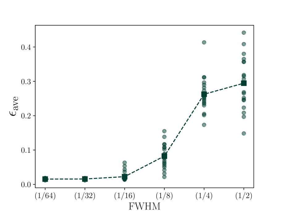
Figure 6: Results of parameterization runs with changing values of the FWHM of the intrinsic pulse, as a fraction of the observation length. We see for FWHMs less than $1/4$, the fractional average error bar changes less than 10%, with the $\epsilon_{\rm ave}$ change still under 30% for the FWHM being $1/2$ the observation window. This effect has been seen with the CS approach as well.

Results of testing how the FWHM of the intrinsic pulse affected our recall are shown in Figure 6, and reveal a large, though not unexpected, range in $\epsilon_{\rm ave}$ between the FWHMs tested. As the FWHM increases, the pulse takes up an increasing fraction of the observation window, thus making the CLEAN cutoff criterion of falling below the off-pulse noise level less effective. This result is corroborated by the findings of Jones et al. (2013) when they found the CS method to be less effective on wider pulses.

In Figure 7, we see the contribution of the number of steps or interchangeably the step size of the test $\tau_{\rm d}$ array to our recall error. We included in this analysis a correction factor of $\Delta\tau_{\rm d}/2$, the largest base error induced due to large step sizes resulting in the correct $\tau_{\rm d}$ not being directly tested. For example, if the correct $\tau_{\rm d}$ is 10.5 $\mu\mathrm{s}$, and our test $\tau_{\rm d}$ array only samples every $\Delta\tau_{\rm d}=1\mu\mathrm{s}$, an error of 0.5 $\mu\mathrm{s}$ will be introduced, thus, we added this factor of $\Delta\tau_{\rm d}/2$ to our $\epsilon_{\rm ave}$ to more conservatively estimate our uncertainties. The fractional average error bars returned vary within 5%, therefore we concluded that the number of steps in the test $\tau_{\rm d}$ array was not a large contributor to the overall recall error.

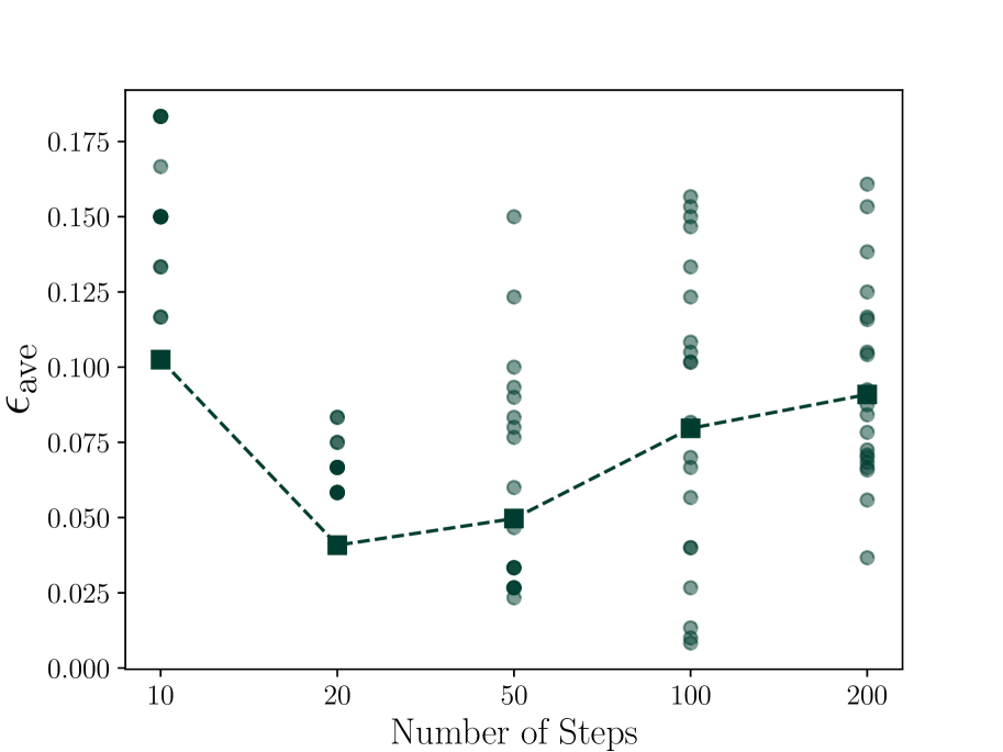
Figure 7: Results of parameterization runs with changing numbers of steps in the test $\tau_{\rm d}$ ranges. Although there is some range in the average errors returned, all values agree within $\approx$5%.

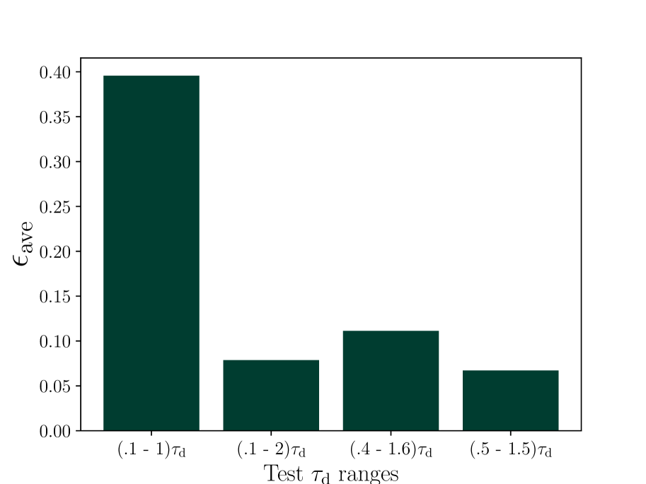
Figure 8: Results of parameterization runs with changing ranges of test $\tau_{\rm d}$ iterated over. We see that as long as the correct $\tau_{\rm d}$ is included within the range of test $\tau_{\rm d}$ iterated over, the range of test $\tau_{\rm d}$ was not a large contributor to the overall recall error.

Finally, we parameterized the contribution of the range of test $\tau_{\rm d}$ iterated over to our recall. In Figure 8, we see that ranges that barely included the correct $\tau_{\rm d}$ (second bar) result in poor performance as expected. This results from the shapes of the FOMs not being fully covered over the correct injected $\tau_{\rm d}$. Other ranges that include the correct $\tau_{\rm d}$ have recalls within about 5% of each other, even when the ranges iterated over are much larger. Therefore, while more computationally intensive, we recommend running CLEAN over a large range of $\tau_{\rm d}$ values to ensure the best estimate is chosen.

With the results of these runs, we see that these secondary effects have some small impact at large S/N and $\tau_{\rm d}$, but otherwise the most prominent influences on the recall of CLEAN deconvolution are the S/N and $\tau_{\rm d}$ of the data. While there are some variations in the average recall for each of the parameters we tested, the average recalls varied within 10% or less for most tests, with the notable exceptions: large FWHMs and test $\tau_{\rm d}$ range that barely included the correct value of $\tau_{\rm d}$, both expected. We can also conclude that the results using one simulated pulsar can be extrapolated to both simulations of other pulsars and real observational data.

4 Applying CLEAN to PSR J1903+0327

To demonstrate the efficacy of our algorithm, we tested CLEAN on real data from the pulsar J1903+0327. PSR J1903+0327 is a millisecond pulsar that has been monitored by pulsar timing array collaborations such as the North American Nanohertz Observatory for Gravitational Waves (NANOGrav; Arzoumanian et al. 2021) in the effort to detect low-frequency gravitational waves. While these collaborations self-select for pulsars with low amounts of pulse broadening (narrower pulses have higher timing precision), PSR J1903+0327 has some of the most prominent scattering in these data sets, with the broadening tail visible by eye. With over a decade of timing data on this pulsar, we analyzed the lowest-radio-frequency pulses in the NANOGrav 12.5-year data set over time, where broadening is the strongest, to investigate if variations in $\tau_{\rm d}$ are detectable by our algorithm.

We created six summed profiles on which to deploy our CLEAN algorithm, with one profile corresponding to each year from 2012-2017 in our data set. We restricted the frequency band for each observation to 10 MHz centered at 1200 MHz to mitigate additional broadening if frequency-averaging the pulses together to boost S/N. Each summed profile consists of twelve monthly observations summed via cross-correlation. Cross-correlation is used to ensure the peaks of our profiles are properly aligned in time before they are summed, resulting in the highest possible S/N of the summed profile. This process was performed iteratively, with each new profile being cross-correlated with and then added to the summed profile.

The refractive timescale of PSR J1903+0327 is estimated to be between 1 and 2 years (Geiger & Lam, 2022). Therefore, summing across one year of observations is consistent with the PBF remaining unchanged across this time span. To further increase the S/N values for each profile, we used different Savitzky-Golay filters to smooth the resulting summed profile to the desired S/N level. In Figure 9, we see an example of this summed and smoothed pulse profile.

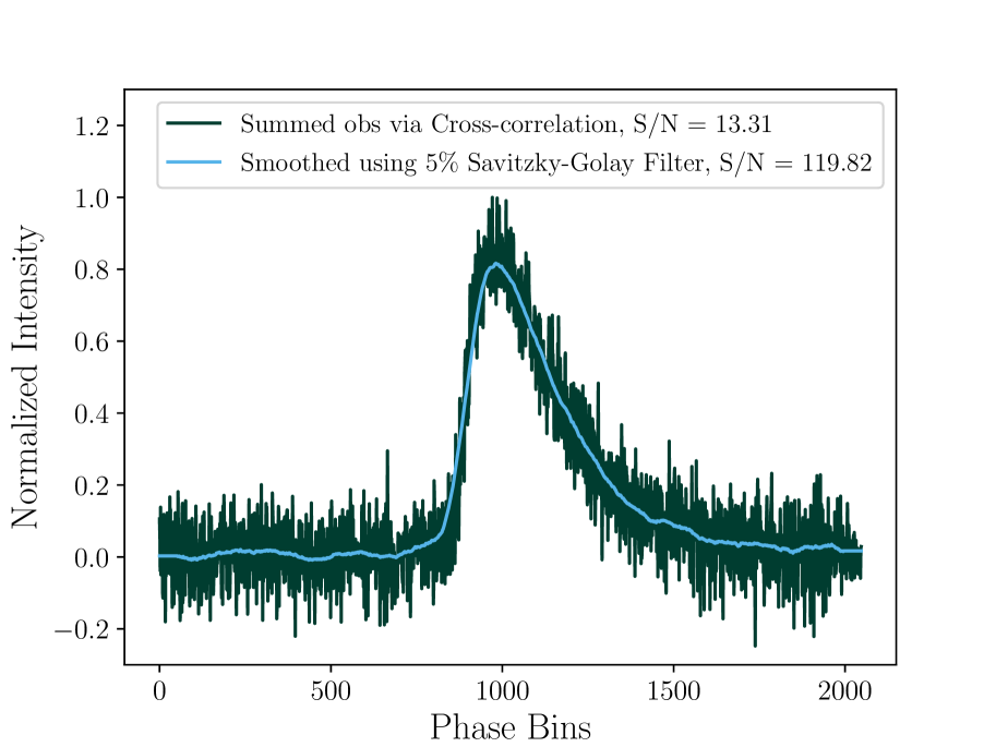
Figure 9: Summed and smoothed pulse profile for J1903+0327 at 1200 MHz from NANOGrav observations during 2014.

For our time series analysis, we used two different filtering techniques, both employing a Savitzky-Golay filter using a polynomial of order zero to fit the samples: using a filter window size necessary to achieve S/N of 70 and using a filter window of 5$\%$ of the observation length to achieve a higher S/N. We chose to create time series at two different levels of S/N to showcase the dependence of the algorithm’s performance on S/N. We iterated through test $\tau_{\rm d}$ values ranging from 100 to 500 bins for each run, with a step size of one bin. We see the results of these runs in Figures 10 and 11, where we converted our returned $\tau_{\rm d}$ values into units of microseconds.

Figure 10: Time series for PSR J1903+0327 from 2012 to 2017 using NANOGrav data. This time series is constructed using a Savitzky-Golay filter with a window filter size chosen to obtain a S/N of around 70.

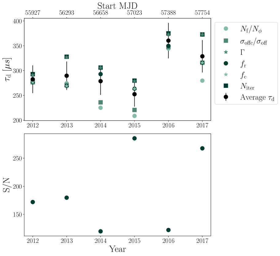
Figure 11: Time series for PSR J1903+0327 from 2012 to 2017 using NANOGrav data. This time series is constructed using a Savitzky-Golay filter with a window filter size of 5% of the length of the observation.

We see what is expected in the FOMs for these time series: greater precision and more visible points of change for the high S/N FOMs. Looking at Figures 12 and 13, we see examples of how higher S/N results in sharper points of change in the FOMs, thus making choosing the correct $\tau_{\rm d}$ a more precise process. While this is true for all FOMs prevented here, this difference can be seen most explicitly in the $\sigma_{\rm offc}$/$\sigma_{\rm off}$ FOM (panel 2), where there is a noticeable location where the slope begins increasing in our larger S/N FOMs, versus our lower S/N FOMs where there is a more gradual increase in the slope of the $\sigma_{\rm offc}$/$\sigma_{\rm off}$ FOM, making the correct $\tau_{\rm d}$ more difficult to pinpoint. This increased sharpness of the points of change of our FOMs translated into greater accuracy and better agreement across our FOMs, which can be seen reflected in the tighter clusters around the average returned $\tau_{\rm d}$ values in our time series.

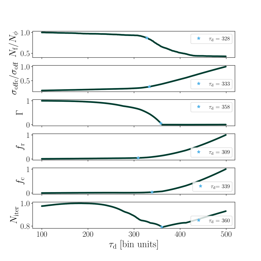
Figure 12: Normalized FOMs for PSR J1903+0327 at 1200 MHz from 2016 at S/N = 70. We see a tight grouping for the returned $\tau_{\rm d}$ values for each FOM, with a mean value of $\tau_{\rm d}=360.3~{}\mu$s and an error of 10% based on our simulation runs.

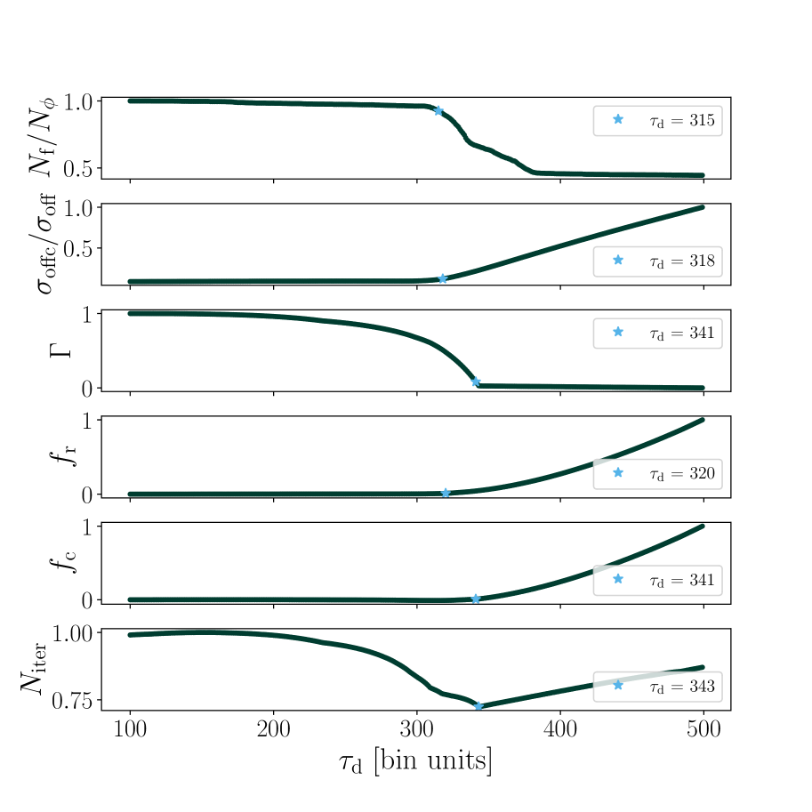
Figure 13: Normalized FOMs for PSR J1903+0327 at 1200 MHz from 2016 for high S/N values achieved by using a Savitzky-Golay filter with a window size of 5% of the length of the observation. We see an even tighter grouping for the returned $\tau_{\rm d}$ values for each FOM than compared to the lower S/N FOM, with a mean value of $\tau_{\rm d}=369.3~{}\mu$s and an error between 2% and 10% based on our simulation runs.

We also note some interesting results of this time series analysis, particularly the dip in 2015, followed by a drastic increase the following year. However, coupled with the unusual scattering indices measured in Geiger & Lam (2022), it is clear that an exponential PBF is not supported along this line of sight and a more complex model is necessary (Geiger et al. in prep). Nonetheless, we have shown via this analysis that not only does our CLEAN algorithm perform as expected on observational radio pulsar data given our et of assumptions, but also that employment of this algorithm holds potential for scientific insight into the ever-changing ISM.

5 Future work and Conclusions

Within this work, we discussed our motivations, introduced CLEAN deconvolution as presented in Bhat et al. (2003), discussed our results and products of our implementation of CLEAN, our parameterization work, and results on observational data of PSR J1903+0327. Through our parameterization work, we have concluded that our replicated CLEAN algorithm works as expected: the main factors that influence the recall of the algorithm are the S/N and $\tau_{\rm d}$ of the pulse profile, and higher values of S/N and $\tau_{\rm d}$ resulting in better recall. We have produced an algorithm that we can confidently deploy on larger sets of observational data. To that end, we have presented a brief analysis of PSR J1903+0327 at two S/N levels and discussed our findings, showing that our methods prove to be effective on observational data from radio pulsars and can thus provide insight into the time-dependence on pulse-broadening timescales for many pulsars after automatic deployment.

Moving forward, we aim to further develop our CLEAN algorithm into a broadly applicable tool, focusing on improving upon or removing the need for a number of simplifications used within this methods paper. We will also deploy our algorithm on the data set used in (Bhat et al., 2004), the followup to the original CLEAN method introductory paper, and on additional large-scale data sets (e.g., Stovall et al., 2015; Bilous et al., 2020). Using these data sets, we will use our CLEAN algorithm to provide measurements of $\tau_{\rm d}$ across multiple frequencies along many lines of sight. This will give us greater insight into both the composition of the ISM and the intrinsic emission of radio pulsars.

Within this work, we have extensively tested our algorithm’s performance on simulated pulses broadened using a thin-screen model of the ISM for our PBF. Future work will entail testing the effects of different pulse broadening functions, namely PBFs based on thick and uniform medium ISM models, on the performance of our algorithm. In addition, while our third derivative method for determining the intrinsic $\tau_{\rm d}$ from our FOMs works well given high levels of S/N and large $\tau_{\rm d}$ values, this may not hold for low $\tau_{\rm d}$ values and low levels of S/N as the FOMs are not as smooth. Therefore, we will work on improving our automation efforts via the implementation of machine learning, thus allowing our recall rates to better reflect the performance of the algorithm.

We have greatly simplified radio pulsar emission by assuming symmetric Gaussian intrinsic pulses. However, perfectly symmetric pulses are uncommon in radio pulsars (e.g., Bilous et al., 2016). Should the intrinsic pulse be non-symmetric, our $\Gamma$ FOM will either be completely ineffective or lead to incorrect values of $\tau_{\rm d}$ being chosen. Therefore, we must further probe the effects of non-symmetry on our FOM, and develop new FOMs that do not rely on assumed symmetry.

We have developed a Python-based CLEAN algorithm that behaves as expected, have parameterized the performance of this rebuilt algorithm on a variety of simulated test data sets, have developed a method to automate the process of choosing the correct $\tau_{\rm d}$ from our FOM, and have proved the efficacy of our algorithm on observational data. We have also defined areas of improvement for our algorithm, and look forward to continuing to develop a well-rounded method for probing the ISM using radio pulsars.

References

- Arzoumanian et al. (2021) Arzoumanian, Z., Baker, P. T., Blumer, H., et al. 2021, The Astrophysical Journal Letters, 923, L22, doi: 10.3847/2041-8213/ac401c
- Bhat et al. (2004) Bhat, N. D. R., Cordes, J. M., Camilo, F., Nice, D. J., & Lorimer, D. R. 2004, The Astrophysical Journal, 605, 759, doi: 10.1086/382680
- Bhat et al. (2003) Bhat, N. D. R., Cordes, J. M., & Chatterjee, S. 2003, 584, 782, doi: 10.1086/345775
- Bilous et al. (2016) Bilous, A. V., Kondratiev, V. I., Kramer, M., et al. 2016, A&A, 591, A134, doi: 10.1051/0004-6361/201527702
- Bilous et al. (2020) Bilous, A. V., Bondonneau, L., Kondratiev, V. I., et al. 2020, A&A, 635, A75, doi: 10.1051/0004-6361/201936627
- Cordes et al. (1986) Cordes, J. M., Pidwerbetsky, A., & Lovelace, R. V. E. 1986, ApJ, 310, 737, doi: 10.1086/164728
- Cordes & Rickett (1998) Cordes, J. M., & Rickett, B. J. 1998, ApJ, 507, 846, doi: 10.1086/306358
- Dolch et al. (2021) Dolch, T., Stinebring, D. R., Jones, G., et al. 2021, The Astrophysical Journal, 913, 98, doi: 10.3847/1538-4357/abf48b
- Geiger & Lam (2022) Geiger, A., & Lam, M. T. 2022, NANOGrav Memo Series No. 8, The Frequency-Dependent Scattering of Pulsar J1903+0327, Tech. rep., NANOGrav
- Högbom (1974) Högbom, J. A. 1974, A&AS, 15, 417
- Jones et al. (2013) Jones, G., Cordes, J., Demorest, P. B., et al. 2013, in 2013 US National Committee of URSI National Radio Science Meeting (USNC-URSI NRSM), 1–1, doi: 10.1109/USNC-URSI-NRSM.2013.6525028
- Lentati et al. (2017) Lentati, L., Kerr, M., Dai, S., et al. 2017, Monthly Notices of the Royal Astronomical Society, 468, 1474, doi: 10.1093/mnras/stx580
- Lorimer & Kramer (2004) Lorimer, D. R., & Kramer, M. 2004, Handbook of Pulsar Astronomy, Vol. 4
- Lorimer et al. (1997) Lorimer, D. R., D’Amico, N., Lyne, A. G., et al. 1997, in Joint European and National Astronomical Meeting, ed. J. D. Hadjidemetrioy & J. H. Seiradakis, 236
- Manchester et al. (2013) Manchester, R. N., Hobbs, G., Bailes, M., et al. 2013, PASA, 30, e017, doi: 10.1017/pasa.2012.017
- Shannon & Cordes (2017) Shannon, R. M., & Cordes, J. M. 2017, MNRAS, 464, 2075, doi: 10.1093/mnras/stw2449
- Stinebring (2013) Stinebring, D. 2013, Classical and Quantum Gravity, 30, 224006, doi: 10.1088/0264-9381/30/22/224006
- Stovall et al. (2015) Stovall, K., Ray, P. S., Blythe, J., et al. 2015, The Astrophysical Journal, 808, 156, doi: 10.1088/0004-637x/808/2/156
- Tsai et al. (2017) Tsai, Wei, J., Simonetti, J. H., & Kavic, M. 2017, PASP, 129, 024301, doi: 10.1088/1538-3873/129/972/024301
- Verbiest et al. (2016) Verbiest, J. P. W., Lentati, L., Hobbs, G., et al. 2016, MNRAS, 458, 1267, doi: 10.1093/mnras/stw347
- Williamson (1972) Williamson, I. P. 1972, Monthly Notices of the Royal Astronomical Society, Vol. 157, 55
- Young (2022) Young, O. 2022. https://scholarworks.rit.edu/theses/11294