UWThPh 2023-11
IPPP/23/19

Threshold factorization of the Drell-Yan
quark-gluon channel and two-loop soft function
at next-to-leading power

Alessandro Broggio,^a Sebastian Jaskiewicz,^b and Leonardo Vernazza^c

^a Faculty of Physics, University of Vienna,
Boltzmanngasse 5, A-1090 Vienna, Austria
^b Institute for Particle Physics Phenomenology, Durham University,
Durham DH1 3LE, United Kingdom
^c INFN, Sezione di Torino, Via P. Giuria 1, I-10125 Torino, Italy
and Dipartimento di Fisica Teorica, Università di Torino

We present a factorization theorem of the partonic Drell-Yan off-diagonal processes $g\bar{q}\,(qg)\to\gamma^{*}+X$ in the kinematic threshold regime $z=Q^{2}/\hat{s}\to 1$ at general subleading powers in the $(1-z)$ expansion. Focusing on the first order of the expansion (next-to-leading power accuracy with respect to the leading power $q\bar{q}$ channel), we validate the bare factorization formula up to $\mathcal{O}(\alpha^{2}_{s})$. This is achieved by carrying out an explicit calculation of the generalized soft function in $d$-dimensions using the reduction to master integrals and the differential equations method. The collinear function is a universal object which we compute from an operator matching equation at one-loop level. Next, we integrate the soft and collinear functions over the convolution variables and remove the remaining initial state collinear singularities through PDF renormalization. The resulting expression agrees with the known cross section in the literature.

1 Introduction

It is well documented that the perturbative expansion of QCD fails near the kinematic threshold, as the phase space for real emission is restricted to contain only low-energy (soft) radiation. Considering the Drell-Yan (DY) process $A(p_{A})+B(p_{B})\to\gamma^{*}(Q)[\to\ell\bar{\ell}\,]+X$, with $X$ being the unobserved QCD final state, the threshold regime of the partonic cross section is characterised by the limit $z\equiv Q^{2}/\hat{s}\to 1$, where $Q^{2}$ represents the invariant mass of the final state lepton pair and $\hat{s}$ the partonic centre-of-mass energy squared. In this region, physical observables are expressed as a power expansion in $(1-z)\to 0$ and feature large logarithmic corrections in this variable. Reliable results can only be obtained by resumming these logarithms to all orders in perturbation theory. This was first achieved for the leading-power (LP) contribution more than thirty years ago using diagrammatic techniques in [1, 2] and later using soft-collinear effective theory (SCET) methods in [3, 4, 5].

Nowadays the resummation of LP threshold logarithms is understood in DY up to next-to-next-to-next-to-leading logarithmic (N³LL) accuracy [6, 7, 8, 9]. However, comparatively less is known about terms which are suppressed by a power of $(1-z)$, the so-called next-to-leading power (NLP) logarithms, despite the fact that studies of amplitudes with next-to-soft emissions have quite a long history [10, 11, 12]. Focusing on the diagonal ($q\bar{q}$) channel of the Drell-Yan process, calculations of partonic cross sections at NLP up to next-to-next-to-leading order (NNLO) in the strong coupling expansion, and partly beyond, have been carried out using the expansion-by-regions method [13, 14] and diagrammatic factorization techniques [15, 16, 17, 18, 19]. Investigations of the NLP terms for the DY process within the effective field theory (EFT) framework were initiated in [20] and [21]. In the former, the NLP logarithms were resummed to leading logarithmic (LL) accuracy, and in the latter, the complete subleading power factorization theorem was derived. In the present work, we complete these investigations by deriving and validating up to NNLO the NLP factorization theorem for the off-diagonal $g\bar{q}\,(qg)$ channel of the DY production process at threshold, which constitutes the last missing piece up to NLP accuracy.

The development of this framework is timely as plenty of attention has recently been given to NLP studies of the analogous off-diagonal channels in deep-inelastic scattering (DIS) at large Bjorken-$x$ and “gluon thrust” in hadronic $e^{+}e^{-}$ annihilation, their corresponding diagonal channels, and Higgs production in gluon fusion at threshold [19, 22, 20, 23, 24, 25, 26, 21, 27, 28, 29, 30, 31, 32]. Progress beyond LP has also been achieved for variables such as N-jettiness [33, 34, 35, 36, 37, 38] and the $q_{T}$ of the lepton pair or the Higgs boson [39, 40, 41]. However, the extension of the standard LP factorization theorems to NLP has not proved straightforward. The main stumbling block being the ubiquitous appearance of endpoint divergences in the convolution integrals that connect the hard, (anti-) collinear and soft functions in NLP factorization theorems [21]. This conceptual issue has been investigated in a number of contexts: for instance, conjecture regarding the form of the leading double logarithms related to soft quark emission has been presented in [26], and refactorization ideas were developed for DIS [29] and for Higgs decay to two photons (and gluons) through bottom-quark loops [42, 43, 44, 45]. Combination of standard SCET factorization and endpoint factorization was put forward in [32] to arrive at a factorization formula for the “gluon thrust” valid in $d=4$, such that standard systematically improvable Renormalization Group (RG) methods can be applied to perform the resummation of large logarithms. Endpoint divergences have also recently been explored in QED [46] and $B$ physics [47, 48, 49].

Concerning the study of the all-order resummation for the $g\bar{q}$ channel of DY, results at LL accuracy have recently been obtained using diagrammatic techniques in[31] and $d$-dimensional consistency relations in[50]. In general, the development of a resummation framework at higher orders will require a genuine prescription for the treatment of the endpoint convolution divergences in the presence of hadronic initial states. In this respect, it is crucial to derive a consistent factorization theorem valid in $d=4$. As a first step toward this goal, however, one needs to develop a consistent factorization theorem at the level of the bare cross section, and calculate all of the contributing functions to the relevant perturbative order in dimensional regularization. While this task has been completed for the DY $q\bar{q}$ channel in [21, 51], the $g\bar{q}$ channel of DY has not been systematically address yet. The purpose of this paper is to fill this gap: in particular, starting from time-ordered power suppressed operators in SCET, we derive the factorization of the partonic cross section in terms of short-distance coefficients times the convolution of collinear and soft matrix elements, valid at any subleading power. We then focus on the NLP contribution, and evaluate the collinear and soft functions appearing in the factorization theorem respectively at $\mathcal{O}(\alpha_{s})$ and $\mathcal{O}(\alpha^{2}_{s})$, which is the required accuracy to reproduce the known inclusive DY cross section result at NNLO. This provides a strong sanity check of our framework and allows us to reach the same accuracy as for the diagonal $q\bar{q}$ channel in [21, 51].

The collinear function has a purely virtual origin and we evaluate it at one-loop order. Its appearance is the consequence of the insertion of the power suppressed interaction which couples a soft quark with collinear gluons and a collinear quark. This function is practically equivalent (with just some minor differences in its definition) to the radiative collinear function computed to $\mathcal{O}(\alpha^{2}_{s})$ in [52]. The calculation of the collinear function which appears in the factorization formula for the $g\bar{q}$ channel turns out to be much simpler in comparison to the evaluation of the collinear functions which appear in [21] since the derivative terms acting on the momentum conserving delta function are not present in this case. The soft function depends on the total energy of the soft emissions as well as two additional convolution variables. We evaluate the soft contributions at NNLO accuracy in exact $d$-dimensions by employing the reduction to master integrals and the differential equations methods that were also employed in [51]. Other soft functions which appear in the $h\to\gamma\gamma$ decay NLP factorization formula were computed in [53, 54] at $\mathcal{O}(\alpha_{s})$.

Working with $d$-dimensional expressions allows us to carry out the convolution integrals at fixed-order accuracy. This is the first step needed for the application of the refactorization ideas developed in [32, 44]. We also study asymptotic limits of the obtained functions which is useful for any such program. However, additional insights concerning the operatorial structure of the incoming hadronic states are required to carry out this program, which we leave to a future investigation.

The paper is organised as follows: in section 2 we derive the general subleading power factorization formula for the partonic off-diagonal channels of the DY process and we specialize it to NLP. Then, in sections 3 and 4 we calculate the required NLP collinear and generalized soft functions up to $\mathcal{O}(\alpha_{s})$ and $\mathcal{O}(\alpha_{s}^{2})$, respectively. As a last step in section 4, we consider asymptotic limits of the soft function. The obtained accuracy of the soft and collinear functions enables the validation of the factorization formula derived in section 2 to NNLO, which is carried out in section 5. We summarize and discuss possible future developments in section 6.

2 Factorization near threshold

We consider the Drell-Yan invariant mass distribution

$$\frac{d\sigma_{\rm DY}}{dQ^{2}}=\frac{4\pi\alpha_{\rm em}^{2}}{3N_{c}Q^{4}}\sum_{a,b}\int_{\tau}^{1}dz\int dx_{a}dx_{b}\,\delta\bigg{(}z-\frac{\tau}{x_{a}x_{b}}\bigg{)}f_{a/A}(x_{a})f_{b/B}(x_{b})\,\hat{\sigma}_{ab}(z)+\mathcal{O}\left(\frac{\Lambda}{Q}\right),$$ (2.1)

where $f_{a/A}(x_{a})$ and $f_{b/B}(x_{b})$ are the usual parton distribution functions (PDFs) of partons $a$, $b$, with momentum fractions $x_{a}$, $x_{b}$; $\hat{\sigma}_{ab}(z)$ represents the partonic cross section for the process $a(p_{a})b(p_{b})\to\gamma^{*}(q)[\to\ell\bar{\ell}\,]+X$; $\tau=Q^{2}/s$ and $z=Q^{2}/\hat{s}$ are respectively the hadronic and partonic threshold variables, with $s=(p_{A}+p_{B})^{2}$ and $\hat{s}=(p_{a}+p_{b})^{2}=x_{a}x_{b}\,s$ the hadronic and partonic centre of mass energy; $Q^{2}\equiv q^{2}$ is the invariant mass of the final state photon; last, $\Lambda$ is the confinement scale of QCD. In the present analysis, we do not consider power corrections in $\Lambda/Q$.

Near threshold the partonic cross section has the following power expansion

$$\hat{\sigma}_{ab}(z)=\hat{\sigma}^{\,{\rm{LP}}}_{ab}(z)\,+{\hat{\sigma}^{\,{\rm{NLP}}}_{ab}(z)}+\mathcal{O}(\lambda^{2}),$$ (2.2)

where the power-counting parameter is defined as $\lambda=\sqrt{1-z}\ll 1$; the leading power term in the equation above is ${\cal O}(\lambda^{-2})$ and the next-to-leading power term is ${\cal O}(\lambda^{0})$. Only the diagonal production channel $ab=q\bar{q}$ contributes at LP. At NLP more channels open up: in addition to the NLP correction to the $q\bar{q}$ channel, which has been studied at length in [21, 51], there are also contributions from the gluon-antiquark $g\bar{q}$ and the quark-gluon $qg$ channels, which are the topic of the present work. In this section we derive their factorization structure near threshold, valid at general subleading powers. Given that the two channels $g\bar{q}$ and $qg$ give identical contributions, in what follows we focus for simplicity on the gluon-antiquark $g\bar{q}$ channel.

We derive the factorization theorem for the bare cross section in $d=4-2\epsilon$ dimensions: in this case, dimensional regularization regulates the endpoint divergences arising in convolution integrals, hence calculations at fixed orders are well defined. In order to facilitate comparison with literature, we will consider an equivalent form of Eq. (2.1), given by

$$\frac{d\sigma_{\rm DY}}{dQ^{2}}=\sigma_{0}\sum_{a,b}\int_{\tau}^{1}\,\frac{dz}{z}\,{\cal L}_{ab}\bigg{(}\frac{\tau}{z}\bigg{)}\,\Delta_{ab}(z)+\mathcal{O}\left(\frac{\Lambda}{Q}\right),\qquad\sigma_{0}=\frac{4\pi\alpha_{\rm em}^{2}}{3N_{c}Q^{2}s},$$ (2.3)

where the parton luminosity function ${\cal L}_{ab}(y)$ is defined as

$${\cal L}_{ab}(y)=\int_{y}^{1}\frac{dx}{x}\,f_{a/A}(x)\,f_{b/B}\bigg{(}\frac{y}{x}\bigg{)},$$ (2.4)

and $\Delta_{ab}(z)$ is related to the partonic cross section $\hat{\sigma}_{ab}(z)$ in Eq. (2.1) by

$$\Delta_{ab}(z)=\frac{1}{(1-\epsilon)}\frac{\hat{\sigma}_{ab}(z)}{z}\,.$$ (2.5)

In order to obtain the factorization theorem for $\Delta_{g\bar{q}}(z)$ let us start from the standard expression for the hadronic $d$-dimensional differential cross section. After integration over the phase-space for the final state leptons one has

$$d\sigma=\frac{4\pi\alpha_{{\rm{em}}}^{2}}{3s\,q^{2}}\frac{d^{d}q}{(2\pi)^{d}}\,\big{(}-g^{\mu\rho}\,W_{\mu\rho}\big{)}\,,$$ (2.6)

where $W_{\mu\rho}$ is the hadronic tensor

$$g^{\mu\rho}W_{\mu\rho} = \int d^{d}x\,e^{-iq\cdot x}\,\langle A(p_{A})B(p_{B})|J^{\dagger\,\rho}(x)J_{\rho}(0)|A(p_{A})B(p_{B})\rangle$$ (2.7)

$$= \sum_{X}\,(2\pi)^{d}\delta^{(d)}\left(p_{A}+p_{B}-q-p_{X_{s}}-p_{X_{c}^{\rm PDF}}-p_{X_{\bar{c}}^{\rm PDF}}\right)$$

$$\times\,\langle A(p_{A})B(p_{B})|J^{\dagger}_{\rho}(0)|X\rangle\langle X|J^{\rho}(0)|A(p_{A})B(p_{B})\rangle\,,$$

and in turn $J^{\rho}=\sum_{q}e_{q}\bar{\psi}_{q}\gamma^{\rho}\psi_{q}$ represents the electromagnetic quark current. In Eq. (2.7), $p_{X_{s}}+p_{X_{c}^{\rm PDF}}+p_{X_{\bar{c}}^{\rm PDF}}=p_{X}$ is the total momentum of the final state radiation $X$. In order to not obscure the derivation of the factorization theorem, in what follows we work with a single quark flavour and set the electromagnetic charge $e_{q}=1$.

The partonic kinematic threshold corresponds to the case where almost all of the energy in the interaction between the two incoming partons is carried away by the intermediate off-shell boson, $\gamma^{*}$. The relevant modes consist thus of PDF-collinear and PDF-anticollinear modes, threshold-collinear and threshold-anticollinear modes, and soft modes. Momenta are decomposed along two light-like directions $n_{\pm}^{\mu}$, defined by $n_{-}^{\mu}=2p_{A}^{\mu}/\sqrt{s}$, $n_{+}^{\mu}=2p_{B}^{\mu}/\sqrt{s}$, such that a generic momentum $l^{\mu}$ has decomposition $l^{\mu}=n_{+}l\,n_{-}^{\mu}/2+n_{-}l\,n_{+}^{\mu}/2+l^{\mu}_{\perp}$. The scaling of a given momentum $l^{\mu}$ is thus indicated by the scaling of the components $(n_{+}l,l_{\perp},n_{-}l)$. The PDF-collinear and anticollinear modes scale respectively as $p_{X_{c}^{\rm PDF}}^{\mu}\sim(Q,\Lambda,\Lambda^{2}/Q)$ and $p_{X_{\bar{c}}^{\rm PDF}}^{\mu}\sim(\Lambda^{2}/Q,\Lambda,Q)$, where $\Lambda\ll Q\lambda=Q(1-z)^{1/2}$ represents the confinement scale of QCD, while threshold collinear, anticollinear, and soft modes scales respectively as $p_{c}~{}\sim~{}Q(1,\lambda,\lambda^{2})$, $p_{\bar{c}}~{}\sim~{}Q(\lambda^{2},\lambda,1)$ and $p_{s}~{}\sim~{}Q(\lambda^{2},\lambda^{2},\lambda^{2})$. We work in position-space SCET [55, 56] and describe each mode by its own set of fields. We have therefore PDF- and threshold-collinear quarks and gluons, and soft quarks and gluons. These fields are expressed in terms of gauge-invariant building blocks, after the soft-collinear decoupling transformation has been applied. For instance, we express collinear fields modes in terms of the gauge-invariant building blocks

$$\chi^{(0)}_{c}(z) = Y_{+}^{\dagger}(z_{-})\chi_{c}(z),\qquad\mathcal{A}^{(0)\mu}_{c}(z)=Y_{+}^{\dagger}(z_{-})\mathcal{A}^{\mu}_{c}(z)Y_{+}(z_{-}),$$ (2.8)

where $\chi_{c}=W_{c}^{\dagger}\xi_{c}$ and $\mathcal{A}_{c}^{\mu}=W_{c}^{\dagger}\left[iD_{c}^{\mu}\,W_{c}\right]$ represent the original non-decoupled collinear fields. In turn, the covariant derivative is defined as $iD_{c}^{\mu}=i\partial^{\mu}+g_{s}A^{\mu}_{c}$. In what follows we will always work with decoupled fields, and drop the index $(0)$. In Eq. (2.8) the soft Wilson lines are defined as

$$Y_{\pm}\left(x\right) = \mathbf{P}\exp\left[ig_{s}\int_{-\infty}^{0}ds\,n_{\mp}A_{s}\left(x+sn_{\mp}\right)\right],$$ (2.9)

while the collinear Wilson lines reads

$$W_{c}\left(x\right) = \mathbf{P}\exp\left[ig_{s}\int_{-\infty}^{0}ds\,n_{+}A_{c}\left(x+sn_{+}\right)\right].$$ (2.10)

In both of the above equations $\mathbf{P}$ is the path ordering operator. Notice also that in eq. (2.8) the soft Wilson lines are evaluated at $z_{-}^{\mu}\equiv(n_{+}z)n_{-}^{\mu}/2$, in accordance with the fact that soft fields are multipole expanded when multiplying collinear fields [56]. Concerning soft fields, we write them in terms of the gauge invariant building blocks

$${q}^{\pm}=Y_{\pm}^{\dagger}\,q_{s}\,.\qquad\mathcal{B}_{\pm}^{\mu}=Y_{\pm}^{\dagger}\left[i\,D^{\mu}_{s}\,Y_{\pm}\right]\,,$$ (2.11)

where the soft covariant derivative is $iD_{s}^{\mu}=i\partial^{\mu}+g_{s}A^{\mu}_{s}$. The power-suppressed soft-collinear Lagrangian $\mathcal{L}^{(i)}=\mathcal{L}^{(i)}_{\xi}+\mathcal{L}^{(i)}_{\xi q}+\mathcal{L}^{(i)}_{\rm YM}$ is then expressed in terms of these fields, as listed in appendix A of [21]. We refer to [55, 56] for a thorough derivation of the SCET Lagrangian and SCET fields definition.

Given that the final state is forced to only contain soft radiation, the hard matching to SCET fields can be performed at amplitude level, since there are no contributions to the hadronic tensor where the currents at positions $0$ and $x$ are connected by hard partons. For the process $g\bar{q}\,\rightarrow\,\gamma^{*}+X$ to take place in the $z\to 1$ limit, the incoming $c$-PDF gluon must be converted to a threshold collinear quark through the emission of a soft antiquark. The threshold-collinear quark retains almost all of the momentum of the incoming $c$-PDF gluon. The soft-quark interaction with collinear fields is inherently a subleading power effect. This can be deduced from the fact that soft quarks at leading power only appear in the soft term, $\bar{q}_{s}i\not{D}_{s}q_{s}$, in the SCET Lagrangian; the soft quarks first appear in soft-collinear interaction terms at $\mathcal{O}(\lambda)$ in $\mathcal{L}^{(1)}_{\xi q}$,

$$\mathcal{L}^{(1)}_{\xi q}=\bar{q}^{\,+}\ThisStyle{\ensurestackMath{{\stackinset{r}{}{c}{}{\SavedStyle/}{\SavedStyle\mathcal{A}}}}}_{c\perp}\chi_{c}+{\rm h.c.}.$$ (2.12)

Therefore, unlike in the case of the $q\bar{q}$-channel discussed in [21], the contribution to the Drell-Yan cross-section from the $g\bar{q}$-channel begins at NLP (i.e., at ${\cal O}(\lambda^{2})$), through a time-ordered product insertion of $\mathcal{L}^{(1)}_{\xi q}$ into the amplitude and its complex conjugate, as represented in Fig. 1.

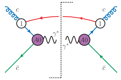
Figure 1: Schematic representation of the lowest-power contribution to the gluon-antiquark channel in Drell-Yan. It involves the conversion of a (PDF) collinear gluon into a (threshold) collinear quark by emission of a soft anti-quark. The emission proceeds first at NLP by means of a time-ordered product, involving the leading power SCET current $J^{A0}$ times the insertions of the power suppressed Lagrangian ${\cal L}_{\xi q}^{(1)}$, indicated by the index “1” in the picture. The matching of threshold modes onto PDF modes is trivial for the anti-collinear sector, as there is no power suppression on this leg [21].

2.1 Factorization at general subleading powers

The formal factorization formula for the $g\bar{q}$-channel at general subleading can be obtained following closely the derivation for the $q\bar{q}$-channel given in [21], therefore we provide here a rather concise discussion and draw attention to the differences between the two cases. Our discussion below follows the derivation given in [57]. In general, one needs to take into account the contribution of time-ordered products involving the (multiple) insertions of $\mathcal{L}^{(i)}=\mathcal{L}^{(i)}_{\xi}+\mathcal{L}^{(i)}_{\xi q}+\mathcal{L}^{(i)}_{\rm YM}$ Lagrangian terms and operators arising from the expansion of the Drell-Yan current, with the constraint that the time-ordered products must involve a collinear gluon and at least one soft quark emission. Omitting the index structure for clarity, the general, all power, hard matching of the vector current is given by

$$\bar{\psi}\gamma_{\rho}\psi(0)=\sum_{m_{1},{m_{2}}}\,\int\{dt_{k}\}\,\{d\bar{t}_{\bar{k}}\}\,\widetilde{C}^{\,m_{1},m_{2}}\left(\,\{t_{k}\},\,\{\bar{t}_{\bar{k}}\}\right)\,J_{s}(0)\,J_{\rho}^{\,m_{1},m_{2}}\left(\,\{t_{k}\},\,\{\bar{t}_{\bar{k}}\}\right)\,,\quad$$ (2.13)

where the symbols $\{dt_{k}\}$, $\{t_{k}\}$ (and the barred ones for the anticollinear direction) indicate sets of convolution variables associated to the number of fields in each collinear direction. The indices $m_{1}$ and $m_{2}$ label the basis of SCET operators (and their corresponding short-distance matching coefficients $\widetilde{C}^{\,m_{1}m_{2}}$), following the formalism and notation developed in [58, 59, 60]. The function $J_{s}$ involves only soft fields and starts at $\mathcal{O}(\lambda^{3})$ [58]. Given that the DY process involves a collinear and an anticollinear direction, the currents $J_{\rho}^{\,m_{1},m_{2}}$ explicitly read

$$J_{\rho}^{\,m_{1},m_{2}}\left(\,\{t_{k}\},\,\{\bar{t}_{\bar{k}}\}\right)=J^{\,m_{1}}_{\bar{c}}\left(\{\bar{t}_{\bar{k}}\}\right)\,\Gamma_{\rho}^{m_{1},m_{2}}\,J^{\,m_{2}}_{c}\left(\{t_{k}\}\right)\,,$$ (2.14)

where for instance the terms $J^{\,m_{2}}_{c}\left(\,\{t_{k}\}\right)$ are constructed using collinear-gauge-invariant collinear building blocks given in Eq. (2.8). In this general construction, the indices $m_{1}$, $m_{2}$ consist of letters $A$, $B$, $C$ etc., labelling the number of fields in a particular collinear direction, and numbers 0, 1, 2 etc., denoting the overall power of $\lambda$ of the current with respect to the LP, which is labelled $0$. The function $\Gamma_{\rho}^{m_{1},m_{2}}$ in Eq. (2.14) gives the appropriate spinor and Lorentz structure of the operator. For instance, the structure of the LP operator reads $\Gamma^{\,A0,A0}_{\rho}=\gamma_{\perp\rho}\,$; at $\mathcal{O}(\lambda)$ one has $\Gamma^{\,A0,A1}_{\rho}=n_{+\rho}$, etc.

Hard modes are integrated out in the matching between QCD and SCET, and appear as short-distance coefficients $\widetilde{C}^{\,m_{1},m_{2}}$ in Eq. (2.13). In the next step, one integrates out threshold-collinear and anticollinear modes. As discussed in [20, 21], this gives rise to a matching equation, which involves on the left-hand-side the SCET Lagrangian with threshold-collinear and soft fields, and on the right-hand side PDF-collinear and soft fields, times a short-distance coefficient, defined as “collinear function”, which arises as a consequence of integrating out threshold-collinear modes. The collinear function is the analogue of the “radiative jet” discussed in [12, 18, 19], and we refer to section 2 of [21] for a detailed discussion. The specific form of the matching equation is dictated by gauge invariance, momentum and Fermion number conservation. For the $g\bar{q}$ channel, the general collinear matching equation reads

$$i^{\,m}\int\{d^{d}z_{j}\}\,T\left[\,\{\psi_{c}(t_{k}n_{+})\}\times\left\{\mathcal{L}^{(l)}(z_{j})\right\}\right]$$

$$\hskip 28.45274pt=2\pi\sum_{i}\int du\int\{dz_{j-}\}\,\tilde{G}_{i}\left(\{t_{k}\},u;\{z_{j-}\}\right)\,\frac{1}{g_{s}}{\cal A}^{\text{\scriptsize PDF}}_{c}(un_{+})\,\mathfrak{s}_{i}(\{z_{j-}\})\,,$$ (2.15)

where $\{d^{d}z_{j}\}=\prod^{m}_{j=0}\,d^{d}z_{j}$ and $\{dz_{j-}\}=\prod^{m}_{j=0}\frac{dn_{+}z_{j}}{2}$. $\{z_{j-}\}$ denotes the set of $m$ positions at which the soft building block insertions are located, and $T$ represents the time-ordering operator. On the left-hand side, $\left\{\mathcal{L}^{(l)}(z_{j})\right\}$ is a set of $m$ $\mathcal{O}(\lambda^{l})$-suppressed Lagrangian insertions and $\{\psi_{c}(t_{k}n_{+})\}$ denotes a set of $n$ collinear fields, $\psi_{c}=\chi_{c}$ or $\mathcal{A}^{\mu}_{c\perp}$, each dependent on one variable from the $n$-sized set $\{t_{k}\}$, originating from the collinear part of the Drell-Yan current operators. On the right-hand side, the function $\tilde{G}_{i}$ represents the NLP collinear function resulting from the matching of threshold collinear fields onto the initial state PDF-collinear gluon ${\cal A}_{c}^{\text{\scriptsize PDF}}$ and is analogous to the NLP collinear function $\tilde{J}_{i}$ in [20, 21], representing the matching onto an initial state PDF-collinear quark, which appears in the factorization of the $q\bar{q}$ channel. Last, as in case of the $q\bar{q}$ channel, the soft operator $\mathfrak{s}_{i}(\{z_{j-}\})$ represents a series of soft structures, containing the soft fields originating from the power-suppressed soft-collinear interaction. In case of the $g\bar{q}$ channel $\mathfrak{s}_{i}(\{z_{j-}\})$ must contain at least one soft quark, i.e.

$$\mathfrak{s}_{i}(\{z_{j-}\})\hskip 2.84544pt \in \hskip 4.26773pt\bigg{\{}\frac{g_{s}}{in_{-}\partial_{z}}q^{+}(z_{-}),\,\ldots\,\bigg{\}}\,,$$ (2.16)

where the index $i$ labels the soft structures, and the ellipsis refers to additional structures appearing beyond NLP. Note that, for consistency with the $q\bar{q}$ channel, we normalise the collinear function such that at tree level it contributes to ${\cal O}(g_{s}^{0})$, and we absorb a factor of $g_{s}$ into the soft structures, as can be seen explicitly in Eq. (2.16). Notice also that the collinear gauge invariant building block itself contains a factor of $g_{s}$, which is compensated by the explicit factor of $g_{s}^{-1}$ in Eq. (2.1). The matching for the anticollinear leg, with an incoming antiquark, is analogous to Eq. (2.1), and involves the anticollinear function $\bar{\tilde{J}}_{\,\bar{i}}$, as for the $q\bar{q}$ case, and the soft structures given in Eq. (3.45) of [21]. After the second matching onto collinear and anticollinear PDF modes has been performed, the derivation of the factorization theorem follows very closely that of the $q\bar{q}$ channel. Taking into account the factorization of the state $|X\rangle=|X_{c}\rangle\otimes|X_{\bar{c}}\rangle\otimes|X_{s}\rangle$, the $g\bar{q}$ matrix element reads

$$\langle X|\bar{\psi}\gamma_{\rho}\psi(0)|A(p_{A})B(p_{B})\rangle = \sum_{m_{1},m_{2}}\,\sum_{i,\bar{i}}\,\int\,\{dt_{k}\}\,\{d\bar{t}_{\bar{k}}\}\,\widetilde{C}^{\,m_{1},m_{2}}\left(\,\{t_{k}\},\,\{\bar{t}_{\bar{k}}\}\right)$$ (2.17)

$$\times\,2\pi\int d\bar{u}\int\{d\bar{z}_{\,\bar{j}+}\}\,\bar{\tilde{J}}_{\,\bar{i}}^{\,m_{1}}\left(\,\{\bar{t}_{\bar{k}}\},\bar{u};\{\bar{z}_{\,\bar{j}+}\}\right)\,\langle X^{{\rm PDF}}_{\bar{c}}|\bar{\chi}^{{\rm PDF}}_{\bar{c}}(\bar{u}n_{-})|B(p_{B})\rangle$$

$$\times\,2\pi\int du\int\{dz_{j-}\}\,\tilde{G}^{\,m_{2}}_{i}\left(\,\{t_{k}\},u;\{z_{j-}\}\right)\,\langle X^{{\rm PDF}}_{{c}}|\frac{1}{g_{s}}\mathcal{A}^{{\rm PDF}}_{c\perp}(un_{+})|A(p_{A})\rangle$$

$$\times\,\Gamma^{m_{1},m_{2}}_{\rho}\,\langle X_{s}|\,T\left(\bar{\mathfrak{s}}_{\,\bar{i}}\,(\,\{\bar{z}_{\,\bar{j}+}\})\,\big{[}Y_{-}^{\dagger}\,J_{s}\,Y_{+}\big{]}(0)\,\mathfrak{s}_{i}\,(\{z_{j-}\})\right)|0\rangle\,,$$

where explicit Dirac, Lorentz, and color indices are suppressed. The index $k$ $(\bar{k})$ counts the number of collinear (anticollinear) building block fields in a given current, and we sum over all of the possible currents. The index $j$ $(\,\bar{j}\,)$ counts the number of insertions of the subleading power Lagrangians into each collinear (anticollinear) sector, and again we sum over all of the occurrences.

In order to take the square of the matrix element in Eq. (2.17) it proves useful to write it in terms of the momentum-space representation of the various functions, which are obtained by means of Fourier transformation. For the short-distance coefficients $\widetilde{C}^{\,m_{1},\,m_{2}}$ one has

$$\widetilde{C}\left(\{t_{k}\},\{\bar{t}_{\bar{k}}\}\,\right)=\int\left\{\frac{dn_{+}p_{k}}{2\pi}\right\}\left\{\frac{dn_{-}\bar{p}_{\,\bar{k}}}{2\pi}\right\}\,e^{i\,(n_{+}p_{k})\,t_{k}}e^{i\,(n_{-}\bar{p}_{\,\bar{k}})\,\bar{t}_{\bar{k}}}\,C(\{n_{+}p_{k}\},\{n_{-}\bar{p}_{\,\bar{k}}\}),$$ (2.18)

then we need to introduce the momentum-space representation of the PDF-collinear and anticollinear fields. For instance, for the $c$-PDF gluon field we use

$${\mathcal{A}^{\rm{PDF}}_{c\perp}(un_{+})=\int\frac{dn_{+}p_{a}}{2\pi}e^{-i(n_{+}p_{a})u}\hat{\mathcal{A}}^{\rm{PDF}}_{c\perp}(n_{+}p_{a})},$$ (2.19)

with analogous definition for the $\bar{c}$-PDF antiquark field. Furthermore, the Fourier transform of the collinear function is given as

$$\int\{dt_{k}\}\int du\,\tilde{G}^{m_{2}}_{\,{i}}\left(\,\{t_{k}\},\,u;\,\{\,z_{j-}\}\,\right)\,e^{i(n_{+}p_{k})\,t_{k}}e^{-i(n_{+}p_{a})\,u}$$

$$=\int\,\left\{\frac{d\omega_{j}}{2\pi}\right\}\,\,e^{-i\omega_{j}z_{j-}}\,{G}^{m_{2}}_{\,{i}}\left(\,\{n_{+}p_{k}\},n_{+}p_{a};\,\{\omega_{j}\}\right)\,,$$ (2.20)

with an analogous definition for the anticollinear function. Here the set $\{\omega_{j}\}$ denotes the variables with a soft scaling that are conjugate to $\{\,z_{j-}\}$ and in the exponents Einstein’s summation convention is used. Also, $\left\{\frac{d\omega_{j}}{2\pi}\right\}=\frac{d\omega_{1}}{2\pi}\times...\times\frac{d\omega_{m}}{2\pi}$.

Making use of these definitions, Eq. (2.17) becomes

$$\langle X|\bar{\psi}\gamma_{\rho}\psi(0)|A(p_{A})B(p_{B})\rangle = \sum_{m_{1},m_{2}}\,\sum_{i,\bar{i}}\,\int\left\{\frac{dn_{+}p_{k}}{2\pi}\right\}\,\left\{\frac{dn_{-}\bar{p}_{\,\bar{k}}}{2\pi}\right\}$$ (2.21)

$$\times\int\,d(n_{+}p_{a})\,\,d(n_{-}p_{b})\,C^{\,m_{1},m_{2}}(\{n_{+}p_{k}\},\,\{n_{-}\bar{p}_{\bar{k}}\})$$

$$\times\,\int\left\{\frac{d\bar{\omega}_{\,\bar{j}}}{2\pi}\right\}\,\bar{J}^{\,m_{1}}_{\,\bar{i}}\left(\,\{n_{-}\bar{p}_{\bar{k}}\},-n_{-}p_{b};\,\{\bar{\omega}_{\,\bar{j}}\}\right)\,\,\langle X^{{\rm PDF}}_{\bar{c}}|\hat{\bar{\chi}}^{{\rm PDF}}_{\bar{c}}(n_{-}p_{b})|B(p_{B})\rangle$$

$$\times\,\int\left\{\frac{d\omega_{j}}{2\pi}\right\}\,{G}^{\,m_{2}}_{\,{i}}\left(\,\{n_{+}p_{k}\},n_{+}p_{a};\,\{\omega_{j}\}\right)\,\langle X^{{\rm PDF}}_{{c}}|\frac{1}{g_{s}}\hat{\mathcal{A}}^{{\rm PDF}}_{c\perp}(n_{+}p_{a})|A(p_{A})\rangle$$

$$\times\,\Gamma^{m_{1},m_{2}}_{\rho}\int\{d\bar{z}_{\,\bar{j}+}\,\}\int\{dz_{j-}\}\,e^{-i\bar{\omega}_{\,\bar{j}}\,\bar{z}_{\,\bar{j}+}}\,\,e^{-i\omega_{j}\,z_{j-}}$$

$$\times\,\langle X_{s}|\,T\left(\bar{\mathfrak{s}}_{\,\,\bar{i}}\,(\{\bar{z}_{\,\bar{j}+}\})\left[Y_{-}^{\dagger}\,J_{s}\,Y_{+}\right](0)\,\mathfrak{s}_{i}(\{z_{j-}\})\right)|0\rangle\,.$$

The matrix element can be written in a more compact form by introducing the following amplitude level coefficient functions

$$\mathcal{D}^{m_{1},m_{2}\,\rho}_{\,{i}\,\bar{i}}(n_{+}p_{a},-n_{-}{p}_{b};\,\{\omega_{j}\},\,\{\bar{\omega}_{\bar{j}}\}) = (2\pi)^{2}\int\left\{\frac{dn_{+}p_{k}}{2\pi}\right\}\,\left\{\frac{d(n_{-}\bar{p}_{\bar{k}})}{2\pi}\right\}$$ (2.22)

$$\times\,C^{\,m_{1},m_{2}}(\{n_{+}p_{k}\},\,\{n_{-}\bar{p}_{\bar{k}}\})\times\bar{J}^{m_{1}}_{\,\bar{i}}\left(\,\{n_{-}\bar{p}_{\bar{k}}\},-\,n_{-}p_{b};\,\{\bar{\omega}_{\bar{j}}\}\right)$$

$$\times\,{\Gamma}^{\,m_{1},m_{2}\,\rho}\,{G}^{m_{2}}_{\,{i}}\left(\,\{n_{+}p_{k}\},\,n_{+}p_{a};\,\{\omega_{j}\}\right)\,,$$

such that the matrix element reads

$$\langle X|\bar{\psi}\gamma^{\rho}\psi(0)|A(p_{A})B(p_{B})\rangle = \frac{1}{(2\pi)^{2}}\sum_{m_{1},m_{2}}\,\sum_{i,\bar{i}}\,\int\,d(n_{+}p_{a})\,\,d(n_{-}p_{b})\int\left\{\frac{d\bar{\omega}_{\bar{j}}}{2\pi}\right\}\int\left\{\frac{d\omega_{j}}{2\pi}\right\}\,$$ (2.23)

$$\times\int dg\,d\bar{g}\,e^{i(n_{+}p_{a})g}e^{-i(n_{-}p_{b})\bar{g}}\,\mathcal{D}^{m_{1},m_{2}\,\rho}_{\,{i}\,\bar{i}}(n_{+}p_{a},-n_{-}{p}_{b};\,\{\omega_{j}\},\,\{\bar{\omega}_{\bar{j}}\})$$

$$\times\,\,\langle X^{{\rm PDF}}_{\bar{c}}|{\bar{\chi}}^{{\rm PDF}}_{\bar{c}}(\bar{g}\,n_{-})|B(p_{B})\rangle\,\,\langle X^{{\rm PDF}}_{{c}}|\frac{1}{g_{s}}{\mathcal{A}}^{{\rm PDF}}_{c\perp}(g\,n_{+})|A(p_{A})\rangle$$

$$\times\int\{d\bar{z}_{\bar{j}+}\,\}\int\{dz_{j-}\,\}\,e^{-i\bar{\omega}_{\,\bar{j}}\,\bar{z}_{\,\bar{j}+}}\,\,e^{-i\omega_{j}\,z_{j-}}$$

$$\times\,\,\langle X_{s}|T\left(\bar{\mathfrak{s}}_{\,\,\bar{i}}(\,\{\bar{z}_{\bar{j}+}\})\left[Y_{-}^{\dagger}\,J_{s}\,Y_{+}\right](0)\,\mathfrak{s}_{i}(\,\{z_{j-}\})\right)|0\rangle\,.$$

We can now insert this expression into the definition of the hadronic tensor $W_{\rho\mu}$ in Eq. (2.7), with an equivalent expression for the complex conjugate matrix element, and obtain the factorized expression at general subleading powers for the cross section given in Eq. (2.6). To this end one still needs to identify the PDF-collinear and anticollinear matrix elements respectively with the gluon and anti-quark parton distribution functions. For the former we use the following relation from appendix A of [65]

$$\langle A(p_{A})|\frac{1}{g_{s}^{2}}\,\mathcal{A}^{A^{\prime},\,{\rm{PDF}}}_{c{\perp}{\eta^{\prime}}}(x+g^{\prime}n_{+})\,\mathcal{A}^{A,\,{\rm{PDF}}}_{c{\perp}\eta}(gn_{+})|A(p_{A})\rangle = \frac{-g_{\perp\eta\eta^{\prime}}}{(d-2)}\,\frac{\delta^{AA^{\prime}}}{(N^{2}_{c}-1)}$$ (2.24)

$$\times\int^{1}_{0}\frac{dx_{a}}{x_{a}}f_{{g}/A}(x_{a})e^{ix_{a}(x+g^{\prime}n_{+}-gn_{+})\cdot p_{A}}\,,$$

while for the anticollinear matrix element we use

$$\langle B(p_{B})|{\bar{\chi}}^{{\rm PDF}}_{\bar{c},\alpha a}(\bar{g}n_{-}){{\chi}}^{{\rm PDF}}_{\bar{c},\delta j}(x+\bar{g}^{\prime}n_{-})|B(p_{B})\rangle$$ (2.25)

$$=-\frac{\delta_{ja}}{N_{c}}\left(\frac{\not{n}_{+}}{4}\right)_{\delta\alpha}(n_{-}p_{B})\int_{0}^{1}dx_{b}\,e^{-i(\bar{g}n_{-}-\bar{g}^{\prime}n_{-}-x)\cdot p_{B}x_{b}}f_{b/B}(x_{b}).$$

Let us remark that, although we do not make indices explicit in this general derivation, it is understood that the indices appearing in Eq. (2.24) are absorbed by the collinear functions. Integrating over the auxiliary variables $g$, $\bar{g}$, $g^{\prime}$, $\bar{g}^{\prime}$ and the momenta $n_{+}p_{a}$, $n_{+}p_{b}$, $n_{+}p_{a}^{\prime}$, $n_{+}p_{b}^{\prime}$, after some elaboration we obtain the $g\bar{q}$-channel Drell-Yan cross-section as defined in Eq. (2.5):

$$\Delta_{g\bar{q}}(z) = \sum_{\begin{subarray}{c}m^{\prime}_{1},{m}^{\prime}_{2},\\ m_{1},m_{2}\end{subarray}}\,\sum_{\begin{subarray}{c}i^{\prime},\bar{i}^{\prime}\\ i,\bar{i}\end{subarray}}\,\int\left\{\,\frac{d\bar{\omega}^{\prime}_{\,\bar{j}^{\prime}}}{2\pi}\right\}\left\{\,\frac{d\omega^{\prime}_{j^{\prime}}}{2\pi}\right\}\,\left\{\frac{d\bar{\omega}_{\bar{j}}}{2\pi}\right\}\left\{\frac{d\omega_{j}}{2\pi}\right\}$$ (2.26)

$$\times\frac{1}{2z(1-\epsilon)^{2}}\bigg{[}\mathcal{D}^{m_{1},m_{2}\,\rho}_{\,{i}\,\bar{i}}(x_{a}n_{+}p_{A},x_{b}n_{-}{p}_{B};\,\{\omega_{j}\},\,\{\bar{\omega}_{\bar{j}}\})\,\left(\frac{\not{n}_{+}}{4}\right)\,$$

$$\hskip 71.13188pt\times\mathcal{D}^{*\,m_{1}^{\prime},m_{2}^{\prime}\,}_{\,{i}^{\prime}\,\bar{i}^{\prime}\,\rho}(x_{a}n_{+}p_{A},x_{b}n_{-}{p}_{B};\,\{\omega^{\prime}_{j^{\prime}}\},\,\{\bar{\omega}^{\prime}_{\bar{j}^{\prime}}\})\bigg{]}\,$$

$$\times\int\frac{d^{d-1}\vec{q}}{(2\pi)^{3}\,2\sqrt{Q^{2}+\vec{q}^{\,2}}}\,\frac{Q}{2\pi}\int d^{d}x\,e^{i(p_{A}x_{a}+p_{B}x_{b}-q)\cdot x}$$

$$\hskip 71.13188pt\times\widetilde{S}_{{{g\bar{q}}};\,{i}\,\,\bar{i}\,\,{i}^{\prime}\,\,\bar{i}^{\prime}}(x;\{\omega_{j}\};\,\{\bar{\omega}_{\bar{j}}\};\,\{{\omega}^{\prime}_{{j}^{\prime}}\};\,\{\bar{\omega}^{\prime}_{\bar{j}^{\prime}}\}).$$

This is the result for the general form of the power-suppressed $g\bar{q}$-induced partonic cross-section in the $z\to 1$ limit. The notation with bars $(\,\bar{}\,)$ and tildes $(\,\,\widetilde{}\,\,)$ is used here in the same way as in the derivation of the $q\bar{q}$-induced partonic cross-section of [21]. They refer to the anticollinear direction and objects with dependence on the coordinate variables respectively. Also, the contributions from the complex conjugate amplitude are denoted with a prime $(\,^{\prime}\,)$ symbol.

In the last line of equation (2.26) we have introduced the generalised multi-local soft function for the $g\bar{q}$-channel. It is given by

$$\widetilde{S}_{{{g\bar{q}}};\,{i}\,\,\bar{i}\,\,{i}^{\prime}\,\,\bar{i}^{\prime}}(x;\{\omega_{j}\};\,\{\bar{\omega}_{\bar{j}}\};\,\{{\omega}^{\prime}_{{j}^{\prime}}\};\,\{\bar{\omega}^{\prime}_{\bar{j}^{\prime}}\}) = \int\{d\bar{z}^{\prime}_{\bar{j}^{\prime}+}\}\int\{dz^{\prime}_{j^{\prime}-}\}\int\{d\bar{z}_{\bar{j}+}\,\}\int\{dz_{j-}\,\}$$ (2.27)

$$\times\,e^{+i\left(\bar{\omega}^{\prime}_{\,\bar{j}^{\prime}}\bar{z}^{\prime}_{\,\bar{j}^{\prime}+}\right)}\,e^{+i\left(\omega^{\prime}_{j^{\prime}}z^{\prime}_{j^{\prime}-}\right)}\,\,e^{-i\left(\bar{\omega}_{\,\bar{j}}\bar{z}_{\,\bar{j}+}\right)}\,\,e^{-i\left(\omega_{j}z_{j-}\right)}$$

$$\times\frac{1}{N_{c}^{2}-1}\langle 0|\bar{T}\left(\bar{\mathfrak{s}}^{\prime}_{i^{\prime}}(\,\{x+z^{\prime}_{j^{\prime}-}\})\,\left[Y_{+}^{\dagger}(x)J^{\dagger}_{s}Y_{-}(x)\right]\,{\mathfrak{s}}^{\prime}_{\,\,\bar{i}^{\prime}}(\,\{x+\bar{z}^{\prime}_{\bar{j}^{\prime}+}\})\right)$$

$$\times\,T\left(\bar{\mathfrak{s}}_{\,\,\bar{i}}(\,\{\bar{z}_{\bar{j}+}\})\left[Y_{-}^{\dagger}(0)J_{s}Y_{+}(0)\right]\,\mathfrak{s}_{i}(\,\{z_{j-}\})\right)|0\rangle\,.$$

Let us also recall that, in the same fashion as the $q\bar{q}$-channel factorization theorem in [21], the result in Eq. (2.26) is formally valid in $d$-dimensions.

2.2 Factorization at next-to-leading power

Let us now specialise the factorization theorem in Eq. (2.26) to next-to-leading power. As discussed above, near threshold the production of an off-shell photon from an initial $g\bar{q}$ state involves at least the emission of a soft quark into the final state. Soft quarks can arise from the factor $J_{s}(0)$ in the expansion of the vector current, but this term is at least of ${\cal O}(\lambda^{3})$, therefore any such contribution is beyond NLP. Hence, the only remaining possibility to achieve a power suppression is provided by time-ordered products with insertions of the Lagrangian terms $\mathcal{L}^{(i)}_{\xi q}$. Up to NLP only the two terms with $i=1$, $2$ can appear. The $\mathcal{L}^{(2)}_{\xi q}$ Lagrangian insertion, however, can also be dropped, as the corresponding amplitude would have to be interfered with a leading power amplitude in order to yield an $\mathcal{O}(\lambda^{2})$ power suppressed cross-section, and such contribution vanishes. This leaves solely the contribution due to $\mathcal{L}^{(1)}_{\xi q}$ multiplied with the leading power $J^{A0}$ current. Therefore, using the Fourier transforms in Eqs. (2.1) and (2.19), at NLP the collinear matching in Eq. (2.1) reduces to

$$i\int d^{d}z\,{T}\Big{[}\chi_{c,\gamma f}\left(tn_{+}\right)\,\mathcal{L}^{(1)}_{\xi q}(z)\Big{]}=2\pi\int\frac{d\omega}{2\pi}\int\frac{dn_{+}p}{2\pi}\,e^{-i(n_{+}p)t}\int\frac{dn_{+}p_{a}}{2\pi}$$ (2.28)

$$\times\,{G}^{\eta,A}_{\xi q;\gamma\alpha,fa}\left(n_{+}p,n_{+}p_{a};\omega\right)\,\frac{1}{g_{s}}\hat{\mathcal{A}}^{{\rm PDF}\,A}_{c\perp\eta}(n_{+}p_{a})\int dz_{-}\,e^{-i\omega\,z_{-}}\,\mathfrak{s}_{\xi q;\alpha,a}(z_{-}),$$

where we have written indices explicitly: $\alpha$ and $\gamma$ are Dirac indices, $\eta$ is a Lorentz index, $a,f$ and $A$ are a fundamental and adjoint color indices respectively. This is the analogue of Eq. (3.23) in [21] for the $q\bar{q}$-channel at NLP. Here we do not sum over the soft structures, as at NLP there is only one, originating from $\mathcal{L}^{(1)}_{\xi q}$, given by the term written in Eq. (2.16). With explicit indices it reads

$$\mathfrak{s}_{\xi q;\alpha,a}(z_{-})=\frac{g_{s}}{in_{-}\partial_{z}}q^{+}_{\alpha,a}(z_{-})\,.$$ (2.29)

In order to simplify the next-to-leading power factorization formula as much as possible, we make use of generic properties of the collinear function ${G}^{\eta,A}_{\xi q;\gamma\alpha,fa}\left(n_{+}p,n_{+}p_{a};\omega\right)$ in the matching equation (2.28). Firstly, as in case of the $q\bar{q}$ channel, the collinear function must be proportional to the delta function in the collinear momenta, $\delta\left(n_{+}p-n_{+}p_{a}\right)$, since the kinematic set-up does not allow for threshold collinear radiation into the final state. Therefore the incoming $c$-PDF momentum is the same as the outgoing threshold collinear momentum. Further simplification arises from the fact that $\mathcal{L}^{(1)}(z)$ does not contain explicit factors of the position, such as for instance $n_{-}z$, thus there are no momentum-space derivatives acting on the collinear momentum delta function, as it happens for the collinear function $J_{1}$ in case of the $q\bar{q}$ channel, cf. Eq. (3.40) in [21]. Concerning the color structure, we note that ${G}^{\eta,A}_{\xi q;\gamma\alpha,fa}\left(n_{+}p,n_{+}p_{a};\omega\right)$ carries one adjoint color index $A$ and two fundamental color indices $fa$, therefore we can extract a $\mathbf{T}^{A}_{fa}$ color generator and transfer it into the definition of the soft function. The collinear function also carries a single Lorentz index $\eta$ and two Dirac indices $\gamma,\alpha$. From the matching equation in (2.28) we see that the Lorentz index is contracted with a $\perp$ structure. Therefore, in the collinear function a $\gamma^{\eta}_{\perp}$ must appear, as the only other possible single Lorentz index carrying structures are $n^{\eta}_{\pm}$, which would vanish upon contraction with $\hat{\mathcal{A}}^{{\rm PDF}\,A}_{c\perp\eta}$. Based on these considerations, we expect the collinear function ${G}_{\xi q,\gamma\alpha,fa}^{\eta,A}$ to have the following structure at all orders:

$${G}_{\xi q,\gamma\alpha,fa}^{\eta,A}(n_{+}p,n_{+}p_{a};\omega)={G}_{\xi q}(n_{+}p;\omega)\,\delta\big{(}n_{+}p-n_{+}p_{a}\big{)}\,\mathbf{T}^{A}_{fa}\,\left[\not{n}_{-}\gamma^{\eta}_{\perp}\right]_{\gamma\alpha}\,,$$ (2.30)

where we introduced the scalar collinear function ${G}_{\xi q}$. At tree level the factor $\not{n}_{-}$ arises due to the collinear quark propagator from the point $tn_{+}$ to $z$. At higher orders the function ${G}_{\xi q,\gamma\alpha,fa}^{\eta,A}(n_{+}p,n_{+}p_{a};\omega)$ is given in terms of loops corrections to the collinear quark propagator, therefore it is constrained by gauge- and reparametrization invariance to have the form on the right-hand side of Eq. (2.30). This can be seen explicitly by noticing that additional factors of $\gamma_{\perp}$ cannot appear, because they would be contracted with the collinear momentum, and thus would be power suppressed. The only possible remaining structures are given by factors of $\not{n}_{+}$ and $\not{n}_{-}$. Given an odd number of these factors, one has $\not{n}_{-}\not{n}_{+}\not{n}_{-}=4\not{n}_{-}$, $\not{n}_{+}\not{n}_{+}\not{n}_{-}=0$, and $\not{n}_{-}\not{n}_{-}\not{n}_{-}=0$. Since at least one factor of $\not{n}_{-}$ always appears due to the tree level quark propagator, the rules above can be used to systematically reduce any loop correction to the form in Eq. (2.30). We will show this explicitly at one loop in section 3, and this structure was verified at two loops in [52].

In order to simplify further Eq. (2.26), we note now that the time-ordered product at NLP, both in the amplitude and the complex conjugate amplitude involves the leading power current $J^{A0}$, therefore the structure $\Gamma^{m_{1},m_{2}\,\rho}$ in Eq. (2.22) (and the corresponding $\bar{\Gamma}^{m_{1}^{\prime},m_{2}^{\prime}}_{\rho}$ in the complex conjugate matrix element) reduce respectively to $\gamma_{\perp}^{\rho}$ and $\gamma_{\perp\rho}$. Using this information, and the structure of the collinear function in Eq. (2.30), we find that the spin structure implicit in the factor $\mathcal{D}^{\,\rho}_{\,}\,\left(\frac{\not{n}_{+}}{4}\right)\,\mathcal{D}^{*\,}_{\rho}$ in Eq. (2.26) takes the form

$$\left[\gamma_{\perp\eta}{\not{n}_{-}}\right]_{\sigma\beta}\left(\gamma_{\perp\rho}\right)_{\beta\delta}\left(\frac{\not{n}_{+}}{4}\right)_{\delta\lambda}\left(\gamma^{\rho}_{\perp}\right)_{\lambda\gamma}\left[{\not{n}_{-}}\gamma^{\eta}_{\perp}\right]_{\gamma\alpha}=4\,\frac{\not{n}_{-\sigma\alpha}}{4}(d-2)^{2}\,.$$ (2.31)

In the following we will absorb the factor of ${\not{n}_{-\sigma\alpha}}/{4}$ into the definition of the soft function, which we give below.

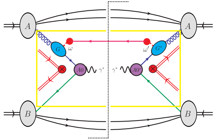
Figure 2: Graphical representation of the factorization theorem in Eq. (2.34), valid for the $g\bar{q}$ channel in Drell-Yan near threshold at NLP. In this picture red lines represent soft fields, blue lines represent collinear fields, and green lines are anti-collinear fields. The purple circles denoted by “$A0$” and “$A0^{*}$” represent the leading power short-distance coefficient $C^{A0}(Q^{2})$ and its complex conjugate, respectively. The blue ovals denoted by $G$, $G^{*}$ represents the (momentum-space representation of the) collinear functions, introduced in the matching equation Eq. (2.1). The red double lines represent the soft Wilson lines and the red filled circles are insertions of the soft quark building blocks. Last, $\omega$ and $\omega^{\prime}$ are the convolution variables between the collinear functions and the soft function.

The last simplification which can be applied when considering Eq. (2.26) up to NLP concerns the phase space integration. As discussed for the $q\bar{q}$ channel in [21], also the kinematic factors in Eq. (2.26) need to be expanded consistently to NLP: this implies that the matrix element squared expanded to NLP needs to be integrated against the LP expansion of the phase space, while the LP matrix element needs to be multiplied by the phase space expanded up to NLP. These two contributions are identified respectively as “dynamical” and “kinematic” terms: $\Delta_{\rm{NLP}}(z)=\Delta^{dyn}_{\rm NLP}(z)+\Delta^{kin}_{\rm NLP}(z)$. In case of the $g\bar{q}$ channel the matrix element squared starts at NLP, therefore there is no kinematic contribution:

$$\Delta_{g\bar{q}}(z)|_{\rm NLP}=\Delta^{dyn}_{g\bar{q}}(z)|_{\rm NLP}\,.$$ (2.32)

Taking the LP approximation of the phase space implies the following replacement in Eq. (2.26):

$$\frac{1}{2z(1-\epsilon)^{2}}\int\frac{d^{d-1}\vec{q}}{(2\pi)^{3}\,2\sqrt{Q^{2}+\vec{q}^{\,2}}}\frac{Q}{2\pi}\int d^{d}x\,e^{i(p_{A}x_{a}+p_{B}x_{b}-q)\cdot x}\to\frac{1}{8\pi(1-\epsilon)^{2}}\int dx^{0}\,e^{i\frac{\Omega}{2}x^{0}}\,,$$ (2.33)

where $\Omega=Q(1-z)$. As a consequence of this approximation, we can set $\vec{x}=0$ in the argument of the position space soft function. Last, we observe that we can carry out a further simplification by setting the anticollinear function to its LP expression, $\bar{J}_{\bar{i}}\left(n_{-}\bar{p},x_{b}n_{-}p_{B};\bar{\omega}\right)=\delta(n_{-}\bar{p}-x_{b}n_{-}p_{B})$, given that the suppression to NLP is already provided by the two insertions of $\mathcal{L}^{(1)}_{\xi q}$.

Applying all these simplifications to Eq. (2.26) we finally get

$$\Delta_{g\bar{q}}|_{\rm NLP}(z)=8H(Q^{2})\,\int{d\omega}\,d\omega^{\prime}\,G^{*}_{\xi q}(x_{a}n_{+}p_{A};\omega^{\prime})\,G_{\xi q}(x_{a}n_{+}p_{A};\omega)\,S(\Omega,\omega,\omega^{\prime})\,,$$ (2.34)

where the hard function is also given by the LP approximation of the LP short-distance coefficient squared: $H(\hat{s})=|C^{A0,A0}(x_{a}n_{+}p_{A},x_{b}n_{-}p_{B})|^{2}=H(Q^{2})+\mathcal{O}(\lambda^{2})$, and the soft function ${S}(\Omega,\omega,\omega^{\prime})$ is given by

$$S_{g\bar{q}}(\Omega,\omega,\omega^{\prime}) = \int\frac{dx^{0}}{4\pi}\int\frac{dz_{-}}{2\pi}\int\frac{dz^{\prime}_{-}}{2\pi}e^{-i\omega z_{-}}e^{+i\omega^{\prime}z^{\prime}_{-}}e^{+i\,\Omega\,x^{0}/2}$$ (2.35)

$$\times\frac{1}{N_{c}^{2}-1}\langle 0|\bar{T}\Big{(}\frac{g_{s}}{in_{-}\partial_{z^{\prime}}}\bar{q}^{\,+}(x^{0}+z^{\prime}_{-})\,\mathbf{T}^{A}\,\big{\{}Y^{\dagger}_{+}(x^{0})Y_{-}(x^{0})\big{\}}\Big{)}$$

$$\times\frac{\not{n}_{-}}{4}T\Big{(}\left\{Y^{\dagger}_{-}(0)Y_{+}(0)\right\}\,\mathbf{T}^{A}\,\frac{g_{s}}{in_{-}\partial_{z}}q^{+}(z_{-})\Big{)}|0\rangle\,.$$

The $\mathcal{L}^{(1)}_{\xi q}$ insertion in the amplitude is at position $z_{-}$, whereas in the conjugate amplitude we place the same insertion at position $z^{\prime}_{-}$. The conjugate variables to these coordinate-space variables are $\omega$ and $\omega^{\prime}$ respectively. A graphical representation of the factorization theorem in Eq. (2.34) is given in Fig. 2. We note that the factorization formula in Eq. (2.34), in the same way as the results for the $q\bar{q}$-channel Drell-Yan cross-section, is formally valid in $d$-dimension. The objects appearing in the factorization formula, ${G}_{\xi q}(x_{a}n_{+}p_{A};\omega)$, ${G}^{*}_{\xi q}(x_{a}n_{+}p_{A};\omega^{\prime})$, and ${S}_{g\bar{q}}(\Omega,\omega,\omega^{\prime})$, should not be treated as renormalized objects, because the convolution linking the collinear and soft functions must be performed in $d$-dimensions. We stress that the factorization formula in Eq. (2.34) is valid at the level of the partonic cross section. In particular, in the context of SCET, it was argued in [7] that Glauber modes give scaleless contributions at partonic level and therefore Glauber fields are not included in the construction of the effective theory. In the next two sections we compute the collinear and soft functions, respectively to ${\mathcal{O}}(\alpha_{s})$ and ${\cal O}(\alpha_{s}^{2})$, which is necessary to achieve NNLO accuracy for the invariant mass distribution.

3 Collinear functions

We now proceed to calculate the collinear function $G_{\xi q}(x_{a}n_{+}p_{A};\omega)$ up to one loop, by means of the matching equation (2.28). Before continuing, let us notice that an equivalent collinear function has been defined in the context of $H\to gg$ in [52], which has been calculated up to two loops. We provide here an independent calculation and check that our result for the one-loop collinear function defined in Eq. (2.28) is indeed equivalent to the one considered in [52]. In order to set-up the calculation it proves useful to introduce the short-hand notation

$$\tilde{\mathcal{T}}_{\gamma f}(t) \equiv i\int d^{4}z\,T\Big{[}\chi_{c,\gamma f}\left(tn_{+}\right)\mathcal{L}^{(1)}_{\xi q}(z)\Big{]}\,,$$ (3.1)

for the left-hand side of (2.28). We then consider its Fourier transform

$$\mathcal{T}_{\gamma f}(n_{+}q) =\int dt\,e^{i(n_{+}q)\,t}\,\tilde{\mathcal{T}}_{\gamma f}(t)\,,$$ (3.2)

and rewrite the matching equation (2.28) in momentum space as follows

$$\mathcal{T}_{\gamma f}(n_{+}q) = 2\pi\int\frac{dn_{+}p_{a}}{2\pi}\int du\,e^{i\,(n_{+}p_{a})\,u}\,\int\frac{d\omega}{2\pi}$$ (3.3)

$$\times{G}^{\,\eta,A}_{\xi q;\gamma\alpha,fa}\left(n_{+}q,n_{+}p_{a};\omega\right)\,\frac{1}{g_{s}}{\mathcal{A}}^{{\rm PDF}\,A}_{c\perp\eta}(un_{+})\int dz_{-}\,e^{-i\omega\,z_{-}}\,\mathfrak{s}_{\xi q;\alpha,a}(z_{-})\,.$$

Starting from this definition, we extract the perturbative collinear functions by considering suitable partonic matrix elements of the operator matching equation. In this case, the relevant matrix element involves an incoming $c$-PDF gluon and an outgoing soft quark $\langle q^{+}(k)|...|g(p)\rangle$. We compute both sides of the matching equation with the leading power decoupled Lagrangian, considering the soft fields as external. Hence, we only need the soft matrix element $\langle q^{+}(k)|\mathfrak{s}_{\xi q;\alpha,a}(z_{-})|0\rangle$ at tree level. Similarly, for the $c$-PDF matrix element $\langle 0|{\mathcal{A}}^{{\rm PDF}\,A}_{c\perp\eta}(un_{+})|g(p)\rangle$ the loop corrections are scaleless and $\langle 0|{\mathcal{A}}^{{\rm PDF}\,A}_{c\perp\eta}(un_{+})|g(p)\rangle$ contributes only at tree level. The calculation of the left-hand side of Eq. (3.3) is done using the momentum-space Feynman rules given in appendix A of [59]. Before moving to the description of the actual calculation, we point out that this calculation is far more straightforward compared to the case of the corresponding collinear functions in the $q\bar{q}$ channel, see [21]. This is because, as discussed above, we need to consider the single soft structure given in Eq. (2.29); furthermore, the Lagrangian insertion $\mathcal{L}^{(1)}_{\xi q}$ which induces the power suppression does not contain any explicit position variables, which means that, in momentum space, no derivatives on the momentum conserving delta functions appear at subleading power soft-collinear interaction vertices. This reduces drastically the number of terms which appear in each diagram and the number of integrals involved in the calculation.

3.1 Tree-level collinear function

We first consider the right-hand side of (3.3) and evaluate the tree-level matrix element

$$\langle q^{+}_{b}(k)|\mathcal{T}_{\gamma f}(n_{+}q)|g^{B}(p)\rangle = 2\pi\int\frac{dn_{+}p_{a}}{2\pi}\int du\,e^{i\,(n_{+}p_{a})\,u}\,\int\frac{d\omega}{2\pi}\int dz_{-}\,e^{-i\omega\,z_{-}}$$ (3.4)

$$\times{G}^{\,\eta,A}_{\xi q;\gamma\alpha,fa}\left(n_{+}q,n_{+}p_{a};\omega\right)\,\langle 0|\frac{1}{g_{s}}{\mathcal{A}}^{{\rm PDF}\,A}_{c\perp\eta}(un_{+})|g^{B}(p)\rangle\,\langle q^{+}_{b}(k)|\mathfrak{s}_{\xi q;\alpha,a}(z_{-})|0\rangle\,,$$

where $B$ is the adjoint color index and $b$ is the fundamental color index of the external final state. The $c$-PDF matrix element in (3.4) evaluates to the following

$$\langle 0|\frac{1}{g_{s}}{\mathcal{A}}^{{\rm PDF}\,A}_{c\perp\eta}(un_{+})|g^{B}(p)\rangle=\delta^{AB}\,\sqrt{Z_{g,{\rm{PDF}}}}\,\epsilon_{{\perp}\eta}(p)\,e^{-i(n_{+}p)u}.$$ (3.5)

The factor $\sqrt{Z_{g,{\rm{PDF}}}}$ is the on-shell renormalization factor of the $c$-PDF gluon field. The soft matrix element on the right-hand side of (3.4) becomes

$$\langle q^{+}_{b}(k)|\mathfrak{s}_{\xi q;\alpha,a}(z_{-})|0\rangle=\langle q^{+}_{b}(k)|\frac{g_{s}}{in_{-}\partial_{z}}q^{+}_{\alpha,a}(z_{-})|0\rangle=-\delta_{ba}\,\frac{g_{s}}{n_{-}k}\,v_{\alpha}(k)\,e^{iz_{-}\cdot k}\,.$$ (3.6)

In the second step we have used the form of the soft structure as given in Eq. (2.29). As originally discussed below Eq. (4.3) of [21] for the case of collinear functions involving PDF and threshold quarks, the matrix elements in Eqs. (3.5) and (3.6) do not have loop corrections. This is true in Eq. (3.5) because the loop corrections are scaleless, and it also holds for Eq. (3.6) because here the soft field is treated as external. Next, we substitute the matrix elements evaluated in Eqs. (3.5) and (3.6) into (3.4) and find

$$\langle q^{+}_{b}(k)|\mathcal{T}_{\gamma f}(n_{+}q)|g^{B}(p)\rangle = -(2\pi)\frac{g_{s}}{n_{-}k}\,{G}^{\,\eta,B}_{\xi q;\gamma\alpha,fb}\left(n_{+}q,n_{+}p;n_{-}k\right)\,$$ (3.7)

$$\times\,v_{\alpha}(k)\,\sqrt{Z_{g,{\rm{PDF}}}}\,\epsilon_{{\perp}\eta}(p)\,.$$

This result constitutes the final expression for the matrix element with the chosen partonic external states of the right-hand side of the matching equation in (3.3). Since the matrix elements in Eqs. (3.5) and (3.6) have no loop corrections, the expression in Eq. (3.7) is valid to all orders in $\alpha_{s}$.

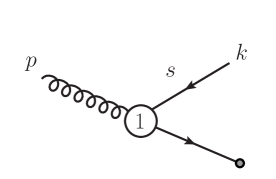
Figure 3: Tree-level EFT diagram in the $g\bar{q}$-channel.

Having obtained an expression for the right-hand side of the matching equation (3.4), we now compute the left-hand side, which corresponds to the diagram in Fig. 3. The Lagrangian insertion in Eq. (3.1) can be computed by means of the Feynman rule given in Eq. (A.36) of [59] and we obtain

$$\langle q^{+}_{b}(k)|\mathcal{T}_{\gamma f}(n_{+}q)|g^{B}(p)\rangle = (2\pi)\delta(n_{+}q-n_{+}p)\frac{1}{n_{-}k}\,g_{s}\mathbf{T}^{B}_{fb}$$ (3.8)

$$\times\,\left(\frac{\not{n}_{-}}{2}\gamma_{\perp{\eta}}\right)_{\gamma\alpha}\,v_{\alpha}(k)\sqrt{Z_{g,c}}\rvert_{{\rm{tree}}}\epsilon^{\eta}_{\perp}(p)+\mathcal{O}(\alpha_{s})\,.$$

The tree-level value of the on-shell wave function renormalization factor of the gluon field is $\sqrt{Z_{g,c}}\rvert_{{\rm{tree}}}=1$ in the EFT.

Since at next-to-leading power in the $g\bar{q}$-channel only a single soft structure is relevant, no additional manipulations relating to the use of equation-of-motion identity, or on-shell and transversality conditions are necessary here, in contrast to the calculation of the collinear functions for the $q\bar{q}$-channel, see section 4.1 of [21]. At this point, we simply compare the result for the left-hand side of the matching equation given in Eq. (3.8) to the right-hand side in Eq. (3.7) and read off the tree-level result for the collinear function

$${G}^{\,\eta,B}_{\xi q;\gamma\alpha,fb}\left(n_{+}q,n_{+}p;\omega\right)=-\,\delta(n_{+}q-n_{+}p)\,\mathbf{T}^{B}_{fb}\,\left(\frac{\not{n}_{-}}{2}\gamma_{\perp{\eta}}\right)_{\gamma\alpha}+\mathcal{O}(\alpha_{s})\,.$$ (3.9)

Using the decomposition introduced in Eq. (2.30) we can extract the scalar collinear function ${G}_{\xi q}(n_{+}p;\omega)$ which appears in the factorization formula in (2.34). Namely, we find

$${G}^{(0)}_{\xi q}(n_{+}p;\omega)=-\frac{1}{2}\,,$$ (3.10)

where the superscript $(0)$ denotes the tree-level result.

3.2 One-loop collinear function

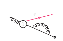
(a)

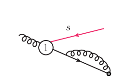
(b)

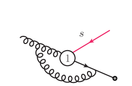
(c)

(d)

(e)

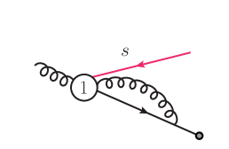
(f)

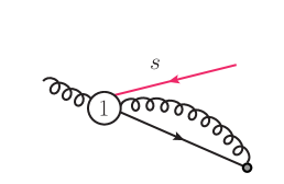
(g)

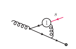
(h)

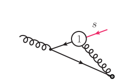
(i)

Figure 4: One-loop diagrams contributing to the collinear function.

We are now ready to consider the $\mathcal{O}(\alpha_{s})$ correction. For the right-hand side of the matching we use Eq. (3.7). Here the on-shell wave function renormalization factor is unity to all orders in perturbation theory: $\sqrt{Z_{g,{\rm{PDF}}}}=1$. This holds in dimensional regularization, which we use to treat infrared and ultraviolet divergences, since the loop corrections are scaleless. The situation is the same for the $\sqrt{Z_{g,c}}$ factor on the left-hand side of the matching equation, see Eq. (3.8). Given that the calculation is relatively straightforward, we skip the details of the computation and present the results for the one-loop matrix element $\langle q^{+}_{b}(k)|\mathcal{T}_{\gamma f}(n_{+}q)|g^{B}(p)\rangle$ on the left-hand side of the matching equation (3.3), which is given by the sum over the one loop diagrams represented in Fig. 4 (a) – (i). Let us only notice that diagram (e), (g) and (i) are zero, the latter because the collinear loop does not have a scale. Furthermore, diagrams (a) and (b) contribute with a color factor $C_{F}$, (c) and (d) with a color factor $(-C_{A}/2)$, (h) and (f) are proportional to $(C_{F}-C_{A}/2)$. We obtain

$$\langle q^{+}_{b}(k)|\mathcal{T}_{\gamma f}(n_{+}q)|g^{B}(p)\rangle^{(1)} = (2\pi)\delta(n_{+}q-n_{+}p)\,\frac{\alpha_{s}}{4\pi}\,g_{s}\,\mathbf{T}^{B}_{fb}\big{(}C_{F}-C_{A}\big{)}\bigg{(}\frac{n_{+}p\,n_{-}k}{\mu^{2}}\bigg{)}^{-\epsilon}$$ (3.11)

$$\times\,\frac{e^{\epsilon\gamma_{E}}\Gamma[1+\epsilon]\Gamma[1-\epsilon]^{2}}{\Gamma[2-2\epsilon]}\,\frac{2-4\epsilon-\epsilon^{2}}{\epsilon^{2}}\,\frac{1}{n_{-}k}\left(\frac{\not{n}_{-}}{2}\gamma_{\perp{\eta}}\right)_{\gamma\alpha}v_{\alpha}(k)\,\epsilon^{\eta}_{\perp}(p)\,,$$

where the superscript (1) on the left-hand side indicates that the matrix element is considered at order $\alpha_{s}$. We match this result to the right-hand side of Eq. (3.7), from which we extract the perturbative matching coefficient, the collinear function, at one-loop order

$${G}^{\,\eta,B\,(1)}_{\xi q;\gamma\alpha,fb}\left(n_{+}q,n_{+}p;\omega\right) = -\,\frac{\alpha_{s}}{4\pi}\,\mathbf{T}^{B}_{fb}\big{(}C_{F}-C_{A}\big{)}\left(\frac{n_{+}p\,\omega}{\mu^{2}}\right)^{-\epsilon}\frac{2-4\epsilon-\epsilon^{2}}{\epsilon^{2}}$$ (3.12)

$$\times\frac{e^{\epsilon\gamma_{E}}\Gamma[1+\epsilon]\Gamma[{1-\epsilon}]^{2}}{\Gamma[{2-2\epsilon}]}\left(\frac{\not{n}_{-}}{2}\gamma_{\perp}^{\eta}\right)_{\gamma\alpha}\delta(n_{+}q-n_{+}p)\,.$$

Using the decomposition introduced in Eq. (2.30), the scalar collinear function ${G}_{\xi q}(n_{+}p;\omega)$ at one loop reads

$${G}^{(1)}_{\xi q}\left(n_{+}p;\omega\right)=-\,\frac{\alpha_{s}}{4\pi}\big{(}C_{F}-C_{A}\big{)}\left(\frac{n_{+}p\,\omega}{\mu^{2}}\right)^{-\epsilon}\frac{2-4\epsilon-\epsilon^{2}}{2\epsilon^{2}}\frac{e^{\epsilon\gamma_{E}}\Gamma[1+\epsilon]\Gamma[{1-\epsilon}]^{2}}{\Gamma[{2-2\epsilon}]}\,.$$ (3.13)

This is the $\mathcal{O}(\alpha_{s})$ correction to the tree-level collinear function presented in Eq. (3.10), valid to all orders in $\epsilon$. As anticipated it agrees with the result given in [52], see in particular Eqs. (1.4), (2.1) and (2.3) there, apart from an overall normalization factor $\propto 1/\omega$, that by definition we shuffle into the soft function such as to define a dimensionless collinear function. Expanding Eq. (3.13) in $\epsilon=(4-d)/2$ we arrive at

$${G}^{(1)}_{\xi q}\left(n_{+}p;\omega\right) = -\,\frac{\alpha_{s}}{4\pi}\big{(}C_{F}-C_{A}\big{)}\bigg{[}\frac{1}{\epsilon^{2}}-\frac{1}{\epsilon}\ln\left(\frac{n_{+}p\,\omega}{\mu^{2}}\right)$$ (3.14)

$$\hskip 85.35826pt-\,\frac{1}{2}-\frac{\pi^{2}}{12}+\frac{1}{2}\ln^{2}\left(\frac{n_{+}p\,\omega}{\mu^{2}}\right)+\mathcal{O}(\epsilon)\bigg{]}\,.$$

It is interesting to compare the above result for the collinear function appearing in the $g\bar{q}$-channel to the collinear functions in the $q\bar{q}$-channel, which have been given in their expanded form in equations (4.31) and (4.34) of [21]. We note that here, in contrast to $J_{1}^{(1)}$ and $J_{6}^{(1)}$, the collinear function ${G}^{(1)}_{\xi q}$ exhibits $1/\epsilon^{2}$ poles, and finite logarithms $\propto\,\ln^{2}(n_{+}p\,\omega/\mu^{2})$. At cross-section level, as we will show in section 5 below, these correspond to leading logarithmic contributions appearing in the collinear sector. This fact complicates the adaptation of the resummation treatment developed for the $q\bar{q}$-channel [20] to the off-diagonal $g\bar{q}$-channel. We provide additional details in section 5. It is noteworthy that the leading pole structure in the above equation is proportional to $C_{F}-C_{A}$. As discussed in several instances in literature, cf. [66, 67, 68, 26, 29, 32], this structure characterizes the conversion of a collinear gluon into a collinear quark by means of an emission of a soft-quark; its factorization into soft and collinear parts typically involves divergent convolution integrals.

4 Soft functions

The last ingredient needed to reproduce the partonic cross section up to NNLO in perturbation theory are the one and two-loop soft function defined in Eq. (2.35), that we calculate in this section. To this end it is useful to insert a complete set of states between the ${\bar{T}}$ and ${T}$ products, and use the momentum operator to translate the fields in the anti-time-ordered part. Performing the integration over $x^{0}$ in Eq. (2.35) gives rise to an energy conserving delta function. Writing spinor and color indices explicitly one has

$$S_{g\bar{q}}(\Omega,\omega,\omega^{\prime}) = \sum_{X_{s}}\int\frac{dz_{-}}{2\pi}\int\frac{dz^{\prime}_{-}}{2\pi}e^{-iz_{-}\omega}e^{+iz^{\prime}_{-}\omega^{\prime}}\delta(\Omega-2E_{X_{s}})$$ (4.1)

$$\times\,\frac{1}{N_{c}^{2}-1}\langle 0|\bar{T}\Big{(}\frac{g_{s}}{in_{-}\partial_{z^{\prime}}}\bar{q}^{\,+}_{\sigma k}(z^{\prime}_{-})({\bf T}^{D})_{kl}\big{\{}Y^{\dagger}_{+}(0)Y_{-}(0)\big{\}}_{la}\Big{)}|X_{s}\rangle$$

$$\times\,\frac{\not{n}_{-\sigma\beta}}{4}\langle X_{s}|T\Big{(}\big{\{}Y^{\dagger}_{-}(0)Y_{+}(0)\big{\}}_{af}({\bf T}^{D})_{fj}\frac{g_{s}}{in_{-}\partial_{z}}q^{+}_{\beta j}(z_{-})\Big{)}|0\rangle.$$

In what follows we evaluate the soft function at first and second order in $\alpha_{s}$, which is indicated below by a superscript $(1)$ and $(2)$, respectively.

4.1 First order

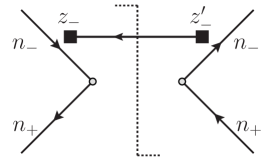
Figure 5: Diagram contributing to the soft function at first order (NLO in $\alpha_{s}$).

At one loop the final state contains a single soft quark and the matrix element reads

$$\langle q_{s,e}(k)|T\Big{(}\big{\{}Y^{\dagger}_{-}(0)Y_{+}(0)\big{\}}_{af}({\bf T}^{D})_{fj}\frac{g_{s}}{in_{-}\partial_{z}}q^{+}_{\beta j}(z_{-})\Big{)}|0\rangle=\frac{g_{s}({\bf T}^{D})_{ae}}{-n_{-}k}\,v_{s,\beta}(k)\,e^{iz_{-}\cdot k}+\mathcal{O}(g_{s}^{3}),$$ (4.2)

The complex-conjugate matrix element can be derived accordingly. Inserting these into Eq. (4.1) and introducing the notation

$$\int[dk]\equiv\left(\frac{\mu^{2}e^{\gamma_{E}}}{4\pi}\right)^{\epsilon}\int\frac{d^{d}k}{(2\pi)^{d}},$$ (4.3)

we easily get

$$S_{g\bar{q}}^{(1)}(\Omega,\omega,\omega^{\prime}) = 2\pi\,g_{s}^{2}\,T_{F}\int[dk]\,\frac{\delta^{+}(k^{2})}{n_{-}k}\delta(\omega-n_{-}k)\delta(\omega^{\prime}-n_{-}k)\delta(\Omega-n_{+}k-n_{-}k)$$ (4.4)

$$= \frac{\alpha_{s}\,T_{F}}{4\pi}\frac{e^{\epsilon\gamma_{E}}}{\Gamma[1-\epsilon]}\frac{1}{\omega}\bigg{(}\frac{\mu^{2}}{\omega\,(\Omega-\omega)}\bigg{)}^{\epsilon}\delta(\omega-\omega^{\prime})\,\theta(\Omega-\omega)\theta(\omega),$$

which we express in terms of the color factor ${\rm Tr}[{\bf T}^{A}{\bf T}^{B}]=T_{F}\,\delta^{AB}=\delta^{AB}/2$, characteristic of the quark-gluon channel.

4.2 Second order: virtual-real contribution

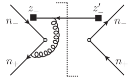
(a)

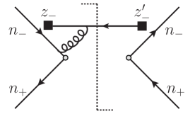
(b)

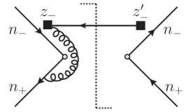
(c)

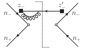
(d)

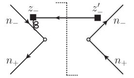
(e)

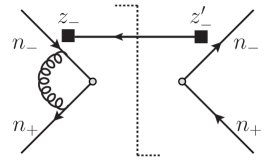
(f)

Figure 6: Diagrams contributing to the virtual-real part of the soft function at second order in $\alpha_{s}$. The part to the left (right) of the cut corresponds to the time-ordered (anti-time-ordered) part of the diagram, and lines labeled by $n_{\pm}$ with in (out)-going arrow correspond to soft Wilson lines $Y_{\mp}$($Y_{\mp}^{\dagger}$). The filled square in this figure stands for the soft quarks and the Wilson lines contained in $q^{+}=Y^{\dagger}_{+}q_{s}$.

At second order in $\alpha_{s}$ we need to take into account two different types of corrections: the virtual-real contribution, involving a soft gluon loop in the matrix element (or in the complex conjugate one) and the real-real contribution, involving the emission of a soft gluon in addition to the soft anti-quark. We start by considering the virtual-real contribution. The one-loop matrix element is given by

$$\langle q_{s,e}(k_{1})|T\Big{(}\big{\{}Y^{\dagger}_{-}(0)Y_{+}(0)\big{\}}_{af}({\bf T}^{D})_{fj}\frac{g_{s}}{in_{-}\partial_{z}}q^{+}_{\beta j}(z_{-})\Big{)}|0\rangle$$ (4.5)

$$=\,i\,g_{s}^{3}\,({\bf T}^{D})_{ae}\int[dk]\bigg{\{}C_{F}\,\frac{2}{k^{2}(n_{+}k)(-n_{-}k)(-n_{-}k_{1})}e^{iz_{-}\cdot k_{1}}$$

$$-\,\bigg{(}C_{F}-\frac{C_{A}}{2}\bigg{)}\frac{2}{k^{2}(n_{+}k)(-n_{-}k)(-n_{-}k-n_{-}k_{1})}e^{iz_{-}\cdot k_{1}}$$

$$-\,\bigg{(}C_{F}-\frac{C_{A}}{2}\bigg{)}\frac{(\not{k}+\not{k}_{1})\not{n}_{+}}{k^{2}(k+k_{1})^{2}(n_{-}k)(-n_{-}k-n_{-}k_{1})}e^{iz_{-}\cdot(k_{1}+k)}$$

$$+\,\bigg{(}C_{F}-\frac{C_{A}}{2}\bigg{)}\frac{(\not{k}+\not{k}_{1})\not{n}_{-}}{k^{2}(k+k_{1})^{2}(n_{-}k)(-n_{-}k-n_{-}k_{1})}e^{iz_{-}\cdot(k_{1}+k)}$$

$$-\,C_{F}\,\frac{(\not{k}+\not{k}_{1})\not{n}_{-}}{k^{2}(k+k_{1})^{2}(n_{-}k)(-n_{-}k_{1})}e^{iz_{-}\cdot k_{1}}\bigg{\}}\,v_{s,\beta}(k_{1})\,+\mathcal{O}(g_{s}^{5}),$$

where linear propagators are written such that they carry a small positive imaginary factor $+i0_{+}$, and the terms on the right-hand side represent respectively Fig. 6 (f), (c), (a), (b), (d), while (e) is immediately zero. Among these, it turns out that only diagram (c) contributes. We focus on this term and insert the matrix element in Eq. (4.1) with the complex conjugate matrix element taken at lowest order; furthermore, we recall that we need to take into account also the complex conjugate one-loop matrix element times the tree level matrix element, such that the full contribution to the virtual-real part of the soft function reads

$$S^{(2)1r1v}_{g\bar{q}}(\Omega,\omega,\omega^{\prime}) = {\rm Re}\bigg{\{}i\,g_{s}^{4}\,T_{F}(2C_{F}-C_{A})\int[dk_{1}]\int[dk]$$ (4.6)

$$\times\,(2\pi)\delta(k_{1}^{2})\theta(k_{1}^{0})\,\delta(\Omega-2k_{1}^{0})\,\delta(\omega^{\prime}-n_{-}k_{1})\delta(\omega-n_{-}k-n_{-}k_{1})$$

$$\times\,\frac{(k+k_{1})^{2}-k^{2}+n_{-}k_{1}(n_{+}k+n_{+}k_{1})+n_{+}k_{1}(n_{-}k+n_{-}k_{1})}{k^{2}(k+k_{1})^{2}(n_{+}k)(-n_{-}k-n_{-}k_{1})(-n_{-}k_{1})}\,\bigg{\}}.$$

We evaluate the integrations over $k$ and $k_{1}$ following two independent approaches: within the first, we integrate directly the terms appearing in Eq. (4.6); within the second we first reduce such terms to a basis of master integrals, in which case Eq. (4.6) reads

$$S^{(2)1r1v}_{g\bar{q}}(\Omega,\omega,\omega^{\prime})={\rm Re}\bigg{\{}-i\,\frac{\alpha_{s}^{2}\,T_{F}}{(4\pi)^{2}}(2C_{F}-C_{A})\bigg{[}\frac{1}{\omega\omega^{\prime}}\hat{J}_{1}+\frac{(\omega+\omega^{\prime})(\Omega-\omega^{\prime})}{\omega\omega^{\prime}}\hat{J}_{2}\bigg{]}\bigg{\}},$$ (4.7)

where the master integrals $\hat{J}_{i}$ are defined in Eq. (A.3) and calculated in Eqs. (A.4) and (A.1) of appendix A.1. Using the results given there we get

$$S^{(2)1r1v}_{g\bar{q}}(\Omega,\omega,\omega^{\prime}) = \frac{\alpha_{s}^{2}\,T_{F}}{(4\pi)^{2}}(2C_{F}-C_{A})\frac{e^{2\epsilon\gamma_{E}}\,\Gamma[1+\epsilon]}{\epsilon\,\Gamma[1-\epsilon]}$$ (4.8)

$$\times\,{\rm Re}\bigg{\{}\frac{1}{(-\omega)\omega^{\prime}}\bigg{[}\frac{\omega+\omega^{\prime}}{\omega^{\prime}}\,_{2}F_{1}\bigg{(}1,1+\epsilon,1-\epsilon,\frac{\omega}{\omega^{\prime}}\bigg{)}-1\bigg{]}\bigg{(}\frac{\mu^{4}}{(-\omega)\omega^{\prime}(\Omega-\omega^{\prime})^{2}}\bigg{)}^{\epsilon}\theta(-\omega)$$

$$+\,\frac{2(\omega+\omega^{\prime})}{\omega\omega^{\prime}(\omega^{\prime}-\omega)}\bigg{(}\frac{\mu^{4}}{(\omega^{\prime}-\omega)^{2}(\Omega-\omega^{\prime})^{2}}\bigg{)}^{\epsilon}\frac{\Gamma[1-\epsilon]^{2}}{\Gamma[1-2\epsilon]}\theta(\omega^{\prime}-\omega)\bigg{\}}\theta(\omega^{\prime})\theta(\Omega-\omega^{\prime}).$$

4.3 Second order: real-real contribution

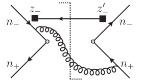
(a)

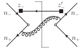
(b)

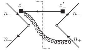
(c)

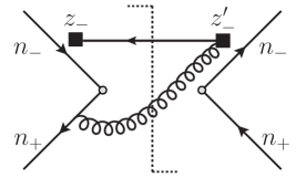
(d)

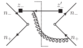
(e)

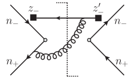
(f)

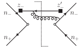
(g)

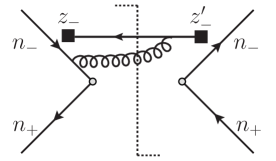
(h)

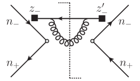
(i)

Figure 7: Diagrams contributing to the real-real part of the soft function. The part to the left (right) of the cut corresponds to the time-ordered (anti-time-ordered) part of the diagram, and lines labeled by $n_{\pm}$ with in (out)-going arrow correspond to soft Wilson lines $Y_{\mp}$($Y_{\mp}^{\dagger}$). The filled square in this figure stands for the soft quarks and the Wilson lines contained in $q^{+}=Y^{\dagger}_{+}q_{s}$.

We consider now the final state emission of a soft gluon in addition to the soft-antiquark. The matrix element reads

$$\langle q_{s,e}(k_{1})g^{H}_{s}(k_{2})|T\bigg{(}\big{\{}Y^{\dagger}_{-}(0)Y_{+}(0)\big{\}}_{af}({\bf T}^{D})_{fj}\frac{g_{s}}{in_{-}\partial_{z}}q^{+}_{\beta j}(z_{-})\bigg{)}|0\rangle$$

$$=\,g_{s}^{2}\bigg{[}({\bf T}^{H}{\bf T}^{D})_{ae}\frac{1}{n_{-}k_{1}}\bigg{(}\frac{n_{+}\varepsilon(k_{2})}{n_{+}k_{2}}-\frac{n_{-}\varepsilon(k_{2})}{n_{-}k_{2}}\bigg{)}e^{i\,z_{-}\cdot k_{1}}$$

$$+\,({\bf T}^{D}{\bf T}^{H})_{ae}\frac{1}{n_{-}(k_{1}+k_{2})}\bigg{(}\frac{n_{+}\varepsilon(k_{2})}{n_{-}k_{2}}-\frac{(\not{k_{1}}+\not{k_{2}})\not{\varepsilon}(k_{2})}{(k_{1}+k_{2})^{2}}\bigg{)}e^{i\,z_{-}\cdot(k_{1}+k_{2})}\bigg{]}v_{s,\beta}(k_{1})+\mathcal{O}(g_{s}^{4}).$$

In practice we have four contributions: three diagrams where the gluon is taken from one of the three Wilson lines in Eq. (4.3), counting also the Wilson line implicit in $q^{+}=Y^{\dagger}_{+}q_{s}$, and the fourth where the gluon is taken from the insertion of the (leading power) soft Lagrangian ${\cal L}^{(0)}_{s}(y)=\bar{q}_{s}(y)g_{s}\not{A}_{s}(y)q_{s}(y)$. The soft function is obtained according to Eq. (4.1) where the complex conjugate matrix element can be derived from Eq. (4.3). In Fig. 7 we list the diagrams which give a non-zero contribution. We obtain

$$S^{(2)2r0v}_{g\bar{q}}(\Omega,\omega,\omega^{\prime}) = (2\pi)^{2}g_{s}^{4}\,T_{F}\,\int[dk_{1}]\int[dk_{2}]\,\delta(\Omega-2k_{1}^{0}-2k_{2}^{0})$$ (4.10)

$$\times\,\delta(k_{1}^{2})\theta(k_{1}^{0})\,\delta(k_{2}^{2})\theta(k_{2}^{0})\,\bigg{\{}C_{F}\bigg{[}-\frac{4}{n_{-}k_{1}\,n_{-}k_{2}\,n_{+}k_{2}}\delta(\omega-n_{-}k_{1})\delta(\omega^{\prime}-n_{-}k_{1})$$

$$\hskip 56.9055pt-\frac{1}{(k_{1}+k_{2})^{2}}\bigg{(}\frac{4n_{-}k_{1}}{n_{-}k_{2}\,n_{-}(k_{1}+k_{2})}+\frac{2(1-\epsilon)\,n_{-}k_{2}}{[n_{-}(k_{1}+k_{2})]^{2}}\bigg{)}$$

$$\hskip 85.35826pt\times\,\delta(\omega-n_{-}k_{1}-n_{-}k_{2})\delta(\omega^{\prime}-n_{-}k_{1}-n_{-}k_{2})\bigg{]}$$

$$+\,\bigg{(}C_{F}-\frac{C_{A}}{2}\bigg{)}\bigg{[}\frac{2}{n_{-}(k_{1}+k_{2})\,n_{-}k_{2}\,n_{+}k_{2}}+\frac{1}{n_{-}k_{1}\,n_{-}(k_{1}+k_{2})\,n_{+}k_{2}}$$

$$\hskip 56.9055pt-\frac{n_{+}k_{1}}{n_{-}k_{1}\,n_{+}k_{2}\,(k_{1}+k_{2})^{2}}-\frac{n_{+}(k_{1}+k_{2})}{n_{-}(k_{1}+k_{2})\,n_{+}k_{2}\,(k_{1}+k_{2})^{2}}$$

$$\hskip 56.9055pt+\,\frac{2}{(k_{1}+k_{2})^{2}\,n_{-}k_{2}}\bigg{]}\Big{[}\delta(\omega-n_{-}k_{1})\delta(\omega^{\prime}-n_{-}k_{1}-n_{-}k_{2})$$

$$\hskip 85.35826pt+\,\delta(\omega^{\prime}-n_{-}k_{1})\delta(\omega-n_{-}k_{1}-n_{-}k_{2})\Big{]}\bigg{\}}.$$

As for the virtual-real contribution, we evaluate the integrals over $k_{1}$ and $k_{2}$ both by directly integrating the expression in Eq. (4.10), and by reducing such expression to a basis of master integrals, in which case Eq. (4.10) becomes

$$S^{(2)2r0v}_{g\bar{q}}(\Omega,\omega,\omega^{\prime})$$ (4.11)

$$=\,\frac{\alpha_{s}^{2}}{(4\pi)^{2}}T_{F}\bigg{[}C_{F}\bigg{(}\frac{(4-\epsilon)(1-\epsilon)(1-2\epsilon)}{\epsilon^{2}\omega^{2}(\Omega-\omega)}\,\hat{I}_{6}+\frac{4(2-3\epsilon)(1-3\epsilon)}{\epsilon^{2}\omega(\Omega-\omega)^{2}}\,\hat{I}_{5}\bigg{)}\delta(\omega-\omega^{\prime})$$

$$+\,(C_{A}-2C_{F})\bigg{(}\frac{(1-2\epsilon)(\omega+\omega^{\prime})}{\epsilon\,\omega\omega^{\prime}(\Omega-\omega)(\omega-\omega^{\prime})}\,\hat{I}_{3}-\frac{(1-2\epsilon)(\omega+\omega^{\prime})}{\epsilon\,\omega\omega^{\prime}(\Omega-\omega^{\prime})(\omega-\omega^{\prime})}\,\hat{I}_{1}$$

$$\hskip 56.9055pt+\,\frac{(\Omega-\omega)(\omega+\omega^{\prime})}{2\omega\omega^{\prime}}\hat{I}_{4}+\frac{(\Omega-\omega^{\prime})(\omega+\omega^{\prime})}{2\omega\omega^{\prime}}\hat{I}_{2}\bigg{)}\bigg{]}.$$

The master integrals $\hat{I}_{i}$ are defined and evaluated in appendix A.2. After substituting the expressions for the master integrals in Eqs. (A.2)–(A.17) we finally obtain

$$S^{(2)2r0v}_{g\bar{q}}(\Omega,\omega,\omega^{\prime}) = \frac{\alpha_{s}^{2}T_{F}}{(4\pi)^{2}}\bigg{\{}C_{F}\frac{e^{2\epsilon\gamma_{E}}\Gamma[1-\epsilon]}{\epsilon^{2}}\frac{1}{\omega}\bigg{[}\frac{4}{\Gamma[1-3\epsilon]}\bigg{(}\frac{\mu^{4}}{\omega(\Omega-\omega)^{3}}\bigg{)}^{\epsilon}$$

$$+\,\frac{(4-\epsilon)\Gamma[2-\epsilon]}{(1-2\epsilon)\Gamma[1-2\epsilon]^{2}}\bigg{(}\frac{\mu^{4}}{\omega^{2}(\Omega-\omega)^{2}}\bigg{)}^{\epsilon}\bigg{]}\delta(\omega-\omega^{\prime})\theta(\Omega-\omega)\theta(\omega)$$

$$+\,\left(C_{A}-2C_{F}\right)\frac{2e^{2\epsilon\gamma_{E}}}{\epsilon\Gamma[1-2\epsilon]}\frac{\omega+\omega^{\prime}}{\omega\omega^{\prime}(\omega^{\prime}-\omega)}\bigg{(}\frac{\mu^{4}}{\omega(\omega^{\prime}-\omega)(\Omega-\omega^{\prime})^{2}}\bigg{)}^{\epsilon}$$

$$\times\,\bigg{[}\,_{2}F_{1}\Big{(}1,-\epsilon,1-\epsilon,\frac{\omega}{\omega-\omega^{\prime}}\Big{)}-1\bigg{]}\theta(\omega)\theta(\omega^{\prime})\theta(\omega^{\prime}-\omega)\theta(\Omega-\omega^{\prime})\bigg{\}}.$$

Eqs. (4.8) and (4.3) provide the complete result for the two-loop soft function.

4.4 Asymptotic limits

With the results of the NNLO soft function calculation at hand, we now have the opportunity to study the asymptotic limits of this object. This is useful, because endpoint divergences arise exactly in these limits, thus understanding the emergent asymptotic structure of the soft function is useful for any future study of endpoint refactorization. Indeed, as shown for instance for the off-diagonal “gluon” thrust in [32], the asymptotic limits of the soft (and collinear) functions are the objects one needs to subtract from the full functions, in order to define matrix elements free of endpoint divergences. After this procedure has been completed, it is then possible to implement the standard resummation procedure, based on the renormalization-group evolution of the subtracted functions.

At NLO the soft function is relatively simple, and inspecting Eq. (4.4) we see that an endpoint divergence arises for $\omega,\omega^{\prime}\to 0$:

$$S(\Omega,\omega,\omega^{\prime},\mu)|_{\omega,\omega^{\prime}\to 0}=\frac{\alpha_{s}\,T_{F}}{4\pi}\frac{e^{\epsilon\gamma_{E}}}{\Gamma[1-\epsilon]}\frac{1}{\omega}\bigg{(}\frac{\mu^{2}}{\omega\,\Omega}\bigg{)}^{\epsilon}\delta(\omega-\omega^{\prime})\,\theta(\Omega)\theta(\omega).$$ (4.13)

In particular, notice that, because of the factor $\delta(\omega-\omega^{\prime})$, one has effectively a dependence on a single variable $\omega$. This is analogous to the situation in [32] where the relevant asymptotic limit is $\omega,\omega^{\prime}\to\infty$, however identical simplification occurs, namely, the presence of a Dirac Delta function reduces the functional dependence of the soft function to a single $\omega$ variable (see e.g. Eq. (27) in [32]).

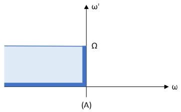
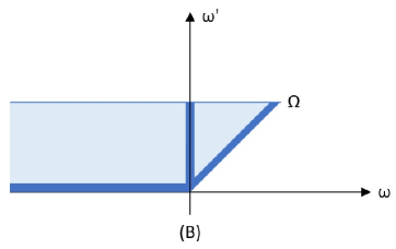
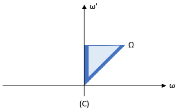
Figure 8: Integration domain for the three terms of the two-loop soft functions, defined (from left to right) respectively as $S^{(2A)}(\omega,\omega^{\prime})$, $S^{(2B)}(\omega,\omega^{\prime})$ and $S^{(2C)}(\omega,\omega^{\prime})$ in Eq. (4.14). The shaded blue areas represent endpoint regions where the integral of the soft function is divergent.

The calculation of the soft function at two loops in sections 4.2, 4.3 gives us the opportunity to explore its asymptotic limits for the first time beyond NLO. Indeed, we find a more involved structure of endpoint singularities, which arise for $\omega\to 0$, $\omega^{\prime}\to 0$ separately, as well as for $\omega^{\prime}-\omega\to 0$. To be more specific, let us write the soft function as follows:

$$S^{(2)}(\omega,\omega^{\prime}) = \hat{S}^{(2)}(\omega)\,\delta(\omega-\omega^{\prime})\,\theta(\Omega-\omega)\theta(\omega)$$ (4.14)

$$+\,S^{(2A)}(\omega,\omega^{\prime})\,\theta(-\omega)\theta(\omega^{\prime})\theta(\Omega-\omega^{\prime})$$

$$+\,S^{(2B)}(\omega,\omega^{\prime})\,\theta(\omega^{\prime}-\omega)\theta(\omega^{\prime})\theta(\Omega-\omega^{\prime})$$

$$+\,S^{(2C)}(\omega,\omega^{\prime})\,\theta(\omega)\theta(\omega^{\prime})\theta(\omega^{\prime}-\omega)\theta(\Omega-\omega^{\prime}),$$

where for simplicity we have dropped the dependence on $\Omega$ and the scale $\mu$. In Eq. (4.14) we classify the various contributions in terms of their domain of integration. The term $\hat{S}^{(2)}(\omega)$ corresponds to the first contribution of the double-real correction in Eq. (4.3):

$$\hat{S}^{(2)}(\omega) = \frac{\alpha_{s}^{2}T_{F}}{(4\pi)^{2}}\,C_{F}\,\frac{e^{2\epsilon\gamma_{E}}\Gamma[1-\epsilon]}{\epsilon^{2}}\frac{1}{\omega}\bigg{[}\frac{4}{\Gamma[1-3\epsilon]}\bigg{(}\frac{\mu^{4}}{\omega(\Omega-\omega)^{3}}\bigg{)}^{\epsilon}$$ (4.15)

$$\hskip 56.9055pt+\,\frac{(4-\epsilon)\Gamma[2-\epsilon]}{(1-2\epsilon)\Gamma[1-2\epsilon]^{2}}\bigg{(}\frac{\mu^{4}}{\omega^{2}(\Omega-\omega)^{2}}\bigg{)}^{\epsilon}\bigg{]},$$

and the domain of integration for this term is the same as the one of the NLO soft function. We then have $S^{(2A)}(\omega,\omega^{\prime})$ and $S^{(2B)}(\omega,\omega^{\prime})$, which correspond respectively to the first and second term of the virtual-real contribution in Eq. (4.8):

$$S^{(2A)}(\omega,\omega^{\prime}) = \frac{\alpha_{s}^{2}\,T_{F}}{(4\pi)^{2}}(2C_{F}-C_{A})\frac{e^{2\epsilon\gamma_{E}}\,\Gamma[1+\epsilon]}{\epsilon\,\Gamma[1-\epsilon]}$$

$$\times\,{\rm Re}\bigg{\{}\frac{1}{(-\omega)\omega^{\prime}}\bigg{[}\frac{\omega+\omega^{\prime}}{\omega^{\prime}}\,_{2}F_{1}\bigg{(}1,1+\epsilon,1-\epsilon,\frac{\omega}{\omega^{\prime}}\bigg{)}-1\bigg{]}\bigg{(}\frac{\mu^{4}}{(-\omega)\omega^{\prime}(\Omega-\omega^{\prime})^{2}}\bigg{)}^{\epsilon}\bigg{\}},$$

$$S^{(2B)}(\omega,\omega^{\prime}) = \frac{\alpha_{s}^{2}\,T_{F}}{(4\pi)^{2}}(2C_{F}-C_{A})\frac{e^{2\epsilon\gamma_{E}}\,\Gamma[1+\epsilon]}{\epsilon\,\Gamma[1-\epsilon]}$$ (4.16)

$$\times\,{\rm Re}\bigg{\{}\frac{2(\omega+\omega^{\prime})}{\omega\omega^{\prime}(\omega^{\prime}-\omega)}\bigg{(}\frac{\mu^{4}}{(\omega^{\prime}-\omega)^{2}(\Omega-\omega^{\prime})^{2}}\bigg{)}^{\epsilon}\frac{\Gamma[1-\epsilon]^{2}}{\Gamma[1-2\epsilon]}\bigg{\}}.$$

Last, we have the double real contribution of Eq. (4.3) not proportional to $\delta(\omega-\omega^{\prime})$:

$$S^{(2C)}(\omega,\omega^{\prime}) = \frac{\alpha_{s}^{2}\,T_{F}}{(4\pi)^{2}}\left(2C_{F}-C_{A}\right)\frac{2e^{2\epsilon\gamma_{E}}}{\epsilon\Gamma[1-2\epsilon]}\frac{\omega+\omega^{\prime}}{\omega\omega^{\prime}(\omega^{\prime}-\omega)}$$ (4.17)

$$\times\,\bigg{(}\frac{\mu^{4}}{\omega(\omega^{\prime}-\omega)(\Omega-\omega^{\prime})^{2}}\bigg{)}^{\epsilon}\bigg{[}1-\,_{2}F_{1}\Big{(}1,-\epsilon,1-\epsilon,\frac{\omega}{\omega-\omega^{\prime}}\Big{)}\bigg{]}.$$

The integration domains of the three functions are represented in Fig. 8, with the blue shaded areas representing the endpoint regions where singularities occur. In this regard, let us notice that a further divergence for $\omega\to\infty$ would be present for the factors $S^{(2A)}(\omega,\omega^{\prime})$ and $S^{(2B)}(\omega,\omega^{\prime})$ taken separately, but it cancels in their sum. In the boundary regions of Fig. 8, taking the limit $\omega,\omega^{\prime}\to 0$ with $\omega\sim\omega^{\prime}$ we have

$$\hat{S}^{(2)}(\omega)|_{\omega,\omega^{\prime}\to 0} = \frac{\alpha_{s}^{2}T_{F}}{(4\pi)^{2}}\,C_{F}\,\frac{e^{2\epsilon\gamma_{E}}\Gamma[1-\epsilon]}{\epsilon^{2}}\frac{1}{\omega}\bigg{[}\frac{4}{\Gamma[1-3\epsilon]}\bigg{(}\frac{\mu^{4}}{\omega\,\Omega^{3}}\bigg{)}^{\epsilon}$$ (4.18)

$$\hskip 85.35826pt+\,\frac{(4-\epsilon)\Gamma[2-\epsilon]}{(1-2\epsilon)\Gamma[1-2\epsilon]^{2}}\bigg{(}\frac{\mu^{4}}{\omega^{2}\,\Omega^{2}}\bigg{)}^{\epsilon}\bigg{]},$$

$$S^{(2A)}(\omega,\omega^{\prime})|_{\omega,\omega^{\prime}\to 0} = \frac{\alpha_{s}^{2}\,T_{F}}{(4\pi)^{2}}(2C_{F}-C_{A})\frac{e^{2\epsilon\gamma_{E}}\,\Gamma[1+\epsilon]}{\epsilon\,\Gamma[1-\epsilon]}$$ (4.19)

$$\times\,{\rm Re}\bigg{\{}\frac{1}{(-\omega)\omega^{\prime}}\bigg{[}\frac{\omega+\omega^{\prime}}{\omega^{\prime}}\,_{2}F_{1}\bigg{(}1,1+\epsilon,1-\epsilon,\frac{\omega}{\omega^{\prime}}\bigg{)}-1\bigg{]}\bigg{(}\frac{\mu^{4}}{(-\omega)\omega^{\prime}\,\Omega^{2}}\bigg{)}^{\epsilon}\bigg{\}},$$

$$S^{(2B)}(\omega,\omega^{\prime})|_{\omega,\omega^{\prime}\to 0} = \frac{\alpha_{s}^{2}\,T_{F}}{(4\pi)^{2}}(2C_{F}-C_{A})\frac{e^{2\epsilon\gamma_{E}}\,\Gamma[1+\epsilon]}{\epsilon\,\Gamma[1-\epsilon]}$$ (4.20)

$$\times\,{\rm Re}\bigg{\{}\frac{2(\omega+\omega^{\prime})}{\omega\omega^{\prime}(\omega^{\prime}-\omega)}\bigg{(}\frac{\mu^{4}}{(\omega^{\prime}-\omega)^{2}\Omega^{2}}\bigg{)}^{\epsilon}\frac{\Gamma[1-\epsilon]^{2}}{\Gamma[1-2\epsilon]}\bigg{\}},$$

$$S^{(2C)}(\omega,\omega^{\prime})|_{\omega,\omega^{\prime}\to 0} = \frac{\alpha_{s}^{2}\,T_{F}}{(4\pi)^{2}}\left(2C_{F}-C_{A}\right)\frac{2e^{2\epsilon\gamma_{E}}}{\epsilon\Gamma[1-2\epsilon]}\frac{\omega+\omega^{\prime}}{\omega\omega^{\prime}(\omega^{\prime}-\omega)}$$ (4.21)

$$\times\,\bigg{(}\frac{\mu^{4}}{\omega(\omega^{\prime}-\omega)\Omega^{2}}\bigg{)}^{\epsilon}\bigg{[}1-\,_{2}F_{1}\Big{(}1,-\epsilon,1-\epsilon,\frac{\omega}{\omega-\omega^{\prime}}\Big{)}\bigg{]}.$$

These limits provide valuable information that will be useful to set up a refactorization procedure such as the one devised in [32]. This analysis goes beyond the scope of this paper, and we leave it for future work.

5 Comparison to fixed order results

We can now use the one loop collinear and the two loop soft functions, which appear in the factorization theorem Eq. (2.34), to evaluate the partonic cross section up to the second order in perturbation theory. We check the result by comparing the bare cross section with an in-house calculation of the NLP NNLO partonic cross section obtained with the method of regions [69]. Next we remove the initial-state collinear singularities via PDF renormalization and compare with the finite cross section available in the literature [70].

5.1 First order

The partonic cross section in the $g\bar{q}$ channel starts at first order in perturbation theory. At this order, taking into account Eq. (3.10), and the fact that $H(Q^{2})=1+{\cal O}(\alpha_{s})$, we have

$$\Delta^{(1)}_{g\bar{q}}(z)|_{\rm NLP}=2\,\int{d\omega}\,d\omega^{\prime}\,S^{(1)}(\Omega,\omega,\omega^{\prime})\,.$$ (5.1)

We replace the soft function in Eq. (4.4) and integrate over $\omega$, $\omega^{\prime}$. The exact result reads

$$\Delta^{(1)}_{g\bar{q}}(z)|_{\rm NLP}=-\frac{\alpha_{s}T_{F}}{4\pi}\bigg{(}\frac{\mu^{2}}{\Omega^{2}}\bigg{)}^{\epsilon}\frac{2e^{\epsilon\gamma_{E}}\Gamma[1-\epsilon]}{\epsilon\Gamma[1-2\epsilon]}.$$ (5.2)

Expanding in $\epsilon$, identifying $\Omega=Q(1-z)$ and setting for simplicity $\mu=Q$ we get

$$\Delta^{(1)}_{g\bar{q}}(z)|_{\rm NLP}=\frac{\alpha_{s}T_{F}}{4\pi}\bigg{[}-\frac{2}{\epsilon}+4{\cal L}_{1}(z)+\epsilon\Big{(}3\zeta_{2}-4{\cal L}_{2}(z)\Big{)}+{\cal O}(\epsilon^{2})\bigg{]},$$ (5.3)

where, in order to keep equations compact, we introduced the notation

$${\cal L}_{n}(z)\equiv\ln^{n}(1-z).$$ (5.4)

Let us notice here that the one loop soft function in Eq. (4.4) is finite for $\omega\neq 0$, therefore the single pole in Eq. (5.3) arises from the integration over $\omega$, for $\omega\to 0$: we see explicitly that the expansion in powers of $\epsilon$ and renormalization before taking the convolution in $\omega$, $\omega^{\prime}$ would result in an endpoint divergence.

5.2 Second order

At second order we need to take into account three contributions. The first involves the hard function at one loop:

$$\Delta^{(2)}_{g\bar{q}}(z)|_{\rm NLP,h}=2H^{(1)}(Q^{2})\,\int{d\omega}\,d\omega^{\prime}\,S^{(1)}(\Omega,\omega,\omega^{\prime})\,.$$ (5.5)

The integration over the soft function is the same as the one occurring at NLO, and the one loop hard function $H^{(1)}(Q^{2})$, where superscript (1) indicates order $\alpha_{s}$ result, can be found in Eq. (5.6) of [21]. Integrating over $\omega$, $\omega^{\prime}$, the result with exact scale dependence can be expressed as:

$$\Delta^{(2)}_{g\bar{q}}(z)|_{\rm NLP,h} = \bigg{(}\frac{\alpha_{s}}{4\pi}\bigg{)}^{2}T_{F}\,C_{F}\,\bigg{(}\frac{\mu^{2}}{\Omega^{2}}\bigg{)}^{\epsilon}\bigg{(}\frac{\mu^{2}}{Q^{2}}\bigg{)}^{\epsilon}\frac{2e^{\epsilon\gamma_{E}}\Gamma[1-\epsilon]}{\epsilon\Gamma[1-2\epsilon]}\bigg{[}\frac{4}{\epsilon^{2}}+\frac{6}{\epsilon}+16+14\zeta_{2}$$ (5.6)

$$+\,\epsilon\bigg{(}32-21\zeta_{2}-\frac{28\zeta_{3}}{3}\bigg{)}+\epsilon^{2}\bigg{(}64-56\zeta_{2}-14\zeta_{3}+\frac{73\zeta_{4}}{4}\bigg{)}+{\cal O}(\epsilon^{2})\bigg{]}.$$

Expanding in powers of $\epsilon$, identifying $\Omega=Q(1-z)$ and setting $\mu=Q$ we get

$$\Delta^{(2)}_{g\bar{q}}(z)|_{\rm NLP,h} = \bigg{(}\frac{\alpha_{s}}{4\pi}\bigg{)}^{2}T_{F}\,C_{F}\,\bigg{\{}\frac{8}{\epsilon^{3}}+\frac{12-16{\cal L}_{1}(z)}{\epsilon^{2}}+\frac{32-24{\cal L}_{1}(z)+16{\cal L}_{2}(z)-40\zeta_{2}}{\epsilon}$$ (5.7)

$$+\,64-\frac{112\zeta_{3}}{3}+{\cal L}_{1}(z)(80\zeta_{2}-64)+24{\cal L}_{2}(z)-\frac{32}{3}{\cal L}_{3}(z)-60\zeta_{2}+{\cal O}(\epsilon)\bigg{\}}.$$

This result is in agreement with the in-house method of regions calculation where the virtual gluon is hard and the emitted quark is soft.

The second contribution involves the collinear function at one loop:

$$\Delta^{(2)}_{g\bar{q}}(z)|_{\rm NLP,c} = 8H^{(0)}(Q^{2})\,\int{d\omega}\,d\omega^{\prime}\big{[}G^{(0)*}_{\xi q}(x_{a}n_{+}p_{A};\omega^{\prime})\,G^{(1)}_{\xi q}(x_{a}n_{+}p_{A};\omega)$$ (5.8)

$$\hskip 56.9055pt+\,G^{(1)*}_{\xi q}(x_{a}n_{+}p_{A};\omega^{\prime})\,G^{(0)}_{\xi q}(x_{a}n_{+}p_{A};\omega)\big{]}\,S^{(1)}(\Omega,\omega,\omega^{\prime})\,,$$

which, taking into account the result for the tree level jet function, simplifies to

$$\Delta^{(2)}_{g\bar{q}}(z)|_{\rm NLP,c}=-4\int{d\omega}\,d\omega^{\prime}\,\Big{(}G^{(1)}_{\xi q}(x_{a}n_{+}p_{A};\omega)+G^{(1)*}_{\xi q}(x_{a}n_{+}p_{A};\omega^{\prime})\Big{)}S^{(1)}(\Omega,\omega,\omega^{\prime})\,.$$ (5.9)

Inserting the one loop jet function from Eq. (3.13), the one loop soft function Eq. (4.4) and integrating we get

$$\Delta^{(2)}_{g\bar{q}}(z)|_{\rm NLP,c} = -\bigg{(}\frac{\alpha_{s}}{4\pi}\bigg{)}^{2}T_{F}(C_{F}-C_{A})\bigg{(}\frac{\mu^{2}}{\Omega^{2}}\bigg{)}^{\epsilon}\bigg{(}\frac{\mu^{2}}{Q\Omega}\bigg{)}^{\epsilon}$$ (5.10)

$$\hskip 28.45274pt\times\,\frac{2(2-\epsilon(4+\epsilon))}{\epsilon^{3}(1-2\epsilon)}\frac{e^{2\epsilon\gamma_{E}}\Gamma^{2}[1-\epsilon]\Gamma[1+\epsilon]}{\Gamma[1-3\epsilon]}.$$

Expanding in powers of $\epsilon$, identifying $\Omega=Q(1-z)$ and setting $\mu=Q$ we get

$$\Delta^{(2)}_{g\bar{q}}(z)|_{\rm NLP,c} = \bigg{(}\frac{\alpha_{s}}{4\pi}\bigg{)}^{2}T_{F}(C_{F}-C_{A})\bigg{\{}-\frac{4}{\epsilon^{3}}+\frac{12{\cal L}_{1}(z)}{\epsilon^{2}}+\frac{2-18{\cal L}_{2}(z)+12\zeta_{2}}{\epsilon}$$ (5.11)

$$\hskip 42.67912pt+\,4+18{\cal L}_{3}(z)-{\cal L}_{1}(z)(6+36\zeta_{2})+\frac{104\zeta_{3}}{3}+{\cal O}(\epsilon)\bigg{\}}.$$

This result also agrees with the in-house method of regions calculation, where the virtual gluon is collinear and the emitted quark is soft. As discussed after Eq. (3.14), let us highlight that, in contrast to the $q\bar{q}$ channel, where the collinear function starts contributing only at NLL accuracy, in this case it contributes already at LL level. Comparing Eqs. (3.14) and (5.11) we see more in detail how this happens. Focusing on the highest pole contribution, which is in direct correspondence with the LL, we see that the collinear function itself contains a $1/\epsilon^{2}$ pole, which becomes a $1/\epsilon^{3}$ leading pole by means of the convolution with the one loop soft function. In this respect, the collinear contribution in the $q\bar{q}$ channel contains a $1/\epsilon$ pole (see Eqs. (4.30) – (4.34) in [21]), which is then raised to a $1/\epsilon^{2}$ subleading pole by the convolution integration. A physical interpretation of this phenomenon has been put forward in [26, 29]. In general, the idea is that in a splitting $1\to 2+3$ with soft 3, the leading pole is related to the difference of the Casimir charge of the energetic particles 1 and 2. In the diagonal $q\bar{q}$ channel the collinear quark 1 emits a soft gluon 3, continuing as the collinear quark 2, thus there is no change of the Casimir charge along the collinear direction. In the $g\bar{q}$ channel, a collinear gluon 1 emits a soft quark 3, continuing as a collinear quark, which has a different Casimir charge. Indeed, the collinear function in Eq. (3.14) is proportional to the difference of the Casimir charges $C_{F}-C_{A}$.

Last, the third contribution involves the soft function at two loops:

$$\Delta^{(2)}_{g\bar{q}}(z)|_{\rm NLP,s}=2\int{d\omega}\,d\omega^{\prime}\,S^{(2)}(\Omega,\omega,\omega^{\prime})\,.$$ (5.12)

As discussed in section 4, the soft function at two loops receives two contributions, where the additional soft gluon is respectively virtual or real. These two contributions have been given respectively in Eqs. (4.8) and (4.3). For a better comparison with the method of regions, it proves useful to evaluate the two contributions separately. Furthermore, the integration of the term involving the virtual gluon, Eq. (4.8), is comparatively more involved. In particular, the term in the last line of Eq. (4.8) requires some care, because of the singularity at $\omega=0$, which can be integrated by considering the standard identity $1/{(\omega-i0_{+})}=P(1/\omega)+i\pi\delta(\omega)$, where $P$ indicates the principal value prescription. The term in the second line of Eq. (4.8) instead can be integrated over $\omega$ and $\omega^{\prime}$ without particular issues. In the end we obtain a result for Eq. (5.12) valid to all orders in $\epsilon$:

$$\Delta^{(2)}_{g\bar{q}}(z)|_{\rm NLP,s,1r1v} = -\bigg{(}\frac{\alpha_{s}}{4\pi}\bigg{)}^{2}T_{F}\big{(}C_{A}-2C_{F}\big{)}\bigg{(}\frac{\mu^{2}}{\Omega^{2}}\bigg{)}^{2\epsilon}$$ (5.13)

$$\hskip 28.45274pt\times\,\frac{2{\rm Re}[e^{-i\epsilon\pi}]e^{2\epsilon\gamma_{E}}\Gamma[1-2\epsilon]\Gamma[1-\epsilon]^{2}\Gamma[1+\epsilon]^{2}}{\epsilon^{3}\Gamma[1-4\epsilon]}.$$

Expansion in powers of $\epsilon$, identifying $\Omega=Q(1-z)$ and setting $\mu=Q$ gives

$$\Delta^{(2)}_{g\bar{q}}(z)|_{\rm NLP,s,1r1v} = \bigg{(}\frac{\alpha_{s}}{4\pi}\bigg{)}^{2}T_{F}\bigg{(}C_{F}-\frac{C_{A}}{2}\bigg{)}\bigg{\{}\frac{4}{\epsilon^{3}}-\frac{16{\cal L}_{1}(z)}{\epsilon^{2}}+\frac{32{\cal L}_{2}(z)-28\zeta_{2}}{\epsilon}$$ (5.14)

$$\hskip 56.9055pt-\,\frac{128}{3}{\cal L}_{3}(z)+112\zeta_{2}{\cal L}_{1}(z)-\frac{224\zeta_{3}}{3}+{\cal O}(\epsilon)\bigg{\}}.$$

The integration of the double real contribution, Eq. (4.3) is straightforward. Again, we obtain a result valid to all order in $\epsilon$:

$$\Delta^{(2)}_{g\bar{q}}(z)|_{\rm NLP,s,2r} = -\bigg{(}\frac{\alpha_{s}}{4\pi}\bigg{)}^{2}T_{F}\bigg{(}\frac{\mu^{2}}{\Omega^{2}}\bigg{)}^{2\epsilon}\frac{e^{2\epsilon\gamma_{E}}\Gamma[1-\epsilon]^{2}}{\epsilon^{3}(1-2\epsilon)\Gamma[1-4\epsilon]}\bigg{\{}C_{F}\Big{[}12-(21-\epsilon)\epsilon\Big{]}$$ (5.15)

$$\hskip 28.45274pt-\,(C_{A}-2C_{F})\bigg{[}\frac{1}{\epsilon}-9+14\epsilon-\frac{\,{}_{2}F_{1}\big{[}2,2,3-2\epsilon,1\big{]}}{1-\epsilon}$$

$$\hskip 56.9055pt+4(1-2\epsilon)\,_{3}F_{2}\big{[}\{1,1,-\epsilon\},\{1-\epsilon,-2\epsilon\},1\big{]}\bigg{]}\bigg{\}},$$

which upon expansion in $\epsilon$, identifying $\Omega=Q(1-z)$ and setting $\mu=Q$ gives

$$\Delta^{(2)}_{g\bar{q}}(z)|_{\rm NLP,s,2r} = \bigg{(}\frac{\alpha_{s}}{4\pi}\bigg{)}^{2}T_{F}\bigg{\{}C_{F}\bigg{[}-\frac{8}{\epsilon^{3}}+\frac{32{\cal L}_{1}(z)-3}{\epsilon^{2}}+\frac{12{\cal L}_{1}(z)-64{\cal L}_{2}(z)-7+60\zeta_{2}}{\epsilon}$$ (5.16)

$$\hskip 14.22636pt+\,\frac{256}{3}{\cal L}_{3}(z)-24{\cal L}_{2}(z)+{\cal L}_{1}(z)(28-240\zeta_{2})-14+21\zeta_{2}+\frac{556\zeta_{3}}{3}\bigg{]}$$

$$+\,C_{A}\bigg{[}-\frac{2}{\epsilon^{3}}+\frac{8{\cal L}_{1}(z)}{\epsilon^{2}}+\frac{12\zeta_{2}-16{\cal L}_{2}(z)}{\epsilon}+\frac{64}{3}{\cal L}_{3}(z)$$

$$\hskip 14.22636pt-\,48\zeta_{2}{\cal L}_{1}(z)+\frac{94\zeta_{3}}{3}\bigg{]}+{\cal O}(\epsilon)\bigg{\}}$$

Summing together all terms contributing at NNLO we obtain

$$\Delta^{(2)}_{g\bar{q}}(z)|_{\rm NLP} = \bigg{(}\frac{\alpha_{s}}{4\pi}\bigg{)}^{2}T_{F}\bigg{\{}C_{F}\bigg{[}\frac{9+12{\cal L}_{1}(z)}{\epsilon^{2}}+\frac{27-12{\cal L}_{1}(z)-34{\cal L}_{2}(z)+4\zeta_{2}}{\epsilon}$$ (5.17)

$$\hskip 56.9055pt+\,54+50{\cal L}_{3}(z)-{\cal L}_{1}(z)(42+84\zeta_{2})-39\zeta_{2}+108\zeta_{3}\bigg{\}}$$

$$\hskip 28.45274pt+\,C_{A}\bigg{[}\frac{4{\cal L}_{1}(z)}{\epsilon^{2}}+\frac{14\zeta_{2}-2-14{\cal L}_{2}(z)}{\epsilon}$$

$$\hskip 56.9055pt-\,4+\frac{74}{3}{\cal L}_{3}(z)+{\cal L}_{1}(z)(6-68\zeta_{2})+34\zeta_{3}\bigg{]}+{\cal O}(\epsilon)\bigg{\}}.$$

This gives our result for the bare partonic cross section at NNLO in perturbation theory. The result agrees with an in-house computation of the bare partonic cross section obtained with the method of regions. This provides us with a first confirmation that the (bare) factorization theorem in Eq. (2.34) is correct, and is not missing any contribution up to $\mathcal{O}(\alpha^{2}_{s})$.

5.3 Renormalization

As a final check, we need to compare with the known result in literature [70], for which we need the finite partonic cross section. As discussed in appendix B, the latter is obtained by applying PDF renormalization to Eq. (5.17), which relies on the finiteness of the hadronic cross section:

$$\frac{d\sigma_{\rm DY}}{dQ^{2}}=\sigma_{0}\sum_{a,b}\int_{\tau}^{1}\,\frac{dz}{z}\,{\cal L}^{\rm bare}_{ab}\bigg{(}\frac{\tau}{z}\bigg{)}\,\Delta^{\rm bare}_{ab}(z)=\sigma_{0}\sum_{a,b}\int_{\tau}^{1}\,\frac{dz}{z}\,{\cal L}^{\rm ren}_{ab}\bigg{(}\frac{\tau}{z}\bigg{)}\,\Delta^{\rm ren}_{ab}(z),$$ (5.18)

where by “ren” we indicate the finite, renormalized functions. In practice, the finite cross section is obtained by applying a counterterm to the bare cross section. We provide these counterterms as a function of the Altarelli-Parisi splitting kernels in Eq. (B). At first order in perturbation theory, the explicit calculation gives

$$\Delta_{g\bar{q}}^{\rm ren\,(1)}(z) = \frac{\alpha_{s}T_{F}}{4\pi}\bigg{[}4{\cal L}_{1}(z)+\epsilon\bigg{(}3\zeta_{2}-4{\cal L}_{2}(z)\bigg{)}+{\cal O}(\epsilon^{2})\bigg{]},$$ (5.19)

which agree respectively with Eqs. (2.19) and (2.21) of [70] upon expansion to first order in $(1-z)$. The pole in Eq. (5.3) is correctly removed by the term $P^{(0)}_{qg}/(\epsilon)$ in the second line of Eq. (B). Proceeding in a similar way and evaluating explicitly the counterterm in the third equality of Eq. (B) we have:

$$\Delta_{g\bar{q}}^{(2)}(z)|_{\rm NLP}^{\rm ren} = \Delta_{g\bar{q}}^{(2)}(z)|_{\rm NLP}$$

$$+\,\bigg{(}\frac{\alpha_{s}}{4\pi}\bigg{)}^{2}T_{F}\bigg{\{}C_{F}\bigg{[}-\frac{9+12{\cal L}_{1}(z)}{\epsilon^{2}}+\frac{34{\cal L}_{2}(z)+12{\cal L}_{1}(z)-27-4\zeta_{2}}{\epsilon}$$

$$\hskip 28.45274pt-\,64-12{\cal L}_{2}(z)-\frac{80}{3}{\cal L}_{3}(z)+51\zeta_{2}+68\zeta_{2}{\cal L}_{1}(z)-32\zeta_{3}\bigg{]}$$

$$+\,C_{A}\bigg{[}-\frac{4{\cal L}_{1}(z)}{\epsilon^{2}}+\frac{2+14{\cal L}_{2}(z)-14\zeta_{2}}{\epsilon}-16{\cal L}_{3}(z)+44\zeta_{2}{\cal L}_{1}(z)-32\zeta_{3}\bigg{]}\bigg{\}},$$

and in the end we get

$$\Delta_{g\bar{q}}^{(2)}(z)|_{\rm NLP}^{\rm ren} = \bigg{(}\frac{\alpha_{s}}{4\pi}\bigg{)}^{2}T_{F}\bigg{\{}C_{F}\bigg{[}\frac{26}{3}{\cal L}_{3}(z)+{\cal L}_{1}(z)(6-24\zeta_{2})-4+2\zeta_{3}\bigg{]}$$ (5.21)

$$+\,C_{A}\bigg{[}\frac{70}{3}{\cal L}_{3}(z)-12{\cal L}_{2}(z)-{\cal L}_{1}(z)(42+16\zeta_{2})-10+12\zeta_{2}+76\zeta_{3}\bigg{]}+{\cal O}(\epsilon)\bigg{\}},$$

which reproduces Eq. (B.38) + (B.39) of [70]. This concludes our validation of the factorization theorem in Eq. (2.34).

6 Summary

In this work, we derived the factorization formula for the $g\bar{q}$-channel of the Drell-Yan production process at general powers in the threshold expansion. Specifying the result to the first non-trivial power, which is at next-to-leading power in $(1-z)$ compared to the leading $q\bar{q}$ channel, we arrived at a compact formula comprising of a LP hard function, two NLP collinear functions on each side of the cut and one generalized soft function. The simplicity of this result is in contrast with the more involved structure of the $q\bar{q}$ case, where four separate soft functions contribute along with their corresponding collinear functions [21]. The first main result of this work is the NLP factorization formula given in Eq. (2.34).

In sections 3 and 4 we calculated the collinear and soft functions which appear in the factorization formula. In order to validate this formula to NNLO accuracy, hard and collinear functions are needed up to $\mathcal{O}(\alpha_{s})$ while the soft function up to $\mathcal{O}(\alpha_{s}^{2})$. The hard function which appears in Eq. (2.34) is the LP hard function which is known in the literature. In section 3, we calculated the NLP collinear function with an external PDF-collinear gluon which we have defined in an analogous way to the collinear functions with an external PDF-collinear quark appearing in [21]. Due to its relation to the radiative jet functions appearing in $h\to gg$ amplitude, the radiative corrections of this object are known up to $\mathcal{O}(\alpha_{s}^{2})$ [52]. We found agreement for the $\mathcal{O}(\alpha_{s})$ contribution which is given in Eq. (3.13).

In section 4, we calculated the soft function which contains soft quark insertions on both sides of the cut. We carried out the computation by utilising state-of-the-art fixed-order loop integral methods such as reduction to master integrals and application of differential equations. The $\mathcal{O}(\alpha_{s})$ result for the soft function is given in Eq. (4.4), and two-loop soft function results are presented in Eq. (4.8) and Eq. (4.3) for the one-real one-virtual and double-real contributions, respectively. We have retained all-order $\epsilon$ dependence throughout the calculation of the NLO and NNLO contributions to the soft function, which enabled us to study the structure of its asymptotic limits in section 4.4. In particular, we noticed a relatively simple structure at NLO, where singularities arise for $\omega\to 0$. More involved structure emerges at NNLO which has implications for resummation beyond LL using refactorization procedures such as the ones developed in [32, 44].

Using the calculations in sections 3 and 4, we tested the validity of the factorization formula derived in section 2 through a comparison of our results against in-house expansion-by-regions calculations and known results in the literature. We evaluated the convolutions over the $\omega,\omega^{\prime}$ variables obtaining results valid in exact $d$-dimensions at $\mathcal{O}(\alpha_{s})$ and $\mathcal{O}(\alpha_{s}^{2})$. We then expanded the final results to $d\to 4$, carried out PDF-factorization of the collinear divergences appearing in initial states, which is standard for fixed order calculations, and we compared with [70], finding agreement.

In summary, the bare factorization theorem derived here, along with the higher-order calculations of the functions appearing in our formula and the study of the asymptotic limits of the soft function, will serve as a spring board for future investigations of this channel and an eventual desirable four dimensional renormalization prescription.

Acknowledgments

The authors would like to thank Martin Beneke, Mathias Garny, Robert Szafron, Jian Wang for collaboration and discussions at early stages of this work. The authors would also like to express special thanks to the Mainz Institute for Theoretical Physics (MITP) of the Cluster of Excellence PRISMA+ (Project ID 39083149) for hospitality and support during the program “Power Expansions on the Lightcone: From Theory to Phenomenology”, where part of this work has been conducted. S.J. would like to thank the University of Milano-Bicocca, INFN, T-2 group at Los Alamos National Laboratory, the EIC Theory Institute and the physics department at Brookhaven National Laboratory (under contract DE-SC0012704), and the theory department at Jefferson Laboratory for kind hospitality while parts of this work were completed.

The work of A.B. was supported in part by the ERC Starting Grant REINVENT-714788. S.J. is supported by STFC under grant ST/T001011/1 and the Royal Society University Research Fellowship (URF/R1/201268). L.V. is supported by Fellini - Fellowship for Innovation at INFN, funded by the European Union’s Horizon 2020 research programme under the Marie Skłodowska-Curie Cofund Action, grant agreement no. 754496 and by Compagnia di San Paolo through grant TORP_S1921_EX-POST_21_01. Figures were drawn with Jaxodraw [72]. Calculations were done in part with FORM [73] and expansions with HypExp [74].

Appendix A Soft function master integrals

A.1 Virtual-real MIs

The integrals appearing in the calculation of the virtual-real contribution to the $\mathcal{O}(\alpha^{2}_{s})$ soft function are written as

$$\hat{J}_{\mathcal{T}}(\alpha_{1},\alpha_{2},\alpha_{3},\alpha_{4},\alpha_{5},\alpha_{6},\alpha_{7})=(4\pi)^{4}\bigg{(}\frac{e^{\gamma_{E}}\mu^{2}}{4\pi}\bigg{)}^{2\epsilon}\int\frac{d^{d}k}{(2\pi)^{d}}\,\frac{d^{d}k_{1}}{(2\pi)^{d-1}}\prod_{i=1}^{7}\,\frac{1}{P^{\alpha_{i}}_{i}}\,,$$ (A.1)

where $k$ identifies the loop momentum while $k_{1}$ identifies the real emission momentum. The set of propagators $P_{i}$ are identified by the single topology $\mathcal{A}$ which is defined as

$$P_{1} =k^{2},\quad P_{2}=(k+k_{1})^{2},\quad P_{3}=n_{+}k,\quad P_{4}=k_{1}^{2},$$ (A.2)

$$P_{5} =\big{(}\Omega-n_{-}k_{1}-n_{+}k_{1}\big{)},\quad P_{6}=\big{(}\omega-n_{-}k-n_{-}k_{1}\big{)},\quad P_{7}=\big{(}\omega^{\prime}-n_{-}k_{1}\big{)}\,,$$

where the propagators $\{P_{4},P_{5},P_{6},P_{7}\}$ are cut. The virtual-real contribution to the soft function in Eq. (4.7) is given in terms of the two master integrals of topology $\mathcal{A}$

$$\hat{J}_{1}(\Omega,\omega,\omega^{\prime})\equiv\hat{J}_{\mathcal{A}}(0,1,1,1,1,1,1),\quad\hat{J}_{2}(\Omega,\omega,\omega^{\prime})\equiv\hat{J}_{\mathcal{A}}(1,1,1,1,1,1,1),$$ (A.3)

which can be calculated by direct integration by combining the propagators in terms of Feynman parameters, or by the differential equation method. We explicitly obtain the following expressions for these integrals

$$\hat{J}_{1}(\Omega,\omega,\omega^{\prime})=i\,\frac{e^{2\epsilon\gamma_{E}}\Gamma[1+\epsilon]}{\epsilon\,\Gamma[1-\epsilon]}\,\bigg{[}\frac{\mu^{4}}{(-\omega)\omega^{\prime}(\Omega-\omega^{\prime})^{2}}\bigg{]}^{\epsilon}\,\theta(-\omega)\,\theta(\omega^{\prime})\,\theta(\Omega-\omega^{\prime})\,,$$ (A.4)

and

$$\hat{J}_{2}(\Omega,\omega,\omega^{\prime}) = 2i\frac{e^{2\epsilon\gamma_{E}}\Gamma[1-\epsilon]\Gamma[1+\epsilon]}{\epsilon\,\Gamma[1-2\epsilon]}\bigg{[}\frac{\mu^{4}}{(\omega^{\prime}-\omega)^{2}(\Omega-\omega^{\prime})^{2}}\bigg{]}^{\epsilon}\frac{\theta(\omega^{\prime})\,\theta(\omega^{\prime}-\omega)\,\theta(\Omega-\omega^{\prime})}{(\omega^{\prime}-\omega)(\Omega-\omega^{\prime})}$$

$$-\,i\frac{e^{2\epsilon\gamma_{E}}\Gamma[1+\epsilon]}{\epsilon\,\Gamma[1-\epsilon]}\bigg{[}\frac{\mu^{4}}{(-\omega)\omega^{\prime}(\Omega-\omega^{\prime})^{2}}\bigg{]}^{\epsilon}\frac{\theta(-\omega)\,\theta(\omega^{\prime})\,\theta(\Omega-\omega^{\prime})}{\omega^{\prime}\,(\Omega-\omega^{\prime})}\,_{2}F_{1}\left(1,1+\epsilon;1-\epsilon;\frac{\omega}{\omega^{\prime}}\right).$$

A.2 Double real MIs

The integrals appearing in the soft double real contribution are expressed as

$$\hat{I}_{\mathcal{T}}(\alpha_{1},\alpha_{2},\alpha_{3},\alpha_{4},\alpha_{5},\alpha_{6},\alpha_{7})=(4\pi)^{4}\bigg{(}\frac{e^{\gamma_{E}}\mu^{2}}{4\pi}\bigg{)}^{2\epsilon}\int\frac{d^{d}k_{1}}{(2\pi)^{d-1}}\,\frac{d^{d}k_{2}}{(2\pi)^{d-1}}\prod_{i=1}^{7}\,\frac{1}{P^{\alpha_{i}}_{i}}\,,$$ (A.6)

where the set of seven propagators $P_{i}$ defines a corresponding topology $\mathcal{T}$. In total, for this contribution we need to introduce four different topologies. The first, $\mathcal{A}$, is defined by the following set of propagators:

$$P_{1} =(k_{1}+k_{2})^{2},\quad P_{2}=n_{+}k_{2},\quad P_{3}=k_{1}^{2},\quad P_{4}=k_{2}^{2},$$

$$P_{5} =\big{(}\Omega-n_{-}k_{1}-n_{-}k_{2}-n_{+}k_{1}-n_{+}k_{2}\big{)},\quad P_{6}=\big{(}\omega-n_{-}k_{1}\big{)},$$

$$\quad P_{7} =\big{(}\omega^{\prime}-n_{-}k_{1}-n_{-}k_{2}\big{)}\,,$$ (A.7)

where the last five propagators are cut. Similarly, the second topology, $\mathcal{B}$, is defined by the following propagators:

$$P_{1} =(k_{1}+k_{2})^{2},\quad P_{2}=n_{+}k_{2},\quad P_{3}=k_{1}^{2},\quad P_{4}=k_{2}^{2},$$

$$P_{5} =\big{(}\Omega-n_{-}k_{1}-n_{-}k_{2}-n_{+}k_{1}-n_{+}k_{2}\big{)},\quad P_{6}=\big{(}\omega-n_{-}k_{1}-n_{-}k_{2}\big{)},$$

$$\quad P_{7} =\big{(}\omega^{\prime}-n_{-}k_{1}\big{)}\,,$$ (A.8)

where the last five are again cut. Topology $\mathcal{A}$ and $\mathcal{B}$ are related to topology $\mathcal{H}$ of [51] by the following relabellings $\{\omega\to\omega_{1},\,\omega^{\prime}\to\omega_{1}+\omega_{2}\}$ and $\{\omega\to\omega_{1}+\omega_{2},\,\omega^{\prime}\to\omega_{2}\}$, respectively. As a consequence we can extract the results for the master integrals of topologies $\mathcal{A}$ and $\mathcal{B}$ from the computations carried out for topology $\mathcal{H}$ in [51], after applying the relevant substitutions. We have then the topology $\mathcal{C}$, which is equivalent to topology $\mathcal{A}$ of [51], defined by the following set of propagators:

$$P_{1} =(k_{1}+k_{2})^{2},\quad P_{2}=n_{+}k_{2},\quad P_{3}=n_{-}k_{2},\quad P_{4}=k_{1}^{2},\quad P_{5}=k_{2}^{2},$$

$$P_{6} =\big{(}\Omega-n_{-}k_{1}-n_{-}k_{2}-n_{+}k_{1}-n_{+}k_{2}\big{)},\quad P_{7}=\big{(}\omega-n_{-}k_{1}\big{)}\,,$$ (A.9)

where the last four propagators are cut. The last topology, $\mathcal{D}$, is equivalent to topology $\mathcal{D}$ in [51] and it is defined by the following set of propagators:

$$P_{1} =(k_{1}+k_{2})^{2},\quad P_{2}=n_{+}k_{2},\quad P_{3}=n_{-}k_{2},\quad P_{4}=k_{1}^{2},\quad P_{5}=k_{2}^{2},$$

$$P_{6} =\big{(}\Omega-n_{-}k_{1}-n_{-}k_{2}-n_{+}k_{1}-n_{+}k_{2}\big{)},\quad P_{7}=\big{(}\omega-n_{-}k_{1}-n_{-}k_{2}\big{)}\,,$$ (A.10)

where the last four propagators are cut. Please note that for topologies $\mathcal{A}$ and $\mathcal{B}$ we exclude the $\delta(\omega-\omega^{\prime})$ factor from the topology definition and we include it explicitly in Eq. (4.11).

The double real emission contribution of the soft function in Eq. (4.11) is expressed in terms of six master integrals belonging to the above topologies. In particular, two master integrals belong to topology $\mathcal{A}$

$$\hat{I}_{1}(\Omega,\omega,\omega^{\prime})\equiv\hat{I}_{\mathcal{A}}(0,0,1,1,1,1,1),\quad\hat{I}_{2}(\Omega,\omega,\omega^{\prime})\equiv\hat{I}_{\mathcal{A}}(1,1,1,1,1,1,1),$$ (A.11)

two belong to topology $\mathcal{B}$

$$\hat{I}_{3}(\Omega,\omega,\omega^{\prime})\equiv\hat{I}_{\mathcal{B}}(0,0,1,1,1,1,1),\quad\hat{I}_{4}(\Omega,\omega,\omega^{\prime})\equiv\hat{I}_{\mathcal{B}}(1,1,1,1,1,1,1),$$ (A.12)

and the last two belong to topology $\mathcal{C}$ and $\mathcal{D}$

$$\hat{I}_{5}(\Omega,\omega)\equiv\hat{I}_{\mathcal{C}}(0,0,0,1,1,1,1),\quad\hat{I}_{6}(\Omega,\omega)\equiv\hat{I}_{\mathcal{D}}(0,0,0,1,1,1,1),$$ (A.13)

respectively. $\hat{I}_{1}$ can be easily extracted from the results in [51], we find

$$\hat{I}_{1}(\Omega,\omega,\omega^{\prime}) = \frac{e^{2\epsilon\gamma_{E}}}{\Gamma[2-2\epsilon]}\bigg{[}\frac{\mu^{4}}{\omega(\omega^{\prime}-\omega)(\Omega-\omega^{\prime})^{2}}\bigg{]}^{\epsilon}(\Omega-\omega^{\prime})\theta(\omega)\theta(\omega^{\prime})\theta(\omega^{\prime}-\omega)\theta(\Omega-\omega^{\prime}).$$

$\hat{I}_{2}$ was not explicitly required for the calculations carried out in [51], hence we evaluate it for the first time here by employing the differential equation method. $\hat{I}_{2}$ appears in a system with $\hat{I}_{1}$ and the differential equation can be solved to all orders in $\epsilon$. The $\epsilon$-dependent integration constant can be fixed by matching to the version of this integral where $\omega$ and $\omega^{\prime}$ are integrated over first. We find that the constant is zero to all-orders in $\epsilon$ and the final integral reads

$$\hat{I}_{2}(\Omega,\omega,\omega^{\prime}) = -\frac{2e^{2\epsilon\gamma_{E}}}{\epsilon\,\Gamma[1-2\epsilon]}\bigg{[}\frac{\mu^{4}}{\omega(\omega^{\prime}-\omega)(\Omega-\omega^{\prime})^{2}}\bigg{]}^{\epsilon}\frac{\theta(\omega)\theta(\omega^{\prime})\theta(\omega^{\prime}-\omega)\theta(\Omega-\omega^{\prime})}{(\omega^{\prime}-\omega)(\Omega-\omega^{\prime})}$$ (A.15)

$$\times\,\,_{2}F_{1}\bigg{(}1,-\epsilon,1-\epsilon,\frac{\omega}{\omega-\omega^{\prime}}\bigg{)}.$$

By exploiting exchange symmetries among topology $\mathcal{A}$ and $\mathcal{B}$ we find the following relations among integrals $\hat{I}_{3}(\Omega,\omega,\omega^{\prime})=\hat{I}_{1}(\Omega,\omega^{\prime},\omega)$ and $\hat{I}_{4}(\Omega,\omega,\omega^{\prime})=\hat{I}_{2}(\Omega,\omega^{\prime},\omega)$. Finally the last two master integrals read

$$\hat{I}_{5}(\Omega,\omega) =\frac{e^{2\epsilon\gamma_{E}}\Gamma[1-\epsilon]}{\Gamma[3-3\epsilon]}\bigg{[}\frac{\mu^{4}}{\omega(\Omega-\omega)^{3}}\bigg{]}^{\epsilon}(\Omega-\omega)^{2}\,\theta(\omega)\theta(\Omega-\omega),$$ (A.16)

$$\hat{I}_{6}(\Omega,\omega) =\frac{e^{2\epsilon\gamma_{E}}\Gamma[1-\epsilon]^{2}}{\Gamma[2-2\epsilon]^{2}}\bigg{[}\frac{\mu^{4}}{\omega^{2}(\Omega-\omega)^{2}}\bigg{]}^{\epsilon}\omega(\Omega-\omega)\,\theta(\omega)\theta(\Omega-\omega).$$ (A.17)

Appendix B PDF renormalization

In this appendix we briefly set our notation for PDF renormalization. Let us start from Eq. (2.3), and write it in the form

$$\frac{d\sigma_{\rm DY}}{dQ^{2}}=\sigma_{0}\sum_{a,b}\int_{\tau}^{1}dz\int dx_{a}\,dx_{b}\,\delta(\tau-x_{a}x_{b}z)\,f^{\rm bare}_{a/A}(x_{a},\mu)\,f^{\rm bare}_{b/B}(x_{b},\mu)\,\Delta^{\rm bare}_{ab}(z,\mu),$$ (B.1)

where we added a superscript to indicate that all functions are unrenormalized. Due to renormalization invariance of the differential cross section, Eq. (B.1) can be expressed as well in terms of the corresponding renormalized function:

$$\frac{d\sigma_{\rm DY}}{dQ^{2}}=\sigma_{0}\sum_{a,b}\int_{\tau}^{1}dz\int dx_{a}\,dx_{b}\,\delta(\tau-x_{a}x_{b}z)\,f^{\rm ren}_{a/A}(x_{a},\mu)\,f^{\rm ren}_{b/B}(x_{b},\mu)\,\Delta^{\rm ren}_{ab}(z,\mu).$$ (B.2)

The relation between the bare and renormalized partonic cross section can be obtained by considering the relation between bare and renormalized PDFs:

$$f^{\rm ren}_{a/A}=f^{\rm bare}_{b/A}\otimes\Gamma_{ab},$$ (B.3)

where the convolution explicitly reads

$$f^{\rm ren}_{a/A}(x_{a})=\int_{0}^{1}dy_{1}dy_{2}\,\delta(x_{a}-y_{1}y_{2})\,f^{\rm bare}(y_{1})_{b/A}\,\Gamma_{ab}(y_{2}).$$ (B.4)

In turn, the function $\Gamma_{ab}(x)$ has the following perturbative expansion

$$\Gamma_{ab}(x)=\delta_{ab}\,\delta(1-x)+\sum_{n=0}^{\infty}\bigg{(}\frac{\alpha_{s}}{4\pi}\bigg{)}^{n+1}\,\Gamma^{(n)}_{ab}(x),$$ (B.5)

and for our analysis we need the first two orders:

$$\Gamma^{(0)}_{ab}(x) = -\frac{P^{(0)}_{ab}(x)}{\epsilon},$$

$$\Gamma^{(1)}_{ab}(x) = \frac{1}{2\epsilon^{2}}\bigg{[}\Big{(}P^{(0)}_{ac}\otimes P^{(0)}_{cb}\Big{)}(x)+\beta_{0}\,P^{(0)}_{ab}(x)\bigg{]}-\frac{1}{2\epsilon}P^{(1)}_{ab}(x).$$ (B.6)

inserting Eq. (B.3) into Eq. (B.2) we get the relation

$$\Delta^{\rm bare}_{cd}(z)=\Big{[}\Gamma_{ac}\otimes\Gamma_{bd}\otimes\Delta^{\rm ren}_{ab}\Big{]}(z).$$ (B.7)

This equation can then be solved order by order in $\alpha_{s}$ to obtain the renormalized cross section coefficients in terms of the bare ones. Taking into account the UV renormalization and the explicit form of Eqs. (B.5) and (B), for the $g\bar{q}$ channel one has

$$\Delta^{\rm ren\,(0)}_{g\bar{q}}(z) = \Delta^{\rm bare\,(0)}_{g\bar{q}}(z),$$

$$\Delta^{\rm ren\,(1)}_{g\bar{q}}(z) = \Delta^{\rm bare\,(1)}_{g\bar{q}}(z)+\frac{P^{(0)}_{ab}(z)}{\epsilon},$$

$$\Delta^{\rm ren\,(2)}_{g\bar{q}}(z) = \Delta^{\rm bare\,(2)}_{g\bar{q}}(z)+\frac{1}{\epsilon^{2}}\bigg{[}\frac{3}{2}\Big{(}P_{qq}^{(0)}\otimes P_{qg}^{(0)}\Big{)}(z)+\frac{1}{2}\Big{(}P_{gg}^{(0)}\otimes P_{qg}^{(0)}\Big{)}(z)-\frac{\beta_{0}}{2}P_{qg}^{(0)}(z)\bigg{]}$$ (B.8)

$$+\,\frac{1}{\epsilon}\bigg{[}\frac{1}{2}P_{qg}^{(1)}(z)+\Big{(}P_{qq}^{(0)}\otimes\Delta^{\rm bare\,(1)}_{g\bar{q}}\Big{)}(z)+\Big{(}P_{gg}^{(0)}\otimes\Delta^{\rm bare\,(1)}_{g\bar{q}}\Big{)}(z)$$

$$\hskip 28.45274pt+\Big{(}P_{qg}^{(0)}\otimes\Delta^{\rm bare\,(1)}_{q\bar{q}}\Big{)}(z)-\beta_{0}\,\Delta^{\rm bare\,(1)}_{g\bar{q}}(z)\bigg{]},$$

where the last term originates from expressing the bare cross section as an expansion in terms of the renormalized strong coupling constant. Near $x\to 1$ we can expand the Altarelli-Parisi splitting kernels in powers of $1-x$, and up to NLP we need

$$P^{(0)}_{qq}(z) = C_{F}\big{[}4{\cal D}_{0}(z)+3\delta(1-z)-4\big{]}+{\cal O}(1-z),$$

$$P^{(0)}_{qg}(z) = 2T_{F}+{\cal O}(1-z)$$

$$P^{(0)}_{gg}(z) = C_{A}\big{[}4{\cal D}_{0}(z)-4\big{]}+\beta_{0}\,\delta(1-z)+{\cal O}(1-z),$$ (B.9)

where we introduced the notation

$${\cal D}_{n}(z)=\frac{ln^{n}(1-z)}{1-z}\bigg{|}_{+},$$ (B.10)

and

$$P^{(1)}_{qg}(z)=C_{A}T_{F}\bigg{[}4+\frac{2\pi^{2}}{3}-4{\cal L}_{2}(z)\bigg{]}+C_{F}T_{F}\bigg{[}10-\frac{4\pi^{2}}{3}+4{\cal L}_{2}(z)\bigg{]}+{\cal O}(1-z).$$ (B.11)

References

- [1] G. Sterman, Summation of Large Corrections to Short Distance Hadronic Cross-Sections, Nucl. Phys. B281 (1987) 310.
- [2] S. Catani and L. Trentadue, Resummation of the QCD Perturbative Series for Hard Processes, Nucl. Phys. B327 (1989) 323–352.
- [3] A. Idilbi and X.-d. Ji, Threshold resummation for Drell-Yan process in soft-collinear effective theory, Phys. Rev. D72 (2005) 054016, [hep-ph/0501006].
- [4] A. Idilbi, X.-d. Ji and F. Yuan, Resummation of threshold logarithms in effective field theory for DIS, Drell-Yan and Higgs production, Nucl. Phys. B753 (2006) 42–68, [hep-ph/0605068].
- [5] T. Becher and M. Neubert, Threshold resummation in momentum space from effective field theory, Phys. Rev. Lett. 97 (2006) 082001, [hep-ph/0605050].
- [6] S. Moch and A. Vogt, Higher-order soft corrections to lepton pair and Higgs boson production, Phys. Lett. B631 (2005) 48–57, [hep-ph/0508265].
- [7] T. Becher, M. Neubert and G. Xu, Dynamical Threshold Enhancement and Resummation in Drell- Yan Production, JHEP 07 (2008) 030, [0710.0680].
- [8] S. Catani, L. Cieri, D. de Florian, G. Ferrera and M. Grazzini, Threshold resummation at N3LL accuracy and soft-virtual cross sections at N3LO, Nucl. Phys. B 888 (2014) 75–91, [1405.4827].
- [9] A. H. Ajjath, G. Das, M. C. Kumar, P. Mukherjee, V. Ravindran and K. Samanta, Resummed Drell-Yan cross-section at N3LL, JHEP 10 (2020) 153, [2001.11377].
- [10] F. E. Low, Bremsstrahlung of very low-energy quanta in elementary particle collisions, Phys. Rev. 110 (1958) 974–977.
- [11] T. H. Burnett and N. M. Kroll, Extension of the low soft photon theorem, Phys. Rev. Lett. 20 (1968) 86.
- [12] V. Del Duca, High-energy Bremsstrahlung Theorems for Soft Photons, Nucl. Phys. B345 (1990) 369–388.
- [13] D. Bonocore, E. Laenen, L. Magnea, L. Vernazza and C. D. White, The method of regions and next-to-soft corrections in Drell-Yan production, Phys. Lett. B742 (2015) 375–382, [1410.6406].
- [14] N. Bahjat-Abbas, J. Sinninghe Damsté, L. Vernazza and C. D. White, On next-to-leading power threshold corrections in Drell-Yan production at N3LO, JHEP 10 (2018) 144, [1807.09246].
- [15] E. Laenen, L. Magnea and G. Stavenga, On next-to-eikonal corrections to threshold resummation for the Drell-Yan and DIS cross sections, Phys. Lett. B669 (2008) 173–179, [0807.4412].
- [16] E. Laenen, G. Stavenga and C. D. White, Path integral approach to eikonal and next-to-eikonal exponentiation, JHEP 03 (2009) 054, [0811.2067].
- [17] E. Laenen, L. Magnea, G. Stavenga and C. D. White, Next-to-eikonal corrections to soft gluon radiation: a diagrammatic approach, JHEP 01 (2011) 141, [1010.1860].
- [18] D. Bonocore, E. Laenen, L. Magnea, S. Melville, L. Vernazza and C. D. White, A factorization approach to next-to-leading-power threshold logarithms, JHEP 06 (2015) 008, [1503.05156].
- [19] D. Bonocore, E. Laenen, L. Magnea, L. Vernazza and C. D. White, Non-abelian factorisation for next-to-leading-power threshold logarithms, JHEP 12 (2016) 121, [1610.06842].
- [20] M. Beneke, A. Broggio, M. Garny, S. Jaskiewicz, R. Szafron, L. Vernazza et al., Leading-logarithmic threshold resummation of the Drell-Yan process at next-to-leading power, JHEP 03 (2019) 043, [1809.10631].
- [21] M. Beneke, A. Broggio, S. Jaskiewicz and L. Vernazza, Threshold factorization of the Drell-Yan process at next-to-leading power, JHEP 07 (2020) 078, [1912.01585].
- [22] I. Moult, I. W. Stewart, G. Vita and H. X. Zhu, First Subleading Power Resummation for Event Shapes, JHEP 08 (2018) 013, [1804.04665].
- [23] I. Moult, I. W. Stewart and G. Vita, Subleading Power Factorization with Radiative Functions, JHEP 11 (2019) 153, [1905.07411].
- [24] N. Bahjat-Abbas, D. Bonocore, J. Sinninghe Damsté, E. Laenen, L. Magnea, L. Vernazza et al., Diagrammatic resummation of leading-logarithmic threshold effects at next-to-leading power, JHEP 11 (2019) 002, [1905.13710].
- [25] M. Beneke, M. Garny, S. Jaskiewicz, R. Szafron, L. Vernazza and J. Wang, Leading-logarithmic threshold resummation of Higgs production in gluon fusion at next-to-leading power, JHEP 01 (2020) 094, [1910.12685].
- [26] I. Moult, I. W. Stewart, G. Vita and H. X. Zhu, The Soft Quark Sudakov, JHEP 05 (2020) 089, [1910.14038].
- [27] I. Moult, G. Vita and K. Yan, Subleading power resummation of rapidity logarithms: the energy-energy correlator in = 4 SYM, JHEP 07 (2020) 005, [1912.02188].
- [28] A. H. Ajjath, P. Mukherjee and V. Ravindran, Next to soft corrections to Drell-Yan and Higgs boson productions, Phys. Rev. D 105 (2022) 094035, [2006.06726].
- [29] M. Beneke, M. Garny, S. Jaskiewicz, R. Szafron, L. Vernazza and J. Wang, Large-x resummation of off-diagonal deep-inelastic parton scattering from d-dimensional refactorization, JHEP 10 (2020) 196, [2008.04943].
- [30] A. H. Ajjath, P. Mukherjee, V. Ravindran, A. Sankar and S. Tiwari, On next to soft threshold corrections to DIS and SIA processes, JHEP 04 (2021) 131, [2007.12214].
- [31] M. van Beekveld, L. Vernazza and C. D. White, Threshold resummation of new partonic channels at next-to-leading power, JHEP 12 (2021) 087, [2109.09752].
- [32] M. Beneke, M. Garny, S. Jaskiewicz, J. Strohm, R. Szafron, L. Vernazza et al., Next-to-leading power endpoint factorization and resummation for off-diagonal “gluon” thrust, JHEP 07 (2022) 144, [2205.04479].
- [33] R. Boughezal, X. Liu and F. Petriello, Power Corrections in the N-jettiness Subtraction Scheme, JHEP 03 (2017) 160, [1612.02911].
- [34] I. Moult, L. Rothen, I. W. Stewart, F. J. Tackmann and H. X. Zhu, Subleading Power Corrections for N-Jettiness Subtractions, Phys. Rev. D95 (2017) 074023, [1612.00450].
- [35] I. Moult, L. Rothen, I. W. Stewart, F. J. Tackmann and H. X. Zhu, N -jettiness subtractions for at subleading power, Phys. Rev. D97 (2018) 014013, [1710.03227].
- [36] M. A. Ebert, I. Moult, I. W. Stewart, F. J. Tackmann, G. Vita and H. X. Zhu, Power Corrections for N-Jettiness Subtractions at , JHEP 12 (2018) 084, [1807.10764].
- [37] R. Boughezal, A. Isgró and F. Petriello, Next-to-leading-logarithmic power corrections for -jettiness subtraction in color-singlet production, Phys. Rev. D97 (2018) 076006, [1802.00456].
- [38] R. Boughezal, A. Isgró and F. Petriello, Next-to-leading power corrections to jet production in -jettiness subtraction, Phys. Rev. D101 (2020) 016005, [1907.12213].
- [39] M. A. Ebert, I. Moult, I. W. Stewart, F. J. Tackmann, G. Vita and H. X. Zhu, Subleading power rapidity divergences and power corrections for qT, JHEP 04 (2019) 123, [1812.08189].
- [40] L. Cieri, C. Oleari and M. Rocco, Higher-order power corrections in a transverse-momentum cut for colour-singlet production at NLO, Eur. Phys. J. C79 (2019) 852, [1906.09044].
- [41] C. Oleari and M. Rocco, Power corrections in a transverse-momentum cut for vector-boson production at NNLO: the -initiated real-virtual contribution, Eur. Phys. J. C 81 (2021) 183, [2012.10538].
- [42] Z. L. Liu and M. Neubert, Factorization at subleading power and endpoint-divergent convolutions in decay, JHEP 04 (2020) 033, [1912.08818].
- [43] Z. L. Liu, B. Mecaj, M. Neubert and X. Wang, Factorization at subleading power, Sudakov resummation, and endpoint divergences in soft-collinear effective theory, Phys. Rev. D 104 (2021) 014004, [2009.04456].
- [44] Z. L. Liu, B. Mecaj, M. Neubert and X. Wang, Factorization at subleading power and endpoint divergences in decay. Part II. Renormalization and scale evolution, JHEP 01 (2021) 077, [2009.06779].
- [45] Z. L. Liu, M. Neubert, M. Schnubel and X. Wang, Factorization at next-to-leading power and endpoint divergences in gg → h production, JHEP 06 (2023) 183, [2212.10447].
- [46] G. Bell, P. Böer and T. Feldmann, Muon-electron backward scattering: a prime example for endpoint singularities in SCET, JHEP 09 (2022) 183, [2205.06021].
- [47] T. Feldmann, N. Gubernari, T. Huber and N. Seitz, Contribution of the electromagnetic dipole operator to the decay amplitude, Phys. Rev. D 107 (2023) 013007, [2211.04209].
- [48] C. Cornella, M. König and M. Neubert, Structure-dependent QED effects in exclusive B decays at subleading power, Phys. Rev. D 108 (2023) L031502, [2212.14430].
- [49] T. Hurth and R. Szafron, Refactorisation in subleading , Nucl. Phys. B 991 (2023) 116200, [2301.01739].
- [50] M. Beneke, M. Garny, S. Jaskiewicz, R. Szafron, L. Vernazza and J. Wang, Unpublished, 2020, .
- [51] A. Broggio, S. Jaskiewicz and L. Vernazza, Next-to-leading power two-loop soft functions for the Drell-Yan process at threshold, JHEP 10 (2021) 061, [2107.07353].
- [52] Z. L. Liu, M. Neubert, M. Schnubel and X. Wang, Radiative quark jet function with an external gluon, JHEP 02 (2022) 075, [2112.00018].
- [53] Z. L. Liu, B. Mecaj, M. Neubert, X. Wang and S. Fleming, Renormalization and Scale Evolution of the Soft-Quark Soft Function, JHEP 07 (2020) 104, [2005.03013].
- [54] G. T. Bodwin, J.-H. Ee, J. Lee and X.-P. Wang, Analyticity, renormalization, and evolution of the soft-quark function, Phys. Rev. D 104 (2021) 016010, [2101.04872].
- [55] M. Beneke, A. P. Chapovsky, M. Diehl and T. Feldmann, Soft collinear effective theory and heavy to light currents beyond leading power, Nucl. Phys. B643 (2002) 431–476, [hep-ph/0206152].
- [56] M. Beneke and T. Feldmann, Multipole expanded soft collinear effective theory with non-abelian gauge symmetry, Phys. Lett. B553 (2003) 267–276, [hep-ph/0211358].
- [57] S. E. Jaskiewicz, Factorization and Resummation at Subleading Powers, Ph.D. thesis, Technical University of Munich, May, 2021.
- [58] M. Beneke, M. Garny, R. Szafron and J. Wang, Anomalous dimension of subleading-power N-jet operators, JHEP 03 (2018) 001, [1712.04416].
- [59] M. Beneke, M. Garny, R. Szafron and J. Wang, Anomalous dimension of subleading-power -jet operators. Part II, JHEP 11 (2018) 112, [1808.04742].
- [60] M. Beneke, M. Garny, R. Szafron and J. Wang, Violation of the Kluberg-Stern-Zuber theorem in SCET, JHEP 09 (2019) 101, [1907.05463].
- [61] C. Marcantonini and I. W. Stewart, Reparameterization Invariant Collinear Operators, Phys. Rev. D79 (2009) 065028, [0809.1093].
- [62] D. W. Kolodrubetz, I. Moult and I. W. Stewart, Building Blocks for Subleading Helicity Operators, JHEP 05 (2016) 139, [1601.02607].
- [63] I. Feige, D. W. Kolodrubetz, I. Moult and I. W. Stewart, A Complete Basis of Helicity Operators for Subleading Factorization, JHEP 11 (2017) 142, [1703.03411].
- [64] I. Moult, I. W. Stewart and G. Vita, A subleading operator basis and matching for gg H, JHEP 07 (2017) 067, [1703.03408].
- [65] M. Beneke, P. Falgari and C. Schwinn, Threshold resummation for pair production of coloured heavy (s)particles at hadron colliders, Nucl. Phys. B842 (2011) 414–474, [1007.5414].
- [66] A. Vogt, Leading logarithmic large-x resummation of off-diagonal splitting functions and coefficient functions, Phys. Lett. B 691 (2010) 77–81, [1005.1606].
- [67] T. Liu and A. A. Penin, High-Energy Limit of QCD beyond the Sudakov Approximation, Phys. Rev. Lett. 119 (2017) 262001, [1709.01092].
- [68] T. Liu and A. Penin, High-Energy Limit of Mass-Suppressed Amplitudes in Gauge Theories, JHEP 11 (2018) 158, [1809.04950].
- [69] M. Beneke and V. A. Smirnov, Asymptotic expansion of Feynman integrals near threshold, Nucl. Phys. B522 (1998) 321–344, [hep-ph/9711391].
- [70] R. Hamberg, W. L. van Neerven and T. Matsuura, A complete calculation of the order correction to the Drell-Yan factor, Nucl. Phys. B359 (1991) 343–405.
- [71] T. Gehrmann, E. W. N. Glover, T. Huber, N. Ikizlerli and C. Studerus, Calculation of the quark and gluon form factors to three loops in QCD, JHEP 06 (2010) 094, [1004.3653].
- [72] D. Binosi, J. Collins, C. Kaufhold and L. Theussl, JaxoDraw: A Graphical user interface for drawing Feynman diagrams. Version 2.0 release notes, Comput. Phys. Commun. 180 (2009) 1709–1715, [0811.4113].
- [73] J. A. M. Vermaseren, New features of FORM, math-ph/0010025.
- [74] T. Huber and D. Maitre, HypExp: A Mathematica package for expanding hypergeometric functions around integer-valued parameters, Comput. Phys. Commun. 175 (2006) 122–144, [hep-ph/0507094].