Dissipative solitons characterization in singly resonant optical parametric oscillators: a variational formalism

Abstract

In this work, the emergence of single-peak temporal dissipative solitons in singly-resonant degenerate optical parametric oscillators is investigated analytically. Applying the Kantarovich optimization method, through a Lagrangian variational formalism, an approximate analytical soliton solution is computed using a parameter-dependent ansatz. This permits to obtain analytical estimations for the dissipative soliton energy, peak power, and existence boundaries, which are of great value for experimentalist. To confirm the validity of this procedure, these analytical results are compared with a numerical study performed in the context of pure quadratic systems, showing a good agreement.

I Introduction

Solitons are localized nonlinear wave packets, with particle-like features, which propagate without suffering any shape modification [1]. Although first reported in 1834 [1], the term soliton was coined much later in 1965 by Zabuski and Kruskal while studying pulse interactions in collisionless plasmas [2]. In conservative systems, solitons arise due to the balance between spatial coupling and nonlinearity, and have been reported in a bast variety of natural context ranging from hydrodynamics to plasma physics [1, 3, 4]. In the context of optics, for example, temporal solitons may form in Kerr nonlinear single-pass wave-guides (e.g., optical fibers) where the spatial coupling role is played by dispersion, while Kerr nonlinearity is responsible for the self-phase modulation [3].

Solitons may also arise in systems which are far from the thermodynamic equilibrium, where there exist a continue exchange of energy with the surrounding media. In this context, the so called dissiaptive solitons (DSs) [5] can form if together with the balance between nonlinearity and spatial coupling, the system energy dissipation is compensated by external or internal driving. Here, DSs appears as isolated states (attractors), in contrast to conservative ones which form continues state families [5].

DSs arise naturally in nonlinear optical cavities where confined light can propagate indefinitely. In this context, DSs were first demonstrated experimentally in laser cavities [6, 7], and later in semiconductor externally driven microcavities [8]. In all these cases, DSs are two-dimensional objects forming in the transverse plane to the light propagation direction.

One-dimensional (temporal) DSs were shown experimentally in fiber cavities and microresonators, where localization takes place along the propagation direction [9, 10]. These states have been proposed for different technological applications including all-optical buffering [9] and frequency comb generation [10, 11].

DSs have been extensively studied in diffractive cavities in one- and two-dimensions [12, 13, 14, 15, 16, 17, 18, 19, 20, 21], and more recently, their temporal counterparts have been also predicted and analyzed in pure quadratic dispersive cavities, either in the context of cavity enhanced second-harmonic generation [22, 23, 24, 25, 26], or in degenerate optical parametric oscillators (DOPO), in singly [27, 28] and doubly resonant configurations [29, 30, 31, 32]. Moreover, the implications of Kerr competing nonlinearities have also been analyzed [33, 34], and parametric Kerr DSs recently demonstrated experimentally [35].

In this work, I study the formation of (single-peak) temporal DSs in singly-resonant DOPO, hereafter SR-DOPO, composed by one section with quadratic nonlinearity and another one formed by a Kerr material [35, 34]. The approach that I will follow relies on the Lagrangian variational formulation and on the Kantarovich optimization method for dissipative systems [36]. This machinery allows, providing a suitable parameter-dependent solution ansatz, the computation of DSs analytical approximations which agree quite well with the exact numerical solutions studied in Ref. [28].

The paper is organized as follow. In Section II the mean-field model describing SR-DOPO cavities is introduced. After that, Section III is devoted to the presentation of the variational formulation associated with this model. Section IV applies the Kantarovich optimization method for computing an approximation DS solution. Later, in Section V these analytical results are compared with numerical ones obtained by means of path-continuation algorithms. Finally, Section VI draws the final conclusions of this work.

II The mean-field model

The system that we consider in this analysis is a SR-DOPO composed by two nonlinear sections: a quadratic material ($\chi^{(2)}$) and a Kerr one ($\chi^{(3)}$), as depicted in Fig. 1. The pump field $B_{in}$ at frequency $2\omega_{0}$ is injected in the quadratic material where, through phase-matched parametric downconversion, the signal at frequencies around $\omega_{0}$ is amplified. After propagating in the $\chi^{(2)}$-material, the pump is extracted from the cavity, so that only the signal resonates, interacting with the Kerr medium.

In the mean-field approximation, the Ikeda map describing this cavity can be reduced to the following dimensionless partial differential equation with nonlocal nonlinearity [37, 35, 34]

$$u_{t}=-(\alpha+i\delta)u-i\eta_{1}u_{xx}+i\nu_{1}|u|^{2}u+[\mu-\rho(u^{2}\otimes J)]u^{*},$$ (1)

where $t$ is the slow time, $x$ the fast time, $u$ is the slowing varying envelope of the signal electric field circulating in the cavity and $u^{*}$ its complex conjugate, $\delta$ is the normalized phase detuning from the closest cavity resonance, $\eta_{1}$ represents the normalized group velocity dispersion of $u$ at $\omega_{0}$, and $\mu$ is the normalized amplitude of the driving field. The term $u^{2}\otimes J$ represents the nonlocal nonlinearity defined through the convolution ($\otimes$) between $u^{2}$ and the nonlocal kernel

$$J(x)=\frac{1}{2\pi}\int_{-\infty}^{\infty}j(k)e^{-ikx}dx.$$ (2)

The Fourier transform of $J$, namely $\mathcal{F}[J](k)\equiv j(k)=j_{R}(k)+ij_{I}(k)$ is defined through the expressions

$$j_{R}(k)=\frac{{\rm sinc}^{2}(Z(k)/2)}{2c(\varrho)},\qquad j_{I}(k)=\frac{{\rm sinc}(Z(k))-1}{c(\varrho)Z(k)},$$ (3)

where

$$Z(k)\equiv\varrho-dk-\eta_{2}k^{2},\qquad c(\varrho)\equiv\frac{1}{2}{\rm sinc}^{2}(\varrho/2),$$ (4)

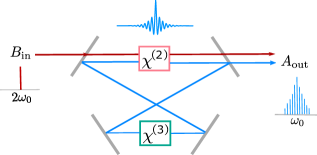
Figure 1: Schematic representation of a SR-DOPO with a Kerr nonlinear section. The cavity contains a nonlinear quadratic $(\chi^{(2)})$ medium and a section with a Kerr nonlinear one $(\chi^{(3)}).$ The cavity is driven by a continuous-wave field $B_{in}$ at frequency $2\omega_{0}$. Here only the generated signal field $A$ at frequency $\omega_{0}$ resonates, while the pump field $B$ leaves the cavity at each round-trip.

and $\varrho$, $d$ and $\eta_{2}$ are the normalized phase mismatch, group velocity mismatch or walk-off, and group velocity dispersion of the pump field, respectively [28]. This nonlocal nonlinearity acts as pump ($\mu$) depletion, and may introduce important modification on the DS dynamics and stability [35, 34]. Here, $j_{R}(k)$ mirror the dispersive two-photon absorption, while the contribution related with $j_{I}(k)$ produces a phase-shift, similar to the Kerr effect [27, 28]. In what follows, we study the formation of DSs in the absence of walk-off ($d=0$). Figure 2 shows the modification of $j_{R}(k)$ and $j_{I}(k)$ for three decreasing values of $\eta_{2}$ for $\varrho=-4$ [28].

The previous mean-field model can describe two type of systems. When $\nu_{1}=0$ and $\rho=1$, Eq. (1) models pure quadratic SR-DOPOs, where the nonlinearity is only of second order. This equation has been used to describe the formation of quadratic frequency combs [37] and DS formation in different regimes of operation [27, 28]. When $\nu_{1}\neq 0$, Eq. (1) can model a SR-DOPO with a Kerr nonlinear section like the one illustrated in Fig. 1. In that case, $\rho$ represents the ratio between the quadratic and cubic nonlinearities. This last configuration has been recently considered to study the effect of pump depletion in Kerr soliton formation [34]. Finally, when $\rho=0$ this model describes a SR-DOPO with just a Kerr section, when the pump depletion is neglected [38, 35].

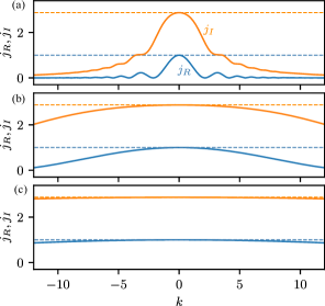
Figure 2: Modification of the kernel Fourier transform shape with $\eta_{2}$ for $(d,\varrho)=(0,-4)$. In (a) $\eta_{2}=0.5$, in (b) $\eta_{2}=0.01$, and in (c) $\eta_{2}=0.001$.The horizontal lines correspond to the values $\kappa=j_{R}(0)=1$ (blue) and $\nu_{2}=j_{I}(0)$ (orange).

III The variational formulation

Equation (1) can be derived following a variational approach [39]. This procedure requires the definition of a Lagrangian density $\mathcal{L}$ describing the conservative dynamics of the field $u$:

$$\mathcal{L}\equiv\frac{i}{2}(uu^{*}_{t}-u^{*}u_{t})-\eta_{1}u_{x}u^{*}_{x}-\frac{1}{2}\nu_{1}u^{2}u^{*2}+\delta uu^{*},$$ (5)

and a Rayleigh dissipative functional which describes the non-conservative effects [36, 40, 41, 42, 43]. In our case, the Rayleigh functional is defined as

$$\mathcal{R}=\mathcal{R}_{\alpha}+\mathcal{R}_{\mu}+\mathcal{R}_{\rho},$$ (6)

with the components

$$\mathcal{R}_{\alpha}\equiv i\alpha(uu^{*}_{t}-u^{*}u_{t}),$$ (7)

$$\mathcal{R}_{\mu}\equiv i\mu(uu_{t}-u^{*}u_{t}^{*}),$$ (8)

$$\mathcal{R}_{\rho}\equiv i\rho\left[(u^{2}\otimes J)u^{*}u_{t}^{*}-(u^{2}\otimes J)^{*}uu_{t}\right],$$ (9)

associated with losses, external driving and long-range non-local term, respectively. With these definitions, Eq. (1) can be recovered from the equation

$$i\left(\mathcal{E}+\mathcal{Q}\right)=0,$$ (10)

where $\mathcal{E}$ is the Euler-Lagrange term

$$\mathcal{E}\equiv\frac{d}{dt}\left(\frac{\partial\mathcal{L}}{\partial u^{*}_{t}}\right)+\frac{d}{dx}\left(\frac{\partial\mathcal{L}}{\partial u^{*}_{x}}\right)-\frac{\partial\mathcal{L}}{\partial u^{*}},$$ (11)

and

$$\mathcal{Q}\equiv\mathcal{Q}_{\alpha}+\mathcal{Q}_{\mu}+\mathcal{Q}_{\rho}=\frac{\partial\mathcal{R}_{\alpha}}{\partial u^{*}_{t}}+\frac{\partial\mathcal{R}_{\mu}}{\partial u^{*}_{t}}+\frac{\partial\mathcal{R}_{\rho}}{\partial u^{*}_{t}}$$ (12)

represents all the non-conservative terms. This is the general approach when dealing with dissipative systems [36, 40, 44], although there are other equivalent alternatives [45].

The parametrically forced Ginzburg-Landau approximation

Although all the variational approach previously discussed is completely general, the complexity of the nonlocal kernel $J$, makes intractable the computation of an analytical variational approximation of the DS solution. To avoid this inconvenience, in what follows, I am going to work in the broadband limit where the approximation $\mathcal{F}[J](k)\approx\mathcal{F}[J](0)$ can be considered [27]. This limit can be reached, for example, when decreasing $\eta_{2}$, as shown in Fig. 2: for $\eta_{2}=0.5$ [see Fig. 2(a)], $j_{R}$ and $j_{I}$ are quite localized in $k$ (i.e., narrowband); by decreasing $\eta_{2}$ [see Fig. 2(b) for $\eta_{2}=0.01$] $j_{R}$ and $j_{I}$ broaden; and for very small $\eta_{2}$ they are almost constant [see Fig. 2(c) for $\eta_{2}=0.001$].

As described in A, this approximation leads to,

$$\mathcal{R}_{\rho}\approx-2\rho|u|^{2}{\rm Im}\left[(\kappa+i\nu_{2})uu^{*}_{t}\right],$$ (13)

with

$$\kappa\equiv j_{R}(0)=1,\qquad\nu_{2}\equiv j_{I}(0)=\frac{{\rm sinc}(\varrho)-1}{c(\varrho)\varrho}.$$ (14)

After this consideration, Eq. (1) leads to the local parametrically forced Ginzburg-Landau equation (PFGLE)

$$u_{t}=-(\alpha+i\delta)u-i\eta_{1}u_{xx}+\mu u^{*}+\left[\rho\kappa+i(\nu_{1}+\rho\nu_{2})\right]|u|^{2}u.$$

The case with $\rho=0$, where nonlinearity reduces to a pure Kerr term , was originally proposed by Longhi [38], and utilized recently for modeling the formation of parametric Kerr DSs [35]. It is worth to mention that when temporal walk-off is very large $d\gg 1$, other kernel approximations allow the analytical integration of the convolution term as described in Ref. [34].

IV The Kantarovich optimization method: the dissipative soliton solution

This section is devoted to the derivation of a reduced effective dynamical system able to describe the main DSs features. To do so, I apply the Kantarovich method, a generalization of the Rayleigh-Ritz optimization method [36, 43, 46]. Given a parameter-dependent DS solution ansatz, this method follows a variational approach to optimize such parameters to fit the DS exact solution. Therefore, the most important part in this procedure is the election of a proper solution ansatz.

Here, based on previous works [38, 47], I propose a two-parameter DS ansatz of the form

$$u(x,t)=q_{1}(t)B[x,q_{1}(t)]e^{iq_{2}(t)},$$ (15)

with $B[x,q_{1}(t)]\equiv{\rm sech}[aq_{1}(t)x]$, where $q_{1}$ and $q_{2}$ correspond to the time-dependent amplitude and phase, respectively. The Kantarovich generalization of the Rayleigh-Ritz method consist basically in allowing these parameters depend on time. Here, the factor $a$ relates the amplitude of the soliton with its width, and to determine it, I have considered the conservative soliton formation condition as described in [48]. This condition leads to

$$a=\sqrt{\frac{\nu_{1}+\rho\nu_{2}}{2}}.$$

The temporal evolution of a DS of this form can be described using the reduced effective dynamical system derived from the Lagrangian and Rayleigh functions

$$L(q_{1},\dot{q}_{1},q_{2},\dot{q}_{2})\equiv\int_{-\infty}^{\infty}\mathcal{L}(u,u_{xx},u_{t})dx,$$ (16)

$$R(q_{1},\dot{q}_{1},q_{2},\dot{q}_{2})\equiv\int_{-\infty}^{\infty}\mathcal{R}(u,u_{t})dx.$$ (17)

After performing the integration, the effective Lagrangian becomes

$$L=\frac{2}{a}\left[q_{1}\dot{q}_{2}+\delta q_{1}-\frac{1}{3}\left(a^{2}\eta_{1}+\nu_{1}\right)q_{1}^{3}\right],$$ (18)

and the Rayleigh function reads $R=R_{\alpha}+R_{\mu}+R_{\rho},$ with

$$R_{\alpha}=\frac{4\alpha}{a}q_{1}\dot{q}_{2},$$ (19)

$$R_{\mu}=-\frac{2\mu}{a}\left[{\rm sin}(2q_{2})\dot{q}_{1}+2q_{1}{\rm cos}(2q_{2})\dot{q}_{2}\right],$$ (20)

and

$$R_{\rho}=\frac{2\rho}{a}\left(\frac{4}{3}\kappa q_{1}^{3}\dot{q}_{2}-\nu_{2}q_{1}^{2}\dot{q}_{1}\right).$$ (21)

From these functions, a 2D dynamical system, describing the evolution of $(q_{1},q_{2})$, can be derived from the dissipative version of the Euler-Lagrange equations:

$$\frac{d}{dt}\left(\frac{\partial L}{\partial\dot{q}_{j}}\right)-\frac{\partial L}{\partial q_{j}}+Q^{(j)}_{\alpha}+Q^{(j)}_{\mu}+Q^{(j)}_{\rho}=0,\qquad Q^{(j)}_{\xi}\equiv\frac{\partial R_{\xi}}{\partial\dot{q}_{j}},$$

for $j=1,2$. These equations yield the system (see derivation in C):

$$\dot{q}_{1}=-2\alpha q_{1}-\frac{4}{3}\rho\kappa q_{1}^{3}+2\mu q_{1}{\rm cos}(2q_{2}),$$ (22)

$$\dot{q}_{2}=-\delta+(a^{2}\eta_{1}+\nu_{1}-\rho\nu_{2})q_{1}^{2}-\mu{\rm sin}(2q_{2}).$$ (23)

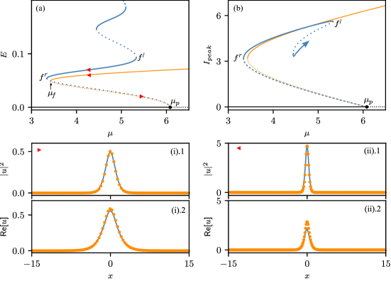
Figure 3: Comparison between numerical (blue) and analytical (orange) bifurcation diagrams and DS solutions. Panel (a) shows the DS energy as a function of $\mu$ for $\delta=-6$. Panel (b) shows the peak intensity $I_{peak}$ of the DSs shown in (a) as a function of $\mu$. Solid (dashed) lines represent stable (unstable) states. Examples of an unstable (see $\blacktriangleright$) and stable DS state (see $\blacktriangleleft$) are shown in the panels below. Here,$(\eta_{2},\varrho)=(0.01,-4)$.

The fixed points of Eqs. (22) and (22) satisfy $(\dot{q}_{1},\dot{q}_{2})=(0,0)$, and their amplitude component leads to the solutions

$$q_{1}=0,\qquad q_{1}^{(\pm)}=\pm\sqrt{\frac{\delta C_{2}-\alpha C_{1}\pm\sqrt{\Lambda}}{C_{1}^{2}+C_{2}^{2}}},$$ (24)

with

$$\Lambda\equiv(\alpha C_{1}-\delta C_{2})^{2}-(C_{1}^{2}+C_{2}^{2})(\alpha^{2}+\delta^{2}-\mu^{2}),$$ (25)

$C_{1}\equiv 2\rho\kappa/3$, and $C_{2}\equiv a^{2}\eta_{1}+\nu_{1}-\rho\nu_{2}$, as described in D. Therefore, the system has the trivial solution $q_{1}=0$, which corresponds to the continuous wave state [28], and the non-trivial solutions $q_{1}^{(+)}$, and $q_{1}^{(-)}$, which correspond to two coexisting DS states.

When these two solution meet [i.e., when $q_{1}^{(+)}=q_{1}^{(-)}$], $\Lambda=0$, and a fold bifurcation occurs at

$$q^{f}_{1}=\pm\sqrt{\frac{\delta C_{2}-\alpha C_{1}}{C_{1}^{2}+C_{2}^{2}}},$$ (26)

$$\mu_{f}^{2}=\alpha^{2}+\delta^{2}-\frac{(\alpha C_{1}-\delta C_{2})^{2}}{C_{1}^{2}+C_{2}^{2}}.$$ (27)

In contrast, if $q_{1}^{(-)}$ collides with $q_{1}=0$, a pitchfork bifurcation takes place at

$$\mu_{p}^{2}=\alpha^{2}+\delta^{2}.$$ (28)

Note that the same last expression can be obtained by means of multi-scale perturbation techniques as shown in [28].

The phase contribution to the DS solution leads to (see D):

$${\rm sin}(q_{2})=\sqrt{\frac{\mu-\alpha-2\rho\kappa q_{1}^{2}/3}{2\mu}}$$ (29)

$${\rm cos}(q_{2})=\sqrt{\frac{\mu+\alpha+2\rho\kappa q_{1}^{2}/3}{2\mu}},$$ (30)

which depends on $q_{1}$.

With all these expressions, the intensity profiles corresponding the previous DS solutions read

$$I^{(\pm)}(x)\equiv|u^{(\pm)}(x)|^{2}=[q_{1}^{(\pm)}]^{2}{\rm sech}^{2}\left(\sqrt{\frac{\nu_{1}+\rho\nu_{2}}{2}}q_{1}^{(\pm)}x\right),$$ (31)

while their real and imaginary parts are

$${\rm Re}[u^{(\pm)}(x)]=|u(x)^{(\pm)}|\sqrt{\frac{\mu+\alpha+2\rho\kappa q_{1}^{2}/3}{2\mu}},$$ (32)

$${\rm Im}[u^{(\pm)}(x)]=|u(x)^{(\pm)}|\sqrt{\frac{\mu-\alpha-2\rho\kappa q_{1}^{2}/3}{2\mu}}.$$ (33)

These expressions allow the computation of important DS magnitudes such as the peak intensity

$$I_{peak}^{(\pm)}\equiv I^{(\pm)}(0),$$ (34)

and the DS energy

$$E\equiv\int_{-\infty}^{\infty}|u^{(\pm)}(x)|^{2}dx=\frac{2\sqrt{2}q_{1}^{(\pm)}}{\sqrt{\nu_{1}+\rho\nu_{2}}}.$$ (35)

V A particular case of study: the pure quadratic SR-DOPO

To confirm the previous analytical results, I compare them with those obtained numerically in previous studies on the pure quadratic SR-DOPO scenario [28]. Thus, in what follows, I fix $\nu_{1}=0$, $\rho=1$, and $\alpha=1$. This election leads to the coefficients

$$a=\sqrt{\nu_{2}/2},\qquad C_{1}=2/3,\qquad C_{2}=(\eta_{1}-2)\nu_{2}/2.$$ (36)

Moreover, I also choose $\eta_{1}=1$, $\varrho=-4$, and $\eta_{2}=0.01$. For this regime of parameters, DSs undergo a bifurcation structure known as collapsed snaking [49] which has been characterized in detail in Ref. [28]. A portion of this curve, computed by means of path-numerical continuation methods [50], is depicted in Fig. 3(a), where the DSs energy is plotted as a function of $\mu$ for $\delta=-6$ [see blue curve]. The stability of these states has been computed numerically and is depicted using solid (dashed) lines for stable (unstable) states.

The DS states on the first stable branch, limited by the fold points $f^{l,r}$, correspond single-peak DSs with a sech-shape. The intensity and real profiles of two single-peak DSs on the stable and unstable solution branches are illustrated in Fig. 3(i), (ii) for $\mu=5.24$ and $\mu=4.27$, respectively (see blue curves). The modification of the DS peak intensity $I_{peak}$ along this diagram is also plotted in Fig. 3(b).

At this stage, there is enough information to compare these numerical results with the analytical ones obtained in Section IV. The analytical prediction of the stable and unstable DS solutions are plotted using orange dots in Figs. 3(i) and 3(ii). When regarding the intensity profiles [see Figs. 3(i).1 and 3(ii).1], the agreement is excellent. By taking a look to the real profiles, however, one can see that while the agreement is considerably good for the unstable state [see Figs. 3(i).2], it worsens for the stable one [see Figs. 3(ii).2].

The good agreement shown by the analytical prediction of the intensity seems to persist for other values of $\mu$ as depicted in Fig. 3(b) where the peak intensity of the DSs solutions [see Eq. (34)] is plotted as a function of $\mu$ using an orange line. When approaching $f^{l}$, the agreement between numerical and analytical results aggravates. With increasing $\mu$, however, the agreement is quite good for both the stable and unstable branches. Regarding the stable DSs, the variational approach does not predict the existence of the right fold $f^{r}$, and the analytical stable solution branch extends towards infinity. In contrast, for the stable states, the variational approach even describes the pitchfork point $\mu_{p}$ from where DSs arise.

It is worth to mention that, applying multi-scale perturbation theory, another approximate DS solution, complementary to the one found here, can be computed around $\mu=\mu_{p}$ [28]. This solution reads

$$u(x)=\left(\frac{\delta}{1-\mu_{p}}+i\right)\sqrt{\frac{2(\mu_{p}-\mu)}{c_{3}}}{{\rm sech}\left(\sqrt{\frac{\mu_{p}-\mu}{-c_{1}}}x\right)},$$ (37)

with

$$c_{1}\equiv\frac{-2\eta_{1}\sigma}{1+\sigma^{2}},\qquad c_{3}\equiv 2\sigma\nu_{2}(\varrho)-(\sigma^{2}-1),\qquad\sigma=\frac{\delta}{1-\mu_{p}}.$$

Figure 3(a) shows the comparison between the numerical and analytical DS energy. The analytical prediction seems to agree quite well for most of the unstable solution branch. However, as approaching the $f^{l}$, the agreement worsens.

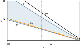
Figure 4: Phase diagram in the $(\delta,\mu)$-parameter space showing the main bifurcation lines of the system. The line with orange dots represents the analytical prediction for $f^{l}$ ($\mu_{f}$), and the black line corresponds to the pitchfork bifurcation line $\mu_{p}$. The blue shadowed area corresponds to the region of existence of DSs. Here, $(\eta_{2},\varrho)=(0.01,-4)$.

Finally, the analytical prediction for the left fold and pitchfork points, respectively Eqs. (27) and (28), permits a comparison with their numerical counterparts. Figure 4 shows the $(\delta,\mu)$-parameter plane associated with the single-peak DS states. The blue area corresponds to the region of existence of such states, and has been determined numerically by a two-parameter continuation of the left and right fold points $f^{l,r}$ shown in Fig. 3(a). The dashed vertical line in Fig. 4 corresponds to the diagrams plotted in Figs. 3(a), (b).

The position of the analytically predicted left fold [see Eq. (27)] is plotted using orange dots. This prediction works quite well for low values of $|\delta|$. However, with increasing $|\delta|$, it separates from the numerical result. In contrast, the pitchfork bifurcation line obtained using the variational approach is exactly the same one obtained applying multi-scale perturbation theory [28]. Therefore, the analytical predictions computed here can be used as good approximations for the DSs boundaries.

VI Discussion and conclusions

This work has presented an analytical study of single-peak DSs emerging in a SR-DOPO when considering two nonlinear sections: one $\chi^{(2)}$ and another $\chi^{(3)}$ . This system can be described by a generalized version of the parametrically forced Ginzburg-Landau equation which include a long-range interaction term [see Eq. (1) in Section II]. I show that equations of this type can be described using the variational formalism if non-conservative effects and the long-range interaction is taken into account through a Rayleigh dissipative functional [36]. The use of the Rayleigh functional is a standard procedure when dealing with dissipative systems, as has been shown in different contexts [36, 41, 42, 51, 52, 34].

The main result of this work is the analytical computation of an approximate single-peak DS solution in terms of the Kantarovich optimization approach (see Section IV). Starting from a suitable parameter-dependent DS solution ansatz, this approach uses the variational formalism for reducing the mean-field model to a 2D dynamical system which describes the temporal evolution of the aforementioned parameters. Thus, the fixed points of this 2D system provide a good approximation for the original DS state. Furthermore, this approach yields the analytical estimation of some DS existence boundaries, and other features, such as the DS energy and peak intensity.

The validity of these results is confirmed in Section V by comparison with the numerical bifurcation analysis performed in the context of pure $\chi^{(2)}$ SR-DOPOs [28]. The DS intensity profiles prediction and the their peak intensity match quite well the numerical results. In contrast, the agreement worsens when comparing the DSs energy. The analytical prediction of the DS boundary fold $f^{l}$ shows a quite good agreement, although it worsens a bit with increasing $|\delta|$. For the pitchfork bifurcation, however, this analysis leads to the same result than multi-scale perturbation methods [28].

The approach utilized here is very sensitive to the solution ansatz proposed. Therefore, the correct election of the ansatz is key for obtaining a good description of the solution under study. More complete ansätze, including for example temporal chirp, could lead to a better description of the system, although with a higher computational cost. In a future research, I will explore this line and seek for more accurate descriptions of the system.

Appendix A Approximation of the Kernel

In the broadband limit (see Fig. 2), we can write

$$\mathcal{F}[J](k)\approx\mathcal{F}[J](0)=\kappa+i\nu_{2},$$

where

$$\kappa\equiv\mathcal{F}[J_{R}](0)=1,\qquad\nu_{2}\equiv\mathcal{F}[J_{I}](0)=\frac{{\rm sinc}(\varrho)-1}{c(\varrho)\varrho}.$$

With this approximation, the convolution term reads

$$u^{2}\otimes J\equiv\int_{-\infty}^{\infty}u^{2}(y)J(x-y)dy\approx\qquad\qquad\qquad\qquad\qquad$$

$$\int_{-\infty}^{\infty}u^{2}(y)(\kappa+i\nu_{2})\delta(x-y)dy=(\kappa+i\nu_{2})u^{2}(x),$$

and thus, the Rayleigh functional $\mathcal{R}_{\rho}$ becomes

$$\mathcal{R}_{\rho}=i\rho\left[(u^{2}\otimes J)u^{*}u_{t}^{*}-(u^{2}\otimes J)^{*}uu_{t}\right]=\qquad\qquad\qquad$$

$$-2\rho{\rm Im}[(u^{2}\otimes J)u^{*}u_{t}^{*}]\approx-2\rho|u|^{2}{\rm Im}\left[(\kappa+i\nu_{2})uu^{*}_{t}\right].$$

Appendix B The effective Lagrangian and Rayleigh function

Inserting the ansatz defined by Eq. (15), into the Lagrangian density one obtains

$$\mathcal{L}=q_{1}^{2}\left(B^{2}\dot{q}_{2}-\eta_{1}B_{x}^{2}-\frac{\nu_{1}}{2}q_{1}^{2}B^{4}+\delta B^{2}\right),$$ (38)

which once integrated [see Eq. (16)], yields the effective Lagrangian

$$L=q_{1}^{2}\left(\dot{q}_{2}I_{a}+\delta I_{a}-\eta_{1}I_{b}-\frac{\nu_{1}}{2}q_{1}^{2}I_{c}\right)$$ (39)

with the integrals

$$I_{a}\equiv\int_{-\infty}^{\infty}B^{2}dx=\frac{2}{aq_{1}},$$

$$I_{b}\equiv\int_{-\infty}^{\infty}B_{x}^{2}dx=\frac{2aq_{1}}{3},$$

$$I_{c}\equiv\int_{-\infty}^{\infty}B^{4}dx=\frac{4}{3}\frac{1}{aq_{1}}.$$

Proceeding in a similar way with the different terms of the Rayleigh functional, the following expressions are obtained

$$\mathcal{R}_{\alpha}=-2\alpha{\rm Im}[uu^{*}_{t}]=2\alpha B^{2}q_{1}^{2}\dot{q}_{2},$$

$$\mathcal{R}_{\mu}=-2\mu\left(B^{2}q_{1}+q_{1}^{2}B\frac{\partial B}{\partial q_{1}}\right){\rm sin}(2q_{2})\dot{q}_{1}\\ -2\mu B^{2}q_{1}^{2}{\rm cos}(2q_{2})\dot{q}_{2},$$

$$\mathcal{R}_{\rho}=2\rho\left[\kappa B^{4}q_{1}^{4}\dot{q}_{2}-\nu_{2}q_{1}^{3}\left(B^{4}+q_{1}B^{3}\frac{\partial B}{\partial q_{1}}\right)\dot{q}_{1}\right].$$

After integration [see Eq. (17)], these terms leads to the Rayleigh functions

$$R_{\alpha}=2\alpha I_{a}q_{1}^{2}\dot{q}_{2},$$

$$R_{\mu}=-2\mu\left[\left(I_{a}q_{1}+q_{1}^{2}I_{d}\right){\rm sin}(2q_{2})\dot{q}_{1}+I_{a}q_{1}^{2}{\rm cos}(2q_{2})\dot{q}_{2}\right],$$

$$R_{\rho}=2\rho\left[\kappa I_{c}q_{1}^{4}\dot{q}_{2}-\nu_{2}q_{1}^{3}\left(I_{c}+q_{1}I_{e}\right)\dot{q}_{1}\right],$$

with the integrals

$$I_{d}\equiv\int_{-\infty}^{\infty}B\frac{\partial B}{\partial q_{1}}dx=-\frac{1}{aq_{1}^{2}},$$

$$I_{e}\equiv\int_{-\infty}^{\infty}B^{3}\frac{\partial B}{\partial q_{1}}dx=-\frac{1}{3aq_{1}^{2}}.$$

Appendix C The generalized Euler-Lagrange equations for the soliton parameters

In this appendix the 2D dynamical system, composed by Eqs. (22) and (23), is derived using the expressions for the effective Lagrangian and Rayleigh functions [see Eqs. (18), (19)-(21)].

For $j=1$,

$$\frac{d}{dt}\left(\frac{\partial L}{\partial\dot{q}_{1}}\right)=0,\qquad\frac{\partial L}{\partial q_{1}}=\frac{2}{a}\left[\dot{q}_{2}+\delta-(a^{2}\eta_{1}+\nu_{1})q_{1}^{2}\right],$$

$$Q^{(1)}_{\alpha}=0,\qquad Q^{(1)}_{\mu}=-\mu{\rm sin}(2q_{2})\frac{2}{a},\qquad Q^{(1)}_{\rho}=-\rho\nu_{2}q_{1}^{2}\frac{2}{a},$$

and

$$\frac{d}{dt}\left(\frac{\partial L}{\partial\dot{q}_{1}}\right)-\frac{\partial L}{\partial q_{1}}+Q^{(1)}_{\alpha}+Q^{(1)}_{\mu}+Q^{(1)}_{\rho}=0,$$

becomes

$$\dot{q}_{2}=-\delta+(a^{2}\eta_{1}+\nu_{1}-\rho\nu_{2})q_{1}^{2}-\mu{\rm sin}(2q_{2})$$ (40)

For $j=2$, a similar procedure yields

$$\frac{d}{dt}\left(\frac{\partial L}{\partial\dot{q}_{1}}\right)=\frac{2}{a}\dot{q}_{1},\qquad\frac{\partial L}{\partial q_{1}}=0,$$

$$Q^{1}_{\alpha}=\frac{4}{a}\alpha q_{1},\qquad Q^{1}_{\mu}=-\frac{4}{a}\mu q_{1}{\rm cos}(2q_{2}),\qquad Q^{1}_{\rho}=\frac{8}{3a}\rho\kappa q_{1}^{3},$$

and therefore

$$\dot{q}_{1}=-2\alpha q_{1}-\frac{4}{3}\rho\kappa q_{1}^{3}+2\mu q_{1}{\rm cos}(2q_{2})$$ (41)

Appendix D Fixed points

Here I will show the derivation of the fixed point solutions. The first fixed point condition, $\dot{q}_{1}=0$, leads to

$$q_{1}[2\alpha+\frac{4}{3}\rho\kappa q_{1}^{2}-2\mu{\rm cos}(2q_{2})]=0,$$ (42)

from where one obtains the trivial solution $q_{1}=0$ and the expression

$$\mu{\rm cos}(2q_{2})=\alpha+\frac{2}{3}\rho\kappa q_{1}^{2}$$ (43)

The condition $\dot{q}_{2}=0$ yields

$$\mu{\rm sin}(2q_{2})=-\delta+(a^{2}\eta_{1}+\nu_{1}-\rho\nu_{2})q_{1}^{2}.$$ (44)

Combining Eqs. (43) and (44), and using the condition ${\rm cos}^{2}(2q_{2})+{\rm sin}^{2}(2q_{2})=1,$ one can obtain

$$(\alpha+C_{1}q_{1}^{2})^{2}+(C_{2}q_{1}^{2}-\delta)^{2}-\mu^{2}=0,$$

and equivalently

$$(C_{1}^{2}+C_{2}^{2})q_{1}^{4}+2(\alpha C_{1}-\delta C_{2})q_{1}^{2}+\alpha^{2}+\delta^{2}-\mu^{2}=0.$$

The solutions of this bi-quadratic equation are the non-trivial solutions $q_{1}^{(\pm)}$ defined through second expression in (24).

Once $q_{1}$ is known, the contribution of the phase to the DS solutions can be obtained from Eq. (43) if one uses the equality ${\rm cos}(2q_{2})=1-2{\rm sin}(q_{2})^{2}$ and ${\rm cos}(q_{2})^{2}+{\rm sin}(q_{2})^{2}=1$. With all this, the following expressions are obtained

$${\rm sin}(q_{2})=\sqrt{\frac{\mu-\alpha-2\rho\kappa q_{1}^{2}/3}{2\mu}},$$ (45)

$${\rm cos}(q_{2})=\sqrt{\frac{\mu+\alpha+2\rho\kappa q_{1}^{2}/3}{2\mu}}.$$ (46)

References

- [1] T. Dauxois and M. Peyrard, Physics of Solitons. Cambridge University Press, Mar. 2006. Google-Books-ID: YKe1UZc_Qo8C.
- [2] N. J. Zabusky and M. D. Kruskal, “Interaction of ”solitons” in a collisionless plasma and the recurrence of initial states,” Phys. Rev. Lett., vol. 15, pp. 240–243, Aug 1965.
- [3] Y. S. Kivshar, G. P. Agrawal, and Y. S. Kivshar, Optical Solitons: From Fibers to Photonic Crystals. Mar. 2003.
- [4] B. A. Malomed, Multidimensional Solitons. AIP Publishing LLC.
- [5] N. Akhmediev and A. Ankiewicz, eds., Dissipative Solitons. Lecture Notes in Physics, Berlin Heidelberg: Springer-Verlag, 2005.
- [6] V. B. Taranenko, K. Staliunas, and C. O. Weiss, “Spatial soliton laser: Localized structures in a laser with a saturable absorber in a self-imaging resonator,” Physical Review A, vol. 56, pp. 1582–1591, Aug. 1997. Publisher: American Physical Society.
- [7] C. Weiss, M. Vaupel, K. Staliunas, G. Slekys, and V. Taranenko, “Solitons and vortices in lasers,” Applied Physics B, vol. 68, pp. 151–168, Feb. 1999.
- [8] S. Barland, J. R. Tredicce, M. Brambilla, L. A. Lugiato, S. Balle, M. Giudici, T. Maggipinto, L. Spinelli, G. Tissoni, T. Knödl, M. Miller, and R. Jäger, “Cavity solitons as pixels in semiconductor microcavities,” Nature, vol. 419, p. 699, Oct. 2002.
- [9] F. Leo, S. Coen, P. Kockaert, S.-P. Gorza, P. Emplit, and M. Haelterman, “Temporal cavity solitons in one-dimensional Kerr media as bits in an all-optical buffer,” Nature Photonics, vol. 4, pp. 471–476, July 2010.
- [10] T. Herr, V. Brasch, J. D. Jost, C. Y. Wang, N. M. Kondratiev, M. L. Gorodetsky, and T. J. Kippenberg, “Temporal solitons in optical microresonators,” Nature Photonics, vol. 8, pp. 145–152, Feb. 2014.
- [11] V. Brasch, M. Geiselmann, T. Herr, G. Lihachev, M. H. P. Pfeiffer, M. L. Gorodetsky, and T. J. Kippenberg, “Photonic chip–based optical frequency comb using soliton Cherenkov radiation,” Science, vol. 351, pp. 357–360, Jan. 2016.
- [12] K. Staliunas and V. J. Sánchez-Morcillo, “Localized structures in degenerate optical parametric oscillators,” Optics Communications, vol. 139, pp. 306–312, July 1997.
- [13] S. Longhi, “Localized structures in optical parametric oscillation,” Physica Scripta, vol. 56, pp. 611–618, Dec. 1997.
- [14] S. Trillo, M. Haelterman, and A. Sheppard, “Stable topological spatial solitons in optical parametric oscillators,” Optics Letters, vol. 22, pp. 970–972, July 1997.
- [15] K. Staliunas and V. J. Sánchez-Morcillo, “Spatial-localized structures in degenerate optical parametric oscillators,” Physical Review A, vol. 57, pp. 1454–1457, Feb. 1998.
- [16] G.-L. Oppo, A. J. Scroggie, and W. J. Firth, “From domain walls to localized structures in degenerate optical parametric oscillators,” Journal of Optics B: Quantum and Semiclassical Optics, vol. 1, pp. 133–138, Jan. 1999.
- [17] G.-L. Oppo, A. J. Scroggie, and W. J. Firth, “Characterization, dynamics and stabilization of diffractive domain walls and dark ring cavity solitons in parametric oscillators,” Physical Review E, vol. 63, May 2001.
- [18] I. Rabbiosi, A. Scroggie, and G.-L. Oppo, “A new kind of quantum structure: arrays of cavity solitons induced by quantum fluctuations,” The European Physical Journal D - Atomic, Molecular, Optical and Plasma Physics, vol. 22, pp. 453–459, Mar. 2003.
- [19] C. Etrich, U. Peschel, and F. Lederer, “Solitary Waves in Quadratically Nonlinear Resonators,” Physical Review Letters, vol. 79, pp. 2454–2457, Sept. 1997.
- [20] S. Trillo and M. Haelterman, “Excitation and bistability of self-trapped signal beams in optical parametric oscillators,” Opt. Lett., vol. 23, pp. 1514–1516, Oct 1998.
- [21] D. V. Skryabin, “Instabilities of cavity solitons in optical parametric oscillators,” Phys. Rev. E, vol. 60, pp. R3508–R3511, Oct 1999.
- [22] T. Hansson, P. Parra-Rivas, M. Bernard, F. Leo, L. Gelens, and S. Wabnitz, “Quadratic soliton combs in doubly resonant second-harmonic generation,” Optics Letters, vol. 43, pp. 6033–6036, Dec. 2018.
- [23] A. Villois, N. Kondratiev, I. Breunig, D. N. Puzyrev, and D. V. Skryabin, “Frequency combs in a microring optical parametric oscillator,” Optics Letters, vol. 44, pp. 4443–4446, Sept. 2019.
- [24] C. M. Arabí, P. Parra-Rivas, P. Parra-Rivas, T. Hansson, L. Gelens, S. Wabnitz, S. Wabnitz, S. Wabnitz, and F. Leo, “Localized structures formed through domain wall locking in cavity-enhanced second-harmonic generation,” Optics Letters, vol. 45, pp. 5856–5859, Oct. 2020.
- [25] P. Parra-Rivas, C. M. Arabí, and F. Leo, “Dark quadratic localized states and collapsed snaking in doubly resonant dispersive cavity-enhanced second-harmonic generation,” Phys. Rev. A, vol. 104, p. 063502, Dec 2021.
- [26] J. Lu, D. N. Puzyrev, V. V. Pankratov, D. V. Skryabin, F. Yang, Z. Gong, J. B. Surya, and H. X. Tang, “Two-colour dissipative solitons and breathers in microresonator second-harmonic generation,” Nature Communications, vol. 14, p. 2798, May 2023.
- [27] M. Nie and S. W. Huang, “Quadratic solitons in singly resonant degenerate optical parametric oscillators,” Phys. Rev. Appl., vol. 13, p. 044046, Apr 2020.
- [28] P. Parra-Rivas, C. Mas Arabí, and F. Leo, “Dissipative localized states and breathers in phase-mismatched singly resonant optical parametric oscillators: Bifurcation structure and stability,” Phys. Rev. Res., vol. 4, p. 013044, Jan 2022.
- [29] P. Parra-Rivas, L. Gelens, T. Hansson, S. Wabnitz, and F. Leo, “Frequency comb generation through the locking of domain walls in doubly resonant dispersive optical parametric oscillators,” Optics Letters, vol. 44, pp. 2004–2007, Apr. 2019.
- [30] P. Parra-Rivas, L. Gelens, and F. Leo, “Localized structures in dispersive and doubly resonant optical parametric oscillators,” Physical Review E, vol. 100, p. 032219, Sept. 2019.
- [31] P. Parra-Rivas, C. Mas-Arabí, and F. Leo, “Parametric localized patterns and breathers in dispersive quadratic cavities,” Physical Review A, vol. 101, p. 063817, June 2020.
- [32] M. Nie and S.-W. Huang, “Quadratic soliton mode-locked degenerate optical parametric oscillator,” Optics Letters, vol. 45, pp. 2311–2314, Apr. 2020.
- [33] A. Villois and D. V. Skryabin, “Soliton and quasi-soliton frequency combs due to second harmonic generation in microresonators,” Optics Express, vol. 27, pp. 7098–7107, Mar. 2019.
- [34] C. M. Arabí, N. Englebert, P. Parra-Rivas, S.-P. Gorza, and F. Leo, “Depletion-limited kerr solitons in singly resonant optical parametric oscillators,” Opt. Lett., vol. 48, pp. 1950–1953, Apr 2023.
- [35] N. Englebert, F. De Lucia, P. Parra-Rivas, C. M. Arabí, P.-J. Sazio, S.-P. Gorza, and F. Leo, “Parametrically driven Kerr cavity solitons,” Nature Photonics, vol. 15, pp. 857–861, Nov. 2021.
- [36] S. Chávez Cerda, S. Cavalcanti, and J. Hickmann, “A variational approach of nonlinear dissipative pulse propagation,” The European Physical Journal D - Atomic, Molecular, Optical and Plasma Physics, vol. 1, pp. 313–316, Apr. 1998.
- [37] S. Mosca, M. Parisi, I. Ricciardi, F. Leo, T. Hansson, M. Erkintalo, P. Maddaloni, P. De Natale, S. Wabnitz, and M. De Rosa, “Modulation Instability Induced Frequency Comb Generation in a Continuously Pumped Optical Parametric Oscillator,” Physical Review Letters, vol. 121, p. 093903, Aug. 2018.
- [38] S. Longhi, “Ultrashort-pulse generation in degenerate optical parametric oscillators,” Opt. Lett., vol. 20, pp. 695–697, Apr 1995.
- [39] S. Wiggins, Introduction to Applied Nonlinear Dynamical Systems and Chaos. Texts in Applied Mathematics, New York: Springer-Verlag, 2 ed., 2003.
- [40] M. Saha, S. Roy, and S. K. Varshney, “Variational approach to study soliton dynamics in a passive fiber loop resonator with coherently driven phase-modulated external field,” Phys. Rev. E, vol. 100, p. 022201, Aug 2019.
- [41] S. Roy and S. K. Bhadra, “Solving soliton perturbation problems by introducing rayleigh’s dissipation function,” Journal of Lightwave Technology, vol. 26, no. 14, pp. 2301–2322, 2008.
- [42] X. Yi, Q.-F. Yang, K. Y. Yang, and K. Vahala, “Theory and measurement of the soliton self-frequency shift and efficiency in optical microcavities,” Opt. Lett., vol. 41, pp. 3419–3422, Aug 2016.
- [43] A. Ankiewicz, N. Akhmediev, and N. Devine, “Dissipative solitons with a Lagrangian approach,” Optical Fiber Technology, vol. 13, no. 2, pp. 91–97, 2007.
- [44] A. Sahoo, S. Roy, and G. P. Agrawal, “Perturbed dissipative solitons: A variational approach,” Phys. Rev. A, vol. 96, p. 013838, Jul 2017.
- [45] I. V. Barashenkov and E. V. Zemlyanaya, “Stable complexes of parametrically driven, damped nonlinear schrödinger solitons,” Phys. Rev. Lett., vol. 83, pp. 2568–2571, Sep 1999.
- [46] D. J. Kaup and B. A. Malomed, “The variational principle for nonlinear waves in dissipative systems,” Physica D: Nonlinear Phenomena, vol. 87, no. 1, pp. 155–159, 1995.
- [47] S. Longhi, “Stable multipulse states in a nonlinear dispersive cavity with parametric gain,” Phys. Rev. E, vol. 53, pp. 5520–5522, May 1996.
- [48] G. Agrawal, Applications of Nonlinear Fiber Optics. Academic Press, Mar. 2008. Google-Books-ID: HbkKQLPE8yEC.
- [49] J. Knobloch and T. Wagenknecht, “Homoclinic snaking near a heteroclinic cycle in reversible systems,” Physica D: Nonlinear Phenomena, vol. 206, pp. 82–93, June 2005.
- [50] E. L. Allgower and K. Georg, Numerical Continuation Methods: An Introduction. Springer Series in Computational Mathematics, Berlin Heidelberg: Springer-Verlag, 1990.
- [51] H. Taheri and A. B. Matsko, “Quartic dissipative solitons in optical Kerr cavities,” Optics Letters, vol. 44, pp. 3086–3089, June 2019.
- [52] V. L. Kalashnikov and S. Wabnitz, “Stabilization of spatiotemporal dissipative solitons in multimode fiber lasers by external phase modulation,” Laser Physics Letters, vol. 19, p. 105101, Aug. 2022. Publisher: IOP Publishing.