TreeDQN: Learning to minimize Branch-and-Bound tree

Abstract

Combinatorial optimization problems require an exhaustive search to find the optimal solution. A convenient approach to solving combinatorial optimization tasks in the form of Mixed Integer Linear Programs is Branch-and-Bound. Branch-and-Bound solver splits a task into two parts dividing the domain of an integer variable, then it solves them recursively, producing a tree of nested sub-tasks. The efficiency of the solver depends on the branchning heuristic used to select a variable for splitting. In the present work, we propose a reinforcement learning method that can efficiently learn the branching heuristic. We view the variable selection task as a tree Markov Decision Process, prove that the Bellman operator adapted for the tree Markov Decision Process is contracting in mean, and propose a modified learning objective for the reinforcement learning agent. Our agent requires less training data and produces smaller trees compared to previous reinforcement learning methods.

1 Introduction

Practical applications in multiple areas such as logistics [1], portfolio management [2], manufacturing [3], and others share a combinatorial structure. Finding the optimal solution for a combinatorial task requires an exhaustive search over all valid combinations of variables. The optimal solution for a combinatorial problem formulated as a Mixed Integer Linear Program [4] can be efficiently obtained with Branch-and-Bound algorithm (B&B) [5]. B&B algorithm employs divide-and-conquer approach. At each step, it splits the domain of one of the integer variables and eliminates paths that can not lead to a feasible solution. The performance of the B&B algorithm depends on two sequential decision-making processes: variable selection and node selection. Node selection picks the next node in the B&B tree to evaluate, and variable selection chooses the next variable to split on. The variable selection process is the most computationally expensive and crucial for the performance of the whole algorithm. The optimal variable selection method, frequently dubbed as branching rule, will lead to smaller trees and a more efficient solver. Although the optimal branching rule is not known [6], all modern solvers implement human-crafted heuristics, which were designed to perform well on a wide range of tasks [7]. At the same time, practitioners frequently solve the same task with different parameters, so the branching rule adapted to a specific distribution of tasks may lead to a significant performance boost and business impact. The branching rule is applied sequentially to minimize the resulting tree size, which resembles the reinforcement learning paradigm in which an agent interacts with the environment to maximize the expected return. Recently reinforcement learning achieved state-of-the-art results in a diverse set of tasks, from beating world champions in the games of Go [8] and Dota2 [9] to aligning optical interferometer [10], controlling nuclear fusion reactor [11], tuning hyperparameters of simulated quantum annealers [12] and optimizing output of large language models [13].

Previous works [14, 15] introduced tree Markov Decision Process (tree MDP). In the tree MDP, instead of a single next state agent receives multiple next states — descendant nodes of the current tree node. The value function of the current node is the sum of reward and value functions in the child nodes. Work [14] showed that a reinforcement learning agent trained to minimize each sub-tree minimizes the whole B&B tree. We follow this approach and develop a sample efficient off-policy reinforcement learning method adapted for a tree MDP. Tree sizes produced by the B&B algorithm usually have a long-tailed distribution, even for hand-crafted branching heuristics. To overcome this challenge, we adapt the loss function to the distribution of tree sizes. As a result, our agent learns more stable, produces smaller trees, and is more sample efficient than the previous RL methods. Our contribution is the following:

1. We prove that the Bellman operator in tree MDP is contracting in mean.

2. We modify the learning objective to optimize the geometric mean.

3. We propose a novel reinforcement learning algorithm — TreeDQN.

2 Background

2.1 Mixed Integer Linear Programming

A Mixed Integer Linear Program (MILP) is a non-convex optimization problem of the form:

$$\min\Bigl{\{}c^{\top}x\colon Ax\leq b\,,x\in\bigl{[}l,u\bigr{]}\,,x\in\mathbb{Z}^{m}\times\mathbb{R}^{n-m}\Bigr{\}},$$ (1)

where objective coefficient vector $c\in\mathbb{R}^{n}$, constraint right-hand-side $b\in\mathbb{R}^{m}$, constraint matrix $A\in\mathbb{R}^{m\times n}$, lower and upper bound vectors $l,u\in\mathbb{R}^{n}$ and parameter $m\geq 1$. The method of choice to find the optimal solution of a MILP is Branch-and-Bound [5]. B&B algorithm builds a tree of nested MILP sub-problems with non-overlapping feasibility sets. The root of the tree is the original problem. At each node, B&B splits the domain of one of the integer variables into two halves, which produces two sub-problems. The sub-problems differ in their feasibility sets but share the same objective. For each sub-problem, the algorithm computes lower bound as an optimal solution for the relaxed problem with removed integrality constraints and global upper bound, which denotes the best integer feasible solution known so far. B&B uses these bounds to enforce efficiency by pruning the tree. When created, all tree nodes are as marked open. The algorithm visits every open node and either marks it as fathomed if the corresponding MILP is infeasible or the lower bound is higher than the global upper bound or splits it by an integer variable until it finds the optimal solution. Fathoming every open leaf guarantees that the B&B eventually finds the best integer-feasible solution. An example of a B&B tree is shown in Fig. 1. The resulting efficiency of the algorithm depends on the node selection strategy, which arranges the open leaves for visiting, and the branching rule, which selects an integer variable for splitting.

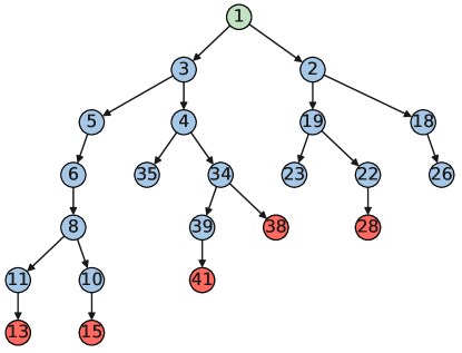
Figure 1: Branch-and-Bound tree for Combinatorial Auction task [16]. The green node is the root, blue nodes are visited, and red nodes are fathomed. Numbers indicate visiting order. Missing numbers correspond to pruned nodes.

Practical implementations of the Branch-and-Bound algorithm in SCIP [17] and CPLEX [18] solvers rely on heuristics for node selection and variable selection. Straight forward strategy for node selection is Depth-First-Search (DFS), which aims to find any integer feasible solution faster to prune branches that do not contain a better solution. In the SCIP solver, the default node selection heuristic tries to estimate the node with the lowest feasible solution. One of the best-known general heuristics for the variable selection is Strong Branching. It is a tree-size efficient and computationally expensive branching rule [19]. For each fractional variable with integrality constraint, Strong Branching computes the lower bounds for the left and right child nodes and uses them to choose the variable.

2.2 Tree MDP

The variable selection process employed by the Branch-and-Bound algorithm can be considered a tree Markov Decision Process with limitations discussed in [14, 15]. To enforce Markov property, one may either choose Depth First Search as node selection strategy [14], or set the global upper bound in the root node equal to optimal solution [15]. The state of tree MDP is the current node of the Branch-and-Bound tree, action is the fractional variable chosen for splitting, and next states are descendent nodes. The main difference between tree MDP and temporal MDP is that in tree MDP agent receives multiple next states — children nodes of the current node. Value function $V(s)$ for a tree MDP is defined as follows:

$$V^{\pi}(s_{t})=r(s_{t},a,s_{t+1}^{\pm})+V^{\pi}(s_{t+1}^{+})+V^{\pi}(s_{t+1}^{-}),$$ (2)

where $s_{t}$ is the current node of the tree, $s_{t+1}^{+}$ and $s_{t+1}^{-}$ denotes its left and right child respectively. The goal of the agent is to find a policy $\pi$ which would maximize the expected return. For instance, if the reward equals $-1$, the value function predicts the expected tree size with a negative sign. Hence, the agent maximizing the expected return would minimize the tree size.

During testing, the optimal solution for the task at hand is unknown and can not be used to set the global upper bound, which leads to a gap between training and testing environments. More efficient heuristics for node selection also induce a gap for an agent trained with DFS node selection strategy. This gap is often considered moderate and does not affect performance significantly.

3 Related work

For the first time statistical approach to learning a branching rule was applied in [20]. Authors used SVM [21] to predict the variable ranking of an expert for a single task instance. Later works [22] and [23] proposed methods based on Graph Convolutional Networks (GCNN) [24] to find an approximate solution of combinatorial tasks. In [25], authors used the same neural network architecture to imitate Strong Branching heuristic in sophisticated SCIP solver [17]. The imitation learning agent can not produce trees shorter than the expert, however, it solves the variable selection task much faster, especially if running on GPU, thereby speeding up the whole B&B algorithm significantly. In [26], authors investigate the choice of the model architecture and propose a hybrid model which combines the expressive power of GCNN with the computational efficiency of multi-layer perceptrons. Despite the time performance increase, imitation learning agents can not lead to better heuristics.

A more promising direction is to learn a variable selection rule for the Branch-and-Bound algorithm with reinforcement learning. In this approach, we will keep the guarantees of the B&B method to find an optimal solution and possibly speed up the algorithm significantly by optimal choices of branching variables. A natural minimization target for an agent in the B&B algorithm is the size of the resulting tree. One of the main challenges here is to map the variable selection process to the MDP and preserve Markov property. In the B&B search trees, the local decisions impact previously opened leaves via fathoming due to global upper-bound pruning. Thus the credit assignment in the B&B is biased upward, which renders the learned policies potentially sub-optimal. In work [14], authors propose Fitting for Minimizing the SubTree Size algorithm to learn the branching rule. In their method agent plays an episode until termination and fits the Q-function to the bootstrapped return. They used the DFS node selection strategy to enforce MDP property during training. Following this idea in work [15], authors introduce the tree MDP framework and prove that setting the global upper bound to the optimal solution for a MILP is an alternative method to enforcing MDP property. They derive policy gradient theorem for a tree MDP and evaluate REINFORCE-based agent on a set of challenging tasks similar to [25]. In both works [14] and [15], to update an agent, one needs to run an episode until the end to obtain a cumulative return. Our work improves their approaches in terms of sample efficiency and agent performance.

4 Our method

In the present work, we use an open-source implementation of the Branch-and-Bound algorithm in SCIP solver version 8.0.1. Our environment utilizes Ecole [27] 0.8.1 package, which provides an interface for learning a variable selection policy. The variable selection environment has three characteristic properties which distinguish it from an ordinary reinforcement learning environment. First of all, finding the optimal solution of a MILP is computationally demanding, which requires sample efficient learning methods. Second, the decision-making process is a tree MDP instead of a temporal MDP. Third, the distribution of tree sizes, even for the Strong Branching heuristic, has a long tail, as shown in Fig. 2.

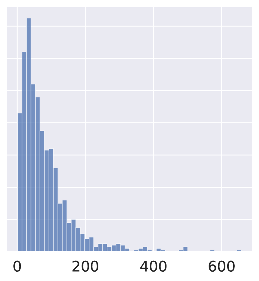
Combinatorial Auction

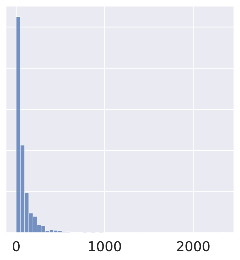
Set Cover

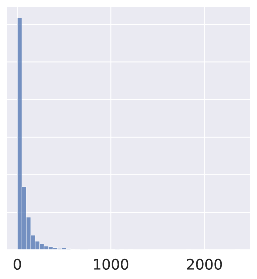
Maximum Independent Set

Figure 2: Distributions of tree sizes for Combinatorial Auction [16], Set Cover [28], and Maximum Independent Set [29] tasks, using Strong Branching heuristic for variable selection.

To reliably benchmark the average performance of different branching rules, previous works [25, 15] used the geometric mean of the final tree size as a comparison metric. This metric is more stable in the case of long-tailed distributions than the arithmetic mean. Hence, the successful reinforcement learning method should have the following properties:

1. Off-policy.

2. Work with tree MDP instead of temporal MDP.

3. Optimize geometric mean of expected return.

4.1 Contraction in mean

From the theoretical point of view, reinforcement learning methods converge to an optimal policy due to the contraction property of the Bellman operator [30]. To apply RL methods for tree MDP, we need to justify the contraction property of the tree Bellman operator.

Theorem 4.1

Tree Bellman operator is contracting in mean.

Bellman operator for a tree MDP is defined similarly to a temporal MDP:

$$T^{\pi}(V(s))=r(s,\pi(s))+\gamma\left[p_{+}V(s^{+})+p_{-}V(s^{-})\right]$$ (3)

Contraction in mean was discussed, for example, in [31]. Here, we will consider operator $T$ is contracting in mean if:

$$\|TV-TU\|_{\infty}=p\cdot\|V-U\|_{\infty},$$

$$\mathop{\mathbb{E}}p<1,$$

where the infinity norm is defined by:

$$\|V-U\|_{\infty}=\max_{s\in\mathbb{S}}|V(s)-U(s)|$$ (4)

We will assume that the probability of having a left ($p_{+}$) and a right ($p_{-}$) child does not depend on the state. This assumption is close to the B&B tree pruning process, where the pruning decision depends on the global upper bound instead of the parent node. Using the definition of tree Bellman operator (3) and the definition of the infinity norm (4) we derive the following inequality:

$$\|T^{\pi}V-T^{\pi}U\|_{\infty}=\gamma\|p_{+}V(s^{+})+p_{-}V(s^{-})-p_{+}U(s^{+})+p_{-}U(s^{-})\|_{\infty}=$$

$$\gamma\max_{s\in\mathbb{S}}\left[p_{+}|V(s^{+})-U(s^{+})|+p_{-}|V(s^{-}-U(s^{-}))|\right]\leq$$

$$\gamma(p_{+}+p_{-})\max_{x\in\mathbb{S}}|V(x)-U(x)|$$

The proof follows from the above inequality and observation that the tree is finite, i.e., $\mathop{\mathbb{E}}(p_{+}+p_{-})<1$.

4.2 Loss function

Reinforcement learning methods generally regress the expected return with the mean squared error (MSE) loss function, thereby optimizing the prediction of the arithmetic mean. In the case of vast return distributions, we propose to use mean squared logarithmic error (MSLE) instead. For a variable $y$ and targets $t_{i}$ loss $L(y,t)$ is defined as follows:

$$L(y,t)=\mathrm{MSE}(\log(|y|),\log(|t|))=\frac{1}{N}\sum_{i}(\log(|y|)-\log(|t_{i}|))^{2}$$ (5)

Since $\log(|y|)=1/N\sum\log(|t_{i}|)$ minimizes the MSE function, then the optimal value for $y$ equals to geometric mean $|y|=\exp(1/N\sum_{i=1}^{N}\log(|t_{i}|))$. Thus, the agent trained with loss (5) will be optimized to predict the geometric mean of the expected return.

In our experiments, we use Graph Convolution Neural Network with activation $f=-\exp(\cdot)$ applied for the output layer, which allows our agent to approximate a wide range of Q-values. For this activation function, we can implement the loss function (5) numerically stable using logits before activation. Hence, the proposed loss function serves two purposes simultaneously: it optimizes the target value — geometric mean of expected return and stabilizes the learning process.

4.3 TreeDQN

Our method, which we dubbed TreeDQN (1), is based on Double Dueling DQN [32] algorithm adapted for a tree MDP process (2). According to Theorem 4.1, the Bellman operator for a tree MDP process is contracting in mean. Hence, we can adapt DQN to minimize tree difference error instead of temporal difference. By sampling previous observations from experience replay, we significantly improve the sample efficiency of our method in contrast to on-policy methods [15]. We also use the loss function (5), which highly increases the learning stability.

Observation.

We use state representation in the form of a bipartite graph provided by Ecole [27]. In this graph, edges correspond to connections between constraints and variables with weight equal to the coefficient of the variable in the constraint. Each variable and constraint node is represented by a vector of 19 and 5 features, respectively.

Actions.

The agent selects one of the fractional variables for splitting. Since the number of fractional variables decreases during an episode, we apply a mask to choose only among available variables.

Rewards.

At each step, the agent receives a negative reward $r=-1$. The total cumulative return equals the resulting tree size with a negative sign.

Episode.

In each episode, the agent solves a single MILP instance. We limit the solving time for one task instance during training to $10$ minutes and terminate the episode if the time is over.

Data: Replay buffer capacity $N$, replay buffer minimum capacity $n$, discount factor $\gamma$, number of updates $t$, $\varepsilon$ decay function, batch size $b$, target update frequency $t_{up}$, random number generator R

Initialize: $Q_{\mathrm{target}}$, $Q_{\mathrm{net}}$, $\mathcal{D}\leftarrow\varnothing,\varepsilon\leftarrow 1$

Result: $Q_{\mathrm{net}}$

$s\leftarrow$ env.reset();

while $i\leq t$ do

       if R(0, 1) < $\varepsilon$ then

             a $\leftarrow$ random action;

            

      else

             a $\leftarrow\operatorname*{argmax}_{a}Q_{\mathrm{net}}(s,a)$;

            

       end if

      $s_{\mathrm{next}}$, r, $s^{+}$, $s^{-}$ = env.step(a);

       $\mathcal{D}\leftarrow\mathcal{D}\cup(s,a,r,s^{\pm})$;

       $s\leftarrow s_{\mathrm{next}}$;

       $\varepsilon\leftarrow$ decay($\varepsilon$);

       $i\leftarrow i+1$;

       if $i>n$ then

             sample batch $(s,a,r,s^{\pm})\sim\mathcal{D}$;

             $a^{\pm}\leftarrow\operatorname*{argmax}_{a^{\pm}}Q_{\mathrm{net}}(s^{\pm},a^{\pm})$;

             target = $\log\left[|r+\gamma(Q_{\mathrm{target}}(s^{+},a^{+})+Q_{\mathrm{target}}(s^{-},a^{-}))|\right]$;

             loss = $\frac{1}{b}\sum(\log(|Q_{\mathrm{net}}(s,a)|)-\mathrm{target})^{2}$;

             $Q_{\mathrm{net}}\leftarrow$ optimize($Q_{\mathrm{net}}$, loss)

       end if

      if $i\mod t_{up}$ = 0 then

             $Q_{\mathrm{target}}\leftarrow Q_{\mathrm{net}}$

       end if

      

end while

Algorithm 1 TreeDQN with experience replay

4.4 Training

In our experiments, we use a set of NP-hard tasks, namely Combinatorial Auction [16], Set Cover [28], Maximum Independent Set [29], Facility Location [33] and Multiple Knapsack [34]. To test the generalization ability of our agent, we evaluate the trained agent twice: (1) on the test instances from the training distribution and (2) on the large instances from the transfer distribution. Tab. 1 shows the parameters of the test and transfer distributions.

Table 1: Parameters used to generate train, test, and transfer tasks.

	Comb.Auct.	Set Cover	Max.Ind.Set.	Facility Loc.	Mult.Knapsack
	items / bids	rows / cols	nodes	cust. / facil.	items / knapsacks
train / test	100 / 500	400 / 750	500	35 / 35	100 / 6
transfer	200 / 1000	500 / 1000	1000	60 / 35	100 /12

We use the same set of hyperparameters (see Tab. 2) to train our agent for each task distribution. Total training time did not exceed 28 hours on an Intel Xeon 6326, NVIDIA A100 machine. To select the best checkpoint for testing, we perform validation using 30 fixed task instances every 5000 updates. The validation plot in Fig. 3 shows the geometric mean of tree sizes as a function of the number of updates. We see that during training agent learns to solve variable selection tasks better, generating smaller B&B trees.

Table 2: Agent parameters.

parameter	$\gamma$	buffer size	buffer min size	batch size	learning rate	optimizer
value	1	100’000	1’000	32	$10^{-4}$	adam

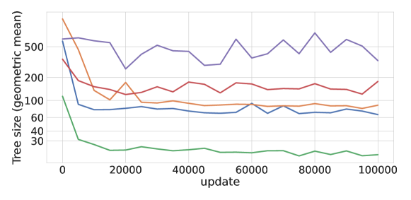
Figure 3: The geometric mean of tree size for 30 validation instances. Blue - Combinatorial Auction, orange - Set Cover, green - Maximum Independent Set, red - Facility Location, and violet - Multiple Knapsack.

5 Evaluation

In both test and transfer settings, we generate 40 task instances and evaluate our agent with five different seeds. We compare the performance of our TreeDQN agent with the Strong Branching rule, Imitation Learning agent (IL), and REINFORCE agent (tMDP+DFS, [15]). Our agent is based on the sample-efficient off-policy algorithm and requires much less training data than the REINFORCE agent. The number of episodes it took to reach the best checkpoint for TreeDQN and REINFORCE agents is shown in Tab. 3.

Table 3: Number of training episodes required to reach the best checkpoint.

Model	Comb.Auct	Set Cover	Max.Ind.Set.	Facility Loc.	Mult.Knap
TreeDQN	536	560	250	32	21
REINFORCE	22500	3000	3500	6500	9500

The evaluation results are presented in Tab. 4 and Tab. 5. We show the geometric mean of the final tree size and standard deviation computed for the same instance with different seeds and averaged over all task instances. Tab. 4 shows that the TreeDQN agent significantly exceeds the results of the REINFORCE agent in all test tasks. The TreeDQN agent is close to the Imitation Learning agent in the first four tasks and substantially outperforms the Strong Branching in the Multiple Knapsack task.

Table 4: Geometric mean with std averaged over five seeds for test tasks.

Model	Comb.Auct	Set Cover	Max.Ind.Set.	Facility Loc.	Mult.Knap
Strong Branching	48 $\pm$ 14%	43 $\pm$ 8%	40 $\pm$ 36%	294 $\pm$ 53%	700 $\pm$ 116%
IL	56 $\pm$ 12%	53 $\pm$ 9%	42 $\pm$ 32%	323 $\pm$ 46%	670 $\pm$ 120%
TreeDQN	62 $\pm$ 15%	57 $\pm$ 11%	47 $\pm$ 41%	392 $\pm$ 49%	303 $\pm$ 88%
REINFORCE	93 $\pm$ 18%	249 $\pm$ 23%	75 $\pm$ 39%	521 $\pm$ 50%	308 $\pm$ 103%

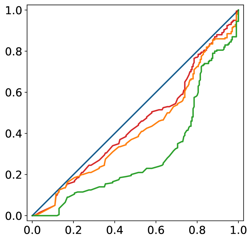
Comb.Auct.

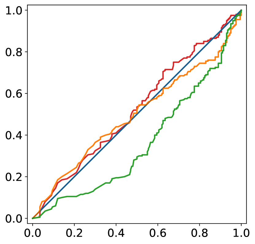
Max.Ind.Set.

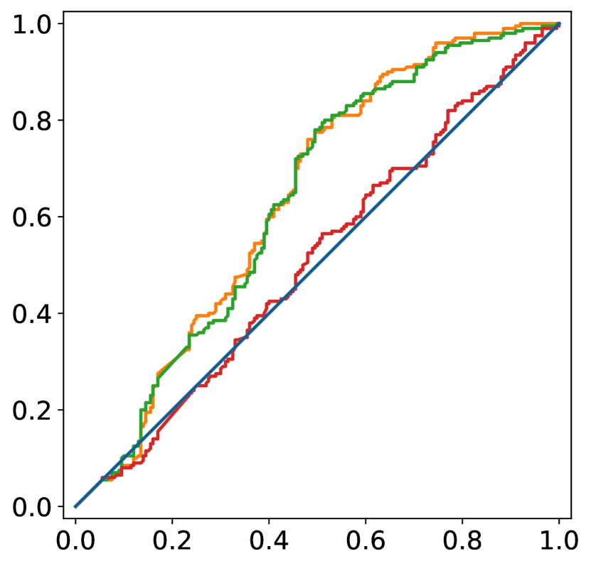
Mult.Knapsack

Figure 4: P-P plots of tree size distributions for test instances. Blue - Strong Branching, red - Imitation Learning, orange - TreeDQN, green - REINFORCE.

The geometric mean is a decent metric to compare the performance of different agents. Despite that, it loses information about the shape of the distributions. To further analyze the performance of our agent, we present distributions of tree sizes in the form of probability-probability plots (P-P plots) in Fig. 4. P-P plot allows us to compare different cumulative distribution functions (CDF). For a reference CDF $F$ and a target CDF $G$ P-P plot is constructed similar to the ROC curve: we choose a threshold $x$, move it along the domain of $F$ and draw points $(F(x),G(x))$. To show multiple distributions on the same plot, we use Strong Branching as reference CDF for all of them. If one curve is higher than another, then the corresponding CDF is larger, so the associated agent performs better. Looking at P-P plots in Fig. 4, we see that in the Combinatorial Auction task, the TreeDQN agent for all task instances performs better than the REINFORCE agent and is close to the Imitation Learning agent. In the Multiple Knapsack task, TreeDQN and REINFORCE agents outperform Strong Branching and Imitation Learning. Maximum Independent Set is a representative example. In this task, TreeDQN is good at solving simple tasks where it performs close to Imitation Learning. When the tasks become more complex, it falls behind Imitation Learning and finally behind REINFORCE. This behavior is the direct consequence of our learning objective. We optimize the geometric mean of expected tree size, so complex task instances may have less influence on the learning process. P-P plots and arithmetic means for all test tasks are shown in Appendix A, Fig. 5 and Tab. 7.

Besides testing the performance of our agent, we also study its abilities to generalize. Table 5 presents evaluation results for complex transfer tasks solved with five different seeds. Since solving complicated MILP problems is time-consuming, we limit the maximum number of nodes in a B&B tree to $200^{\prime}000$. The number of transfer tasks terminated by this node limit is shown in Appendix A, Tab. 8. It is seen from Tab. 5 that in the Set Cover, Facility Location, and Multiple Knapsack tasks, our TreeDQN agent transfers well and performs significantly better than the REINFORCE agent. In the Combinatorial Auction task both RL agents perform similarly, given the standard deviation. In the Maximum Independent Set task, the TreeDQN agent falls behind the REINFORCE agent since it adapted better for simple task instances, as seen from the P-P plot 4.

Table 5: Geometric mean with std averaged over 5 seeds for transfer tasks.

Model	Comb.Auct	Set Cover	Max.Ind.Set.	Facility Loc.	Mult.Knap
Strong Branching	665 $\pm$ 13%	122 $\pm$ 6%	845 $\pm$ 27%	722 $\pm$ 42%	57639 $\pm$ 67%
IL	867 $\pm$ 10%	149 $\pm$ 6%	2872 $\pm$ 37%	608 $\pm$ 41%	60530 $\pm$ 64%
TreeDQN	2218 $\pm$ 48%	202 $\pm$ 15%	6252 $\pm$ 42%	681 $\pm$ 38%	25701 $\pm$ 87%
REINFORCE	2171 $\pm$ 20%	858 $\pm$ 25%	1713 $\pm$ 39%	847 $\pm$ 67%	40316 $\pm$ 81%

6 Ablation study

Our modified learning objective prevents explosions of gradients and significantly stabilizes the training process. In this section, we perform an ablation study and compare the out agent with the TreeDQN agent trained with standard MSE loss. The results are shown in Tab. 6. For the majority of the tasks agent trained with a modified loss function achieves a lower geometric mean of the final tree size.

Table 6: Geometric mean with std averaged over 5 seeds for test tasks. MSE is TreeDQN agent trained with MSE loss.

Model	Comb.Auct	Set Cover	Max.Ind.Set.	Facility Loc.	Mult.Knap
TreeDQN	62 $\pm$ 15%	57 $\pm$ 11%	47 $\pm$ 41%	392 $\pm$ 49%	303 $\pm$ 88%
MSE	64 $\pm$ 17%	58 $\pm$ 10%	60 $\pm$ 50%	352 $\pm$ 49%	367 $\pm$ 110%

7 Limitations and social impact

A data-driven approach to learning a variable selection heuristic for combinatorial optimization tasks is a promising direction. High-quality heuristics will speed up combinatorial solvers significantly while keeping the guarantees to obtain the exact solution. Despite that, there are certain limitations to this approach. First, the learned heuristic depends on a concrete implementation of the Branch-and-Bound algorithm. So if the next version of the solver updates the algorithm, the heuristic will need to be retrained to prevent performance degradation. The second limitation is our learning objective. We designed our method to optimize the geometric mean of the distribution of tree sizes, so for another metric, our approach could be less efficient. The final limitation is common for all data-driven methods. If the testing task distribution is different from the training one, the performance of the whole B&B algorithm may fall dramatically.

Combinatorial optimization problems arise in multiple areas of life. A method that could compute an optimal solution faster will have a significant positive impact. However, there can be some side effects. Foremost, learning-based methods are proven to work statistically, but for a concrete task instance, they could fail. Hence, learning-based methods should be used carefully in performance-critical applications. Also, malicious users can apply combinatorial solvers to hack hashes and steal sensitive information. While current hashing algorithms seem to be hard enough, more advanced combinatorial solvers may require the development of stronger hashing algorithms.

8 Conclusion

This paper presents a novel data-efficient deep reinforcement learning method to learn a branching rule for the Branch-and-Bound algorithm. The synergy of the exact solving algorithm and data-driven heuristic takes advantage of both worlds: guarantees to compute the optimal solution and the ability to adapt to specific tasks. Our method utilizes tree MDP and contraction property of the tree Bellman operator. It maps MILP solving to an episode for our RL agent and trains the agent to optimize the final metric — the resulting size of the B&B tree. We have proposed a modified learning objective that stabilizes the learning process in the presence of high variance returns. Our approach surpasses previous RL methods at all test tasks. The code is available at https://github.com/dmitrySorokin/treedqn. In the future, we are interested in studying multitask branching agents and the limits of generalization to more complex task instances.

Appendix A Appendix

Comb.Auct.

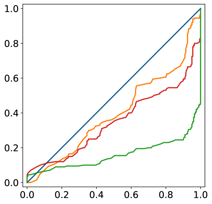
Set.Cover

Max.Ind.Set.

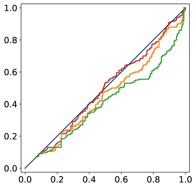
Facil.Loc.

Mult.Knapsack

Figure 5: P-P plots of tree size distributions for test instances. Blue - Strong Branching, red - Imitation Learning, orange - TreeDQN, green - REINFORCE.

Table 7: Mean with std averaged over 5 seeds for test tasks.

Model	Comb.Auct	Set Cover	Max.Ind.Set.	Facility Loc.	Mult.Knap
Strong Branching	76 $\pm$ 14%	59 $\pm$ 8%	126 $\pm$ 36%	1035 $\pm$ 53%	5139 $\pm$ 116%
IL	91 $\pm$ 14%	124 $\pm$ 8%	120 $\pm$ 34%	1113 $\pm$ 46%	4243 $\pm$ 112%
TreeDQN	104 $\pm$ 15%	80 $\pm$ 11%	528 $\pm$ 41%	1438 $\pm$ 49%	860 $\pm$ 88%
REINFORCE	160 $\pm$ 18%	722 $\pm$ 23%	210 $\pm$ 39%	2409 $\pm$ 50%	1457 $\pm$ 103%

Table 8: Number of transfer tasks finished by node limit. Total number of instances with different seeds is 200.

Model	Comb.Auct	Set Cover	Max.Ind.Set.	Facility Loc.	Mult.Knap
Strong Branching	0	0	0	10	42
IL	0	0	1	0	44
TreeDQN	2	0	13	0	13
REINFORCE	0	0	1	2	36

References

- [1] Dimitris J Bertsimas and Garrett Van Ryzin. A stochastic and dynamic vehicle routing problem in the euclidean plane. Operations Research, 39(4):601–615, 1991.
- [2] Harry Markowitz. Portfolio selection. The Journal of Finance, 7(1):77, March 1952.
- [3] Francisco Barahona, Martin Grötschel, Michael Jünger, and Gerhard Reinelt. An application of combinatorial optimization to statistical physics and circuit layout design. Operations Research, 36(3):493–513, 1988.
- [4] Laurence A Wolsey and George L Nemhauser. Integer and combinatorial optimization, volume 55. John Wiley & Sons, 1999.
- [5] Ailsa H Land and Alison G Doig. An automatic method for solving discrete programming problems. Springer, 2010.
- [6] Andrea Lodi and Giulia Zarpellon. On learning and branching: a survey. Top, 25:207–236, 2017.
- [7] Ambros Gleixner, Gregor Hendel, Gerald Gamrath, Tobias Achterberg, Michael Bastubbe, Timo Berthold, Philipp Christophel, Kati Jarck, Thorsten Koch, Jeff Linderoth, et al. Miplib 2017: data-driven compilation of the 6th mixed-integer programming library. Mathematical Programming Computation, 13(3):443–490, 2021.
- [8] David Silver, Thomas Hubert, Julian Schrittwieser, Ioannis Antonoglou, Matthew Lai, Arthur Guez, Marc Lanctot, Laurent Sifre, Dharshan Kumaran, Thore Graepel, et al. A general reinforcement learning algorithm that masters chess, shogi, and go through self-play. Science, 362(6419):1140–1144, 2018.
- [9] Christopher Berner, Greg Brockman, Brooke Chan, Vicki Cheung, Przemysław Dębiak, Christy Dennison, David Farhi, Quirin Fischer, Shariq Hashme, Chris Hesse, et al. Dota 2 with large scale deep reinforcement learning. arXiv preprint arXiv:1912.06680, 2019.
- [10] Dmitry Sorokin, Alexander Ulanov, Ekaterina Sazhina, and Alexander Lvovsky. Interferobot: aligning an optical interferometer by a reinforcement learning agent. In H. Larochelle, M. Ranzato, R. Hadsell, M.F. Balcan, and H. Lin, editors, Advances in Neural Information Processing Systems, volume 33, pages 13238–13248. Curran Associates, Inc., 2020.
- [11] Jonas Degrave, Federico Felici, Jonas Buchli, Michael Neunert, Brendan Tracey, Francesco Carpanese, Timo Ewalds, Roland Hafner, Abbas Abdolmaleki, Diego de Las Casas, et al. Magnetic control of tokamak plasmas through deep reinforcement learning. Nature, 602(7897):414–419, 2022.
- [12] Dmitrii Beloborodov, A E Ulanov, Jakob N Foerster, Shimon Whiteson, and A I Lvovsky. Reinforcement learning enhanced quantum-inspired algorithm for combinatorial optimization. Machine Learning: Science and Technology, 2(2):025009, January 2021.
- [13] OpenAI. Gpt-4 technical report. ArXiv, abs/2303.08774, 2023.
- [14] Marc Etheve, Zacharie Alès, Côme Bissuel, Olivier Juan, and Safia Kedad-Sidhoum. Reinforcement learning for variable selection in a branch and bound algorithm. In Integration of AI and OR Techniques in Constraint Programming, 2020.
- [15] Lara Scavuzzo, Feng Chen, Didier Chetelat, Maxime Gasse, Andrea Lodi, Neil Yorke-Smith, and Karen Aardal. Learning to branch with tree mdps. In S. Koyejo, S. Mohamed, A. Agarwal, D. Belgrave, K. Cho, and A. Oh, editors, Advances in Neural Information Processing Systems, volume 35, pages 18514–18526. Curran Associates, Inc., 2022.
- [16] Kevin Leyton-Brown, Mark Pearson, and Yoav Shoham. Towards a universal test suite for combinatorial auction algorithms. In Proceedings of the 2nd ACM conference on Electronic commerce. ACM, October 2000.
- [17] Ksenia Bestuzheva, Mathieu Besançon, Wei-Kun Chen, Antonia Chmiela, Tim Donkiewicz, Jasper van Doornmalen, Leon Eifler, Oliver Gaul, Gerald Gamrath, Ambros Gleixner, Leona Gottwald, Christoph Graczyk, Katrin Halbig, Alexander Hoen, Christopher Hojny, Rolf van der Hulst, Thorsten Koch, Marco Lübbecke, Stephen J. Maher, Frederic Matter, Erik Mühmer, Benjamin Müller, Marc E. Pfetsch, Daniel Rehfeldt, Steffan Schlein, Franziska Schlösser, Felipe Serrano, Yuji Shinano, Boro Sofranac, Mark Turner, Stefan Vigerske, Fabian Wegscheider, Philipp Wellner, Dieter Weninger, and Jakob Witzig. The SCIP Optimization Suite 8.0. ZIB-Report 21-41, Zuse Institute Berlin, December 2021.
- [18] IBM ILOG Cplex. V12. 1: User’s manual for cplex. International Business Machines Corporation, 46(53):157, 2009.
- [19] Tobias Achterberg. Constraint Integer Programming. July 2007. Accepted: 2015-11-20T17:32:33Z.
- [20] Elias Khalil, Pierre Le Bodic, Le Song, George Nemhauser, and Bistra Dilkina. Learning to branch in mixed integer programming. Proceedings of the AAAI Conference on Artificial Intelligence, 30(1), February 2016.
- [21] Corinna Cortes and Vladimir Vapnik. Support-vector networks. Machine learning, 20(3):273–297, 1995.
- [22] Elias Khalil, Hanjun Dai, Yuyu Zhang, Bistra Dilkina, and Le Song. Learning combinatorial optimization algorithms over graphs. In I. Guyon, U. Von Luxburg, S. Bengio, H. Wallach, R. Fergus, S. Vishwanathan, and R. Garnett, editors, Advances in Neural Information Processing Systems, volume 30. Curran Associates, Inc., 2017.
- [23] Daniel Selsam, Matthew Lamm, Benedikt Bünz, Percy Liang, Leonardo de Moura, and David L. Dill. Learning a sat solver from single-bit supervision, 2018.
- [24] Thomas N. Kipf and Max Welling. Semi-Supervised Classification with Graph Convolutional Networks. In Proceedings of the 5th International Conference on Learning Representations, ICLR ’17, 2017.
- [25] Maxime Gasse, Didier Chetelat, Nicola Ferroni, Laurent Charlin, and Andrea Lodi. Exact combinatorial optimization with graph convolutional neural networks. In H. Wallach, H. Larochelle, A. Beygelzimer, F. d'Alché-Buc, E. Fox, and R. Garnett, editors, Advances in Neural Information Processing Systems, volume 32. Curran Associates, Inc., 2019.
- [26] Prateek Gupta, Maxime Gasse, Elias Khalil, Pawan Mudigonda, Andrea Lodi, and Yoshua Bengio. Hybrid models for learning to branch. In H. Larochelle, M. Ranzato, R. Hadsell, M.F. Balcan, and H. Lin, editors, Advances in Neural Information Processing Systems, volume 33, pages 18087–18097. Curran Associates, Inc., 2020.
- [27] Antoine Prouvost, Justin Dumouchelle, Lara Scavuzzo, Maxime Gasse, Didier Chételat, and Andrea Lodi. Ecole: A gym-like library for machine learning in combinatorial optimization solvers. In Learning Meets Combinatorial Algorithms at NeurIPS2020, 2020.
- [28] Egon Balas and Andrew Ho. Set covering algorithms using cutting planes, heuristics, and subgradient optimization: A computational study, pages 37–60. Springer Berlin Heidelberg, Berlin, Heidelberg, 1980.
- [29] David Bergman, Andre A. Cire, Willem-Jan van Hoeve, and John Hooker. Decision Diagrams for Optimization. Springer International Publishing, 2016.
- [30] Tommi Jaakkola, Michael Jordan, and Satinder Singh. Convergence of stochastic iterative dynamic programming algorithms. In J. Cowan, G. Tesauro, and J. Alspector, editors, Advances in Neural Information Processing Systems, volume 6. Morgan-Kaufmann, 1993.
- [31] Alexandr A. Borovkov. Probability Theory. Springer London, 2013.
- [32] Volodymyr Mnih, Koray Kavukcuoglu, David Silver, Andrei A. Rusu, Joel Veness, Marc G. Bellemare, Alex Graves, Martin Riedmiller, Andreas K. Fidjeland, Georg Ostrovski, Stig Petersen, Charles Beattie, Amir Sadik, Ioannis Antonoglou, Helen King, Dharshan Kumaran, Daan Wierstra, Shane Legg, and Demis Hassabis. Human-level control through deep reinforcement learning. Nature, 518(7540):529–533, February 2015.
- [33] G. Cornuejols, R. Sridharan, and J.M. Thizy. A comparison of heuristics and relaxations for the capacitated plant location problem. European Journal of Operational Research, 50(3):280–297, feb 1991.
- [34] Alex S. Fukunaga. A branch-and-bound algorithm for hard multiple knapsack problems. Annals of Operations Research, 184(1):97–119, November 2009.