An Accelerated Stochastic ADMM for
Nonconvex and Nonsmooth Finite-Sum Optimization
Yuxuan Zeng,
Zhiguo Wang,
Jianchao Bai, and Xiaojing Shen
Yuxuan Zeng, Zhiguo Wang (corresponding author), and Xiaojing Shen are with College of Mathematics, Sichuan University, 610064, Chengdu, China (e-mail: 2020222010085@stu.scu.edu.cn, wangzhiguo@scu.edu.cn, shenxj@scu.edu.cn).Jianchao Bai (corresponding author) is with Research & Development Institute of Northwestern Polytechnical University in Shenzhen, Shenzhen 518057, China; School of Mathematics and Statistics, Northwestern Polytechnical
University, Xi’an 710129, China (e-mail: jianchaobai@nwpu.edu.cn).
Abstract
The nonconvex and nonsmooth finite-sum optimization problem with linear constraint has attracted much attention in the fields of artificial intelligence, computer, and mathematics, due to its wide applications in machine learning and the lack of efficient algorithms with convincing convergence theories.
A popular approach to solve it is the stochastic Alternating Direction Method of Multipliers (ADMM), but most stochastic ADMM-type methods focus on convex models. In addition, the variance reduction (VR) and acceleration techniques are useful tools in the development of stochastic methods due to their simplicity and practicability in providing acceleration characteristics of various machine learning models. However, it remains unclear whether accelerated SVRG-ADMM algorithm (ASVRG-ADMM), which extends SVRG-ADMM by incorporating momentum techniques, exhibits a comparable acceleration characteristic or convergence rate in the nonconvex setting.
To fill this gap, we consider a general nonconvex nonsmooth optimization problem and study the convergence of ASVRG-ADMM.
By utilizing a well-defined potential energy function, we establish its sublinear convergence rate , where denotes the iteration number.
Furthermore, under the additional Kurdyka-Lojasiewicz (KL) property which is less stringent than the frequently used conditions for showcasing linear convergence rates, such as strong convexity, we show that the ASVRG-ADMM sequence almost surely has a finite length and converges to a stationary solution with a linear convergence rate. Several experiments on solving the graph-guided fused lasso problem and regularized logistic regression problem validate that the proposed ASVRG-ADMM performs better than the state-of-the-art methods.
Keywords Nonconvex and nonsmooth optimization, acceleration techinque, stochastic ADMM, convergence.
I Introduction
In recent years, machine learning has been studied and applied extensively in system identification [1], and automatic control [2].
In this paper, we consider a class of the nonconvex nonsmooth finite-sum optimization problems with a linear constraint in machine learning, as follows:
(1)
where consists of the summation of components, i.e., and is assumed smooth, but can be nonconvex; is convex but possibly nonsmooth; the constraint is used for encoding the structure pattern of model
parameters, where , , . To motivate our work, we first briefly discuss one common setting related to problem (1).
Let us consider a binary classification task. Specifically, given a set of training samples , , where is the input data and its corresponding label is . Then we use the famous graph-guided fused Lasso model [3] to learn the parameter, which can be represented as
(2)
where the sigmoid loss function is as defined by , which is a nonconvex function. is a given matrix decoded the sparsity pattern of the graph, which is obtained by sparse inverse covariance matrix estimation [4]. In order to solve (2), we can introduce an additional primal variable , and
reformulate the problem (2) as a special case of (1)
where and .
The problem (1) also attracts attention and arises in many other fields such as statistical learning [5], computer vision [6] and 3D CT image reconstruction [7].
In the following text, we focus on the composite finite-sum equality-constrained optimization problem (1) and check the efficiency of this paper from both algorithmic and theoretical perspectives.
I-ARelated work
One of the popular methods to solve the general optimization (1) is ADMM algorithm [8, 9, 10]. Specifically, at the -th iteration, the typical sequential update steps are
(3)
where is the dual variable and
(4)
is an augmented Lagrangian (AL) function and is a penalty parameter.
Many ADMM-type algorithms, such as proximal ADMM [11, 9, 12], inexact ADMM [8, 13], linearized/relaxed ADMM [14, 15], and consensus ADMM [16, 17] have been proposed to solve the subproblem in (3) efficiently. Recently,
a proximal AL method with an exponential averaging scheme was proposed by [18] to
handle nonconvex optimizations.
Large-scale optimization problems (1) typically involve a large sum of component functions, making it infeasible for deterministic ADMMs to compute the full gradient on all training samples at each iteration.
Stochastic gradient descent (SGD) has a much lower per-iteration complexity than deterministic methods by utilizing only one sample’s gradient at each iteration.
Stochastic ADMM (SADMM), proposed in [19], combines SGD and ADMM, and the update step of variable in SADMM is approximated as follows:
(5)
where we selet the random variable uniformly at random from , is the step-size, and with given positive semi-definite matrix .
However, when the objective function is convex, stochastic ADMMs have been proved to own the worst-case convergence rate, which is lower than the deterministic ADMMs with convergence rate.
The gap in convergence caused by the high variances of stochastic gradients can be tackled by combining stochastic variance reduction gradient (SVRG) methods [20] with ADMM, resulting in the SVRG-ADMM in [21]. Unlike SADMM, variance-reduced ADMM aims to find an unbiased gradient estimator whose variance will vanish as the algorithm converges.
This encourages the selection of a larger step-size, such as a constant step-size , to improve the convergence rate.
Specifically, we compute the gradient for each iteration as follows:
(6)
where is defined in the equation (5), and is an unbiased estimator of the gradient , i.e., .
The Nesterov acceleration technique [22] enjoys a fast convergence rate and has been successfully applied to train many large-scale machine learning models, including deep network models. Directly extending the Nesterov acceleration technique to the stochastic settings may aggravate the inaccuracy of the stochastic gradient and harm the convergence performance. [13] proposed ASVRG-ADMM, an accelerated SVRG-ADMM method by introducing a new Katyusha momentum acceleration trick [23] into SVRG-ADMM. Table I presents a comparison of several stochastic ADMM algorithms. All algorithms in the table incorporate the VR technique, while only the last three employ momentum acceleration techniques.
Although ASVRG-ADMM has been successful in convex problems, its behavior in nonconvex nonsmooth problems remains largely unknown.
Many important applications, such as signal/image processing [24], computer vision [6], and video surveillance [25], involve nonconvex objective functions that are beyond the scope of the theoretical conditions under which ASVRG-ADMM [13] has been proven to converge.
Therefore, there exists a gap in the theoretical convergence analysis between extant ASVRG-ADMM in the convex scenario and ASVRG-ADMM in the nonconvex scenario.
To fill this gap, this paper addresses two crucial problems:
Q1.
Whether the ASVRG-ADMM algorithm can converge to the stationary point for the common nonconvex nonsmooth finite-sum optimization?
Q2.
If the algorithm converges, can we establish its linear convergence rate such as R-linear111
The sequence converges to R-linearly if
for all , and the sequence converges to zero Q-linearly.
Then one can always find a suitable sequence
as , such that
for all , where .
convergence?
TABLE I: Comparison of convergence rates of some stochastic ADMM algorithms.
In this paper, we develop ASVRG-ADMM for the nonconvex and nonsmooth problems (1). ASVRG-ADMM is inspired by the momentum [13, 8, 23] and the variance reduction [20, 21] technique. In addition, it has several new features. First, compared with [13], we consider the nonconvex objective function rather than the convex function, which poses a major obstacle to establishing the convergence of our algorithm without
the sufficiently decreasing property of the AL function.
Second, compared with SVRG-ADMM in [21],
our proposed algorithm employs the Katyusha momentum technique to improve the accuracy of the stochastic gradient and facilitate faster convergence in practice.
In summary, our main contributions include four folds as follows:
(C1)
We propose a novel accelerated stochastic ADMM (ASVRG-ADMM) for the nonconvex and nonsmooth problem (1), which enjoys the advantages of both the momentum acceleration technique [23, 13] and the variance reduction technique [21, 20].
(C2)
By introducing a potential energy function related to the AL function of (1), we establish the sublinear convergence rate , then we answer Q1.
While ASVRG-ADMM has the same convergence rate as SVRG-ADMM [21], theoretically, we can achieve faster decay of the potential energy function than SVRG-ADMM by selecting the optimal momentum parameter. Furthermore, our algorithm achieves better convergence in numerical experiments.
(C3)
We establish the almost sure R-linear convergence rate of ASVRG-ADMM by utilizing the extra KL property to answer Q2, as listed in Table I
and demonstrated in Theorem 2.
Answering Q2 under the nonconvex and nonsmooth setting is not a trivial task due to the inclusion of both the momentum term and variance reduction technique.
To the best of our knowledge, this is the first almost sure linear convergence result for the accelerated stochastic ADMM algorithm with variance reduction technique.
Various numerical experiments demonstrate the effectiveness of our ASVRG-ADMM, as it exhibits both lower variance and faster convergence compared to several advanced stochastic ADMM-type methods [21, 19].
Synopsis: The remainder of this paper is organized as follows. Section II introduces the notations and mild assumptions. We present the framework of ASVRG-ADMM in
Section III. We
study its convergence
and extends the theoretical analysis of the almost sure linear convergence rate under the extra KL property in Section IV. Section V presents some numerical results to demonstrate the effectiveness and efficiency of the method. Finally, we conclude the paper with discussions.
Notation: The symbol denotes the Euclidean norm of
a vector (or the spectral norm of a matrix), and is
the -norm, i.e., . We use
, and to denote the sets of real numbers, dimensional real column vectors, and real matrices, respectively.
Let be the probability space, be a random variable, denote the expectation,
denote the conditional expectation of given sub--algebra , and employ the abbreviations “a.s.” for “almost surely”. Let denote the identity matrix and denote the zero matrix.
We denote by the gradient of if it is differentiable, or any of the subgradients of the function .
Let and be the smallest and largest eigenvalues of matrix , respectively;
and let and denote the smallest and largest eigenvalues of positive matrix , respectively.
For a nonempty closed set denotes the distance from to set .
II Preliminaries
II-ABasic Assumptions and Definitions
Before establishing the convergence analysis, we clarify the following proper assumptions.
Assumption 1
For , each function possesses a
Lipschitz continuous gradient with the constant , that is
where .
Assumption 2
and are lower bounded.
Assumption 3(feasibility)
, where returns the image of a matrix.
Assumption 4(Lipschitz sub-minimization paths)
For any fixed has a unique minimizer. In addition, defined by is a Lipschitz continuous map.
Assumption 1 is a standard smoothness assumption. Note that Assumptions 1-2 are satisfied for the case of , . Assumptions 3-4 are proposed in [27], which weaken the full column rank assumption typically imposed on matrices and .
Moreover, Assumptions 3-4 are the mild assumptions commonly used to ensure that the dual variable is controlled by the primal variable, see Lemma 1.
Next, we introduce the critical point and KL property used in this paper.
Definition 1
The point is denoted as the feasible solution set of the problem (1).
When there exist a optimal point and a dual variable for the problem (4), the KKT conditions are satisfied as follows:
We also say that satisfy the KKT conditions is exactly a critical point of the AL function, denoted as .
A proper lower semicontinuous function is said to possess the KL property at dom if there exist a constant , a neighborhood of and a continuous concave function , satisfying the following requirements:
•
, and for all ;
•
for all , the KL inequality holds:
(7)
Many effective functions satisfy the KL property, including but not limited to , , log-exp, and the logistic loss function . For more examples, readers can refer to [28, 29], [30, 31], and [32](see Page 919).
Therefore, the potential energy function defined in (15) can easily satisfy the KL property.
Remark 1
When function in Definition 2 is differentiable, then the KL property becomes the PL property [33], which is much weaker than the strongly convex property, and widely used to show the global convergence in the field of deep learning. However, the PL property only deals with smooth differentiable functions. In this paper, the considered problem (1) not only has the smooth term but also has the nonsmooth term, thus we use the KL property to show the linear convergence.
III Developments of ASVRG-ADMM
We propose ASVRG-ADMM, which incorporates momentum and variance reduction techniques to ensure fast convergence of the nonsmooth and nonconvex problem (1). The algorithm, presented in Algorithm 1, consists of epochs, each containing iterations with typically chosen to be .
Input:parameter and initial values of , , and .
Output:Iterate and chosen from .
fordo
, and ;
;
fordo
Uniformly and randomly choose a random variable from , and compute in (6) ;
The first step is to update the primal variable in (8) by solving
(12)
If , one can observe that the optimization (12) has closed form solution with
where is the regularization parameter.
III-BUpdate of Auxiliary Variable
Inspired by Katyusha [23, 13] acceleration tricks, the second step is adopting an auxiliary variable before updating the primal variable .
A surrogate function is first introduced to approximate the objective function in (3) and the update rule of is formulated as follows:
(13)
where is the learning rate or step-size, and is the stochastic variance reduced gradient
estimator defined in (6).
In general, the direct solution of (13) can be challenging or even infeasible since it requires the inversion of .
To alleviate this computational burden, the inexact Uzawa method can be employed to linearize the last term (13).
Specifically, we can select with to ensure that , which results in the simpler closed-form solution of (13) as (9).
III-CMomentum Accelerated Update Rule for
The next step is our momentum accelerated update rule for the primal variable , as given below:
(14)
where is a momentum parameter, and is a momentum term,
which uses the final output iterate from the previous epoch (updated every m iterations in the inner loop), i.e., , to speed up our algorithm.
In (14), we leverage the Katyusha momentum technique [23], which uses a convex combination of the latest and snapshot ,
whereas the Nesterov-type momentum technique uses a nonconvex extrapolation of the two latest iterates.
Compared with Nesterov momentum, Katyusha momentum ensures that
the iterates do not deviate too far from , which ensures accurate gradient estimation.
III-DUpdate of Dual Variable
The final step is to update the dual variable by
Note that we use auxiliary variable rather than the primal variable [19] in the dual update scheme, which helps us to establish the convergence of the proposed algorithm under nonconvex setting.
Before ending the section, let’s make a few remarks about ASVRG-ADMM.
Remark 2
Compared with SVRG-ADMM [21], our ASVRG-ADMM incorporates a new acceleration step (14) and its sublinear and linear convergence have been established under weaker Assumption 3- 4. Additionally, if we set in the update step of to 1, it results in the algorithm degenerating into SVRG-ADMM [21], where , which can be evidenced by the overlapping descent curves of ASVRG-ADMM1 () and SVRG-ADMM in Figure 3 (left).
IV Convergence Analysis
This section establishes the sublinear and linear convergence of our proposed ASVRG-ADMM for nonconvex and nonsmooth problems.
In the literature, the AL function [27] is frequently used as the potential energy function with sufficiently decreasing property (see [27]). However, in the nonconvex setting, our Algorithm 1 deviates from this approach.
To ensure sufficient decrease and convergence, we present the following lemmas and theorems with a practical sequence of potential energy functions defined as follows:
(15)
where the positive sequence and the parameter will be decided in the following Lemma 2.
Let be a stochastic process adapted to the filtration , where , is the -field, and we abbreviate
as , see more details in [7, 30]. Additionally, we define as .
Now, we first provide an outline of the proof in this section.
•
Firstly, we propose a new potential energy function, which differs from the one in [21], and prove the monotonicity of this function.
•
Next, we leverage the monotonicity property of the potential energy function to establish the convergence rate of the newly defined sequence in (24).
•
Lastly, we leverage the KL property along with finite-length property in Lemma 3 to achieve a almost sure linear convergence result for ASVRG-ADMM.
Our convergence analysis will utilize a bound on the term , which is given by Lemma 1.
Lemma 1(Upper bound of )
Given Assumptions 1-3, for generated by the Algorithm 1,
we can have the following result
For the sequence generated by Algorithm 1, assuming that Assumptions 1-3 hold, and the positive sequences and exist, we choose positive parameters , , , , , , and such that
then the sequence is sufficiently decreasing:
(17)
Proof 2
The specific expression of the tuple and the sequences , are provided in Appendix B.
Remark 3
As we see, there are some crucial parameters in Lemma 2. In this remark, we further clarify how to choose these parameters . One can observe that there exists a parameter in the right side of the inequality (17). If promotes larger, then the sequence decreases faster.
•
Firstly, we rewritten defined in (S.5) as follows:
(18)
where
(19)
(20)
•
Secondly, in order to obtain the maximum value of , then the optimal parameters and can be obtained
(21)
(22)
•
Finally, from (21) and (22), we can see that the optimal and become larger, the parameter should be adjusted to smaller.
Remark 4
Now we show that there also exit a lower bound for the dual step size .
Taking the optimal value of in (22) into in (18), we study the requirement of with the inequality , which is simplified as follows:
Considering the setting of , the parameter should satisfy the following inequality
which indicates
(23)
Based on the above important descending Lemma 2, we next
analyze the convergence and iteration complexity of the ASVRG-ADMM with the aid of a simple notation:
(24)
We also denote
Theorem 1
Assuming that Assumptions 1-3 hold, let be the sequence generated by Algorithm 1, using the identical notations as in Lemma 2. For , where and , the following can be derived:
Theorem 1 shows that Algorithm 1 converges with the worst-case convergence rate, where .
Lemma 3(The Finite Length Property)
Let the sequence be generated by Algorithm 1 under Assumptions 1-4 and has the KL property at the stationary point with
KL exponent (see the Definition 2). Suppose that
and are semi-algebraic functions satisfying the KL inequality, then has a finite length, that is,
Now, combined with the KL property defined in Definition 2 (see [28]), we can obtain the linear convergence rate of ASVRG-ADMM.
Theorem 2(Linear Convergence)
For notational simplicity, we also omit the upper script . The sequence is generated by Algorithm 1, and it converges to . Additionally, we define . Assume that defined in (15) has the KL property at the stationary point with an exponent . Then, we draw the following estimations under Assumptions 1-4:
i)
If , then the sequence converges a.s. in a finite number of steps.
ii)
If , then there exists and , such that
iii)
If , then there exists , such that
Proof 5
We also give a sketch of the proof and refer to Appendix G for more details. This proof is structured by two main steps which contain:
•
First, we define a new sequence and prove it converges a.s. to zero Q-linearly.
•
Second, we conclude that the sequence is bounded by the newly defined sequence which converges a.s. Q-linearly, thus the sequence converges a.s. to R-linearly.
Remark 5
We prove in Theorem 2 that our ASVRG-ADMM almost surely achieves R-linear convergence at the rate of for nonconvex nonsmooth optimization, in accordance with the definition of R-linear convergence presented in Section I.
We construct a potential energy function in (15) that satisfies the KL property to ensure convergence when . This is the first demonstration of linear convergence for a stochastic ADMM incorporating momentum and variance reduction techniques.
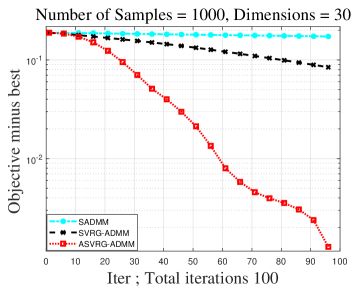
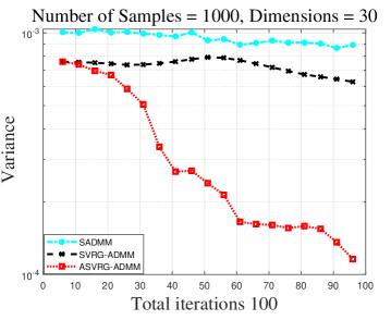
Figure 1: Comparison of the SADMM, SVRG-ADMM, and
ASVRG-ADMM algorithms for the nonconvex quadratic problem in the synthetic setting. The objective values (left) and variances of gradient (right).
V Numerical Experiments
In this section, we examine the numerical performance of the proposed ASVRG-ADMM algorithm
and present comparison results with the existing methods.
We conducted several different real dataset experiments to validate our theoretical results and show the high efficiency of the implementation of our proposed ASVRG-ADMM algorithmic framework.
We compare ASVRG-ADMM with the following
state-of-the-art methods for nonconvex problems: SADMM in [19], SVRG-ADMM in [21], and SAG-ADMM in [21]. In the following, all algorithms were
implemented in MATLAB, and the experiments were performed on a PC with an Intel i7-12700F CPU and 16GB memory.
V-ASynthetic Data For the Nonconvex Quadratic Problem
Our setup for the synthetic nonconvex quadratic problem is as follows. We first generate the symmetric matrix from the standard Gaussian distribution. Next, the matrix or , where is obtained from a sparse inverse
covariance estimation given in [3]. Then we solve the following nonconvex quadratic problem:
where is a positive regularization parameter. Finally, all experimental results are averaged over 300 Monte Carlo experiments.
From Fig.1, we can see the training loss (i.e., the training objective value minus the best value) and the variance
of SADMM [19], SVRG-ADMM [21], and ASVRG-ADMM for the nonconvex quadratic problem. All the experimental results show that our ASVRG-ADMM method with smaller variance converges consistently much faster than both SADMM and SVRG-ADMM, which empirically verifies our theoretical results of the effectiveness of the momentum technique resulting in faster convergence.
V-BGraph-Guided Fused Lasso
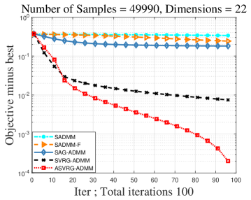
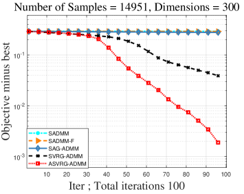
Figure 2: Comparison of different stochastic ADMM methods
for graph-guided fused lasso problems on the two
data sets: ijcnn1 (left) and w8a (right).
We first evaluate the proposed method for solving the graph-guided fused Lasso problem (2). We set , , and , similar to [21].
Two cases are taken into account in Algorithm 1, particularly: a time-varying stepsize parameter
for the SADMM; a fixed parameter for the SADMM-F.
The parameter has been set for the SVRG-ADMM algorithm. At last, the result of all experiments is averaged over 30 Monte Carlos experiments.
We use real datasets ijcnn1, a9a, and w8a downloaded from LIBSVM
to test our proposed method.
The training error of all the methods is shown in Fig.2.
The results indicate that
compared to algorithms without variance reduction techniques, e.g., SADMM and SADMM-F, the variance reduced stochastic ADMM algorithms (including both SVRG-ADMM and ASVRG-ADMM) converge substantially more quickly.
Notably, in terms of the experimental convergence performance, ASVRG-ADMM consistently outperforms all comparison algorithms under all datasets, which is consistent with our theoretical analysis.
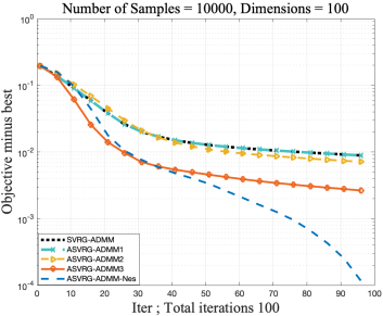
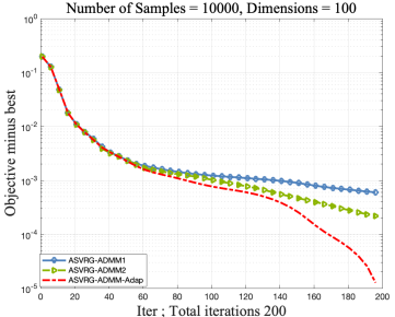
Figure 3:
Comparison of ASVRG-ADMM algorithm for different (left) and (right) on Graph-Guided Fused Lasso using synthetic data.
We compare various values of momentum in Figure 3, namely the larger value (ASVRG-ADMM2), the smaller but empirically superior value (ASVRG-ADMM3), and the Nesterov-type momentum parameter [22, 13] (ASVRG-ADMM-Nes).
The results indicate that smaller values of lead to improved experimental outcomes while employing the Nesterov-type decaying momentum parameter results in optimal performance.
Furthermore, we conduct additional comparisons using different values of as shown in Figure 3.
The value of in ASVRG-ADMM1 exceeded the experimentally optimal value of in ASVRG-ADMM2.
To satisfy the lower bound inequality (23), an adaptive approach known as ASVRG-ADMM-Adap [34] can be employed. This approach gradually increases by setting , where , to ensure the validity of (23). Smaller values of yield improved experimental performance, with the adaptive approach achieving the best results.
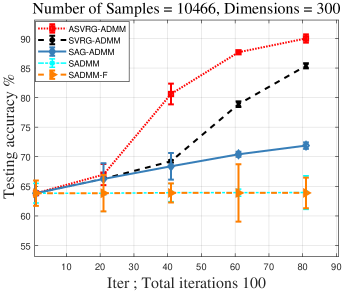
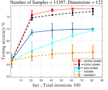
V-CRegularized Logistic Regression
In this subsection, we evaluate the test data performance of ASVRG-ADMM for solving the nonconvex Regularized Logistic Regression (RLR) problem
where is defined the same as in (2), and the parameter . In addition, we randomly select 60% of the data to train the models and the rest to test the performance.
Fig.4 shows the experimental results of datasets w8a (left) and a9a (right) respectively. Fig.4 indicates that both the algorithm SADMM and SADMM-F consistently converge more slowly than the others and the variances of these two algorithms are larger than the others in all settings, which empirically verifies that variance reduced stochastic ADMM algorithms with smaller variance can perform better. We observe that SVRG-ADMM and ASVRG-ADMM consistently outperform the others. Moreover, ASVRG-ADMM performs much better than the other methods in all settings, which again verifies the effectiveness of our
ASVRG-ADMM method with the accelerated momentum technique.
Figure 4: Comparison of different stochastic ADMM methods
for the accuracy of logistic regression problems.
VI Conclusion and Future Work
In this paper,
we integrated both momentum acceleration and the variance reduction trick into stochastic ADMM and proposed an efficient accelerated stochastic variance reduced ADMM for solving the common nonconvex nonsmooth problems.
Furthermore, we theoretically
proved that ASVRG-ADMM obtains a similar convergence to SVRG-ADMM [21] for nonconvex problems. Especially under the KL property, the convergence rate of ASVRG-ADMM can be improved to the almost sure linear convergence rate. Compared to those of the state-of-the-art stochastic ADMM methods such as SVRG-ADMM, massive experimental results validate the numerical advantages of our proposed algorithm.
For future work, there are some interesting directions such as the research of applying the momentum acceleration trick to other
algorithms like SAG-ADMM and
SAGA-ADMM [21], and the research of the theoretical improvement of the convergence rate of the proposed method.
In addition, it is also interesting to extend ASVRG-ADMM and theoretical results to the distributed optimization and nonsmooth and nonconvex optimization.
References
[1]
G. Pillonetto, F. Dinuzzo, T. Chen, G. De Nicolao, and L. Ljung, “Kernel
methods in system identification, machine learning and function estimation: A
survey,” Automatica, vol. 50, no. 3, pp. 657–682, 2014.
[2]
L. Li, H. Luo, S. X. Ding, Y. Yang, and K. Peng, “Performance-based fault
detection and fault-tolerant control for automatic control systems,”
Automatica, vol. 99, pp. 308–316, 2019.
[3]
S. Kim, K.-A. Sohn, and E. P. Xing, “A multivariate regression approach to
association analysis of a quantitative trait network,”
Bioinformatics, vol. 25, no. 12, pp. i204–i212, 2009.
[4]
J. Friedman, H. Trevor, and R. Tibshirani, “Sparse inverse covariance
estimation with the graphical lasso,” Biostatistics, vol. 9, no. 3,
pp. 432–441, 2008.
[5]
J. Bai, H. Zhang, and J. Li, “A parameterized proximal point algorithm for
separable convex optimization,” Optimization Letters, vol. 12,
no. 7, pp. 1589–1608, 2018.
[6]
N. P. Papanikolopoulos and P. K. Khosla, “Adaptive robotic visual tracking:
Theory and experiments,” IEEE Transactions on Automatic Control,
vol. 38, no. 3, pp. 429–445, 1993.
[7]
F. Bian, J. Liang, and X. Zhang, “A stochastic alternating direction method
of multipliers for non-smooth and non-convex optimization,” Inverse
Problems, vol. 37, p. 075009, 2021.
[8]
J. Bai, W. Hager, and H. Zhang, “ An inexact accelerated stochastic ADMM for
separable convex optimization,” Computational Optimization and
Applications, vol. 81, no. 2, pp. 479–518, 2022.
[9]
Y. Yang, Q. Jia, and e. a. Xu, Zhanbo, “Proximal ADMM for nonconvex and
nonsmooth optimization,” Automatica, vol. 146, p. 110551, 2022.
[10]
M. Chao, D. Han, and X. Cai, “Convergence of the peaceman–rachford splitting
method for a class of nonconvex programs,” Numerical Mathematics:
Theory, Methods and Applications, vol. 14, no. 2, pp. 438–460, 2021.
[11]
K. Guo, D. Han, and T. Wu, “ Convergence of ADMM for optimization problems
with nonseparable nonconvex objective and linear constraints,”
Pacific Journal of Optimization, vol. 14, pp. 489–506, 2018.
[12]
Z. Wu and M. Li, “General inertial proximal gradient method for a class of
nonconvex nonsmooth optimization problems,” Computational Optimization
and Applications, vol. 73, pp. 129–158, 2019.
[13]
Y. Liu, F. Shang, H. Liu, L. Kong, L. Jiao, and Z. Lin, “ Accelerated
variance reduction stochastic ADMM for large-scale machine learning,”
IEEE Transactions on Pattern Analysis and Machine Intelligence,
vol. 43, no. 12, pp. 4242–4255, 2020.
[14]
J. Bai, D. Han, H. Sun, and H. Zhang, “Convergence on a symmetric accelerated
stochastic ADMM with larger stepsizes,” CSIAM Transactions on Applied
Mathematics, vol. 31, no. 3, pp. 448–479, 2022.
[15]
M. Tao, “Convergence study of indefinite proximal ADMM with a relaxation
factor,” Computational Optimization and Applications, vol. 77,
no. 1, pp. 91–123, 2020.
[16]
M. Hong, Z.-Q. Luo, and M. Razaviyayn, “Convergence analysis of alternating
direction method of multipliers for a family of nonconvex problems,”
SIAM Journal on Optimization, vol. 26, no. 1, pp. 337–364, 2016.
[17]
Z. Wang, J. Zhang, T.-H. Chang, J. Li, and Z.-Q. Luo, “Distributed stochastic
consensus optimization with momentum for nonconvex nonsmooth problems,”
IEEE Transactions on Signal Processing, vol. 69, pp. 4486–4501, 2021.
[18]
J. Zhang and Z.-Q. Luo, “A global dual error bound and its application to the
analysis of linearly constrained nonconvex optimization,” SIAM Journal
on Optimization, vol. 32, no. 3, pp. 2319–2346, 2022.
[19]
H. Ouyang, N. He, L. Tran, and A. Gray, “Stochastic alternating direction
method of multipliers,” in International Conference on Machine
learning. PMLR, 2013, pp. 80–88.
[20]
T. Suzuki, “Stochastic dual coordinate ascent with alternating direction
method of multipliers,” in International Conference on Machine
Learning. PMLR, 2014, pp. 736–744.
[21]
F. Huang, S. Chen, and Z. Lu, “Stochastic alternating direction method of
multipliers with variance reduction for nonconvex optimization,” arXiv
preprint arXiv:1610.02758, 2016.
[22]
Y. Nesterov, Introductory Lectures on Convex Optimization: A Basic
Course. Springer Science & Business
Media, 2013, vol. 87.
[23]
Zeyuan Allen-Zhu, “Katyusha: The first direct acceleration of stochastic
gradient methods,” Proceedings of the 49th Annual ACM SIGACT
Symposium on Theory of Computing, 2017.
[24]
Z. Ge, X. Zhang, and Z. Wu, “A fast proximal iteratively reweighted nuclear
norm algorithm for nonconvex low-rank matrix minimization problems,”
Applied Numerical Mathematics, vol. 179, pp. 66–86, 2022.
[25]
B. Gao and F. Ma, “Alternating direction method of multipliers for a class of
nonconvex and nonsmooth problems with applications to
background/foreground,” SIAM Journal on Imaging Sciences, vol. 10,
no. 1, pp. 74–110, 2017.
[26]
F. Huang, S. Chen, and H. Huang, “Faster stochastic alternating direction
method of multipliers for nonconvex optimization,” in International
Conference on Machine Learning. PMLR,
2019, pp. 2839–2848.
[27]
Y. Wang, W. Yin, and J. Zeng, “Global convergence of ADMM in nonconvex
nonsmooth optimization,” Journal of Scientific Computing, vol. 78,
no. 1, pp. 29–63, 2019.
[28]
H. Attouch, J. Bolte, P. Redont, and A. Soubeyran, “ Proximal alternating
minimization and projection methods for nonconvex problems: An approach based
on the Kurdyka-Lojasiewicz inequality,” Mathematics of Operations
Research, vol. 35, no. 2, pp. 438–457, 2010.
[29]
J. Bolte, S. Sabach, and M. Teboulle, “Proximal alternating linearized
minimization for nonconvex and nonsmooth problems,” Mathematical
Programming, vol. 146, no. 1, pp. 459–494, 2014.
[30]
A. Milzarek and J. Qiu, “Convergence of a normal map-based prox-sgd method
under the kl inequality,” arXiv preprint arXiv:2305.05828, 2023.
[31]
E. Chouzenoux, J.-B. Fest, and A. Repetti, “A kurdyka-lojasiewicz property for
stochastic optimization algorithms in a non-convex setting,” 2023.
[32]
M. Yashtini, “Convergence and rate analysis of a proximal linearized admm for
nonconvex nonsmooth optimization,” Journal of Global Optimization,
vol. 84, no. 4, pp. 913–939, 2022.
[33]
X. Yi, S. Zhang, T. Yang, and K. H. Johansson, “Zeroth-order algorithms for
stochastic distributed nonconvex optimization,” Automatica, vol. 142,
p. 110353, 2022.
[34]
B. He, H. Yang, and S. Wang, “Alternating direction method with self-adaptive
penalty parameters for monotone variational inequalities,” Journal of
Optimization Theory and applications, vol. 106, pp. 337–356, 2000.
[35]
F. Huang and S. Chen, “Mini-batch stochastic admms for nonconvex nonsmooth
optimization,” arXiv preprint arXiv:1802.03284, 2018.
Proof: For notational simplicity, we denote
the stochastic gradient ,
where . We also denote the variance of stochastic gradient as , and omit the label as
, , , , , and the conditional expectation operator .
By the optimal condition of -update (9) in Algorithm 1, we have
where the second equality follows from the update of (11) in Algorithm 1. Thus, we have
Recall that
, then it yields .
and applying the conditional expectation operator , we obtain
where the first inequality is based on Assumption 3 and the update rule of dual variable given by ,
the inequality (i) holds by the Cauchy-Schwartz inequality, denotes the largest eigenvalue of positive matrix , and .
By inserting (S.3) and Assumption 1 to the above inequality (A), we can estimate the upper bound of in (1).
This completes the proof of Lemma 1.
Remark 6
Huang and Chen [35] employed a general unbiased stochastic gradient estimator with bounded variance:
where represents the stochastic gradient estimator, denotes the mini-batch size, and represents a set of i.i.d. random variables.
Compared to the stochastic gradient estimator with bounded variance in [35], the variance-reduced stochastic gradient defined in Equation (6) exhibits a decrease in variance with an increasing iteration number, as shown in Equation (S.3). In contrast, the variance of the general stochastic gradient does not decrease. Our paper leverages the property of variance reduction in the gradient to achieve a linear convergence rate superior to sublinear using the KL property in subsequent analysis.
We first define the positive sequences , and the tuple to be used in constructing the potential energy function and proving the sufficient descent inequality of the potential energy function:
(S.4)
(S.5)
(S.6)
Proof:
This proof is structured by two main parts which contain:
•
First, we will prove that
is sufficiently and monotonically decreasing over in each iteration .
•
Second, we will prove that for any .
For notational simplicity, we omit the superscript in the first part, i.e.,
let
By the -update (8) in Algorithm 1, we have
(S.7)
The optimal condition of -update (9) in Algorithm 1 implies
where the inequality holds by the Assumption 1. Inserting the equality
on the term into the above inequality (B), we have the following trivial inequality
(S.9)
By inserting into the above inequality (B), we have
(S.10)
Then, applying conditioned expectation on information to (S.10), and using , we have
(S.11)
By the -update (11) in Algorithm 1, and applying conditioned expectation on information again, we have
where the inequality holds by the Cauchy-Schwartz inequality just like in (B).
Combine (B), (B) with (B) and use similar tricks, we have
(S.25)
where is given in Lemma 2, the equality holds by using the (B), the equality and the following Cauchy-Schwartz inequality for the last two terms of the first inequality:
Proof: Using the above proofs, inequalities (S.20) and (S.26), we have
(S.27)
The above inequality requires which can be ensured if we take ,
and
(S.28)
for any and .
To establish the convergence of the sequence defined in equation (24), we calculate the above conditional expectations in expressions (S.27) and (S.28). By leveraging the property , we then evaluate the full expectation of (S.27) and (S.28). Additionally, we sum up the resulting expressions for (S.27) and (S.28) over the ranges and to obtain
(S.29)
where the parameter ,
and
From Assumption 2, there exists a low bound of the sequence , i.e., .
Using the definition of , we have
(S.30)
where and . This completes the whole proof.
Appendix D Proof of the Property of
In this section, we establish the linear convergence rate of our ASVRG-ADMM under the so-called
KL condition. We first draw the following Lemma of
the property of , where represents the sequence generated by our algorithm.
Lemma 4
Let be the sequence generated by ADMM Algorithm 1 under Assumptions 1-4. Then
Proof: From the inequality (S.29), it follows that
where with and mentioned in the proof of Lemma 1.
By the definitions of in (24), we can have that
.
It follows from Lemma 1 that can be bounded by . Thus,
Every term on the right-hand side of (D) can be bounded by . Thus, there exists such that the upper bound of all above terms on the right-hand side can be limited by
Now, based on Lemma 4 we can demonstrate the upper bound of which is important for the linear convergence of ASVRG-ADMM.
Lemma 5
Let be the sequence generated by Algorithm 1 under Assumptions 1-4. For notational simplicity, we omit the upper script with setting , where .
Then, there exists such that
Lemma 5 shows that in the Definition 2 deducing the linear convergence with the KL property, is upper bounded by some primal/iterative residuals. Based on this Lemma, we will show that the sequence converges to a critical point of the problem (1).
Recalling the first-order optimality conditions of the subproblems in Algorithm1 together with the update of , we have
(S.36)
Invoking the above optimality conditions of the Algorithm1 yields
(S.37)
(S.38)
(S.39)
Thus, we can obtain
(S.40)
where is the largest positive eigenvalue of (or equivalently the smallest positive eigenvalue of ), is the largest positive eigenvalue of the matrix , and the inequality (i) is due to Lemma 1 and and the inequality
.
We can further obtain
where the parameters and are
(S.47)
where the inequality (i) is due to the triangle inequality
, Assumption 1, the inequality and the inequality (S.3).
The convergence properties of the stochastic sequence under the Kurdyka-Lojasiewicz (KL) inequality condition will be investigated in the following sections.
It is important to acknowledge that the implementation of the KL technique displays slight differences between stochastic and deterministic algorithms.
For further details, readers are encouraged to refer to [30, 31].
Before proving the key Lemma 3, we first prove the Lemma 6.
Lemma 6
Let (for notational simplicity, we omit the label s) be the stochastic sequence generated by ADMM procedure. Let denote the set of its limit points. With Definition 1, then we have
i)
is a.s. a nonempty compact set, and
ii)
a.s.;
iii)
is a.s. finite and constant on , equal to a.s.
Proof: We prove the results item by item.
i)
By applying the descent inequalities (S.27) and (S.28) along with the supermartingale convergence theorem, we can establish that
(S.52)
then we can further have
Consequently, for any sequence satisfying , claim i) holds.
And we refer to [31, propisition 2.3], [7, Lemma A.14] for more details.
ii) Let , then there exists a subsequence of converging a.s. to . Note that (S.52) implies
(S.53)
which means converges a.s. to and also converges a.s. to .
It is important to highlight that the convergence of random variables in an almost sure manner is observed in . As a result, any newly derived conclusions based on this convergence will also hold with an almost sure guarantee. As a result, many of the conclusions presented in the subsequent chapters differ from those in the previous chapters but can be considered almost surely valid.
Since is a minimizer of for the variable , it holds that
(S.54)
Then, it follows from Equations and the continuity of with respect to and that
(S.55)
On the other hand, by the lower semicontinuity of , we know
(S.56)
The above two relations (F) and (S.56) show that a.s. Because of the continuity of and the closeness of , taking limits in Equation (E) along the subsequence and using Equation (S.53) again, we almost surely have
Then, is a.s. a critical point of the problem , hence crit a.s.
iii) For any point , there exists a subsequence of converging to . Combining Equations and , we obtain
Therefore, is a.s. constant on . Moreover, a.s.
With the established conclusions, we are now prepared to give the proof of Lemma 3.
Proof: From the proof of Lemma 6, it follows that for all . We consider two cases.
(i)We first consider this case: there exists an finite positive discrete random variable for which a.s.
Taking full expectation operator to the inequality (S.27), we can have
(S.57)
where the parameters , are defined in (S.29).
Then we can drive
(S.48)
Thus, for any , we have
, , and Then the assertion holds.
(ii) We define . We assume and
for all over the set .
Since , it follows that for all , there exists a finite positive discrete random variable , such that for any a.s. Again since , it follows for all , there exists a finite positive discrete random variable , such that for any a.s. Consequently, for all , when , we almost surely have
,
Since is a.s. a nonempty compact set and is a.s. constant on , applying the definition of KL property with , we deduce that for any
We denote the , then the above inequality becomes
(S.49)
From the concavity of , we get that
(S.50)
and it amount to
where the inequality (i) holds by the inequality (S.49), and we set
(S.51)
Moreover, recalling the equations (S.27) and (S.28), we have
In Lemma 1, we have presented the framework of convergence analysis and obtained
However, it is unclear whether their results can be extended to
Lemma 3 gives some sufficient conditions to guarantee the finite length property. Combining Lemma 4 and Lemma 3, we can draw the gradient can be bounded by the iteration points.
Now, under the KL property defined in Definition 2 (see [28]), we make full use of the decreasing property of the potential energy function and the boundedness of (see Lemma 5) to prove Theorem 2.
Proof: First, we prove a newly defined sequence in (S.73) converges a.s. to zero Q-linearly.
By the KL property at we have
(S.61)
Using the definition of in Theorem 2, we can insert into (S.61) to deduce
(S.62)
Using the expression for , and the equation (F) again to obtain
(S.63)
where .
Next,
we focus on the case where and . When , the number under the root is infinitely small. And other cases can be proved similarly, which has been studied in [29]. In this case, it follows from
Equation (G) that
(S.64)
Setting in the equation (F) to be with , , then we can see that
Set , . Thus we can choose the root of . Since the parameters and defined in (S.69) are both greater than , we can obtain that satisfies this condition . The existence of these parameters defined in (S.69) and are proved.
Second,
the above shows that the sequence converges a.s. to zero Q-linearly222For the sequence with
if
where , then the sequence is said to converge to Q-linearly, and the constant is called the rate of (linear) convergence.. As a result, we can use the triangle inequality with the notations in (S.66) and (S.67) to yield:
(S.76)
and it is sufficient to say the sequence converges a.s. to R-linearly from the definition of R-linear convergence in Section I. Furthermore, from the formulas (D) and (1) we can see the sequences and can be controlled by the sequence and converge a.s. to and R-linearly, respectively. Combing the R-linear convergences of the sequences , , and and the definition of R-linear convergence in Section I, we can derive the desired result: the sequence
converges a.s. to R-linearly with a existing sequence as follows: