Asymptotically efficient one-step stochastic gradient descent

Abstract

A generic, fast and asymptotically efficient method for parametric estimation is described. It is based on the stochastic gradient descent on the loglikelihood function corrected by a single step of the Fisher scoring algorithm. We show theoretically and by simulations in the i.i.d. setting that it is an interesting alternative to the usual stochastic gradient descent with averaging or the adaptative stochastic gradient descent.

Keywords:

Estimation; Inference; Numerical Optimization; Machine Learning; Simulation.

1 Introduction

The stochastic gradient descent (Robbins & Monro, 1951) for finding the root of a given functional is a widely used method in statistical learning. In the parametric estimation setting, this method leads to a (strongly) consistent estimator (Blum, 1954; Wolfowitz, 1952) but which is not asymptotically efficient in term of converging rate or in term of asymptotic variance depending on the conditions retained (Chung, 1954; Hodges & Lehmann, 1956; Ruppert, 1988; Sacks, 1958). This method has been later improved by the stochastic gradient with averaging (Polyak & Juditsky, 1992; Ruppert, 1988) or the adaptative stochastic gradient (Lai & Robbins, 1979; Venter, 1967) which present an optimal asymptotic rate and variance.

In this paper, we propose a fast and asymptotically efficient alternative to averaging or adaptivity. It is based on the one-step procedure.

The one-step procedure was initially considered in (Le Cam, 1956) for the estimation of parameters in independent and identically distributed (i.i.d.) samples. In this procedure, an initial guess estimator is proposed which is fast to be computed but not asymptotically efficient. Then, a single step of the gradient descent method is done on the log-likelihood function in order to correct the initial estimation and reach asymptotic efficiency. With some recent developments, the one-step procedure has been successfully generalized to more sophisticated statistical experiments as diffusion processes (Gloter & Yoshida, 2021; Kamatani & Uchida, 2015), ergodic Markov chains (Kutoyants & Motrunich, 2016), inhomogeneous Poisson and Hawkes counting processes (Brouste & Farinetto, 2023; Dabye et al., 2018), fractional Gaussian and stable noises observed at high frequency (Brouste & Masuda, 2018; Brouste et al., 2020).

In the following, Section 2 is dedicated to notations and known results of convergence rates for stochastic gradient descent (SGD), stochastic gradient descent with averaging (AVSGD), adaptative gradient descent (ADSGD) and maximum likelihood estimation (MLE). The main result on (strong) consistency and asymptotic normality of the one-step procedure in the multidimensional parameter setting is given in Section 3. Monte Carlo simulations are done in Section 4 to assess the performance of the proposed statistical procedure (OSSGD) in comparison with SGD, AVSGD, ADSGD and MLE in terms of computation time and asymptotic variance for samples of finite size.

2 Notations

In our parametric estimation problem, the observation sample is denoted $X^{n}=(X_{1},\ldots,X_{n})$ and is composed of independent and identically distributed random variables. The probability density $f(\cdot,u)$ (with respect to some $\sigma$-finite measure) of $X_{1}$ is parametrized by $u\in\Theta\subset\mathbbm{R}^{p}$ where $\Theta$ is an open set. The true parameter $\vartheta\in\Theta$ is to be estimated.

The estimation problem of the unknown parameter $\vartheta$ can be seen as finding the minimum of an unknown function $G(u)=\mathbb{E}_{\vartheta}\left(-\log f(X_{1},u)\right)$ or the root of its gradient

$$M(u)=\mathbb{E}_{\vartheta}\left(-\nabla_{u}\log f(X_{1},u)\right).$$ (1)

Consequently, the Robins-Monro algorithm (Robbins & Monro, 1951) can be directly used to find the root and is defined recursively by

$$\vartheta_{i+1}=\vartheta_{i}-\gamma_{i}(-\nabla_{u}\log f(X_{i},\vartheta_{i})),\quad 1\leq i\leq n-1,$$ (2)

where $(\gamma_{i})_{i}$ is the step sequence and $\vartheta_{1}$ is the initial value (it may be random but square integrable) of the procedure. For instance, this procedure leads to a (strongly) consistent estimator (Blum, 1954; Dvoretzky, 1956; Wolfowitz, 1952; Pelletier, 1998) for

$$\gamma_{i}\geq 0,\quad\sum_{i}\gamma_{i}^{2}<\infty\quad\mbox{and}\quad\sum_{i}\gamma_{i}=\infty.$$

This algorithm is fast but is not asymptotically efficient, neither in terms of converging rate nor in terms of asymptotic variance. For the sequence $\gamma_{i}=i^{-r}$ and $r\in(1/2,1)$, it leads to an asymptotically normal estimator for which

$$n^{\frac{r}{2}}\left(\vartheta_{n}-\vartheta\right)\Longrightarrow\mathcal{N}\left(0,\frac{1}{2}I_{p}\right)$$ (3)

where $I_{p}$ stands for the $p\times p$ identity matrix. This result is proved in Proposition 1 of Section 3 for the multidimensionnal parameter setting following mainly (Chung, 1954; Fabian, 1968; Hodges & Lehmann, 1956; Ruppert, 1988). It is worth mentioning that the asymptotic variance does not depend on $\vartheta$ in the i.i.d. setting.

In order to fasten the estimation convergence rate, two methods are classically used: averaging and adaptivity.

2.1 Averaging

The averaging method was proposed (see (Polyak & Juditsky, 1992; Ruppert, 1988)) to reach variance efficiency with

$$\vartheta^{*}_{n}=\frac{1}{n}\sum_{i=1}^{n}\vartheta_{i}.$$

This estimator is consistent, asymptotically normal with efficient rate and variance, namely

$$\sqrt{n}\left(\vartheta^{*}_{n}-\vartheta\right)\Longrightarrow\mathcal{N}(0,{\cal I(\vartheta)}^{-1})$$

where

$$\mathcal{I}(\vartheta)=-\mathbb{E}_{\vartheta}\left[\nabla_{u,u}^{2}\log f\left(X_{1},\vartheta\right)\right]$$ (4)

stands to the Fisher information matrix (or the Hessian of the functional $G$).

For these reasons, it can be compared to the maximum likelihood estimator defined by

$$\widehat{\vartheta}_{n}=\arg\max_{u\in\Theta}\frac{1}{n}\sum_{i=1}^{n}\log f(X_{i},u).$$ (5)

The MLE is generally not in a closed form and its approximation can be time consuming for large samples.

2.2 Adaptivity

It had been shown, in the multidimensional setting, that the stochastic gradient descent with $\gamma_{i}=ci^{-1}$ and

$$c>\frac{1}{2\lambda_{min}(\mathcal{I}(\vartheta))},$$ (6)

where $\lambda_{min}(A)$ is the lowest eigenvalue of the matrix $A$, is asymptotically rate efficient but is still not asymptotically variance efficient (see (Duflo, 1997; Pelletier, 2000)) with

$$\sqrt{n}\left(\vartheta_{n}-\vartheta\right)\Longrightarrow\mathcal{N}\left(0,c^{2}\mathcal{I}(\vartheta)(2c\mathcal{I}(\vartheta)-I_{p})^{-1}\right).$$

The constraint (6) depends on the unknown parameter and cannot be used in practice. For this reason, adaptative methods have been developed. In the simple setting of i.i.d. samples, the adaptative stochastic gradient descent writes

$$\widetilde{\vartheta}_{i+1}=\widetilde{\vartheta}_{i}-i^{-1}{\cal I}(\widetilde{\vartheta}_{i})^{-1}\left(-\nabla_{u}\log f(X_{i},\widetilde{\vartheta}_{i})\right),\quad 1\leq i\leq n-1.$$

It leads also to a consistent and asymptotical normal estimators with optimal limit variance (Amari, 1998), namely

$$\sqrt{n}\left(\widetilde{\vartheta}_{n}-\vartheta\right)\Longrightarrow\mathcal{N}(0,{\cal I(\vartheta)}^{-1}).$$

To fasten the computation, we propose in the following the one-step procedure starting from an initial guess estimator taken from the stochastic gradient algorithm (2). This algorithm is shown to be faster than the classical computation of the MLE but still asymptotically efficient. It is an interesting alternative to the stochastic gradient algorithm with averaging or adaptative gradient descent and shows nice properties also on samples of finite size.

3 One-step estimation procedure

The one-step estimation procedure is proposed in this section to reach asymptotic efficiency. The estimation given at step $n$ by the stochastic gradient descent (see Equation (2)) is corrected by

$$\overline{\vartheta}_{n}=\vartheta_{n}+\mathcal{I}(\vartheta_{n})^{-1}\cdot\frac{1}{n}\sum_{i=1}^{n}\nabla_{u}\log f(X_{i},\vartheta_{n}).$$ (7)

It leads to a consistent, asymptotically normal and asymptotically efficient estimator of $\vartheta$.

In the following, we state the slowly convergence of the stochastic gradient descent in the multidimensional setting. We suppose that the statistical experiment is regular, i.e.

$$M(u)={\cal I}(\vartheta)(u-\vartheta)+o\left(\|u-\vartheta\|\right),$$ (8)

where ${\cal I}(\vartheta)$ is positive definite and stands for the Fisher information matrix defined in (4).

Proposition 1.

For the sequence $\gamma_{i}=i^{-r}$ and $r\in(1/2,1)$, the stochastic gradient descent provides an asymptotically normal estimator for which

$$n^{\frac{r}{2}}\left(\vartheta_{n}-\vartheta\right)\Longrightarrow\mathcal{N}\left(0,\frac{1}{2}I_{p}\right).$$ (9)

Proof.

The proof is postponed in Appendix A. ∎

It is worth mentioning that the asymptotic variance does not depend on $\vartheta$ in this simple setting. This algorithm is fast but is not asymptotically efficient, neither in terms of converging rate nor in terms of asymptotic variance.

We suppose that the matrix valued function ${\cal I}(\vartheta)$ is Lipschitz continuous, i.e. there exists a constant $L>0$ such that

$$\left\|{\cal I}(x)-{\cal I}(y)\right\|_{m}\leq L\|x-y\|,\quad x,y\in\Theta,$$

where $\|\cdot\|_{m}$ and $\|\cdot\|$ stand for Euclidean norms in the space of matrices and vectors respectively. With this condition, we can state the main result:

Theorem 1.

The sequence $(\overline{\vartheta}_{n},n\geq 1)$ of one-step estimators of $\vartheta$ defined by (7) is consistent and asympotically normal, i.e.

$$\sqrt{n}(\overline{\vartheta}_{n}-\vartheta)\Longrightarrow\mathcal{N}(0,\mathcal{I}(\vartheta)^{-1}).$$ (10)

Proof.

The proof is postponed in Appendix B. ∎

4 Simulations

The joint estimation of the shape parameter $\alpha$ and scale parameter $\beta$ is considered in the statistical experiment generated by a sample $(X_{1},X_{2},\ldots,X_{n})$ of i.i.d. Gamma random variables whose probability density function is given by

$$f(x)=\frac{\beta^{\alpha}}{\Gamma(\alpha)}x^{\alpha-1}\exp(-\beta x),\quad x>0.$$

Let us denote $\vartheta=(\alpha,\beta)$. In this statistical experiment, the sequence of maximum likelihood estimators $(\widehat{\vartheta}_{n})_{n\geq 1}$ of $\vartheta$ is not in a closed-form. The sequence of MLE satisfies

$$\sqrt{n}\left(\widehat{\vartheta}_{n}-\vartheta\right)\rightarrow{\cal N}\left(0,{\cal I}(\vartheta)^{-1}\right),$$

where

$${\cal I}(\vartheta)=\begin{pmatrix}\psi^{(2)}(\alpha)&-\frac{1}{\beta}\\ -\frac{1}{\beta}&\frac{\alpha}{\beta^{2}}\end{pmatrix}.$$

Here, $\psi^{(n)}$ is the polygamma functions (see (Abramowitz & Stegun, 1992, section 6.4.1, page 260)) defined by $\psi^{(n)}(\alpha)=\frac{\partial^{n}}{\partial\alpha^{n}}\log\Gamma(\alpha)$.

The different estimators (MLE, SGD, OSSGD, AVSGD, ADSGD) have been compared in terms of variance and computation time on $B=2\times 10^{3}$ Monte Carlo simulations for samples of size $n=10^{4}$. The SGD is done with $\gamma_{i}=i^{-r}$ where $r$ is chosen to be equal to $0.6$. It is worth mentioning that the result are similar for all values of $\frac{1}{2}<r<1$.

We can see on Figure 1 that the optimal variance is reached for the OSSGD (as for the MLE, AVSGD and ADSGD) that naturally overperforms the non-optimal variance of the slowly converging SGD. It is worth noting the relative bias of the AVSGD.

In terms of computation time, the OSSGD (as the AVSGD) is more than 3 times faster than the MLE. In comparison, the ADSGD is more than two times faster.

For these reasons, the fast and asymptotically efficient OSSGD is a proper alternative to the averaged and the adapted stochastic gradient descent methods.

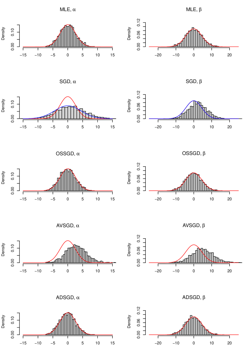
Figure 1: Statistical errors renormalized by $\sqrt{n}$ for MLE, SGD, OSSGD, AVSGD and ADSGD for $n=10^{4}$ and $B=2\times 10^{3}$ Monte-Carlo simulations. Theoretical optimal variance (in red) and variance of SGD (in blue) are superimposed.

	MLE	SGD	OSSGD	AVSGD	ADSGD
time (s)	98.52	30.23	30.40	30.41	43.48

It is worth noting that, for the specific case of the estimation of the parameters in the Gamma distribution, moment estimators (Brouste et al., 2021) or other original explicit estimators (Ye & Chen, 2017) could have been considered as initial guess estimation in the one-step procedure instead of the SGD.

5 Conclusion

In this paper, we propose to apply the one-step procedure to the slowly converging stochastic gradient descent in order to fasten the convergence rate and reach asymptotical efficiency. It is a fast and asymptotically efficient alternative to averaging or adaptivity.

The one-step procedure for the stochastic gradient descent is considered here in the i.i.d. setting but it will be extended in a further work to the regression setting (linear regression, logistic regression (see also (Bercu et al., 2020) for an adaptative procedure), generalized linear models) for larger applications.

Appendix A Robbins-Monro’s algorithm

The proof of Proposition 1 which shows asymptotic normality for the slowly converging stochastic gradient descent method ($\gamma_{i}=i^{-r}$, $1/2<r<1$) in the multidimensional setting follows (Sacks, 1958) and (Ruppert, 1988). The Robbins-Monro algorithm can be rewritten as noisy version of the classical gradient descent method, namely

$$\vartheta_{i+1}=\vartheta_{i}-\gamma_{i}M(\vartheta_{i})-\gamma_{i}\xi_{i},\quad i\geq 1,$$ (11)

where $\xi_{i}=-\nabla_{\vartheta}\log f(X_{i},\vartheta_{i})-M(\vartheta_{i})$. From condition (8), one has

$$\vartheta_{i+1}-\vartheta = \vartheta_{i}-\vartheta-\gamma_{i}\left({\cal I}(\vartheta)(\vartheta_{i}-\vartheta)+\delta_{i}\right)-\gamma_{i}\xi_{i}$$ (12)

$$= (I_{p}-\gamma_{i}{\cal I}(\vartheta))(\vartheta_{i}-\vartheta)-\gamma_{i}\delta_{i}-\gamma_{i}\xi_{i},$$

where $\delta_{i}=\mathrm{o}(\|\vartheta_{i}-\vartheta\|)$. A straightforward induction based on the recursive equation (12) yields

$$\vartheta_{i+1}-\vartheta=\alpha_{0,i}(\vartheta_{1}-\vartheta)-\sum_{j=1}^{i}\gamma_{j}\alpha_{j,i}\delta_{j}-\sum_{j=1}^{i}\gamma_{j}\alpha_{j,i}\xi_{j}$$ (13)

with matrices $\alpha_{j,i}=\prod_{k=j+1}^{i}(I_{p}-\gamma_{k}{\cal I}(\vartheta))$ for $j\neq i$ and $\alpha_{i,i}=I_{p}$.

The covariance matrix $\mathcal{I}(\vartheta)$ is a symmetric positive definite real matrix, it can be diagonalized such that $D(\vartheta)=P^{\mathrm{T}}(\vartheta)\mathcal{I}(\vartheta)P(\vartheta)$ is a diagonal matrix and $P(\vartheta)$ is an orthogonal matrix. Let us denote by $b_{1}$, $b_{2}$, …, $b_{p}$ the eigenvalues of $\mathcal{I}(\vartheta)$ in the deacreasing order.
First, we can remark that

$$K_{1}\exp\left(\frac{b_{p}(j^{1-r}-i^{1-r})}{2(1-r)}\right)\leq\left\|\alpha_{j,i}\right\|_{m}\leq K_{2}\exp\left(\frac{b_{p}(j^{1-r}-i^{1-r})}{2(1-r)}\right),$$

for some positive constants $K_{1}$ and $K_{2}$.

Let us define

$$v_{i}=\left(\sum_{j=1}^{i}\gamma^{2}_{j}\|\alpha_{j,i}\|_{m}^{2}\right)^{-1/2}.$$

It can be shown that $v_{i}\sim i^{r/2}$.
In order to prove the proposition, we have to show successively, when $i\rightarrow\infty$,

$$v_{i}\alpha_{0,i}(\vartheta_{1}-\vartheta)\longrightarrow 0\quad\mbox{in probability\quad{\bf(Step 1)}}$$

$$v_{i}\sum_{j=1}^{i}\gamma_{j}\alpha_{j,i}\xi_{j}\Longrightarrow{\cal N}\left(0,\frac{1}{2}I_{p}\right)\quad\mbox{in law \quad{\bf(Step 2)}}$$

and

$$v_{i}\sum_{j=1}^{i}\gamma_{j}\alpha_{j,i}\delta_{j}\longrightarrow 0\quad\mbox{in probability \quad{\bf(Step 3)}}$$

Slutsky’s theorem concludes the proof of the Proposition. Here are the details for the three steps:

$\diamond$ Step 1:

Using the relation

$$\alpha_{j,i}-\alpha_{j-1,i}=\gamma_{j}{\cal I}(\vartheta)\alpha_{j,i}$$

we show as in (Sacks, 1958) that, for a sequence $W_{i}\rightarrow W$ (which could be $\infty$), we have

$$\sum_{j=m}^{i}\gamma_{j}{\cal I}(\vartheta)\alpha_{j,i}W_{j}\longrightarrow W$$ (14)

as $i$ tends to infinity and finally

$$\lim_{i\rightarrow\infty}v_{i}\alpha_{j,i}=0.$$ (15)

Since the random variable $\vartheta_{1}$ is square integrable, one can easily obtain

$$\mathbb{E}\left[\left\|\alpha_{0,i}(\vartheta_{1}-\vartheta)\right\|\right] \leq K_{3}\left\|\alpha_{0,i}\right\|_{m},$$

where $K_{3}$ is a positive constant. Markov’s inequality and Equation (15) provide the expected convergence.

$\diamond$ Step 2:

The spectral decomposition of $\mathcal{I}(\vartheta)$ introduced above allows to write

$$P^{\mathrm{T}}(\vartheta)\sum_{j=1}^{i}\gamma_{j}\alpha_{j,i}\xi_{j}=\sum_{j=1}^{i}\gamma_{j}\beta_{j,i}\Upsilon_{j},$$

where $\Upsilon_{j}=P^{\mathrm{T}}(\vartheta)\xi_{j}$ and $\beta_{j,i}=\prod_{k=j+1}^{i}(I_{p}-\gamma_{k}D(\vartheta))$. Moreover, the random vectors $\Upsilon_{j}$ are centered, independent and identically distributed with variance matrix

$$\mathbb{E}\left[\Upsilon_{j}\Upsilon_{j}^{\mathrm{T}}\right]=P^{\mathrm{T}}(\vartheta)\mathbb{E}\left[\xi_{j}\xi_{j}^{\mathrm{T}}\right]P(\vartheta)=P^{\mathrm{T}}(\vartheta)\mathcal{I}(\vartheta)P(\vartheta)=D(\vartheta)=\mathrm{diag}\left(b_{1},\ldots,b_{p}\right)$$

which is diagonal.

We can use the same arguments developed in (Ruppert, 1988, Corollary 3.2) to obtain for each coordinate the proper convergence. For instance, one can obtain for the first component

$$\sum_{j=1}^{i}\gamma_{j}(\beta_{j,i}\Upsilon_{j})_{1}=\sum_{j=1}^{i}\gamma_{j}(\beta_{j,i})_{1,1}(\Upsilon_{j})_{1}=-i^{-r}\sum_{j=r(i)}^{i}c(j,i)(\Upsilon_{j})_{1}+o(1)$$

with $r(i)=\lfloor i-K_{4}i^{r}\log i\rfloor$ and $c(j,i)=\exp\left(-b_{1}\sum_{k=j+1}^{i}k^{-r}\right)$. Hence,

$$i^{r/2}\sum_{j=1}^{i}\gamma_{j}(\beta_{j,i}\Upsilon_{j})_{1}\Longrightarrow \mathcal{N}\left(0,1/2\right)$$

in law when $i\rightarrow\infty$. Similar arguments for the other coordinates give the result.

$\diamond$ Step 3:

The upper bound

$$\mathbb{E}\left[\left\|\vartheta_{i}-\vartheta\right\|^{2}\right]\leq K_{5}i^{1-2r}\ \ \ (K_{5}>0)$$

can be found in (Chung, 1954, Theorem 1), which implies that, for $r>\frac{1}{2}$,

$$\mathbb{E}\left[\left\|\delta_{i}\right\|^{2}\right]\longrightarrow 0$$

as $i$ goes to infinity. The expected result of this step follows from convergence in (14).

Appendix B One-step procedure

For an observation sample $(X_{1},\ldots,X_{n})$, let us denote $\ell_{n}(u)=\sum_{i=1}^{n}\log f(X_{i},u)$. Recall that $\vartheta$ is the true parameter and

$$\overline{\vartheta}_{n}=\vartheta_{n}+{\cal I}(\vartheta_{n})^{-1}\cdot\frac{1}{n}\nabla_{u}\ell_{n}(\vartheta_{n}),\quad n\geq 1.$$ (16)

Consistency:

The consistency of the sequence of initial guess estimators gives, as $n\rightarrow\infty$, $\vartheta_{n}\longrightarrow\vartheta$ in probability. Since $\mathbb{E}_{\vartheta}\nabla_{u}\ell_{n}(\vartheta)=0$, the uniform law of large number gives, as $n\rightarrow\infty$,

$$\frac{1}{n}\nabla_{u}\ell_{n}(\vartheta_{n})\longrightarrow 0_{\mathbb{R}^{p}}$$

in probability. The uniform continuity of the Fisher information matrix gives the result. Since the initial stochastic gradient descent is also strongly consistent (Blum, 1954), we can also obtain the strong consistence with the strong law of large number.

Asymptotic normality:

From (16), we have

$$\sqrt{n}\left(\overline{\vartheta}_{n}-\vartheta\right)=\sqrt{n}\left(\vartheta_{n}-\vartheta\right)+{\cal I}(\vartheta_{n})^{-1}\cdot\frac{1}{\sqrt{n}}\nabla_{u}\ell_{n}(\vartheta_{n}).$$

The mean-value theorem gives

$$\nabla_{u}\ell_{n}(\vartheta_{n})=\nabla_{u}\ell_{n}(\vartheta)+\int_{0}^{1}\nabla_{u,u}^{2}\ell_{n}\left(\vartheta+v(\vartheta_{n}-\vartheta)\right)dv\cdot\left(\vartheta_{n}-\vartheta\right)$$

and

$$\sqrt{n}\left(\overline{\vartheta}_{n}-\vartheta\right) =n^{\frac{\delta}{2}}\left\{I_{p}+{\cal I}(\vartheta_{n})^{-1}\frac{1}{n}\int_{0}^{1}\nabla_{u,u}^{2}\ell_{n}\left(\vartheta+v(\vartheta_{n}-\vartheta)\right)dv\right\}n^{\frac{\delta}{2}}\left(\vartheta_{n}-\vartheta\right)n^{\frac{1}{2}-\delta}$$

$$\quad-{\cal I}(\vartheta_{n})^{-1}\cdot\frac{1}{\sqrt{n}}\nabla_{u}\ell_{n}(\vartheta),$$ (17)

where $I_{p}$ is the $p\times p$ identity matrix.
The central limit theorem gives, as $n\rightarrow\infty$,

$$\frac{1}{\sqrt{n}}\nabla_{u}\ell_{n}(\vartheta)\Longrightarrow{\cal N}\left(0,{\cal I}(\vartheta)\right)$$

in law and the proper convergence of the second term in the r.h.s. of Equation (B).

Considering the first right-hand term, we have that $(\vartheta_{n})_{n\geq 1}$ is $n^{\frac{\delta}{2}}$-consistent by assumption and $n^{\frac{1}{2}-\delta}\rightarrow 0$, as $n\rightarrow\infty$, for $\frac{1}{2}<\delta\leq 1$. Then, we need to show that

$$n^{\frac{\delta}{2}}\left(I_{p}+{\cal I}(\vartheta_{n})^{-1}\frac{1}{n}\int_{0}^{1}\nabla_{u,u}^{2}\ell_{n}\left(\vartheta+v(\vartheta_{n}-\vartheta)\right)dv\right)=n^{\frac{\delta}{2}}A$$

is bounded in probability as $n\rightarrow\infty$ with

$$A = {\cal I}(\vartheta_{n})^{-1}\left({\cal I}(\vartheta_{n})+\frac{1}{n}\int_{0}^{1}\nabla_{u,u}^{2}\ell_{n}\left(\vartheta+v(\vartheta_{n}-\vartheta)\right)dv\right)$$

$$= {\cal I}(\vartheta_{n})^{-1}\cdot\left(\left[{\cal I}(\vartheta_{n})-{\cal I}(\vartheta)\right]+\left[\frac{1}{n}\nabla_{u,u}^{2}\ell_{n}(\vartheta)+{\cal I}(\vartheta)\right]\right.$$

$$\left.+\frac{1}{n}\int_{0}^{1}\left[\frac{\partial^{2}}{\partial\vartheta^{2}}\ell_{n}\left(\vartheta+v(\vartheta_{n}-\vartheta)\right)-\nabla_{u,u}^{2}\ell_{n}(\vartheta)\right]dv\right).$$

The second terms in the r.h.s. converges to zero at rate $\sqrt{n}$. The Lipschitz continuity of the Fisher information allows to control the first and third terms by $C\|\vartheta_{n}-\vartheta\|$ where $C$ is a generic constant. Since $(\vartheta_{n})_{n\geq 1}$ is $n^{\frac{\delta}{2}}$-consistent, the quantity $n^{\frac{\delta}{2}}A$ is bounded in probability as $n\rightarrow\infty$. The Slutsky theorem gives the final result.

Acknowledgments

This research partially benefited from the support of the ANR project ’Efficient inference for large and high-frequency data’ (ANR-21-CE40-0021) and the NSF project NSF-DMS 220 47 95.

References

- Abramowitz & Stegun (1992) Abramowitz, M., & Stegun, I. A. (Eds.) (1992). Handbook of mathematical functions with formulas, graphs, and mathematical tables. Dover Publications, Inc., New York.
- Amari (1998) Amari, S. (1998). Natural gradient works efficiently in learning. Neural Computation, 10(2), 251–276.
- Bercu et al. (2020) Bercu, B., Godichon, A., & Portier, B. (2020). An efficient stochastic Newton algorithm for parameter estimation in logistic regressions. SIAM J. Control Optim., 58(1), 348–367.
- Blum (1954) Blum, J. R. (1954). Approximation methods which converge with probability one. Ann. Math. Statist., 25, 382–386.
- Brouste et al. (2021) Brouste, A., Dutang, C., & Mieniedou, D. N. (2021). The R journal: OneStep : Le Cam’s one-step estimation procedure. The R Journal, 13, 383–394.
- Brouste & Farinetto (2023) Brouste, A., & Farinetto, C. (2023). Fast and asymptotically efficient estimation in the Hawkes processes. Jpn. J. Stat. Data Sci., 6(1), 361–379.
- Brouste & Masuda (2018) Brouste, A., & Masuda, H. (2018). Efficient estimation of stable Lévy process with symmetric jumps. Stat. Inference Stoch. Process., 21(2), 289–307.
- Brouste et al. (2020) Brouste, A., Soltane, M., & Votsi, I. (2020). One-step estimation for the fractional Gaussian noise at high-frequency. ESAIM Probab. Stat., 24, 827–841.
- Chung (1954) Chung, K. L. (1954). On a stochastic approximation method. Ann. Math. Statist., 25, 463–483.
- Dabye et al. (2018) Dabye, A. S., Gounoung, A. A., & Kutoyants, Y. A. (2018). Method of moments estimators and multi-step MLE for Poisson processes. Izv. Nats. Akad. Nauk Armenii Mat., 53(4), 31–45.
- Duflo (1997) Duflo, M. (1997). Random iterative models, vol. 34 of Applications of Mathematics (New York). Springer-Verlag, Berlin.
- Dvoretzky (1956) Dvoretzky, A. (1956). On stochastic approximation. In Proc. Third Berkeley Symp. Math. Statist. Prob., vol. 1, (pp. 95–104).
- Fabian (1968) Fabian, V. (1968). On asymptotic normality in stochastic approximation. Ann. Math. Statist., 39, 1327–1332.
- Gloter & Yoshida (2021) Gloter, A., & Yoshida, N. (2021). Adaptive estimation for degenerate diffusion processes. Electron. J. Stat., 15(1), 1424–1472.
- Hodges & Lehmann (1956) Hodges, J. L., Jr., & Lehmann, E. L. (1956). Two approximations to the Robbins-Monro process. In Proc. Third Berkeley Symp. Math. Statist. Prob., vol. 1, (pp. 95–104).
- Kamatani & Uchida (2015) Kamatani, K., & Uchida, M. (2015). Hybrid multi-step estimators for stochastic differential equations based on sampled data. Stat. Inference Stoch. Process., 18(2), 177–204.
- Kutoyants & Motrunich (2016) Kutoyants, Y. A., & Motrunich, A. (2016). On multi-step MLE-process for Markov sequences. Metrika, 79(6), 705–724.
- Lai & Robbins (1979) Lai, T. L., & Robbins, H. (1979). Adaptive design and stochastic approximation. The Annals of Statistics, 7(6), 1196–1221.
- Le Cam (1956) Le Cam, L. (1956). On the asymptotic theory of estimation and testing hypotheses. In Proc. Third Berkeley Symp. Math. Statist. Prob., vol. 1, (pp. 355–368).
- Pelletier (1998) Pelletier, M. (1998). On the almost sure asymptotic behaviour of stochastic algorithms. Stochastic Process. Appl., 78(2), 217–244.
- Pelletier (2000) Pelletier, M. (2000). Asymptotic almost sure efficiency of averaged stochastic algorithms. SIAM J. Control Optim., 39(1), 49–72.
- Polyak & Juditsky (1992) Polyak, B. T., & Juditsky, A. B. (1992). Acceleration of stochastic approximation by averaging. SIAM J. Control Optim., 30(4), 838–855.
- Robbins & Monro (1951) Robbins, H., & Monro, S. (1951). A stochastic approximation method. Ann. Math. Statist., 22, 400–407.
- Ruppert (1988) Ruppert, D. (1988). Efficient estimations from a slowly convergent Robbins-Monro process. Tech. rep., Cornell University.
- Sacks (1958) Sacks, J. (1958). Asymptotic distribution of stochastic approximation procedures. Ann. Math. Statist., 29, 373–405.
- Venter (1967) Venter, J. H. (1967). An extension of the Robbins-Monro procedure. Ann. Math. Statist., 38, 181–190.
- Wolfowitz (1952) Wolfowitz, J. (1952). On the stochastic approximation method of Robbins and Monro. Ann. Math. Statist., 23, 457–461.
- Ye & Chen (2017) Ye, Z.-S., & Chen, N. (2017). Closed-form estimators for the gamma distribution derived from likelihood equations. Amer. Statist., 71(2), 177–181.