In search of a precursor for crystal nucleation of hard and charged colloids

Abstract

The interplay between crystal nucleation and the structure of the metastable fluid has been a topic of significant debate over recent years. In particular, it has been suggested that even in simple model systems such as hard or charged colloids, crystal nucleation might be foreshadowed by significant fluctuations in local structure around the location where the first nucleus arises. We investigate this using computer simulations of spontaneous nucleation events in both hard and charged colloidal particles. To detect local structural variations, we use both standard and unsupervised machine learning methods capable of finding hidden structures in the metastable fluid phase. We track numerous nucleation events for the face-centered cubic and body-centered cubic crystal on a local level, and demonstrate that all signs of crystallinity emerge simultaneously from the very start of the nucleation process. We thus conclude that there is no precursor for the nucleation of charged colloids.

I Introduction

Crystal nucleation plays an important role in fields ranging from colloidal self-assembly, to protein crystallization, and even polymorph selection in pharmaceuticals Karthika, Radhakrishnan, and Kalaichelvi (2016); Sosso et al. (2016). However, despite its importance in a number of essential fields, the detailed mechanism of forming a crystal nucleus still remains a topic of continuous debate.

The simplest theory which addresses crystal nucleation is classical nucleation theory (CNT). In CNT, the metastable fluid is continuously undergoing thermal fluctuations, where small, solid clusters form and dissolve until one appears which is large enough (critically large) to grow out into a macroscopic crystal. The size of such a critical cluster is given simply by balancing the bulk free-energy gain associated with transitioning into the more stable solid phase, with the surface free-energy cost of having a finite crystal cluster immersed in the fluid. This picture, however, becomes significantly more complicated when one considers the possibility of multiple competing crystal structures, typically referred to as polymorphs. In systems with crystal polymorphs, the crystalline phase that first nucleates in the metastable fluid is not necessarily the stable phase. Theories to address such situations, such as the Ostwald step rule Ostwald (1897), and the Alexander-McTague theory Alexander and McTague (1978) have proven unreliable in explaining polymorph selection (see e.g. Refs. Russo and Tanaka, 2012a; Taffs and Patrick Royall, 2016; Ouyang et al., 2016).

One complication when studying such questions is the close interplay between local structural motifs that occur naturally in the fluid, and the ones that might emerge when the crystal forms. It has been suggested that motifs hiding in the fluid are predictive of, or even responsible for, the location or polymorph of the nucleus that forms Russo and Tanaka (2012b); Gispen et al. (2023). To investigate this possibility, one avenue forward could be to explore just how much information the metastable liquid is hiding regarding the nucleation process. Over the last two decades a plethora of studies have appeared presenting contradictory observations ten Wolde and Frenkel (1999); Schilling et al. (2010); Russo and Tanaka (2016); Tan, Xu, and Xu (2014); Li et al. (2020); Russo and Tanaka (2012b); Hu and Tanaka (2022); Lu et al. (2015); Berryman et al. (2016); Tanaka et al. (2019); Lechner, Dellago, and Bolhuis (2011). In particular, in simple systems such as charged colloids which nucleate into either the face-centered cubic (FCC) or body-centered cubic (BCC) crystal, some studies have argued that local structural order develops before the local density increases Russo and Tanaka (2012b); Hu and Tanaka (2022); Lu et al. (2015), while other authors found evidence that the two processes happen simultaneously Berryman et al. (2016).

To address this issue, some recent, intriguing studies have explored how modifying (via biasing) the structure of the fluid – either enhancing or suppressing specific local motifs – affects the nucleation process Hu and Tanaka (2022); Taffs and Patrick Royall (2016). In principle, such studies might be able to give one direct evidence that a specific local structure either enhances or suppresses the nucleation process. Unfortunately, however, biasing the structure of the fluid modifies not only its local structure but also its thermodynamics, meaning that comparisons with the unbiased case are inconclusive.

The more direct route to trying to explore how various kinds of local ordering interplay in crystal nucleation is simply to simulate the nucleation event, and follow the various structural and density features as nucleation happens. At first glance this would appear to be a straightforward approach. However, the challenge in this case lies in the difficulty in creating local order parameters that are unbiased. For example, order parameters that are tuned to recognize the crystalline regions from fluid might struggle at the boundary between the fluid and crystal – a highly important aspect at the beginning of nucleation. Similar issues exist for other order parameters, making it very difficult to pinpoint the start of the nucleation process and hence to determine whether structural order emerges before, during, or after densification. Hence, in some cases instead of capturing accurately whether local structure exists in the highly fluctuating metastable fluid, one ends up examining the properties of the order parameter instead of the properties of the fluid.

While this problem is never fully avoidable, one option to try and avoid accidental biases is to exploit multiple different measures for local order – for instance measures associated with symmetries like bond-order parameters and order associated with the topological connections between neighboring particles – such as topological cluster classification (TCC). Interestingly, new unsupervised machine learning (UML) algorithms also give new avenues to probe structure (see e.g. Refs. Becker et al., 2022; Reinhart et al., 2017; Boattini, Dijkstra, and Filion, 2019; Boattini et al., 2020; Coli and Dijkstra, 2021; van Damme et al., 2020; Gardin et al., 2021; Coslovich, Jack, and Paret, 2022; Paret, Jack, and Coslovich, 2020; Adorf et al., 2019) . Recent studies have even demonstrated that simple, UML-based approaches are able to extract variations in disorder in the structure of supercooled fluids from e.g. a simple vector of bond order parameters Boattini et al. (2020); Paret, Jack, and Coslovich (2020); Coslovich, Jack, and Paret (2022). Intriguingly, this includes identifying variations in local structure that are not easily extracted by looking at each element of the vector individually.

In this paper, we attempt to take the utmost care in identifying local signatures of the fluid and and revisit the question: are there hidden local structures present in metastable fluid that foreshadow the location of the imminent formation of a crystal nucleus? Specifically, we apply both classical and UML-based methods to the nucleation of hard and charged colloids in both the regime of strong screening and weak screening, for which respectively the FCC and BCC crystals nucleate. To this end, we simulate numerous spontaneous nucleation events, and closely follow all nucleation events as a function of time. In particular, similar to Ref. Berryman et al., 2016 we zoom in on the regions where the nuclei are born and analyze the local fluctuations in density and structure of the metastable fluid. By doing this we can locally track whether there is a delay between the increase in local structural ordering and local density prior to the start of nucleation. Such a delay would indicate the presence of a precursor. However, within the limits of this study, we find no evidence of such a precursor in the systems we studied.

II Model

We consider a system of $N$ like-charged hard spheres of diameter $\sigma$ suspended in a solvent containing salt. The effective interaction potential between these colloids is given by the repulsive hard-core Yukawa potential

$$\beta\phi(r)=\begin{dcases}\beta\epsilon\;\frac{e^{-\kappa\sigma(r/\sigma-1)}}{r/\sigma}&\quad\text{for }r\geq\sigma,\\ \infty&\quad\text{for }r<\sigma,\end{dcases}$$ (1)

with contact value $\beta\epsilon=Z^{2}\lambda_{B}/\sigma(1+\kappa\sigma/2)^{2}$, where $Z$ is the charge of the colloids in electron charge, $\lambda_{B}$ is the Bjerrum length, $\kappa$ is the inverse Debye screening length, and $\beta=1/k_{B}T$, with $k_{B}$ the Boltzmann constant and $T$ the temperature. Note that in the limit of zero charge ($Z\to 0$) or infinite screening ($\kappa\sigma\to\infty$), this potential reduces to the hard-sphere potential. The interaction potential was truncated and shifted such that the shift was never more than $10^{-5}k_{B}T$.

Nucleation of both the BCC and FCC phases in this system has been studied in the past (see e.g. Refs. Auer and Frenkel, 2005; Desgranges and Delhommelle, 2007; Browning, Doherty, and Fredrickson, 2008; Gispen and Dijkstra, 2022; de Jager and Filion, 2022). In a previous study de Jager and Filion (2022), we used umbrella sampling to calculate the nucleation barriers and rates of highly screened charged particles. In this paper, we will study the nucleation of some of these (nearly-)hard systems, as well as the nucleation of weakly screened charged particles. To be able to compare the nucleation processes of different systems, we select state points with approximately equal barrier heights. In particular, we will simulate brute-force nucleation events of systems with barrier heights around 15-18$k_{B}T$. Information on the nucleation barriers of the systems studied is given in Tab. 1. Note that systems with a Debye screening length of $1/\kappa\sigma=0.01$ were found to behave essentially as “hard” spheres when mapped with an effective hard-sphere diameter de Jager and Filion (2022). A brief explanation of the methods used for computing the nucleation barriers as well as some additional information on these systems can be found in the Supplemental Materials (SM).

Table 1: For each system studied, the packing fraction of the supersaturated fluid $\eta^{*}$ at which the brute force nucleation is performed together with the corresponding supersaturation $\beta|\Delta\mu|$. The last columns give the critical nucleus size $n^{*}$ and barrier height $\beta\Delta G^{*}$ obtained using umbrella sampling. The error in $\beta\Delta G^{*}$ is no more than 1.

	$\beta\epsilon$	$1/\kappa\sigma$	$\eta^{*}$	$\beta|\Delta\mu|$	$n^{*}$	$\beta\Delta G^{*}$
FCC	hard spheres		0.5385	0.585	75	16.5
	81	0.01	0.4681	0.584	84	16.3
	8	0.04	0.4400	0.541	69	14.8
BCC	81	0.40	0.1305	0.321	122	18.0

III Methods

To explain the methods we use for studying the nucleation events, we need to discuss two things: i) how we identify local structure, and ii) how we track nucleation events locally.

III.1 Identifying local structure

We use three different methods to classify the local structure. The first method considers just the averaged bond-orientational order parameters (BOPs) of Lechner and Dellago Lechner and Dellago (2008). For this, we first calculate for each particle $i$ the complex quantities

$$q_{lm}(i)=\frac{1}{N_{b}(i)}\sum_{j\in\mathcal{N}_{b}(i)}Y_{l}^{m}(\theta_{ij},\phi_{ij}),$$ (2)

where $\mathcal{N}_{b}(i)$ is the set of the $N_{b}(i)$ nearest neighbors of particle $i$, $\,Y_{lm}\left(\theta,\phi\right)$ are the spherical harmonics with $m\in[-l,l]$, and $\theta_{ij}$ and $\phi_{ij}$ are the polar and azimuthal angles of the vector $\mathbf{r}_{ij}=\mathbf{r}(j)-\mathbf{r}(i)$ connecting particles $i$ and $j$. We use the SANN algorithm van Meel et al. (2012) to determine the nearest neighbors. Next, we average these complex quantities over the set of nearest neighbors as well as the particle itself

$$\bar{q}_{lm}(i)=\frac{1}{N_{b}(i)+1}\sum_{j\in\{i,\mathcal{N}_{b}(i)\}}q_{lm}(j).$$ (3)

Finally, we compute the rotationally invariant averaged BOPs

$$\bar{q}_{l}(i)=\sqrt{\frac{4\pi}{2l+1}\sum_{m=-l}^{l}|\bar{q}_{lm}(i)|^{2}},$$ (4)

and

$$\bar{w}_{l}(i)=\frac{w_{l}(i)}{\left(\sum_{m=-l}^{l}|\bar{q}_{lm}(i)|^{2}\right)^{3/2}},$$ (5)

with

$$w_{l}(i)=\!\!\!\!\!\!\sum_{\begin{matrix}\scriptstyle m_{1},m_{2},m_{3}\\ \scriptstyle m_{1}+m_{2}+m_{3}=0\end{matrix}}\!\!\!\!\!\!\begin{pmatrix}l&l&l\\ m_{1}&m_{2}&m_{3}\end{pmatrix}q_{lm_{1}}(i)q_{lm_{2}}(i)q_{lm_{3}}(i),$$ (6)

where the term in brackets is the Wigner $3j$ symbol, which is only non-zero when $m_{1}+m_{2}+m_{3}=0$. Note that $w_{l}=0$ when $l$ is odd. Depending on the choice of $l$, these BOPs are sensitive to different (crystal) symmetries. For example, $\bar{q}_{6}$ is very helpful in distinguishing more fluid-like environments from more solid-like environments such as FCC and BCCLechner and Dellago (2008).

While the BOPs are extremely useful for detecting specific symmetries in the local structure of the fluid, they are not necessarily optimal for detecting the most important structural variations in disordered systems such as the metastable fluid. Recent work has shown that BOPs in combination with unsupervised machine learning algorithms is highly effective at autonomously detecting variations that might be difficult to see by studying the individual BOPs Boattini, Dijkstra, and Filion (2019); Boattini et al. (2020). Hence, for the second method, we use an unsupervised algorithm to autonomously detect local structural fluctuations in the metastable fluid. In Ref. Boattini, Dijkstra, and Filion, 2019, Boattini et al. showed that a neural-network-based autoencoder, which is given $\bar{q}_{l}$ with $l\in[1,8]$ as input, does a good job in distinguishing a whole range of different local structures. Similarly, in Ref. van Damme et al., 2020 van Damme et al. showed that using principal component analysis (PCA) as dimensionality reduction method also does a good job in distinguishing the sizable assortment of crystal structures formed by rounded tetrahedra. For our system we found that PCA and an autoencoder preformed equally well in distinguishing order, and hence chose to use the simpler PCA algorithm in our analysis. To specifically focus on finding local fluctuations or signatures in the metastable fluid, we train the PCA model on $\bar{q}_{l}$ with $l\in[1,8]$ of configurations containing only fluid particles and no (significant) solid nuclei. We then use this trained PCA model to analyze the entire nucleation trajectory. Note that in this way, the first principal component corresponds to the largest BOPs-related structural variation in the metastable fluid.

For the third and last method, we use an altogether different approach for classifying local structure. In particular we use the topological cluster classification (TCC) algorithm developed by Malins et al. Malins et al. (2013) to detect any local motifs that the BOPs might have overlooked. More specifically, we use TCC to calculate the population of certain types of clusters, as well as the number of clusters of a certain type a particle is involved in.

Note that for computing the nucleation barriers, we additionally need a binary classification method which labels a particle as either fluid or solid. For this we use the 6-fold Ten Wolde bonds ten Wolde, Ruiz-Montero, and Frenkel (1996)

$$d_{6}(i,j)=\frac{\sum_{m=-6}^{m=6}q_{6m}(i)q_{6m}^{*}(j)}{\sqrt{\left(\sum_{m=-6}^{m=6}|q_{6m}(i)|^{2}\right)\left(\sum_{m=-6}^{m=6}|q_{6m}(j)|^{2}\right)}},$$ (7)

where ^∗ indicates the complex conjugate and $q_{6m}$ are the bond-orientational order parameters given by Eq. (2). Particle $i$ is classified as solid if it has 6 or more neighboring particles $j$ with which it has a solid-like bond, i.e. $d_{6}(i,j)>0.7$. We also use this fluid-solid classification to initially locate and follow the nucleation event. However, we want to point out that, although this provides a general overview of the nucleation event, it is not an ideal order parameter to study the onset of nucleation. Its binary nature with the thresholds for $d_{6}(i,j)$ and the number of solid-like bonds causes it to overlook subtle increases in the local structural ordering of the fluid and hence reacts more slowly to the nucleation than other continuous order parameters.

III.2 Simulating and tracking nucleation events

To obtain the spontaneous nucleation events we use brute force MC, KMC, and MD simulations in the $NVT$-ensemble, where we simulate $N=10976$ and $N=11664$ particles for the systems forming the FCC and BCC phase, respectively. The difference between the MC and KMC simulations is the acceptance ratio of the trial particle moves. For the MC simulations this acceptance ratio is around 30%, whilst for the KMC simulations it is around 85% resulting in dynamics that mimic Brownian motion Sanz and Marenduzzo (2010). The MD simulations are performed using LAMMPS with a Nose-Hoover thermostat Plimpton (1995). We only perform MD simulations for the soft hard-core Yukawa system, i.e. the one with $1/\kappa\sigma=0.40$. As this system does not feel its hard core, it can simply be ignored. Once we have obtained the numerous nucleation events, we want to track the local density and structure to determine if there is a difference between the increase in local structural ordering and local density at the start of nucleation. To this end, for each nucleation event we find the position $\mathbf{r}_{0}$ that best captures the center of the nucleus at the start of nucleation. For this we use the average center-of-mass of the precritical nucleus as a starting point and, if needed, by eye adjust it to best capture the birthplace of the crystal nucleus. Next, for each snapshot of the nucleation trajectory, starting well before the start of nucleation, we determine all particles inside a sphere of radius $R$ around $\mathbf{r}_{0}$, and take the average of the local properties of these particles. This is similar to what Berryman et al. did in Ref. Berryman et al., 2016. The local structural properties that we consider are explained in the previous subsection. Additionally, we define for each particle a local packing fraction measured via the volume of its Voronoi cell. The volumes of the Voronoi cells were obtained using voro++ Rycroft (2009). As we are searching for local precursors, we choose $R$ such that the selected region contains around 30-40 particles. This size provides a good balance between being large enough to obtain relatively stable averages of the local properties, and being small enough to ensure that the averaged properties still represent the local situation.

IV Results

IV.1 Structure of the metastable fluid

Before we look into the actual crystal nucleation, we first characterize the structural properties of the metastable fluid.

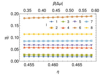
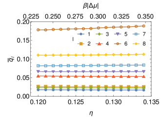
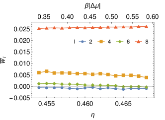
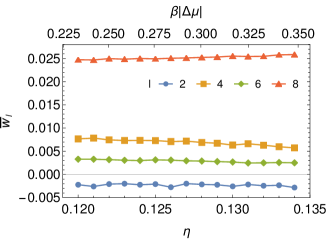
First, we examine the globally averaged values of the local BOPs, and plot the results in Fig. 1 for the metastable fluids of essentially hard spheres and of soft spheres as a function of the supersaturation. We see that $\bar{q}_{6}$, $\bar{q}_{8}$, and $\bar{w}_{8}$ are most prominent in both metastable fluids, and that all BOPs are only marginally affected by the increase in supersaturation. Furthermore, notice that the values in both systems are surprisingly similar, even though the metastable fluid of essentially hard spheres later forms an FCC crystal, whereas the fluid of the soft spheres will form a BCC crystal. The most prevalent difference between the two systems can be found in $\bar{w}_{6}$, which is smaller for the nearly-hard spheres than for soft spheres, and for high supersaturation even becomes on average negative for the nearly-hard spheres whereas it stays positive for the soft spheres. See the SM for more analysis on the $\bar{w}_{l}$’s. We, thus, conclude that the fluid’s “knowledge” about which crystal phase it should nucleate into is difficult to distinguish from the global values of the BOPs.

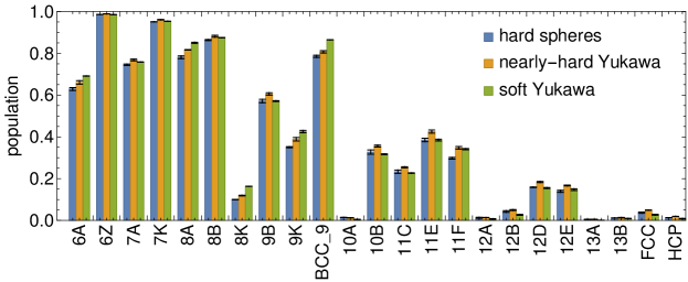
In addition to the BOPs, we take a look at the presence of the different TCC clusters in the metastable fluids. Figure 2 shows the population of various TCC clusters in the metastable fluid of hard spheres, and soft spheres. Even though we see some small deviations in the populations of the different metastable fluids – e.g. clusters 6A, 8A, 8K, 9K, and BCC_9 have a slightly higher population in the fluid of soft spheres and 9B, 10B, 11C, 11E, and 12D have a slightly higher population in the fluid of nearly-hard spheres – the values are again surprisingly similar. This indicates once more that it is difficult to determine which crystal phase will nucleate from the metastable fluid for the systems studied here.

a)		b)
c)		d)

Figure 1: The mean of a,b) the first eight $\bar{q}_{l}$’s and c,d) the first four even $\bar{w}_{l}$’s as a function of the supersaturation for the metastable fluids of hard-core Yukawa with a,c) $\beta\epsilon=81$ and $1/\kappa\sigma=0.01$, and b,d) $\beta\epsilon=81$ and $1/\kappa\sigma=0.40$.

Figure 2: The population of various TCC clusters in the metastable fluids of hard spheres ($\eta=0.5385$), nearly-hard hard-core Yukawa particles ($\beta\epsilon=8$, $1/\kappa\sigma=0.04$, $\eta=0.4400$), and soft hard-core Yukawa particles ($\beta\epsilon=81$, $1/\kappa\sigma=0.40$, $\eta=0.1305$).

Figure 3: PCA on the metastable fluids of a,b) hard spheres ($\eta=0.5385$) and c,d) soft hard-core Yukawa particles ($\beta\epsilon=81$, $1/\kappa\sigma=0.40$, $\eta=0.1305$). a,c) give the weight of each BOP in the first and second principal component. b,d) show the distribution of the fluid particles in the PC1-PC2 plane, with the addition of the corresponding bulk FCC phase of hard spheres ($\eta=0.5981$) and bulk BCC phase of soft hard-core Yukawa ($\beta\epsilon=81$, $1/\kappa\sigma=0.40$, $\eta=0.1311$). e) Pearson correlation between PC1 and the number of TCC clusters a particle is involved in for the hard spheres. The color of the bars indicate clusters that consist of one or more tetrahedral subclusters (blue), one or more square pyramidal subclusters (yellow), or both/neither (gray).

a)             $\eta$	b)            PC1	c)            9B	d)            11F

Figure 4: Snapshot of the metastable fluid of hard spheres ($\eta=0.5385$) colored by a) the local packing fraction, b) the first principal component, c) the number of 9B clusters per particle, and d) the number of 11F clusters per particle.

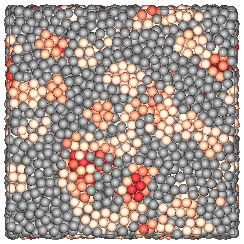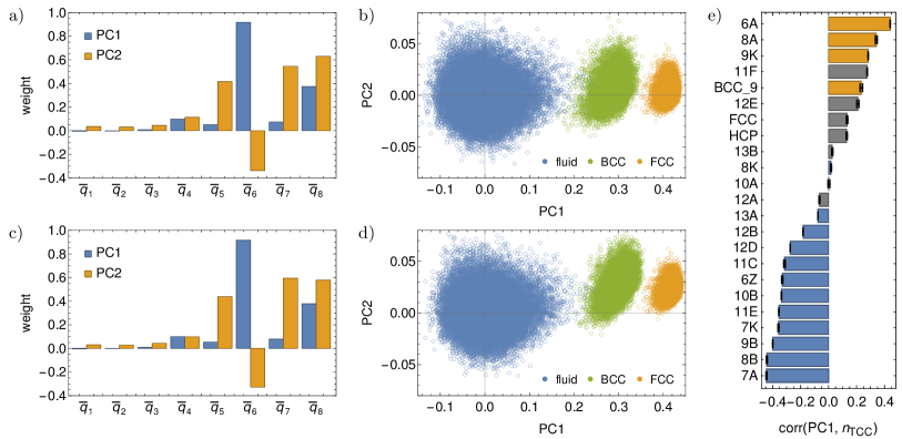
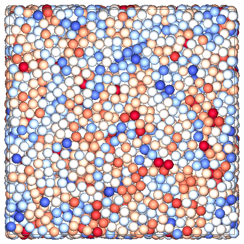
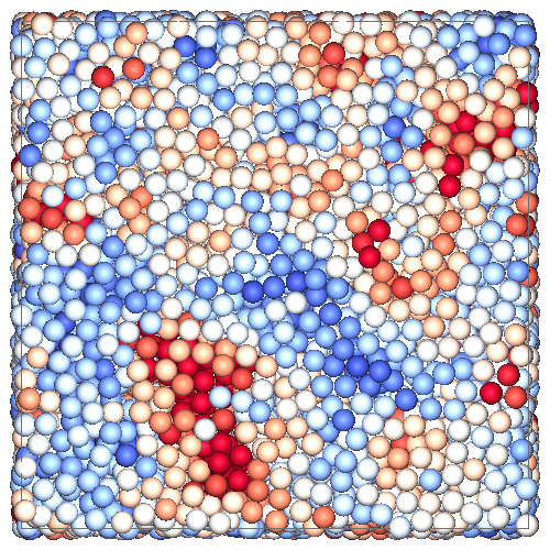
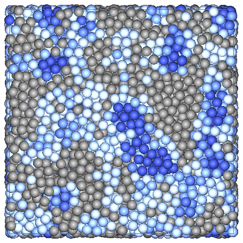
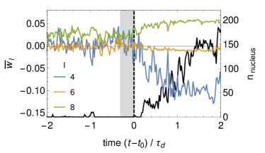
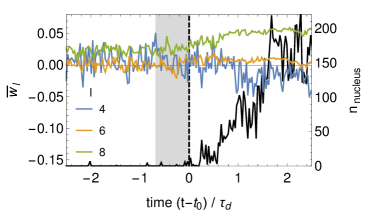
Next, we characterize the local ordering of the metastable fluid on the single-particle level. As explained in the Methods, we train a PCA model using only configurations of the metastable fluid. In all cases the first principal component (PC1) explains around 70% of the total variance of the input. To illustrate what kind of fluctuations PCA picks up in the fluid, Figs. 3a,c) show for the metastable fluids of hard spheres and of soft spheres the weight of each BOP in the first and second principal component. We see that PC1 is mostly made up of $\bar{q}_{6}$ and $\bar{q}_{8}$. Furthermore, Figs. 3b,d) show the distribution of these metastable fluid particles in the PC1-PC2 plane, as well as the distributions of the corresponding FCC and BCC phase. (Recall that the data for the crystalline particles was not used in training the PCA models.) In this scatter plot we can neatly see that the crystal phases lie in the region of large PC1. To get a better understanding of the real-space distribution of these particles with above or below average PC1, we take a look at a single snapshot of the metastable fluid of hard spheres and color the particles according to their local packing fraction, PC1, and the number of 9B and 11F clusters a particles is involved in, see Fig. 4. Even though the spatial correlations in the local packing fraction are not clearly visible, we can clearly distinguish by eye large spatial regions of above or below average PC1. The autocorrelation functions of these spatial correlations can be found in the SM. Notice that the regions with above average PC1 correspond to an absence of 9B clusters and a high presence of 11F clusters, while regions with below average PC1 correspond to a high presence of 9B clusters and an absence of 11F clusters. Thus, there is a negative correlation between PC1 and 9B clusters and positive correlation between PC1 and 11F. The precise correlations of these two and other TCC clusters with PC1 are shown in Fig. 3e). Analogous to what was found in Ref. Boattini et al., 2020, the TCC clusters can be roughly divided into two groups: those with a negative correlation, which essentially are all clusters consisting of one or more tetrahedral subclusters, and those with a positive correlation, which contain the clusters consisting of one or more square pyramidal subclusters.

a)		b)

Figure 5: Autocorrelation function of the first and second principal components and the local packing fraction in the metastable fluids of a) hard spheres ($\eta=0.5385$) and b) soft hard-core Yukawa particles ($\beta\epsilon=81$, $1/\kappa\sigma=0.40$, $\eta=0.1305$). The different dashing and darkness of the color indicate the simulation method, and the time is in terms of the long-time diffusion time $\tau_{d}$.

a) $\;\quad(t-t_{0})/\tau_{d}=-0.18$	b) $\;\quad(t-t_{0})/\tau_{d}=0.40$	c) $\;\quad(t-t_{0})/\tau_{d}=0.96$	d) $\;\quad(t-t_{0})/\tau_{d}=1.43$

Figure 6: Four snapshots of a typical nucleation event of hard spheres ($\eta=0.5385$). Here $t_{0}$ indicates the start of nucleation. Fluid particles are displayed at a quarter of their actual size to make the nucleus visible, and red indicates the particles inside the studied region, i.e. those inside the sphere of radius $R$ around the center of nucleation $\mathbf{r}_{0}$.

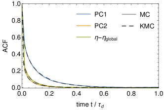
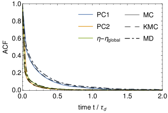
Combining the observation of large spatial regions of above average PC1 with the proximity of these particles to the crystal phases in the PC1-PC2 scatter plot (Fig. 3), we can conclude that regions of above average PC1 form a good candidate for harboring a precursor for crystal nucleation. In the next section, we will investigate these regions whilst tracking the nucleation events. However, before we turn our attention to that, we need to determine the temporal correlations of the local structure such that we know the time window before the start of nucleation during which we can search for a precursor. Figure 5 shows, for multiple simulation methods, the autocorrelation functions (ACFs) of the first two principal components and the local packing fraction in the metastable fluids of hard spheres and of soft spheres. Here, we give the time in terms of the long-time diffusion time $\tau_{d}=\sigma^{2}/6D_{l}$, where $D_{l}$ is the long-time diffusion coefficient obtained from the mean-squared displacement. Notice that the ACFs are essentially independent of the simulation method, which confirms that the dynamics are also independent of the choice of simulation method. We see in both systems that PC2 and the local packing fraction decay extremely fast in time. Although PC1 decays more slowly, i.e. within half a diffusion time for the hard spheres and one diffusion time for the soft spheres, this is still relatively fast. The decay time of PC1 provides a good estimate for the time window before the start of nucleation in which we can search for a precursor.

a)		b)
c)		d)
e)		f)
g)		h)

Figure 7: Left: typical nucleation event of hard spheres ($\eta=0.5385$), same as in Fig. 6. Right: typical nucleation event of soft hard-core Yukawa particles ($\beta\epsilon=81$, $1/\kappa\sigma=0.40$, $\eta=0.1305$). Both events were obtained using MC simulations. The vertical dashed line in each figure indicates the start of nucleation $t_{0}$, and the shaded area indicates the time window before $t_{0}$ for which the ACF of PC1 $>0.05$ (see Fig. 5). In a-f) the black line (right axis) gives the size of the biggest nucleus present in the studied region. The other lines give the average value of a-b) $\bar{q}_{l}$ for $l\in[3,8]$, c-d) $\bar{w}_{l}$ for $l\in[4,6,8]$, e-f) PC1. In g-h) the blue line (right axis) gives PC1, while the yellow line (left axis) gives the local packing fraction $\eta_{\text{local}}$. Note that in e-g) the horizontal dashed lines give the reference value of PC1 in the fluid and solid phase. In g) the right axis is scaled in such a way that the reference values in the fluid and solid of PC1 and $\eta_{\text{local}}$ lie on top of each other. In h) the horizontal dashed lines give the reference value of $\eta_{\text{local}}$ in the fluid and solid phase.

a)		b)
c)		d)
e)		f)
g)		h)

Figure 8: For the same events as in Fig. 7, i.e. hard spheres (left) and soft hard-core Yukawa particles (right), the average number of clusters per particle (left axis, yellow) for a couple of TCC clusters together with the average value of PC1 (right axis, blue). The horizontal dashed lines indicate the reference values of the number of clusters per particle and PC1 in the fluid. In a-f) the left axis is scaled in such a way that these lines lie on top of each other. In g-h) this was not possible without inverting one of the axes.

IV.2 Nucleation study

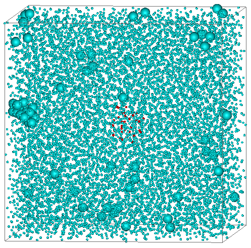
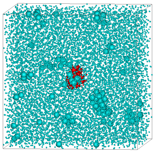
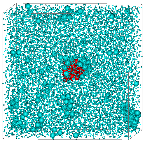
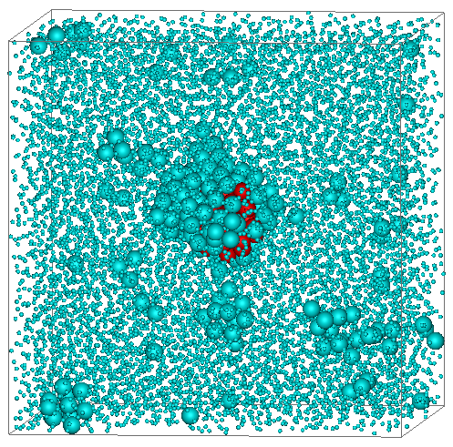
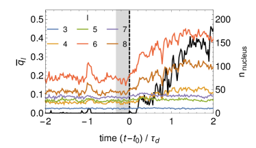
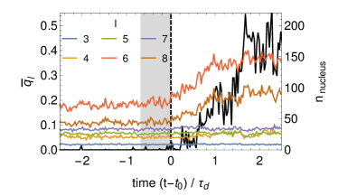
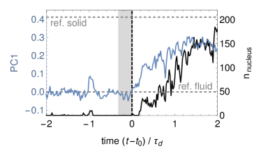
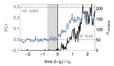
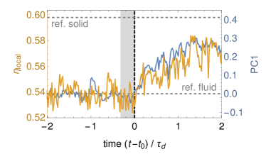
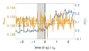
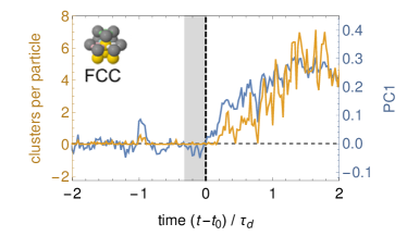
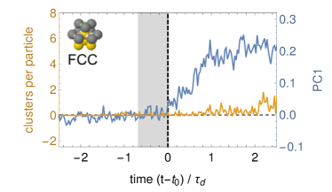
We now turn our attention to crystal nucleation. As explained in the methods, we simulate numerous spontaneous nucleation events using (K)MC and MD simulations, and track for all these events the local properties of the region where nucleation starts. Here, we discuss our observations using two typical nucleation events: one of the hard-spheres system and one of soft spheres ($\beta\epsilon=81$, $1/\kappa\sigma=0.40$). Both these nucleation events were obtained using MC simulations. More nucleation events, where we either used other simulation methods or studied the other systems mentioned in Tab. 1, can be found in the SM. To better illustrate which region we study while tracking a nucleation event, Fig. 6 shows a couple of snapshots of the nucleation event of hard spheres where the particles inside the studied region are colored red. Figure 7 shows for this event and the nucleation event of soft spheres the average properties of the particles in this studied region. Before we discuss what we see, let us again point out that the nucleus size (black line) is not an ideal order parameter for tracking nucleation since its binary nature causes it to overlook subtle increases in the local structural ordering at the onset of nucleation. It does, however, provide a general overview of the nucleation event, such as when the nucleus reaches its critical size (see Tab. 1). That being said, let us first discuss the BOPs of the studied region. We observe no notable change in the behavior of the BOPs before the start of nucleation, but, as soon as nucleation starts, we see a sharp increase in the values of $\bar{q}_{6}$ and $\bar{q}_{8}$ for both systems. Furthermore, for the hard spheres, we see that, once nucleation starts, $\bar{q}_{4}$ increases, $\bar{w}_{6}$ stays negative, and $\bar{w}_{4}$ decreases. This all indicates that indeed the FCC phase nucleates. On the other hand, for the soft spheres, we see that as nucleation starts $\bar{q}_{4}$ barely increases, $\bar{w}_{6}$ stays positive, and $\bar{w}_{4}$ keeps fluctuating around zero, which all indicates that indeed the BCC phase nucleates. Similar to the behavior of the BOPs, we observe no notable change in the behavior of PC1 before the start of nucleation, but see a sharp increase in its value once nucleation starts. Note that this increase in PC1 is visible before the number of particles classified as crystalline starts to rise (black line), demonstrating that PC1 is a better order parameter for tracking the start of nucleation than the nucleus size according to our definition. Lastly, for the hard spheres, we see that the local packing fraction increases simultaneously with PC1 as soon as nucleation starts, and that no notable behavior can be observed before the start of nucleation. This strongly indicates that increase in structural ordering and local density go together and, thus, that there is no apparent precursor. Unfortunately, as the difference between the packing fraction of the fluid and solid phases is extremely small for the soft spheres, i.e. less than 0.001, it is not possible to observe any increase in the local packing fraction on top of the normal fluctuations. Hence, we cannot draw any conclusions on the local packing fraction of the soft spheres.

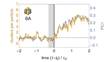
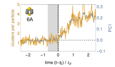
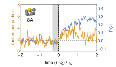
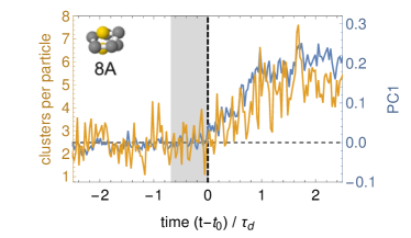
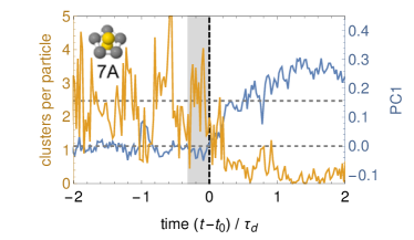
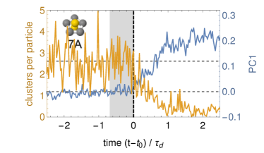
Next, to show that we have missed no subtle changes in the local structure and thus confirm that there is no precursor for nucleation, we further examine the local structure using TCC. In Fig. 8 we show for four of the most relevant TCC clusters the average number of clusters a particle is involved in and compare it with PC1. These four clusters are: i) 6A, which has the strongest positive correlation with PC1 and is present in both bulk FCC and bulk BCC, ii) 8A, which has the second strongest positive correlation with PC1 and is present in bulk BCC but not bulk FCC, iii) FCC, which is present in bulk FCC but not bulk BCC, and iv) 7A, which has the strongest negative correlation with PC1 and can neither be found in bulk FCC nor bulk BCC. Similar figures of other TCC clusters can be found in the SM. For all clusters we see that there is no significant change prior to the start of nucleation. Furthermore, we see that the trends of the 6A cluster coincide almost perfectly with those of PC1. Similarly, we see that the trends of the 8A cluster closely follow the trends of PC1. However, for hard spheres the initial increase in 8A clusters is followed by a decrease. Since 8A is a cluster that is usually found in bulk BCC and not in bulk FCC, this initial increase might be surprising. This can be explained via the observation that 8A clusters are found in high concentrations near the surface of growing nucleiGispen et al. (2023). As a result, the number of these clusters decreases once the nucleus grows beyond our averaging radius. For the FCC cluster, we observe a sharp increase during the nucleation of hard spheres. Notice, however, that this increase starts slightly later than the increase in PC1. This is not surprising as the FCC cluster is a relatively large cluster, i.e. it contains 13 particles, and consequently is not present in the first stages of nucleation. For the soft spheres there is no significant increase in FCC clusters, as expected. Lastly, we take a look at the 7A cluster. In contrast to the other three clusters, this five-fold symmetric cluster has a strong negative correlation with PC1. Moreover, it is strongly present in the metastable fluid phases, whereas its presence in the FCC and BCC phases is negligible. It is, therefore, not surprising that we observe an immediate and sharp decrease in 7A clusters as soon as nucleation starts.

V Conclusions

To conclude, we have characterized the local structure of various metastable fluids of charged colloids using multiple methods: bond-orientational order parameters (BOPs), principal component analysis (PCA) on the BOPs, and topological cluster classification (TCC). In doing this have attempted to avoid artefacts due to biases in our chosen order parameters. For all systems we have found that any local structural ordering has a relatively short lifetime, resulting in a short time window prior to the start of nucleation in which a precursor could exist. By tracking the local structure of the spatial region coinciding with the birthplace of the crystal nucleus, we show that inside this time window no atypical behavior in the local structural order is observed using any of our structural order parameters. Furthermore, we demonstrate that all structural characteristics that differ significantly between the fluid and crystal phase start changing simultaneously as soon as nucleation starts. Specifically in the case of FCC, this includes the local density, which starts growing immediately as soon as structural order emerges. We, thus, conclude that we find no evidence for a precursor for the crystal nucleation of hard and charged colloids.

VI Acknowledgements

L.F. and M.d.J. acknowledge funding from the Vidi research program with project number VI.VIDI.192.102 which is financed by the Dutch Research Council (NWO).

References

- Karthika, Radhakrishnan, and Kalaichelvi (2016) S. Karthika, T. Radhakrishnan, and P. Kalaichelvi, Crystal Growth & Design 16, 6663 (2016).
- Sosso et al. (2016) G. C. Sosso, J. Chen, S. J. Cox, M. Fitzner, P. Pedevilla, A. Zen, and A. Michaelides, Chemical reviews 116, 7078 (2016).
- Ostwald (1897) W. Ostwald, Zeitschrift für physikalische Chemie 22, 289 (1897).
- Alexander and McTague (1978) S. Alexander and J. McTague, Phys. Rev. Lett. 41, 702 (1978).
- Russo and Tanaka (2012a) J. Russo and H. Tanaka, Soft Matter 8, 4206 (2012a).
- Taffs and Patrick Royall (2016) J. Taffs and C. Patrick Royall, Nat. Commun. 7, 13225 (2016).
- Ouyang et al. (2016) W. Ouyang, C. Fu, Z. Sun, and S. Xu, Phys. Rev. E 94, 042805 (2016).
- Russo and Tanaka (2012b) J. Russo and H. Tanaka, Sci. Rep. 2, 1 (2012b).
- Gispen et al. (2023) W. Gispen, G. M. Coli, R. van Damme, C. P. Royall, and M. Dijkstra, ACS Nano 17, 8807–8814 (2023).
- ten Wolde and Frenkel (1999) P. R. ten Wolde and D. Frenkel, Physical Chemistry Chemical Physics 1, 2191 (1999).
- Schilling et al. (2010) T. Schilling, H. J. Schöpe, M. Oettel, G. Opletal, and I. Snook, Phys. Rev. Lett. 105, 025701 (2010).
- Russo and Tanaka (2016) J. Russo and H. Tanaka, J. Chem. Phys. 145, 211801 (2016).
- Tan, Xu, and Xu (2014) P. Tan, N. Xu, and L. Xu, Nat. Phys. 10, 73 (2014).
- Li et al. (2020) M. Li, Y. Chen, H. Tanaka, and P. Tan, Science advances 6, eaaw8938 (2020).
- Hu and Tanaka (2022) Y.-C. Hu and H. Tanaka, Nat. Commun. 13, 4519 (2022).
- Lu et al. (2015) Y. Lu, X. Lu, Z. Qin, and J. Shen, Solid State Communications 217, 13 (2015).
- Berryman et al. (2016) J. T. Berryman, M. Anwar, S. Dorosz, and T. Schilling, J. Chem. Phys. 145, 211901 (2016).
- Tanaka et al. (2019) H. Tanaka, H. Tong, R. Shi, and J. Russo, Nature Reviews Physics 1, 333 (2019).
- Lechner, Dellago, and Bolhuis (2011) W. Lechner, C. Dellago, and P. G. Bolhuis, Phys. Rev. Lett. 106, 085701 (2011).
- Becker et al. (2022) S. Becker, E. Devijver, R. Molinier, and N. Jakse, Phys. Rev. E 105, 045304 (2022).
- Reinhart et al. (2017) W. F. Reinhart, A. W. Long, M. P. Howard, A. L. Ferguson, and A. Z. Panagiotopoulos, Soft Matter 13, 4733 (2017).
- Boattini, Dijkstra, and Filion (2019) E. Boattini, M. Dijkstra, and L. Filion, J. Chem. Phys. 151, 154901 (2019).
- Boattini et al. (2020) E. Boattini, S. Marín-Aguilar, S. Mitra, G. Foffi, F. Smallenburg, and L. Filion, Nat. Commun. 11, 1 (2020).
- Coli and Dijkstra (2021) G. M. Coli and M. Dijkstra, ACS nano 15, 4335 (2021).
- van Damme et al. (2020) R. van Damme, G. M. Coli, R. van Roij, and M. Dijkstra, ACS nano 14, 15144 (2020).
- Gardin et al. (2021) A. Gardin, C. Perego, G. Doni, and G. M. Pavan, arXiv (2021).
- Coslovich, Jack, and Paret (2022) D. Coslovich, R. L. Jack, and J. Paret, J. Chem. Phys. 157, 204503 (2022).
- Paret, Jack, and Coslovich (2020) J. Paret, R. L. Jack, and D. Coslovich, J. Chem. Phys. 152, 144502 (2020).
- Adorf et al. (2019) C. S. Adorf, T. C. Moore, Y. J. Melle, and S. C. Glotzer, J. Phys. Chem. B 124, 69 (2019).
- Auer and Frenkel (2005) S. Auer and D. Frenkel, Adv. Comput. Simul. 173, 149 (2005).
- Desgranges and Delhommelle (2007) C. Desgranges and J. Delhommelle, The Journal of chemical physics 126, 054501 (2007).
- Browning, Doherty, and Fredrickson (2008) A. R. Browning, M. F. Doherty, and G. H. Fredrickson, Physical Review E 77, 041604 (2008).
- Gispen and Dijkstra (2022) W. Gispen and M. Dijkstra, Physical Review Letters 129, 098002 (2022).
- de Jager and Filion (2022) M. de Jager and L. Filion, J. Chem. Phys. 157, 154905 (2022).
- Lechner and Dellago (2008) W. Lechner and C. Dellago, J. Chem. Phys. 129, 114707 (2008).
- van Meel et al. (2012) J. A. van Meel, L. Filion, C. Valeriani, and D. Frenkel, J. Chem. Phys. 136, 234107 (2012).
- Malins et al. (2013) A. Malins, S. R. Williams, J. Eggers, and C. P. Royall, J. Chem. Phys. 139, 234506 (2013).
- ten Wolde, Ruiz-Montero, and Frenkel (1996) P. R. ten Wolde, M. J. Ruiz-Montero, and D. Frenkel, Faraday Discuss. 104, 93 (1996).
- Sanz and Marenduzzo (2010) E. Sanz and D. Marenduzzo, J. Chem. Phys. 132, 194102 (2010).
- Plimpton (1995) S. Plimpton, J. Comp. Phys. 117, 1 (1995).
- Rycroft (2009) C. Rycroft, Chaos 19, 041111 (2009).