Nonlinear multi-state tunneling dynamics in a spinor Bose-Einstein condensate

Abstract

We present an experimental realization of dynamic self-trapping and non-exponential tunneling in a multi-state system consisting of ultracold sodium spinor gases confined in moving optical lattices. Taking advantage of the fact that the tunneling process in the sodium spinor system is resolvable over a broader dynamic energy scale than previously observed in rubidium scalar gases, we demonstrate that the tunneling dynamics in the multi-state system strongly depends on an interaction induced nonlinearity and is influenced by the spin degree of freedom under certain conditions. We develop a rigorous multi-state tunneling model to describe the observed dynamics. Combined with our recent observation of spatially-manipulated spin dynamics, these results open up prospects for alternative multi-state ramps and state transfer protocols.

I Introduction

The phenomenon of tunneling has been widely studied in a range of physical systems including Josephson junctions ryu2013experimental ; mullen1988combined , superfluid annular rings eckel2014hysteresis ; ramanathan2011superflow ; fetter1967low , waveguides khomeriki2010nonlinear , and Bose-Einstein condensates (BECs) zhang2019nonlinear ; guan2020nonexponential ; Arimondo_2007 ; trimborn2010nonlinear ; koller2016nonlinear ; albiez2005direct ; abbarchi2013macroscopic ; chen2011many . In each of these examples, the tunneling description was reduced, after appropriate approximations, to a nonlinear two-state model wherein a control parameter is ramped linearly at a rate $\alpha$ across a transition region where the two asymptotically uncoupled states are coupled. In the absence of interactions, i.e., in a linear two-state model, the diabatic transition between the states can be described by the linear Landau-Zener (LZ) equation, which provides the exponential probability of tunneling between two neighboring energy levels landau1932theorie ; zener1932non . Interactions between the constituents of the system introduce a non-negligible nonlinearity $\gamma$ that modifies the celebrated linear LZ formula  wu2000nonlinear ; liu2002theory ; zhang2019nonlinear ; trimborn2010nonlinear ; khomeriki2010nonlinear ; guo2016nonlinear . Specifically, the tunneling behavior separates into three regions: (i) when $\gamma\to 0$, the dynamics are well described by the linear LZ model; (ii) when $\gamma<1$ and finite, the tunneling probability is—as for $\gamma=0$—exponential but dependent on the nonlinearity; and (iii) when $\gamma>1$, non-exponential tunneling is observed, which is associated with dynamic self-trapping and swallowtails guan2020nonexponential ; mumford2014impurity ; albiez2005direct .

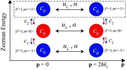
Figure 1: Schematic representation of $3\times 2$-state tunneling model for $F$=1 spinor gases. Circles represent atoms with momentum $\mathbf{p}$ in the $|F=1,m\rangle$ states. States with different $\mathbf{p}$ but the same $m$ are coupled by a moving lattice, while states with different $m$ are coupled by spin-changing interactions $c_{2}$.

Nonlinear multi-state tunneling has been primarily studied theoretically wang2006landau ; fai2015multi ; Sinitsyn_2017 ; kam2023analytical . This paper reports an experimental observation of non-exponential tunneling and dynamic self-trapping in a multi-state system realized by sodium spinor BECs with multiple spin components in one-dimensional (1D) moving lattices. We demonstrate that the tunneling process in sodium spinor BECs strongly depends on the nonlinearity induced by binary atomic interactions, and find the process is resolvable over a broader dynamic energy scale than in prior experiments with rubidium scalar BECs guan2020nonexponential . Another interesting observation is that the tunneling process in spinor gases is not always intertwined with the dynamics of the spin degree of freedom, being spin independent for a range of conditions. This is despite the fact that appreciable spin dynamics appear simultaneously throughout the tunneling process. These observations are well described by mean-field Gross-Pitaevskii (GP) simulations. Our work establishes spinor BECs as a new platform for studying nonlinear multi-state tunneling dynamics and related dynamical phase transitions in nonlinear mean-field models Smerzi1997selftrapping ; Hazzard_2021 ; marino2022dynamical .

We develop a six-state $c$-number tunneling model to provide a conceptual framework for the tunneling physics including the spin degree of freedom. The six discrete states of our $F=1$ spinor BECs are illustrated in Fig. 1, wherein each spin component exhibits tunneling between $\mathbf{p}=0$ and $\mathbf{p}=2\hbar\mathbf{k}_{L}$ momentum states coupled by the moving lattice of depth $u_{L}$ and speed $v$ changed at a ramp rate $\alpha$ while the three spin components are simultaneously coupled by spin-dependent interaction $c_{2}$. Here $\mathbf{k}_{L}$ is the lattice wave vector and $\hbar$ is the reduced Planck constant. Spin-conserving interactions $c_{0}$ and spin-changing interactions $c_{2}$ both contribute to nonlinear effects in the tunneling, with the contribution of the former being—for some atomic species such as sodium and rubidium—notably larger than the latter. The spin degree of freedom, characterized by $c_{2}$, can be thought of as introducing a distinct second dimension that leads to an enlargement of the Hilbert space from $2$ dimensions in a spinless system (see the two states encircled by the dashed box in Fig. 1) to $(2F+1)\times 2$ dimensions in a spin-$F$ spinor system. Our six-state $c$-number model shows that the tunneling process in spinor BECs is fundamentally different from the tunneling of single-component BECs even in the approximate scenario where corrections due to spin-dependent interactions are neglected. This six-state model can be reduced in some specific circumstances to an effective two-state $c$-number model.

The remainder of this paper is structured as follows. Sec. II introduces the experimental platform and observations along with comparisons to standard mean-field GP simulations. Sec. III introduces the theoretical description of tunneling in a multi-state system incorporating spatial and spin degrees of freedom, which is used to conceptually interpret our experimental observations. Finally, Sec. IV discusses applications of the multi-state tunneling dynamics, for example on the control and coupling of spin and spatial degrees of freedom.

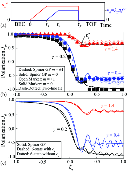
Figure 2: (a) Red (blue) lines show the experimental ramp sequence for the lattice depth $u_{L}(t)$ (the lattice speed $v(t)$). The lattice reaches its maximal depth $u_{L}^{F}$ at $t_{1}$ while reaching its maximum speed $v_{0}=\lambda_{L}\Delta f^{F}$ at $t_{2}$. (b) Solid (open) markers show experimental $J_{m}$ versus the normalized ramp time $t_{\tau}$ for the $|F=1,m=0\rangle$ ($|F=1,m=\pm 1\rangle$) states at three different $u_{L}^{F}$ and nonlinearities $\gamma$ with $\alpha=4.5E_{R}/{\rm ms}$ and $t_{F}=t_{2}$: $u_{L}^{F}=0.3E_{R}$ corresponds to $\gamma=1.4$ with $t_{\tau}^{*}=0.2$ (red), $u_{L}^{F}=1.2E_{R}$ corresponds to $\gamma=0.4$ with $t_{\tau}^{*}=0.1$ (blue), and $u_{L}^{F}=2.3E_{R}$ corresponds to $\gamma=0.2$ with $t_{\tau}^{*}=0.3$ (black). Here $t_{\tau}^{*}$ is extracted via the intersection of a piece-wise linear fit to the experimental data, as shown by the dash-dotted line for the data at $m=0$ and $\gamma=1.4$. Solid and dashed lines show spinor GP results for the $m=0$ and $m=\pm 1$ components respectively. (c) Dotted (dashed) lines show $J_{0}$ derived from the six-state $c$-number model with $c_{2}=0$ ($c_{2}=0.036c_{0}$ for our sodium system chen2019quantum ). These two lines are indistinguishable on the scale shown. Solid lines replot the $m=0$ spinor GP results from panel (b).

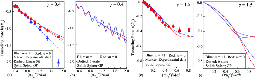
Figure 3: (a) Red (blue) color marks spin-resolved tunneling rates $\ln(R_{m})$ for the $|F=1,m=0\rangle$ ($|F=1,m=\pm 1\rangle$) states versus the normalized inverse ramp rate $x=(\pi u_{L}^{F})^{2}/(4\alpha h)$ for $t_{F}=t_{2}$ at $u_{L}^{F}=1.2E_{R}$ corresponding to $\gamma=0.4$ after sequences of variable ramp rates $6.1E_{R}/\mathrm{ms}\leq\alpha\leq 30.3E_{R}/\mathrm{ms}$ (scanned by setting $\Delta f^{F}=9.3E_{R}/h$) terminating at $t_{\tau}\gg t_{\tau}^{*}$. Markers represent the experimental $\ln(R_{m})$, which are fit by linear functions (see the dashed lines). Solid lines show 2D spinor GP simulation results. (b) Solid (dotted) lines represent spinor GP (six-state model) results for the experimental conditions shown in panel (a). (c) Similar to panel (a), except with $u_{L}^{F}=0.3E_{R}$ corresponding to $\gamma=1.5$ after sequences of variable rates $1.2E_{R}/\mathrm{ms}\leq\alpha\leq 30.3E_{R}/\mathrm{ms}$ (scanned by setting $\Delta f^{F}=4.6E_{R}/h$) terminating at $t_{\tau}=0.2$ (which is approximately equal to $t_{\tau}^{*}$ for the ramp shown in Fig. 2(b) for a similar value of $\gamma$, see also Appendix D). (d) Solid (dotted) lines represent spinor GP (six-state model) results for the experimental conditions shown in panel (c).

II Experimental results

We construct a 1D moving optical lattice with two nearly orthogonal beams of time-dependent absolute frequency difference $\Delta f(t)$ at wavelength $\lambda_{L}=1064\,$nm. The lattice has a speed $v(t)=\lambda_{L}\Delta f(t)$, a depth $u_{L}(t)$, and a potential $V_{\rm lat}(\mathbf{r},t)=u_{L}(t)\cos^{2}[\mathbf{k}_{L}\cdot\mathbf{r}-2\pi t\Delta f(t)/4]$. In this work, the recoil energy $E_{R}=h\times 3.3$ kHz is much larger than the energy scales of our optical dipole trap (ODT), the mean-field interactions, and the quadratic Zeeman shift $q=h\times 42$ Hz (see Table 1 in Appendix C). Here $h$ is Planck’s constant.

Similar to our previous work chen2019quantum ; zhao2014dynamics ; zhao2015antiferromagnetic ; 2023dSMA ; austin2021pra ; austin2021quantum , the experimental sequences begin with a $F=1$ spinor BEC of up to $N=1.0\times 10^{5}$ sodium atoms in an ODT with angular frequencies $\omega_{x,y,z}=2\pi\times(120,120,160)$ Hz. We apply resonant radio-frequency pulses to prepare an initial state with fractional population $\rho_{0}\approx 0.5$ in the $|F=1,m=0\rangle$ state and $\rho_{\pm 1}\approx 0.25$ in the $|F=1,m=\pm 1\rangle$ states. We then adiabatically load atoms into the lattice via a sequence shown in Fig. 2(a). For $t\leq t_{1}$, the depth $u_{L}$ is increased linearly from 0 to $u_{L}^{F}$ while $\Delta f$ remains at 0 (i.e., lattices are stationary). For $t_{1}\leq t\leq t_{2}$, while keeping $u_{L}(t)$ at $u_{L}^{F}$, we set the tunneling control parameter $\delta(t)=-4E_{R}+\alpha t$ by linearly ramping $\Delta f$ at a rate $\alpha=\dfrac{h(\Delta f(t_{2})-\Delta f(t_{1}))}{t_{2}-t_{1}}$ such that $\Delta f$ reaches its final value $\Delta f^{F}$ at $t=t_{2}$. Here $4E_{R}$ is the kinetic energy difference of the $\mathbf{p}=0$ and $\mathbf{p}=2\hbar\mathbf{k}_{L}$ momentum states.

In the absence of interactions, a fully adiabatic ramp of $\Delta f$ from $0$ to $8E_{R}/h$ transfers atoms in the initial $\mathbf{p}=0$ state to the final $\mathbf{p}=2\hbar\mathbf{k}_{L}$ state. The effective coupling between these two momentum states is maximal halfway through the ramp where $\Delta f=4E_{R}/h$ and $\delta=0$. At $t=t_{F}$, we abruptly switch off the lattice and ODT and let atoms ballistically expand for a certain time of flight (TOF) before monitoring them via two-step microwave imaging 2023dSMA ; chen2019quantum .

To study tunneling dynamics in the multi-state system possessing spin and spatial degrees of freedom, we experimentally monitor the spin-resolved polarizations

$$J_{m}=\frac{N_{m,\mathbf{p}=0}-N_{m,\mathbf{p}\neq 0}}{N_{m,\mathbf{p}=0}+N_{m,\mathbf{p}\neq 0}}~{}.$$ (1)

Here $N_{m,\mathbf{p}=0}$ ($N_{m,\mathbf{p}\neq 0}$) denotes the number of atoms with zero (nonzero) momentum in the $|F=1,m\rangle$ state. Our data indicate that the measured $N_{m,\mathbf{p}\neq 0}$ are dominated by the $\mathbf{p}=2\hbar\mathbf{k}_{L}$ contribution.

Figure 2(b) shows measured polarizations $J_{m}$ of $|F=1,m\rangle$ spin components versus the normalized ramp time $t_{\tau}=\dfrac{\alpha(t_{2}-t_{1})}{4E_{R}}-1$ for a constant rate $\alpha=4.5E_{R}/{\rm ms}$ at various experimental conditions. The experimental data at each condition demonstrate that $J_{m}$ are very close to $1$ for negative $t_{\tau}$, change rapidly in a narrow transition region around $t_{\tau}=0$ (where the $\mathbf{p}=0$ and $\mathbf{p}=2\hbar\mathbf{k}_{L}$ states are coupled maximally), and become approximately constant for positive $t_{\tau}$. We therefore can extract a critical normalized ramp time $t_{\tau}^{*}$, via the intersection of a piece-wise linear function as illustrated by the dash-dotted line in Fig. 2(b), that demarcates the end of the transition region from the final equilibration region in which momentum state populations plateau. Interestingly, our experimental data indicate that the observed transition regions at various experimental conditions are narrower (i.e., have smaller $t_{\tau}^{*}$) than those observed previously in a rubidium system guan2020nonexponential . This is ascribed to the energy scales intrinsic to the system, i.e., the larger recoil energy (see Appendix C). Typical experimental examples are shown in Fig. 2(b) for three different dimensionless spin-independent nonlinearities $\gamma=2c_{0}/u_{L}$ wu2000nonlinear ; guan2020nonexponential . This definition of $\gamma$ ignores spin-dependent corrections as $c_{2}=0.036c_{0}\ll c_{0}$ in our sodium system chen2019quantum , and enables direct comparisons with the nonlinear two-state model and prior experiments on scalar BECs guan2020nonexponential . The dependence of the tunneling process on $\gamma$ is rather pronounced. For example, at $\gamma=0.2$ the lattice coupling dominates and the tunneling is spin independent resulting in the majority of the population residing in the $\mathbf{p}=0$ ($\mathbf{p}=2\hbar\mathbf{k}_{L}$) state or $J_{m}=1$ ($J_{m}=-1$) at $t_{\tau}=-1$ ($t_{\tau}\geq t_{\tau}^{*}$). However, for $\gamma=0.4$ and $1.4$ the nonlinearity has a truly non-perturbative effect with a significant fraction of atoms remaining in the $\mathbf{p}=0$ state at the end of the ramp, i.e., the observed $J_{m}$ at $t_{\tau}\geq t_{\tau}^{*}$ plateau at a value larger than $-1$. Such residual $\mathbf{p}=0$ populations are consistent with non-vanishing tunneling between the asymptotically decoupled eigenstates and, for $\gamma=1.4$ self-trapping due to the presence of swallow-tails in the adiabatic or instantaneous energy spectrum might be at play guan2020nonexponential ; wu2000nonlinear ; choi_1999 . Typically for $t_{\tau}<t_{\tau}^{*}$ differences between $J_{0}$ and $J_{\pm 1}$ are small. However for $t_{\tau}>t_{\tau}^{*}$, we observe statistically significant spin dependent behavior, e.g., differences between $J_{0}$ and $J_{\pm 1}$ curves in Fig. 2(b) for $\gamma=0.4$. We also conduct parameter-free numerical simulations with the time-dependent mean-field spinor GP equation using a reduced $2$D geometry (see Appendix A) and find theory-experiment agreement (see Fig. 2(b)), indicating the spinor dynamics is, as expected, in the mean-field regime with negligible quantum and thermal effects.

We repeat the experiments for various ramp rates $\alpha$ and plot the measured spin-resolved tunneling rates,

$$\ln(R_{m})=\ln\left(\frac{N_{m,\mathbf{p}=0}}{N_{m,\mathbf{p}=0}+N_{m,\mathbf{p}\neq 0}}\right),$$ (2)

as a function of the dimensionless inverse ramp rate $x=(\pi u_{L}^{F})^{2}/(4\alpha h)$ for two values of $\gamma$ in Fig. 3. The variable $x$ is chosen since $\ln(R_{m}(t))$ depends linearly on $x$ in the linear LZ two-state model khomeriki2010nonlinear ; zhang2019nonlinear ; guan2020nonexponential . In Fig. 3(a), $\gamma=0.4$ and the tunneling rate is extracted at $t_{\tau}=1.3\gg t_{\tau}^{*}$. The experimental tunneling rates agree with a linear fit (dashed lines in Fig. 3(a)) for $x\lesssim 1.4$ indicating exponential tunneling in this region. The experimental results for the $|F=1,m=0\rangle$ component are also nicely reproduced by spinor GP simulations (solid lines in Fig. 3), which include the density-dependent and spin-dependent interaction coefficients. Interestingly, a splitting occurs in the tunneling rates between the $|F=1,m=0\rangle$ and $|F=1,m=\pm 1\rangle$ spin components at $x>1$. A qualitatively similar but notably smaller splitting is also predicted by the GP simulations. Discrepancies with the experimental observations for the $|F=1,m=\pm 1\rangle$ component could be attributed to limitations of our theoretical model, such as the reduced $2$D simulation geometry. In contrast, the data in Fig. 3(c), taken at a large nonlinearity ($\gamma=1.5$) and $t_{\tau}\approx t_{\tau}^{*}$, clearly shows evidence of interaction induced non-exponential behavior in the tunneling process guan2020nonexponential . Another key finding from Fig. 3(c) is that the observed tunneling process is spin independent. This result, when combined with the spin-dependent behavior observed in Fig. 3(a), indicates a spin-dependent multi-state tunneling process that collapses into a spin-independent process under certain conditions, such as $t_{\tau}<t_{\tau}^{*}$ or large $\alpha$ such as $(\pi u_{L}^{F})^{2}/(4\alpha h)<1$ for $\gamma=0.4$ in Fig. 3(a) and $\gamma=1.5$ in Fig. 3(c). General conditions for spin-dependent tunneling related to the timescales of the system are elucidated further in Sec. III.

Figure 4 displays the time evolution of $\rho_{0,0}$, the fractional population of atoms with zero momentum in the $|F=1,m=0\rangle$ state, demonstrating that appreciable spin dynamics occur alongside the tunneling process for three different ramp sequences with similar nonlinearities ($\gamma>1$): black diamonds (blue circles) represent spin oscillations extracted from experimental data shown in Fig. 2(b) (Fig. 3(c)), while red triangles represent observations after an infinitely fast ramp, i.e., a quench with the ramp rate of $\alpha=\infty$. The apparent agreement in spin dynamics between the three curves in Fig. 4 is strikingly at odds with the observation of spin-dependent tunnelling dynamics only at large moving lattice speeds and small $\alpha$ in Figs. 2(b) and 3(a). To reconcile these seemingly contradictory observations, Sec. III introduces a six-state model that provides a rigorous framework for interpreting the experimental results.

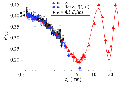
Figure 4: Experimental time evolution of the fractional spin population $\rho_{0,0}$ at $u_{L}^{F}=0.3E_{R}$ for three different ramp sequences with similar nonlinearities: a sequence with a fixed finite $\alpha$ and $t_{2}=t_{F}$ (black; extracted from red curves in Fig. 2(b)), a sequence with varying $\alpha$ such that $\Delta f^{F}=4.6E_{R}/h$ at $t_{2}=t_{F}$ (blue; extracted from experimental data shown in Fig. 3(c)), and a quench sequence with $\alpha=\infty$ (red; $\Delta f^{F}=4.6E_{R}/h$). The solid line is a sine fit to the red data for guiding the eye.

III Six-state $c$-number model

As shown in Section II, the experimental results are overall well captured by the mean-field spinor GP equation, which accounts for both density-dependent and spin-dependent interactions. Within this mean-field description (see Appendix A for details), the dynamics are governed by $2F+1$ mean-field spinor components $\psi_{m}(\mathbf{r},t)$ that depend on the spatial coordinate $\mathbf{r}$ and time $t$. These spin components are normalized such that $\sum_{m=0,\pm 1}\int|\psi_{m}(\mathbf{r},t)|^{2}d\mathbf{r}=1$. This section starts with the spinor GP equation and derives from it a six-state $c$-number model, providing a theoretical framework to interpret the observed tunneling dynamics and to reconcile the observations of Figs. 2-4.

We start our derivation by introducing an ansatz for the spatially and time-dependent mean-field wavefunction of each spinor component,

$$\psi_{m}(\mathbf{r},t)=\phi_{m,0}(\mathbf{r},t)+\phi_{m,2}(\mathbf{r},t)e^{2\imath\mathbf{k}_{L}\cdot\mathbf{r}}.$$ (3)

This ansatz generalizes earlier work for the single-component BECs guan2020nonexponential ; guan2020Rabi . Since the experiment populates predominantly two distinct momentum states $\mathbf{p}=0$ and $\mathbf{p}=2\hbar\mathbf{k}_{L}$, the ansatz accounts only for these momentum components. Consistent with the fact that the momentum width of the initial BEC is small compared to $\hbar k_{L}$, we assume

$$\int\left[\phi_{m,0}(\mathbf{r},t)\right]^{*}\phi_{m,2}(\mathbf{r},t)e^{2\imath\mathbf{k}_{L}\cdot\mathbf{r}}~{}d\mathbf{r}=0.$$ (4)

Inserting Eq. (3) into the spinor GP equation (see Appendix B), with the assumption that $\phi_{m,k}(\mathbf{r},t)$ with $k=0$ and $2$ follow a Thomas-Fermi profile and the ODT can be neglected during the ramp protocol, the spatial dependence can be integrated out to obtain an effective time-dependent Schrödinger equation,

$$\imath\hbar\partial_{t}\mathbf{d}(t)={H}^{(6)}\mathbf{d}(t),$$ (5)

where $\partial_{t}$ denotes the derivative with respect to time. In Eq. (5), $\mathbf{d}(t)=(d_{-1,0},d_{-1,2},d_{0,0},d_{0,2},d_{+1,0},d_{+1,2})^{T}$ is the state vector that collects the $c$-numbers $d_{m,k}(t)$, which correspond to the $m=0,\pm 1$ Zeeman and $k=0,2$ momentum components, respectively. We employ the state normalization $\sum_{m,k}|d_{m,k}(t)|^{2}=1$. Since the experiment predominantly occupies the $\mathbf{p}=0$ and $2\hbar\mathbf{k}_{L}$ components, the experimentally measured atom numbers $N_{m,\mathbf{p}\neq 0}$ can be compared directly with the six-state model populations $N|d_{m,2}|^{2}$.

The six-state $c$-number Hamiltonian ${H}^{(6)}$ can be divided into two pieces, ${H}^{(6)}={H}^{(6,D)}+{H}^{(6,S)}$. The Hamiltonian ${H}^{(6,D)}$ accounts for the optical lattice, the density-dependent (and spin-independent) interactions, and the quadratic Zeeman energy $q$. The Hamiltonian ${H}^{(6,S)}$ accounts for the spin-dependent interactions. The energy scale of $H^{(6,S)}$ is set by the spin-dependent interaction coefficient $c_{2}=g_{2}n_{\text{mean}}$, where $g_{2}$ denotes the spin-dependent interaction coefficient (see Appendix A) and $n_{\text{mean}}$ the mean density.

The Hamiltonian ${H}^{(6,D)}(t)$ has the following block diagonal structure:

$${H}^{(6,D)}(t)=\begin{pmatrix}{H}^{(2)}_{-1}(t)&{0}&{0}\\ {0}&{H}^{(2)}_{0}(t)&{0}\\ {0}&{0}&{H}^{(2)}_{+1}(t)\end{pmatrix},$$ (6)

where the $2\times 2$ blocks ${H}^{(2)}_{m}(t)$ on the diagonal are given by

$${H}^{(2)}_{m}(t)=\frac{1}{2}\begin{pmatrix}\delta(t)+2|m|q&\frac{u_{L}^{F}}{2}+2A(\mathbf{d},t)\\ \frac{u_{L}^{F}}{2}+2A^{*}(\mathbf{d},t)&-\delta(t)+2|m|q\end{pmatrix}.$$ (7)

The control parameter $\delta(t)=-4E_{R}+\alpha t$ arises, as in the non-linear two-state $c$-number model for a scalar BEC (see Ref. guan2020nonexponential ), from the kinetic energy difference of the two coupled momentum states and the fact that the lattice is moving. The additional $|m|q$ terms on the diagonal are due to the quadratic Zeeman shift. The quantity

$$A(\mathbf{d},t)={c}_{0}\sum_{m=\pm 1,0}(d_{m,2}(t))^{*}d_{m,0}(t)$$ (8)

denotes the nonlinearity that is associated with the spin-independent interactions; here, $c_{0}=g_{0}n_{\text{mean}}$ (see Appendix A). Note that $A(\mathbf{d},t)$ appears on the off-diagonals as opposed to the diagonals as in the widely studied non-linear two-state model wu2000nonlinear ; liu2002theory ; zhang2019nonlinear ; trimborn2010nonlinear ; khomeriki2010nonlinear ; guo2016nonlinear (see below for further discussion). To interpret the six-state $c$-number Hamiltonian, we first assume that $c_{2}$, which is about $28$ times smaller than $c_{0}$ for sodium chen2019quantum , can be set to zero, i.e., we neglect the contribution of $H^{(6,S)}$. This assumption is, as confirmed by numerical simulations (see Fig. 2(c) and discussion below), well justified.

The Hamiltonian ${H}^{(6,D)}(t)$ has the following characteristics. (i) Even though the apparent block-diagonal structure suggests that it decouples into three independent $2\times 2$ blocks (i.e., a set of independent two-state models each associated with a single Zeeman component), this is not, in general, the case since the evaluation of $A(\mathbf{d},t)$ requires—as indicated by the $\mathbf{d}$ argument—knowledge of the coefficients $d_{m,k}(t)$ of all three Zeeman components. Even when ${H}^{(6,S)}$ is neglected, the description of tunneling in spin-1 BECs requires, in general, a six-state model. (ii) Importantly, the nonlinearity $A(\mathbf{d},t)$ is the same in each $m$-subspace, i.e., the tunneling dynamics in the different $m$ channels is governed by the same nonlinearity. (iii) The nonlinearity $A(\mathbf{d},t)$ in general depends on the coherences (i.e., relative phases of the state vector elements) and not just on population differences. Properties (i)-(iii) make the tunneling of spinor BECs in a moving optical lattice fundamentally different from tunneling of single-component BECs in a moving optical lattice even in the approximate scenario where corrections due to the spin-dependent interactions are neglected (i.e., in the case where $c_{2}$ is set to zero). Property (ii) also provides an explanation as to why the experimental and spinor GP tunneling data in Figs. 2(b) and 3(c) are, for a good number of parameter combinations and times, approximately independent of $m$. Since the nonlinearity on the off-diagonals of $H^{(6,D)}$ is the same in each $m$ subspace, the spin dependence of the tunneling dynamics should be small for certain conditions.

We now formally show that the six-state c-number model reduces for specific conditions, which are fulfilled to varying degrees in our experiment, to an effective two-state model that neglects the spin degrees of freedom. If we define new coefficients $b_{k}(t)$ through

$${b}_{k}(t)=\sqrt{\frac{1}{|d_{m,0}|^{2}+|d_{m,2}|^{2}}}d_{m,k}(t),$$ (9)

then the coefficients $b_{k}(t)$ are, for each $m$, except for an overall phase that does not impact the populations, governed by the time-dependent two-state Schrödinger equation $\imath\hbar\partial_{t}\mathbf{b}(t)={H}^{(2)}(t)\mathbf{b}(t)$ with state vector $\mathbf{b}(t)=(b_{0}(t),b_{2}(t))^{T}$ and Hamiltonian $H^{(2)}(t)$,

$${H}^{(2)}(t)=\frac{1}{2}\left(\begin{array}[]{cc}\delta(t)-c_{0}\Delta b(t)&u_{L}^{F}/2\\ u_{L}^{F}/2&-\delta(t)+c_{0}\Delta b(t)\end{array}\right).$$ (12)

Equation (12) reveals that the single-particle term $\delta(t)$ is accompanied by a nonlinear detuning $c_{0}\Delta b(t)$, which depends on the population difference $\Delta b(t)=|b_{0}(t)|^{2}-|b_{2}(t)|^{2}$. This nonlinear detuning is obtained by rewriting the original $A(\mathbf{d},t)$ term of the six-state model. Thus, provided Eq. (9) holds, the six-state model with ${H}^{(6,S)}$ set to zero formally decouples into three independent, identical two-state models, i.e., the equations of motion and associated evolution for each Zeeman component are identical up to a scaling factor that is associated with the (conserved) fractional population of each Zeeman component. The Hamiltonian $H^{(2)}(t)$ is the celebrated non-linear two-state $c$-number Landau-Zener Hamiltonian wu2000nonlinear ; liu2002theory ; zhang2019nonlinear ; trimborn2010nonlinear ; khomeriki2010nonlinear ; guo2016nonlinear , which was experimentally realized in Ref. guan2020nonexponential using rubidium.

The inclusion of the Hamiltonian ${H}^{(6,S)}$ leads to an explicit coupling between the different $m$ channels, thereby invalidating the above mapping to three independent $2\times 2$ Hamiltonians. However, the coupling is negligible for a large fraction of the parameter combinations considered in Figs. 2 and 3. The reasons are: First, $c_{2}$ is much smaller than $c_{0}$. Second, the length of the ramps is, in many cases, sufficiently short such that $c_{2}(t_{2}-t_{1})/h$ is negligibly small. Third, the experimentally prepared initial state has no phase difference between the spin components (see Appendix E). In what follows, we use the six- and two-state c-number models to further interpret the experimental data and spinor GP results shown in Figs. 2(b), 3(a), and 3(c).

For the ramps shown in Fig. 2(c), we note the following key observations regarding the six-state model. (i) For each of the three nonlinearities $\gamma$ considered ($\gamma=0.2,0.4$ and $1.4$), the polarization $J_{0}$ obtained from the six-state $c$-number model with finite $c_{2}$ (dashed lines) and with $c_{2}$ artificially set to zero (dotted lines) are essentially identical. (ii) The polarizations $J_{\pm 1}$ for the $m=\pm 1$ components (not plotted) are essentially identical to the $J_{0}$ result shown. These two observations indicate that, within the $c$-number model, the spin-mixing interactions of strength $c_{2}$ have a negligible impact on the tunneling populations for the ramps studied in Fig. 2(c) (specifically, using $\alpha=4.5E_{R}/$ms). Since the six-state c-number model reduces, for $c_{2}=0$ and the initial conditions considered in the experiment, to an effective two-state model (see above), the agreement between the six-state models with $c_{2}\neq 0$ and $c_{2}=0$ shows that the dependence of $J_{m}$ on $\gamma$ is consistent with what has been observed for a single-component BEC guan2020nonexponential .

Next, we compare the results shown in Fig. 2(c) for the six-state model (dashed and dotted lines) and the spinor GP simulations (solid lines). (i) While the overall agreement between the two theories is quite good, the six-state model predicts larger amplitude oscillations for $t_{\tau}>0$ than the spinor GP simulations. These oscillations are a consequence of the finite ramp window, i.e., the fact that the states are not fully decoupled at $t_{\tau}=1$ guan2020nonexponential ; cao2020probing . In-trap dynamics, which is captured by the spinor GP equation but not by the $c$-number Hamiltonian, washes these oscillations out. (ii) For all three $\gamma$ values considered, the polarizations obtained from the six-state model lie slightly above those obtained from the spinor GP simulations in the transition region, where $J_{0}$ changes rapidly with increasing $t_{\tau}$. For example, focusing on the $\gamma=0.2$ case (black lines), the polarization $J_{0}$ obtained from the GP simulations (solid black line) reaches negative values slightly earlier (around $t_{\tau}\approx-0.05$) than those obtained from the six-state model (dashed black line). This small discrepancy is attributable to the broadening of the resonance condition – i.e., where the two momentum components are maximally coupled – in the spinor GP framework as a result of the finite momentum width or, equivalently, the inhomogeneous spatial density profile of the condensate.

The dotted lines in Figs. 3(b) and 3(d) show the six-state model tunneling rates $\ln(R_{m})$ for $\gamma=0.4$ and $\gamma=1.5$, respectively, as a function of the dimensionless inverse ramp rate $(\pi u_{L}^{F})^{2}/(4\alpha h)$ for the same parameters as used in Figs. 3(a) and 3(c). Figure 3(b) shows reasonably good quantitative agreement between the six-state (dotted lines) and GP (solid lines) results for “fast” ramps, i.e., $(\pi u_{L}^{F})^{2}/(4\alpha h)\lesssim 0.8$ (here “fast” refers to ramp sequences in absolute units (ms) that are comparatively short, see also Appendix E). Consistent with the spin independence of the polarizations $J_{m}$ as discussed in the context of Fig. 2(c), the tunneling rates obtained using the two theories are approximately spin-independent ($m=\pm 1$ data are shown as blue lines and $m=0$ data as red lines) for “fast” ramps. However, for “slower” ramps, $(\pi u_{L}^{F})^{2}/(4\alpha h)\gtrsim 0.8$, the $c$-number model and spinor GP results deviate for primarily two reasons. First, the $c$-number model displays large oscillations that are centered approximately around the spinor GP predictions. These arise, as discussed previously, due to the finite ramp window and are washed out in the GP model due to in-trap dynamics for which the timescale is set by the spin-independent interactions of strength $c_{0}$ and the ODT. These are not accounted for in the $c$-number model. Second, while the $c$-number model predicts slightly spin dependent tunneling rates for $(\pi u_{L}^{F})^{2}/(4\alpha h)\gtrsim 1.5$, the spinor GP framework yields a stronger splitting between the $m=0$ and $m=\pm 1$ observables beginning from about $(\pi u_{L}^{F})^{2}/(4\alpha h)\gtrsim 1.3$. From the perspective of the six-state model, the emergence of spin dependent observables can be understood from the fact that data in this range correspond to a $c_{2}(t_{2}-t_{1})/h$ which is no longer completely negligible (see also Appendix E). This emphasizes that, even though $c_{2}/c_{0}$ is small, spin dependent processes can play a role in the observed tunneling dynamics. We interpret the fact that the deviation between $\ln(R_{0})$ and $\ln(R_{\pm 1})$ is notably larger for the spinor GP than the $c$-number results as an indicator that the precise details of the spatial dynamics of the BEC become increasingly more important as the ramp duration increases.

Comparing the $c$-number and GP predictions for $\gamma=1.5$, Fig. 3(d) shows trends similar to those observed for $\gamma=0.4$. However, as the tunneling rates are obtained much closer, at $t_{\tau}\approx t_{\tau}^{*}$, to the region of maximal effective coupling, the discrepancies between the spinor GP and six-state $c$-number models are amplified. In particular, the previously mentioned oscillations, which are a feature of the $c$-number model for finite ramp windows, are primarily responsible for the deviations between the models, which start to emerge for $(\pi u_{L}^{F})^{2}/(4\alpha h)\approx 0.2$ and become increasingly larger as $(\pi u_{L}^{F})^{2}/(4\alpha h)$ increases.

IV Conclusion

We have observed non-exponential tunneling and dynamic self-trapping in $F=1$ spinor BECs that realize a six-state $c$-number tunneling model. Our data have demonstrated that the tunneling dynamics strongly depend on the nonlinearity induced by interactions and are resolvable over a broader dynamic energy scale than in prior experiments with rubidium scalar BECs guan2020nonexponential . We have also found the tunneling process is influenced by the spin degree of freedom under certain conditions. Our work opens up exciting prospects for alternative multi-state ramps and state transfer protocols, including studies aimed at coupling the spatial and spin degrees of freedom. In addition, we have introduced spinor BECs as a simulator of nonlinear multi-state quantum tunneling Hamiltonians, by utilizing the magnetic or spin degree of freedom to enlarge the Hilbert space.

The ramps utilized in this work complement earlier sodium spinor BEC studies 2023dSMA , in which the moving one-dimensional optical lattice was quenched. While the quench triggered significant spatial dynamics, including fracturing of the BEC, the spatial dynamics did not destroy the coherent spin dynamics. Together with our current work, these studies suggest that the dynamical coupling of the spatial and spin degrees of freedom may be exploited to produce effective two or multi-state tunneling systems dependent upon the choice of initial conditions.

Appendix A Gross-Pitaevskii model of spinor BEC

At the mean-field level, the dynamics of a weakly-interacting $F$=1 spinor BEC subject to a time-dependent potential $V(\mathbf{r},t)$ is modeled by the time-dependent three-component or spinor GP equation ueda2012review ; stamper2013spinor ,

$$i\hbar\frac{\partial}{\partial t}\begin{pmatrix}\psi_{-1}\\ \psi_{0}\\ \psi_{1}\end{pmatrix} =\left[-\frac{\hbar^{2}\nabla^{2}}{2M_{\rm Na}}+V(\mathbf{r},t)+g_{0}(N-1)\left(|\psi_{-1}|^{2}+|\psi_{0}|^{2}+|\psi_{1}|^{2}\right)\right]\begin{pmatrix}\psi_{-1}\\ \psi_{0}\\ \psi_{1}\end{pmatrix}+\begin{pmatrix}q&0&0\\ 0&0&0\\ 0&0&q\end{pmatrix}\begin{pmatrix}\psi_{-1}\\ \psi_{0}\\ \psi_{1}\end{pmatrix}$$

$$+g_{2}(N-1)\begin{pmatrix}|\psi_{-1}|^{2}+|\psi_{0}|^{2}-|\psi_{1}|^{2}&\psi_{1}^{*}\psi_{0}&0\\ \psi_{1}\psi_{0}^{*}&|\psi_{1}|^{2}+|\psi_{-1}|^{2}&\psi_{-1}\psi_{0}^{*}\\ 0&\psi_{-1}^{*}\psi_{0}&|\psi_{1}|^{2}+|\psi_{0}|^{2}-|\psi_{-1}|^{2}\end{pmatrix}\begin{pmatrix}\psi_{-1}\\ \psi_{0}\\ \psi_{1}\end{pmatrix}.$$

Here, $\psi_{m}(\mathbf{r},t)$ is the mean-field GP wavefunction that is associated with the Zeeman component $m$ ($m=0,\pm 1$) and $M_{\text{Na}}$ denotes the mass of a ²³Na atom. The two-body interactions are split into a pair of distinct contributions: density-density (i.e., spin-independent) collisions are characterized by the interaction coefficient $g_{0}$, while spin-dependent collisions are characterized by the coefficient $g_{2}$. The coupling constants $g_{0}$ and $g_{2}$ are given by $4\pi\hbar^{2}/M_{\text{Na}}$, multiplied by the corresponding scattering lengths. Specifically,

$$\begin{gathered}g_{0}=\frac{4\pi\hbar^{2}(a_{S=0}+2a_{S=2})}{3M_{\rm Na}},\\ g_{2}=\frac{4\pi\hbar^{2}(a_{S=2}-a_{S=0})}{3M_{\rm Na}},\end{gathered}$$ (14)

where $a_{S=0}=48.9a_{0}$ ($a_{S=2}=54.5a_{0}$) are the $s$-wave scattering lengths for the $F=0$ ($F=2$) states ($a_{0}$ is the Bohr radius) Knoop2011PRA ; chen2019quantum . The external potential $V(\mathbf{r},t)$ contains the lattice potential $V_{\text{lat}}(\mathbf{r},t)$ as well as the approximately harmonic ODT (see Sec. II). For the experiments discussed in this paper, the initial $n_{\text{mean}}$ is up to $6\times 10^{19}~{}\mathrm{m}^{-3}$.

The spinor GP simulation data shown in Figs. 2(b), 2(c), and 3 are for $N=10^{5}$ atoms. We exploit the axial symmetry of the experimental system ($\omega_{x}=\omega_{y}$) and construct, following the procedure discussed in Ref. 2023dSMA , an effective $2$D system that accounts for the ODT, moving lattice, and gravity. The initial state preparation mimics what is done in the experiment. We first equilibrate a single-component BEC in the absence of the lattice, then “redistribute” population so that the $m=-1$, $0$, and $+1$ states have fractional populations of $1/4$, $1/2$, and $1/4$, respectively, and finally ramp the lattice with $\Delta f=0$ to its desired value $u_{L}^{F}$ at a rate $1.6$ $E_{R}/$ms. Our procedure assumes that the duration of the pulse that redistributes the population is infinitely short; we checked that a finite pulse length does not notably change the results.

Appendix B $c$-number model of multi-state tunneling

Section III develops a six-state $c$-number model of the tunneling dynamics in a spinor BEC subject to an optical lattice, which provides—compared to the spinor GP framework—a much simplified description of the system. In deriving ${H}^{(6)}$, we assume that the contribution from the external ODT to the spinor GP equation can be set to zero, i.e., it is assumed that the impact of the ODT on the spatial dynamics of the spinor BEC during the ramp can be neglected. While this is not strictly true, the approximation is reasonable for the lattice ramps considered in Sec. II, which last up to a few ms, corresponding to at most roughly one trap oscillation period.

The frequency difference $\Delta f(t)$ of the two moving lattice beams enters via an energy splitting between the two momentum components and takes the form,

$$\delta(t)=-4E_{R}+\pi\hbar\Delta f(t)+\pi\hbar\frac{\partial\Delta f(t)}{\partial t}t.$$ (15)

For the linear ramp $\Delta f(t)=\alpha t/h$ employed in the experiment, $\delta(t)$ reduces to the equation given in Sec. II.

The contribution $H^{(6,S)}$ to the six-state model can be written as

$$H^{(6,S)}=\begin{pmatrix}S_{0}&0\\ 0&S_{2}\end{pmatrix},$$ (16)

where the matrices $S^{(0)}$ and $S^{(2)}$ read

$$S_{0}=\begin{pmatrix}{c}_{2}(|d_{0,0}|^{2}+|d_{0,2}|^{2})&{c}_{2}(d_{0,0}d_{1,0}^{*}+d_{-1,2}d_{0,2}^{*}+2d_{0,2}d_{1,2}^{*})&0\\ {c}_{2}(d_{0,0}^{*}d_{1,0}+d_{-1,2}^{*}d_{0,2}+2d_{0,2}^{*}d_{1,2})&{c}_{2}(|d_{-1,0}|^{2}+|d_{1,0}|^{2}+|d_{-1,2}|^{2}+|d_{1,2}|^{2})&{c}_{2}(d_{-1,0}d_{0,0}^{*}+d_{0,2}d_{1,2}^{*}+2d_{-1,2}d_{0,2}^{*})\\ 0&{c}_{2}(d_{-1,0}^{*}d_{0,0}+d_{0,2}^{*}d_{1,2}+2d_{-1,2}^{*}d_{0,2})&{c}_{2}(|d_{0,0}|^{2}+|d_{0,2}|^{2})\end{pmatrix}$$

$$S_{2}=\begin{pmatrix}{c}_{2}(|d_{0,0}|^{2}+|d_{0,2}|^{2})&{c}_{2}(d_{0,2}d_{1,2}^{*}+d_{-1,0}d_{0,0}^{*}+2d_{0,0}d_{1,0}^{*})&0\\ {c}_{2}(d_{0,2}^{*}d_{1,2}+d_{-1,0}^{*}d_{0,0}+2d_{0,0}^{*}d_{1,0})&{c}_{2}(|d_{-1,0}|^{2}+|d_{1,0}|^{2}+|d_{-1,2}|^{2}+|d_{1,2}|^{2})&{c}_{2}(d_{-1,2}d_{0,2}^{*}+d_{0,0}d_{1,0}^{*}+2d_{-1,0}d_{0,0}^{*})\\ 0&{c}_{2}(d_{-1,2}^{*}d_{0,2}+d_{0,0}^{*}d_{1,0}+2d_{-1,0}^{*}d_{0,0})&{c}_{2}(|d_{0,0}|^{2}+|d_{0,2}|^{2})\end{pmatrix}.$$

The energy scale of $H^{(6,S)}$ is set by the spin-dependent interaction coefficient $c_{2}$. This implies that the contribution of $H^{(6,S)}$ is much weaker than $H^{(6,D)}$, as $c_{2}$ for sodium is about 28 times smaller than the spin-independent interaction scale $c_{0}$ Knoop2011PRA ; chen2019quantum . However, as shown by the spin dynamics in Fig. 4, we do probe time scales where the contribution from terms proportional to $c_{2}$ can, in principle, give rise to non-negligible dynamics and thus it is not a priori clear that $H^{(6,S)}$ can be neglected.

Appendix C Comments on units and parameters

The nonlinear six-state $c$-number model is characterized by five energy scales, namely the coupling strength $u_{L}^{F}/2$, the density-dependent interaction energy $c_{0}$, the recoil energy $E_{R}$ (which enters through the detuning), the quadratic Zeeman shift $q$, and the spin-dependent interaction energy $c_{2}$ (see Table 1). If we restrict ourselves to situations where the six-state $c$-number model maps cleanly to the two-state $c$-number model (see Appendices B and E), the latter two energy scales drop out of the problem: the resulting two-state $c$-number model can be written in terms of two dimensionless energy ratios, namely $\gamma=c_{0}/(u_{L}^{F}/2)$ and $(u_{L}^{F}/2)/(4E_{R})$. The dimensionless non-linearity $\gamma$ is used throughout this paper to quantify the relative strength between the density-dependent interaction $c_{0}$ and the coupling strength $u_{L}^{F}/2$, which is equal to the energy gap at zero detuning for $c_{0}=0$. The competition between the interactions and coupling are most prominent for $\gamma$ around one wu2000nonlinear ; liu2002theory ; guan2020nonexponential ; specifically, Figs. 2-3 consider $\gamma$ between $0.2$ and $1.5$.

The energy ratio $(u_{L}^{F}/2)/(4E_{R})$ compares the energy gap at zero detuning with the energy gap at the beginning of the ramp, both calculated for $c_{0}=0$. In the “ideal” nonlinear two-state Landau-Zener model wu2000nonlinear ; liu2002theory , where the detuning is varied from $-\infty$ to $\infty$, this energy ratio is equal to zero, i.e., it drops out of the problem. In experimental implementations of the non-linear Landau-Zener model, this energy ratio is finite but should be small. For our lattice based tunneling simulator results shown in Fig. 2, the ratio $(u_{L}^{F}/2)/(4E_{R})$ varies from about $0.3$ for $\gamma=0.2$ to $0.04$ for $\gamma=1.4$. The smaller this energy ratio is, the more decoupled the two states are initially. The interplay of the two energy ratios determines the width $t_{\tau}^{*}$ of the transition region, which we quantify empirically by performing piecewise linear fits (see Sec. II). It should be noted that the dimensionless transition width $t_{\tau}^{*}$ is expressed as a fraction of the total ramp time $t_{2}-t_{1}$ for a given $\alpha$. As discussed in Ref. guan2020nonexponential , the dimensionless non-linearity $\gamma$ and the dimensionless ramp time are normalized using “inconsistent” energy scales, namely $u_{L}^{F}/2$ and $\alpha(t_{2}-t_{1})$, respectively.

It was commented in the discussion surrounding Fig. 2 that the width of the transition region for our sodium tunneling simulator is narrower, if expressed in terms of the dimensionless ramp time that uses $\alpha(t_{2}-t_{1})$ (which depends on $E_{R}$) as energy unit, than that for the rubidium tunneling simulator realized by the WSU group guan2020nonexponential . This can be understood by noting that their $(u_{L}^{F}/2)/(4E_{R})$ values range from $0.88$ for $\gamma=0.306$ to $0.25$ for $\gamma=1.07$. The roughly $2.5$ times larger value of $(u_{L}^{F}/2)/(4E_{R})$ in the rubidium realization compared to our sodium realization is due to the about three times larger recoil energy for the sodium than the rubidium experiment. As a consequence, the sodium realization is closer to the ideal non-linear Landau-Zener model that is characterized by $(u_{L}^{F}/2)/(4E_{R})=0$.

Parameter	Energy/$h$	Role
$E_{R}$	$3.3$ kHz	detuning in $c$-number model
$u^{F}_{L}$	$1-8$ kHz	coupling in $c$-number model
$c_{0}$	$0.7-0.9$ kHz	nonlinearity & in-trap dynamics
$\hbar\omega$	$130$ Hz	in-trap dynamics
$q$	$42$ Hz	spin-mixing dynamics
$c_{2}$	$25-32$ Hz	spin-mixing dynamics

Table 1: Summary of relevant energy scales of the sodium simulator of six-state quantum tunneling. The parameters $E_{R}$, $u_{L}^{F}$, $c_{0}$, $q$, and $c_{2}$ enter into the six-state $c$-number model. The trap energy scale $\hbar\omega$ does not enter into the $c$-number six-state model but does appear in the GP formulation that incorporates in-trap dynamics.

Appendix D Interpretation of tunneling rates

Figures 3(c) and 3(d) show experimental and theoretical tunneling rates for ramps that terminate at $t_{\tau}\approx t_{\tau}^{*}$ and not in the middle of the second Brillouin zone, where the states are maximally decoupled. Primarily, this is motivated by our desire to investigate a sufficiently large range of values of the dimensionless inverse ramp rate $(\pi u_{L}^{F})^{2}/(4\alpha h)$, which must be offset by technical considerations that limit the absolute time scales over which tunneling dynamics can be well resolved in our system. For context, the dimensionless nonlinearity $\gamma=2c_{0}/u_{L}^{F}$ is tuned in our experiment by varying the lattice depth $u_{L}^{F}$. A change of the lattice depth, in turn, changes the dimensionless inverse ramp rate $(\pi u_{L}^{F})^{2}/(4\alpha h)$. Thus, to compare results for $\gamma=0.4$ ($u_{L}^{F}=1.2E_{R}$) and $\gamma=1.5$ ($u_{L}^{F}=0.3E_{R}$) at the same value of $(\pi u_{L}^{F})^{2}/(4\alpha h)$, we must use a ramp that is by a factor of 16 longer for $\gamma=1.5$ than for $\gamma=0.4$.

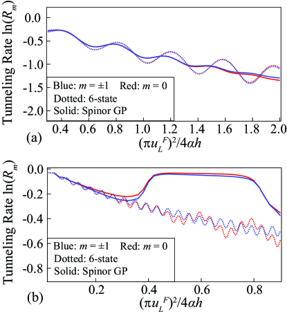
Figure 5: Spin-resolved tunneling rates $\ln(R_{m})$ obtained at $t_{\tau}=1$ versus the normalized inverse ramp rate $(\pi u_{L}^{F})^{2}/(4\alpha h)$ for (a) $\gamma=0.4$ and (b) $\gamma=1.5$. Solid red (blue) lines show 2D spinor GP simulation results for the $m=0$ ($m=\pm 1$) components. Dotted red (blue) lines show six-state model results for the $m=0$ ($m=\pm 1$) components. Except for $t_{\tau}$, the parameters are identical to those of Figs. 3(b) and 3(d).

To elucidate the challenges this poses (and to subsequently motivate why we use $t_{\tau}=0.2$ for the $\gamma=1.5$ measurements shown in Fig. 3(c)), Figs. 5(a) and 5(b) show the tunneling rates $R_{m}$ extracted at $t_{\tau}=1$ from spinor GP (solid lines) and six-state $c$-number (dotted lines) calculations for $\gamma=0.4$ and $\gamma=1.5$, respectively. For $\gamma=0.4$, no qualitative changes are observed compared to the results shown in Fig. 3(b), which uses $t_{\tau}=1.3$. Notably, though, the spinor GP results at $t_{\tau}=1$ show a smaller spin dependence than those at $t_{\tau}=1.3$, suggesting that internal dynamics of the BEC (i.e., evolution of the spatial density profile or in-trap motion) are enhanced for larger ramp times. For $\gamma=1.5$, in contrast, the behavior displayed in Fig. 5(b) (tunneling rate extracted at $t_{\tau}=1$) deviates significantly from that in Fig. 3(d) (tunneling rate extracted at $t_{\tau}=0.2$, which is approximately equal to the value of $t_{\tau}^{*}$ extracted in Fig. 2(b)). For $(\pi u_{L}^{F})^{2}/(4\alpha h)\lesssim 0.3$, which corresponds to ramps shorter than about $(t_{2}-t_{1})\approx 2.4$ ms, the tunneling rates for the six-state model oscillate around those for the spinor GP framework. These oscillations, and the lack thereof in the spinor GP calculations, are understood analogously to the $\gamma=0.4$ data presented in Figs. 5(a) and 3(b). However, the spinor GP framework yields tunneling rates that abruptly upshift towards zero at $(\pi u_{L}^{F})^{2}/(4\alpha h)\approx 0.3$. This upshift, which we attribute to non-negligible in-trap dynamics, is not captured by the more coarse-grained six-state model.

Specifically, the finite momentum component, which gets populated by the moving lattice, undergoes significant deceleration due to the ODT, making the distinction between the finite and the stationary $\mathbf{p}=0$ component more challenging for longer ramp times. When this happens, the interpretation of the dynamics within the six-state model is no longer possible. Moreover, in this regime ($(\pi u_{L}^{F})^{2}/(4\alpha h)\gtrsim 0.3$ for $\gamma=1.5$), the experiment no longer probes physics that can be meaningfully interpreted within the framework of tunneling physics. The data reported in Fig. 3(c) are thus taken at a $t_{\tau}$ value for which the momentum components can be resolved clearly, while maintaining $t_{\tau}\geq t_{\tau}^{*}$. We note that the value of $t_{\tau}^{*}$ is specific to our experimental parameters; it exploits, as explained in Appendix C, the relative narrowness of the transition.

Appendix E Validity of effective two-state description

The discussion of Fig. 2(c) shows that the six-state $c$-number Hamiltonian yields essentially spin-independent results for finite $c_{2}$ (using the value applicable for sodium). This behavior is accompanied, as shown in Fig. 3, by tunneling rates $\ln(R_{m})$ that are independent of $m$ for a good range of parameters. In both circumstances, the spin-independent predictions of the six-state model are essentially indistinguishable from those of the effective two-state $c$-number model (not shown).

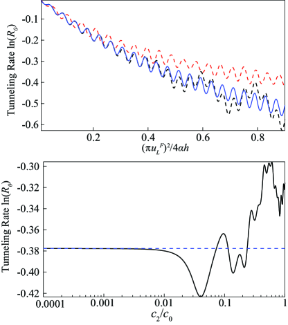
Figure 6: (a) Spin-resolved tunneling rates $\ln(R_{0})$ for the $m=0$ component obtained at $t_{\tau}=1$ and $\gamma=0.4$ versus the normalized inverse ramp rate $(\pi u_{L}^{F})^{2}/(4\alpha h)$. All data are predictions of the six-state model using $c_{2}/c_{0}=0$ (blue solid line), $c_{2}/c_{0}=0.036$ (black dashed line), and $c_{2}/c_{0}=1$ (red dashed line). (b) Tunneling rate $\ln(R_{0})$ obtained at fixed normalized inverse ramp rate $(\pi u_{L}^{F})^{2}/(4\alpha h)=0.5$ as a function of the relative strength $c_{2}/c_{0}$ of the spin-dependent and spin-independent interactions. The predictions of the six-state model are shown as the black solid line. For comparison, the horizontal blue dashed line shows the $c_{2}/c_{0}=0$ result, which is equivalent to the two-state model for the chosen initial state. Both panels use $q/h=42$ Hz.

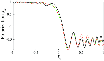
Figure 7: Polarization $J_{m}$, predicted by the six-state $c$-number model with finite $c_{2}$, as a function of the dimensionless time $t_{\tau}$ for an initial state with spinor phases $\theta_{0}=0$ and $\theta_{2}=-\pi$ at $t_{\tau}=-1$; this is to be contrasted with all other simulations shown in this paper, which initialize the system using $\theta_{0}=\theta_{2}=0$ at $t_{\tau}=-1$. The black solid, green dashed, and red dash-dotted lines show results for $m=0$, $m=-1$, and $m=+1$, respectively. The simulation parameters are $u_{L}^{F}=1.2$ $E_{R}$ (corresponding to $\gamma=0.4$), $q/h=42$ Hz, and $\alpha=4.5E_{R}$/ms. The full ramp from $t_{\tau}=-1$ to $t_{\tau}=1$ takes $1.8$ ms. The dimensionless inverse ramp rate $(\pi u_{L}^{F})^{2}/(4\alpha h)$ is equal to $2.6$.

Figure 6 investigates how the breakdown of the mapping between the six- and two-state models emerges as the relative contribution of the spin-dependent interactions, characterized by $c_{2}/c_{0}$, is varied. Figure 6(a) shows the six-state model tunneling rate $\ln(R_{0})$ with: (i) spin-dependent interactions turned off, i.e., $c_{2}/c_{0}=0$ (blue solid line); (ii) $c_{2}/c_{0}=0.036$ (black dashed line); and (iii) $c_{2}/c_{0}=1$ (red dashed line). In all three cases, the spin-independent nonlinearity $\gamma$ is set to $0.4$. Since the initial state does not contain a phase factor, the $c_{2}/c_{0}=0$ curve coincides with that for the two-state model (not shown). The value $c_{2}/c_{0}=0.036$ describes the sodium system. In the $(\pi u_{L}^{F})^{2}/(4\alpha h)\to 0$ limit, all three tunneling rate curves approach—as they should—zero. As the ramp rate is reduced (i.e., $(\pi u_{L}^{F})^{2}/(4\alpha h)$ is increased), the $c_{2}/c_{0}=0$ and $0.036$ curves are nearly indistinguishable for $(\pi u_{L}^{F})^{2}/(4\alpha h)\lesssim 0.3$. In this regime, the ramps are shorter than about $(t_{2}-t_{1})\approx 0.2$ ms on an absolute scale, so that $c_{2}(t_{2}-t_{1})/h$ is very small; correspondingly, the mixing of the different Zeeman states by spin-dependent interactions is expected to be very weak and insufficient to introduce an appreciable spin-dependence into the tunneling dynamics. As $(\pi u_{L}^{F})^{2}/(4\alpha h)$ increases further, the tunneling rates for $c_{2}/c_{0}=0$ and $0.036$ start to deviate. The tunneling rate for $c_{2}/c_{0}=1$ agrees quite well, except for a phase shift, with those for the smaller $c_{2}/c_{0}$ for $(\pi u_{L}^{F})^{2}/(4\alpha h)\lesssim 0.2$ but breaks away from those for the smaller $c_{2}/c_{0}$ for $(\pi u_{L}^{F})^{2}/(4\alpha h)\gtrsim 0.2$. Averaging over the oscillations can be seen to yield non-exponential behavior for $c_{2}/c_{0}\approx 1$ at $\gamma=0.4$.

Figure 6(b) shows the $m=0$ tunneling rate $\mathrm{ln}(R_{0})$, calculated at $t_{\tau}=1$, as a function of $c_{2}/c_{0}$ for $(\pi u_{L}^{F})^{2}/(4\alpha h)=0.5$. For $c_{2}/c_{0}\lesssim 0.02$, the six-state model tunneling rates (black solid line) remain very close to the $c_{2}/c_{0}=0$ result (blue dashed horizontal line), which coincides with the two-state model tunneling rates. Increasing the spin-dependent interactions beyond $c_{2}/c_{0}\approx 0.02$ leads to deviations between the two- and six-state model tunneling rates, consistent with the fact that the mapping from the six- to the two-state model is expected to lose its meaning as $c_{2}(t_{2}-t_{1})/h$ or $c_{2}/c_{0}$ become non-negligible.

Section III points out that the two-state description assumes a specific initial state. To demonstrate this explicitly, Fig. 7 shows six-state model results for $J_{m}$ as a function of the normalized ramp time $t_{\tau}$ for an initial state that differs from what we have been using up to now, namely for a state that is characterized by a non-vanishing spinor phase $\theta_{2}=-\pi$ and vanishing spinor phase $\theta_{0}=0$, where $\theta_{k}=\alpha_{-1,k}+\alpha_{1,k}-2\alpha_{0,k}$ and $d_{m,k}(t)$ is equal to $|d_{m,k}(t)|\exp(\imath\alpha_{m,k}(t))$. To allow for the phase imprinting, the initial state preparation follows a modified protocol: Starting with a state characterized by $d_{0,0}=1$ and all other $d_{m,k}=0$, the increase of the lattice depth is simulated. Population is redistributed and the finite phase $\theta_{2}$ is imprinted after the lattice depth has reached its final value such that $|d_{0,0}|^{2}+|d_{0,2}|^{2}=1/2$, $|d_{\pm 1,0}|^{2}+|d_{\pm 1,2}|^{2}=1/4$, $\theta_{0}=0$, and $\theta_{2}=-\pi$. Figure 7 shows that the non-zero value of $c_{2}$ leads to a spin dependence of the polarizations $J_{m}$; specifically, the solid black line for $m=0$ differs from the green dashed and red dash-dotted lines for $m=\pm 1$. This behavior cannot be captured by the effective two-state $c$-number model. We emphasize that the non-vanishing spinor phase $\theta_{2}$ is critical for observing the spin dependence.

The breakdown of the mapping between the six- and two-state models can also be driven by factors that are beyond the scope of a $c$-number model. For example, evolution of the (inhomogeneous) density profile of the condensate, in-trap dynamics, and the occupation of higher momentum states (i.e., outside the $\mathbf{p}=0$ and $2\hbar\mathbf{k}_{L}$ components we consider). This is consistent with observations throughout the main text and appendices wherein spin dependent tunneling dynamics is more readily observed in spinor GP predictions as opposed to those obtained from the $c$-number model.