Federated Learning: You May Communicate Less Often!

Abstract

We investigate the generalization error of statistical learning models in a Federated Learning (FL) setting. Specifically, we study the evolution of the generalization error with the number of communication rounds between the clients and the parameter server, i.e., the effect on the generalization error of how often the local models as computed by the clients are aggregated at the parameter server. We establish PAC-Bayes and rate-distortion theoretic bounds on the generalization error that account explicitly for the effect of the number of rounds, say $R\in\mathbb{N}$, in addition to the number of participating devices $K$ and individual datasets size $n$. The bounds, which apply in their generality for a large class of loss functions and learning algorithms, appear to be the first of their kind for the FL setting. Furthermore, we apply our bounds to FL-type Support Vector Machines (FSVM); and we derive (more) explicit bounds on the generalization error in this case. In particular, we show that the generalization error of FSVM increases with $R$, suggesting that more frequent communication with the parameter server diminishes the generalization power of such learning algorithms. Combined with that the empirical risk generally decreases for larger values of $R$, this indicates that $R$ might be a parameter to optimize in order to minimize the population risk of FL algorithms. Moreover, specialized to the case $R=1$ (sometimes referred to as “one-shot” FL or distributed learning) our bounds suggest that the generalization error of the FL setting decreases faster than that of centralized learning by a factor of $\mathcal{O}(\sqrt{\log(K)/K})$, thereby generalizing recent findings in this direction to arbitrary loss functions and algorithms. The results of this paper are also validated on some experiments.

1 Introduction

A major focus of machine learning research over recent years has been the development of statistical learning algorithms that can apply to data that is spatially distributed. In part, this is due to the emergence of new applications for which it is either not possible (due to lack of resources (Zinkevich et al., 2010; Kairouz et al., 2021)) or not desired (due to privacy concerns (Truex et al., 2019; Wei et al., 2020; Mothukuri et al., 2021)) to collect all the data at one point prior to applying a suitable machine learning algorithm to it (Verbraeken et al., 2020; McMahan et al., 2017; Konečnỳ et al., 2016; Kasiviswanathan et al., 2011). One popular such algorithm is the Federated-Learning (FL) of (McMahan et al., 2017) and many variants of it (Yang et al., 2018; Kairouz et al., 2019; Li et al., 2020; Reddi et al., 2020; Karimireddy et al., 2020; Yuan et al., 2021). In FL, there are $K$ clients or devices that hold each an own dataset $S_{k}$ and which collaborate to collectively train a (global) model by performing both local computations and updates based on multiple rounds interactions with a parameter server (PS). The model is depicted in Figure 1. Let $R\in\mathbb{N}^{*}$ denote the number of communication rounds. During each round $r=1,\ldots,R$, local computations at device $k\in\{1,\ldots,K\}$ are performed using some algorithm $\mathcal{A}_{k}$ in order to produce a local model $W^{(r)}_{k}$ — the notation will become clearer in the rest of this paper; at this level, we just hasten to mention that the subscript indicates the index of the client and the upper-script that of the round. Also, we emphasize that the individual datasets $\{S_{k}\}_{k}$ may be identically distributed across the devices (so-called homogeneous or i.i.d. setting) or not (heterogeneous or non i.i.d. setting); have the same size or not; and the algorithms $\{\mathcal{A}_{k}\}$ applied by the devices may be identical or not. A prominent example for the local algorithm $\mathcal{A}_{k}$ is the popular Stochastic Gradient Descent (SGD) where in each round every device takes one or more gradient steps with respect to samples from its local data $S_{k}$. At the end of every round $r$, all the devices send their individual models $\{W^{(r)}_{k}\}$ to the PS which aggregates them into a (global), possibly richer, model $\mkern 1.5mu\overline{\mkern-1.5muW\mkern-1.5mu}\mkern 1.5mu^{(r)}$ and sends it back to them. This aggregated model $\mkern 1.5mu\overline{\mkern-1.5muW\mkern-1.5mu}\mkern 1.5mu^{(r)}$ is then used by every device in the next round $(r+1)$, typically as an initialization point for the application of the algorithm $\mathcal{A}_{k}$ during that round but more general forms of statistical dependencies are allowed. The procedure is repeated until all the $R$ rounds are completed. The rationale is that the individually learned models are refined progressively by taking into account the data held by other devices; and, this way, at the end of the last round, all relevant features of all available datasets are captured by the final aggregated model $\mkern 1.5mu\overline{\mkern-1.5muW\mkern-1.5mu}\mkern 1.5mu^{(R)}$.

Figure 1: Multi-round Federated Learning model

The multi-round interactions with the PS are critical to the FL algorithm. Despite its importance, however, little is known about its effect on the performance of the algorithm. In fact, it was shown theoretically (Stich, 2019; Haddadpour et al., 2019; Qin et al., 2022), and also observed experimentally therein, that in FL-type algorithms the empirical risk generally decreases with the number of rounds. This observation is sometimes over-interpreted and it is believed that more frequent communication of the devices with the PS is generally beneficial for the performance of FL-type algorithms during inference or test phases. This belief was partially refuted in a very recent work (Chor et al., 2023) where it was shown that the generalization error may increase with the number of rounds. Their result, which is obtained by studying the evolution of a bound on the generalization error that they developed for their setup, relies strongly, however, on the assumed assumptions, named (i) linearity of the considered Bregman divergence loss with respect to the hypothesis, (ii) all the devices are constrained to run an SGD with mini-batch size one at every iteration and (iii) linearity of the aggregated model, set therein to be $\mkern 1.5mu\overline{\mkern-1.5muW\mkern-1.5mu}\mkern 1.5mu^{(r)}=\big{(}\sum_{k=1}^{K}W^{(r)}_{k}\big{)}/K$, with respect to the devices’ individual models. Also, in fact, even for the restricted setting considered therein, the bound on the generalization error that they developed (Chor et al., 2023, Theorem 1), which is essentially algebraic in nature, does not exploit fully the distributed architecture of the learning problem. Moreover, the dependence on the number of rounds is somewhat buried, at least in part, by decomposing the problem into several virtual one-client SGDs which are inter-dependent among clients and rounds through their initializations.

The effect of the multi-round interactions on the performance of FL algorithms remains highly unexplored, however, for general loss functions and algorithms. For example, with the very few exceptions that we discuss in this paper (most of which pertain to the specific case $R=1$ (Yagli et al., 2020; Barnes et al., 2022a, b; Sefidgaran et al., 2022a), and with relatively strong assumptions on the loss function and algorithm) the existing literature crucially lacks true bounds on the generalization error for FL-type algorithms, i.e., ones that bring the analysis of the distributed architecture and rounds into the bound, and even less that show some form of explicit dependency on $R$. One central mathematical difficulty in studying the behavior of the expected generalization error is caused by the interactions with the PS inducing statistical correlations among the devices models’ which become stronger with $R$ and are not easy to handle. For example, common tools that are generally applied in similar settings, such as the Leave-one-out Expansion Lemma of (Shalev-Shwartz et al., 2010), do not apply easily in this case.

In this paper, we study the problem of how the generalization error and population risk of FL-type algorithms evolve with the number of rounds $R$. Unless otherwise specified (for the specialization to Support Vector Machines in Section 4), we assume no particular form for the devices’ individual algorithms or aggregation function at the PS. That is, at every round $r$ each algorithm $\mathcal{A}_{k}$ is viewed as a general possibly stochastic conditional mapping $P_{W^{(r)}_{k}|S_{k}}$. Similarly, at every round $r$ the aggregation at the PS is viewed as a conditional mapping $P_{\mkern 1.5mu\overline{\mkern-1.5muW\mkern-1.5mu}\mkern 1.5mu^{(r)}|W^{(r)}_{1},\ldots,W^{(r)}_{K}}$. Also, we put no restriction on the loss function $\ell(\cdot,\cdot)$, except for a mild typical assumption on sub-Gaussianity and in Theorem 2 boundedness of the loss. For this (general) setting, first, we establish PAC-Bayes and rate-distortion theoretic bounds on the generalization error that account explicitly for the effect of the number of rounds $R$, in addition to the number of participating devices $K$ and the size of the dataset $n$. These bounds appear to be the first of their kind for the problem that we study. In particular, while most known PAC-Bayes bounds all pertain to centralized learning settings, our PAC-Bayes bounds (Theorems 1 and 2), which are tail bounds, can be viewed as judicious versions that are tailored specifically for the multi-client multi-round FL problem at hand. Also, interestingly, these bounds allow priors that are possibly distinct across devices and rounds. Our rate-distortion theoretic bounds (Theorem 3 and Theorem 4 of the appendix), which are in-expectation and tail bounds, have the desired property to show (i) how the generalization errors of the various devices at every round are coupled among them and (ii) how the contributions of the devices’ individual models to the generalization error of the final model $\mkern 1.5mu\overline{\mkern-1.5muW\mkern-1.5mu}\mkern 1.5mu^{(R)}$ evolve with the number of running rounds. For example, in Theorem 3 the contributions of the devices’ individual models to the overall generalization error are connected to individually allowed distortion levels $\epsilon_{r,k}$ that are linked to the total distortion level $\epsilon$ as $\epsilon=\big{(}\sum_{k=1}^{K}\sum_{r=1}^{R}\epsilon_{k,r}\big{)}/(KR)$. In a sense, this validates the intuition that, for a desired generalization error of the final model $\mkern 1.5mu\overline{\mkern-1.5muW\mkern-1.5mu}\mkern 1.5mu^{(R)}$, some devices may be allowed to overfit during some or all of the rounds as long as other devices compensate for that overfitting by, e.g., compressing further their inputs. That is, the targeted generalization error level of the final $\mkern 1.5mu\overline{\mkern-1.5muW\mkern-1.5mu}\mkern 1.5mu^{(R)}$ is suitably split among the devices and rounds.

Furthermore, we apply our bounds to Federated Support Vector Machines (FSVM); and we derive (more) explicit bounds on the generalization error in this case (Theorem 5). Importantly, we show that the margin generalization error of FSVM decreases with $K$ and increases with $R$. In particular, this suggests that more frequent communication with the PS diminishes the generalization power of FSVM algorithms. Combined with that that the empirical risk generally decreases for larger values of $R$, this indicates that $R$ might be a parameter to optimize in order to minimize the population risk of FL algorithms. Moreover, specialized to the case $R=1$ (sometimes referred to as “one-shot” FL or distributed learning) our bounds suggest that the generalization error of the FL setting decreases faster than that of centralized learning by a factor of $\mathcal{O}(\sqrt{\log(K)/K})$, thereby generalizing recent findings in this direction (Barnes et al., 2022a; Yagli et al., 2020; Sefidgaran et al., 2022a; Hu et al., 2023) to arbitrary loss functions and algorithms. We conduct experiments that validate our theoretical results.

We remark that in the particular case of FL-based SGD, at a high level there exists a connection between our setup, which is communication-oriented, and a growing body of literature on the assessment of the effect of batch and mini-batch sizes in centralized learning settings with SGD, i.e., so-called LocalSGD (Stich, 2019; Haddadpour et al., 2019; Qin et al., 2022; Gu et al., 2023). Specifically, our theoretical results suggest that even in that centralized setup one could still achieve some performance gains (from the viewpoint of generalization and population risk) by splitting the available entire dataset into smaller subsets, learning from each separately, aggregating the learned models, and then iterating. The aforementioned literature on this mostly reports improvements in convergence rates; and their proof techniques do not seem to be useful or applicable for the study of the generalization error. On the experimental side, it was already observed experimentally that the generalization error increases with the batch size (Jastrzebskii et al., 2017; Keskar et al., 2017).

Notations.

We denote random variables, their realizations, and their domains by upper-case, lower-case, and calligraphy fonts, e.g., $X$, $x$, and $\mathcal{X}$. We denote the distribution of $X$ by $P_{X}$ and its support by $\operatorname{supp}{P_{X}}$. A random variable $X$ is called $\sigma$-subgaussian, if for all $t\in\mathbb{R}$, $\log\mathbb{E}\left[\exp\left(t(X-\mathbb{E}[X])\right)\right]\leq\sigma^{2}t^{2}/2$, where $\mathbb{E}$ denote the expectation. For two distributions $P$ and $Q$ with the Radon-Nikodym derivative $\frac{\mathrm{d}Q}{\mathrm{d}P}$ of $Q$ with respect to $P$, the Kullback–Leibler (KL) divergence is defined as $D_{KL}\left(Q\|P\right)\coloneqq\mathbb{E}_{Q}\left[\log\frac{\mathrm{d}Q}{\mathrm{d}P}\right]$ if $Q\ll P$ and $\infty$ otherwise. The mutual information between two random variables $(X,Y)$ with distribution $P_{X,Y}$ and marginals $P_{X}$ and $P_{Y}$ is defined as $I(X;Y)\coloneqq D_{KL}\left(P_{X,Y}\|P_{X}P_{Y}\right)$. The notation $\{x_{i}\}_{i\in[m]}$ is used to denote a collection of $m$ real numbers. Similar notations are used to denote sets, distributions, or functions. The integer ranges $\{1,\ldots,K\}\subset\mathbb{N}$ and $\{K_{1},\ldots,K_{2}\}\subset\mathbb{N}$ are denoted by $[K]$ and $[K_{1}:K_{2}]$, respectively. Finally, for $k\in[K]$, we use the shorthand notation $[K]\setminus k\coloneqq\{1,\ldots,K\}\setminus\{k\}$.

2 Formal problem setup

Consider the $K$-client federated learning model shown in Figure 1. For $k\in[K]$, let $Z_{k}$ be some input data for client or device $k$ distributed according to an unknown distribution $\mu_{k}$ over some data space $\mathcal{Z}_{k}=\mathcal{Z}$. For example, in supervised learning settings $Z_{k}:=(X_{k},Y_{k})$ where $X_{k}$ stands for a data sample at device $k$ and $Y_{k}$ its associated label. The distributions $\{\mu_{k}\}$ are allowed to be distinct across the devices. The devices are equipped each with its own training dataset $S_{k}\coloneqq\{Z_{k,1},\dots,Z_{k,n}\}\subseteq\mathcal{Z}^{n}$, consisting of $n$ independent and identically distributed (i.i.d.) data points drawn according to the unknown distribution $\mu_{k}$. We consider an $R$-round learning framework, $R\in\mathbb{N}$, where every sample of a training dataset can be used during only one round by the device that holds it, but possibly multiple times during that round. Accordingly, it is assumed that every device partitions its data $S_{k}$ into $R$ disjoint subsets such that $S_{K}=\bigcup_{r\in[R]}S_{K}^{(r)}$ where $S_{k}^{(r)}$ is the dataset used by client $k\in[K]$ during round $r\in[R]$. This is a reasonable assumption that encompasses many practical situations in which at each round every client uses a new dataset. For ease of the exposition, we assume that $R$ divides $n$ and let $n_{R}\coloneqq n/R$ and $S_{k}^{(r)}\coloneqq\{Z_{k,1}^{(r)},\ldots,Z_{k,n_{R}}^{(r)}\}$. Also, throughout we will often find it convenient to use the handy notation $P_{S_{k}}\coloneqq\mu_{k}^{\otimes n}$, $P_{S_{k}^{(r)}}\coloneqq\mu_{k}^{\otimes n_{R}}$ and, for $k\in[K]$ and $r\in[R]$,

$$S_{[K]}^{(r)}= S_{1}^{(r)},\ldots,S_{K}^{(r)},\quad S_{[K]}^{[r]}= S_{1}^{[r]},\ldots,S_{k}^{[r]}=S_{[K]}^{(1)},\ldots,S_{[K]}^{(r)}$$

$$S_{k}^{[r]}= S_{k}^{(1)},\ldots,S_{k}^{(r)},\quad \mathbf{S}= S_{[K]}^{[R]}.$$ (1)

The devices collaboratively train a (global) model by performing both local computations and updates based on $R$-round interactions with the parameter server (PS). Let $\mathcal{A}_{k}$ denote the algorithm used by device $k\in[K]$. An example is the popular SGD where in round $r$ every device $k$ takes one or more gradient steps with respect to samples from the part $S^{(r)}_{k}$ of its local dataset $S_{k}$. It should be emphasized that the algorithms $\{\mathcal{A}_{k}\}$ may be identical or not. During round $r\in[R]$ the algorithm $\mathcal{A}_{k}$ produces a local model $W^{(r)}_{k}$. At the end of every round $r$, all the devices send their individual models $W^{(r)}_{k}$ to the PS which aggregates them into a (global) model $\mkern 1.5mu\overline{\mkern-1.5muW\mkern-1.5mu}\mkern 1.5mu^{(r)}\in\mathcal{W}$ and sends it back to them. The aggregated model is used by every device in the next round $(r+1)$, together with the part $S^{(r+1)}_{k}$ of its dataset $S_{k}$ in order to obtain a new local model $W^{(r+1)}_{k}$.

Formally, the algorithm $\mathcal{A}_{k}$ is a possibly stochastic mapping $\mathcal{A}_{k}\colon\mathcal{Z}^{n_{R}}\times\mathcal{W}\to\mathcal{W}$; and, for $r\in[R]$, we have $W_{k}^{(r)}\coloneqq\mathcal{A}_{k}(S_{k}^{(r)},\mkern 1.5mu\overline{\mkern-1.5muW\mkern-1.5mu}\mkern 1.5mu^{(r-1)})$ – for convenience, we set $\mkern 1.5mu\overline{\mkern-1.5muW\mkern-1.5mu}\mkern 1.5mu^{(0)}=\emptyset$ or some default value. Equivalently, we denote the distribution induced by $\mathcal{A}_{k}$ over $\mathcal{W}$ at round $r$ by the conditional $P_{W_{k}^{(r)}|S_{k}^{(r)},\mkern 1.5mu\overline{\mkern-1.5muW\mkern-1.5mu}\mkern 1.5mu^{(r-1)}}$. The aggregation function at the PS is set to be deterministic and arbitrary, such that at round $r$ this aggregation can be represented equivalently by a degenerate conditional distribution $P_{\mkern 1.5mu\overline{\mkern-1.5muW\mkern-1.5mu}\mkern 1.5mu^{r}|W_{[K]}^{(r)}}=P_{\mkern 1.5mu\overline{\mkern-1.5muW\mkern-1.5mu}\mkern 1.5mu^{r}|W_{1}^{(r)},\ldots,W_{K}^{(r)}}$. A common choice is the simple averaging $\mkern 1.5mu\overline{\mkern-1.5muW\mkern-1.5mu}\mkern 1.5mu^{(r)}=\big{(}\sum_{k=1}^{K}W^{(r)}_{k}\big{)}/K$.

The above process repeats until all $R$ rounds are completed, and yields a final (global) model $\mkern 1.5mu\overline{\mkern-1.5muW\mkern-1.5mu}\mkern 1.5mu^{(R)}$. Let $\mathbf{W}=\big{(}W_{[K]}^{[R]},\mkern 1.5mu\overline{\mkern-1.5muW\mkern-1.5mu}\mkern 1.5mu^{[R]}\big{)}$ where the notation used here and throughout is similar to (1). The above described algorithm induces the conditional distribution

$$P_{\mathbf{W}|\mathbf{S}}=\prod_{r\in[R]}\bigg{\{}\prod_{k\in[K]}\left(P_{W_{k}^{(r)}|S_{k}^{(r)},\mkern 1.5mu\overline{\mkern-1.5muW\mkern-1.5mu}\mkern 1.5mu^{(r-1)}}\right)\,P_{\mkern 1.5mu\overline{\mkern-1.5muW\mkern-1.5mu}\mkern 1.5mu^{(r)}|W_{[K]}^{(r)}}\bigg{\}},$$ (2)

whose joint distribution is

$$P_{\mathbf{S},\mathbf{W}}=\prod_{r\in[R]}\bigg{\{}\prod_{k\in[K]}\left(P_{S_{k}^{(r)}}P_{W_{k}^{(r)}|S_{k}^{(r)},\mkern 1.5mu\overline{\mkern-1.5muW\mkern-1.5mu}\mkern 1.5mu^{(r-1)}}\right)\,P_{\mkern 1.5mu\overline{\mkern-1.5muW\mkern-1.5mu}\mkern 1.5mu^{(r)}|W_{[K]}^{(r)}}\bigg{\}}.$$ (3)

Hereafter, we will refer to the aforementioned algorithm for short as being an $(P_{\mathbf{W}|\mathbf{S}},K,R,n)$-FL model.

Generalization error.

Let $\ell\colon\mathcal{Z}\times\mathcal{W}\to\mathbb{R}^{+}$ be a given loss function. For a (global) model or hypothesis $\mkern 1.5mu\overline{\mkern-1.5muw\mkern-1.5mu}\mkern 1.5mu^{(R)}\in\mathcal{W}$, its associated empirical and population risks are measured respectively as

$$\operatorname{\mathcal{\hat{L}}}\big{(}\mathbf{s},\mkern 1.5mu\overline{\mkern-1.5muw\mkern-1.5mu}\mkern 1.5mu^{(R)}\big{)} =\frac{1}{nK}\sum\nolimits_{k=1}^{K}\sum\nolimits_{i=1}^{n}\ell\big{(}z_{k,i},\mkern 1.5mu\overline{\mkern-1.5muw\mkern-1.5mu}\mkern 1.5mu^{(R)}\big{)},$$ (4a)

$$\mathcal{L}\big{(}\mkern 1.5mu\overline{\mkern-1.5muw\mkern-1.5mu}\mkern 1.5mu^{(R)}\big{)} =\frac{1}{K}\sum\nolimits_{k=1}^{K}\mathbb{E}_{Z_{k}\sim\mu_{k}}\big{[}\ell\big{(}Z_{k},\mkern 1.5mu\overline{\mkern-1.5muw\mkern-1.5mu}\mkern 1.5mu^{(R)}\big{)}\big{]}.$$ (4b)

Note that letting $\operatorname{\mathcal{\hat{L}}}\big{(}s_{k}^{(r)},\mkern 1.5mu\overline{\mkern-1.5muw\mkern-1.5mu}\mkern 1.5mu^{(R)}\big{)}=\frac{1}{n_{R}}\sum\nolimits_{i=1}^{n_{R}}\ell\big{(}z_{k,i}^{(r)},\mkern 1.5mu\overline{\mkern-1.5muw\mkern-1.5mu}\mkern 1.5mu^{(R)}\big{)}$, the empirical risk can be re-written as

$$\operatorname{\mathcal{\hat{L}}}\big{(}\mathbf{s},\mkern 1.5mu\overline{\mkern-1.5muw\mkern-1.5mu}\mkern 1.5mu^{(R)}\big{)}=\frac{1}{KR}\sum\nolimits_{r=1}^{R}\sum\nolimits_{k=1}^{K}\operatorname{\mathcal{\hat{L}}}\big{(}s_{k}^{(r)},\mkern 1.5mu\overline{\mkern-1.5muw\mkern-1.5mu}\mkern 1.5mu^{(R)}\big{)}.$$ (5)

The generalization error of the model $\mkern 1.5mu\overline{\mkern-1.5muw\mkern-1.5mu}\mkern 1.5mu^{(R)}$ for dataset $\mathbf{s}=(s_{1},\ldots,s_{K})$, $s_{k}=\bigcup_{r=1}^{R}s^{(r)}_{k}$, is evaluated as

$$\operatorname{gen}\big{(}\mathbf{s},\mkern 1.5mu\overline{\mkern-1.5muw\mkern-1.5mu}\mkern 1.5mu^{(R)}\big{)} =\mathcal{L}\big{(}\mkern 1.5mu\overline{\mkern-1.5muw\mkern-1.5mu}\mkern 1.5mu^{(R)}\big{)}-\operatorname{\mathcal{\hat{L}}}\big{(}\mathbf{s},\mkern 1.5mu\overline{\mkern-1.5muw\mkern-1.5mu}\mkern 1.5mu^{(R)}\big{)}=\frac{1}{KR}\sum\nolimits_{r=1}^{R}\sum\nolimits_{k=1}^{K}\operatorname{gen}\big{(}s_{k}^{(r)},\mkern 1.5mu\overline{\mkern-1.5muw\mkern-1.5mu}\mkern 1.5mu^{(R)}\big{)},$$ (6)

where $\operatorname{gen}\big{(}s_{k}^{(r)},\mkern 1.5mu\overline{\mkern-1.5muw\mkern-1.5mu}\mkern 1.5mu^{(R)}\big{)}=E_{Z_{k}\sim\mu_{k}}\big{[}\ell\big{(}Z_{k},\mkern 1.5mu\overline{\mkern-1.5muw\mkern-1.5mu}\mkern 1.5mu^{(R)}\big{)}\big{]}-\operatorname{\mathcal{\hat{L}}}\big{(}s_{k}^{(r)},\mkern 1.5mu\overline{\mkern-1.5muw\mkern-1.5mu}\mkern 1.5mu^{(R)}\big{)}$.

Example (FL-SGD).

An important example is one in which every device runs Stochastic Gradient Decent (SGD) or variants of it, such as mini-batch SGD. In this latter case, denoting by $e$ the number of epochs and by $b$ the size of the mini-batch, at iteration $t\in[e\,n_{R}/b]$ client $k$ updates its model as

$$W_{k,t}^{(r)}=\text{Proj}\left(W_{k,t-1}^{(r)}+\frac{\eta_{r,t}}{b}\sum\nolimits_{z\in\mathcal{B}_{k,r,t}}\nabla\tilde{\ell}\left(z,W_{k,t-1}^{(r)}\right)\right),$$ (7)

where $\tilde{\ell}\colon\mathcal{Z}\times\mathcal{W}\to\mathbb{R}^{+}$ is some differentiable surrogate loss function used for the optimization, $\eta_{r,t}\in\mathbb{R}^{+}$ is the learning rate at iteration $t$ of round $r$, $\mathcal{B}_{k,r,t}\in S_{k}^{(r)}$ is the mini-batch with size $b$ chosen at iteration $t$, and $\text{Proj}\big{(}w^{\prime}\big{)}=\operatorname*{arg\,min}_{w\in\mathcal{W}}\|w-w^{\prime}\|$. Also, in this case we let $W_{k}^{(r)}\coloneqq W_{k,\tau}^{(r)}$, where $\tau\coloneqq e\,n_{R}/b$. Besides, here the aggregation function at the PS is typically set to be the arithmetic average $\mkern 1.5mu\overline{\mkern-1.5muW\mkern-1.5mu}\mkern 1.5mu^{(r)}=\big{(}\sum_{k\in[K]}W_{k}^{(r)}\big{)}/K$. This example will be analyzed in the context of Support Vector Machines in Section 4.

3 Bounds on the generalization error of Federated Learning algorithms

In this section, we consider a (general) $(P_{\mathbf{W}|\mathbf{S}},K,R,n)$-FL algorithm, as defined formally in Section 2; and study the generalization error of the final (global) hypothesis $\mkern 1.5mu\overline{\mkern-1.5muW\mkern-1.5mu}\mkern 1.5mu^{(R)}$ as measured by (6). Note that the statistical properties of $\mkern 1.5mu\overline{\mkern-1.5muW\mkern-1.5mu}\mkern 1.5mu^{(R)}$ are described by the induced distributions (2) and (3). We establish several bounds on the generalization error (6). The bounds, which are of PAC-Bayes type and rate-distortion theoretic, have the advantage to take the structure of the studied multi-round interactive learning problem into account. Also, they account explicitly for the effect of the number of communication rounds $R$ with the PS, in addition to the number of devices $K$ and the size $n$ of each individual dataset. To the best of our knowledge, they are the first of their kind for this problem.

3.1 PAC-Bayes bounds

For convenience, we start with two lossless bounds, which can be seen as distributed versions of those of (McAllester, 1998, 1999; Maurer, 2004; Catoni, 2003) tailored specifically for the multiround interactive FL problem at hand.

Theorem 1

Assume that the loss $\ell(Z_{k},w)$ is $\sigma$-subgaussian for every $w\in\mathcal{W}$ and any $k\in[K]$. Let $\left\{\mathsf{P}_{k,r}\right\}_{k\in[K],r\in[R]}$ denote any set of priors such that $\mathsf{P}_{k,r}$ possibly depends on $\mkern 1.5mu\overline{\mkern-1.5muW\mkern-1.5mu}\mkern 1.5mu^{[r-1]}$, i.e., $\mathsf{P}_{k,r}$ is a conditional prior on $W^{(r)}_{k}$ given $\mkern 1.5mu\overline{\mkern-1.5muW\mkern-1.5mu}\mkern 1.5mu^{[r-1]}$. Then we have the following:

(i)

With probability at least $(1-\delta)$ over $\mathbf{S}$, for all $P_{\mathbf{W}|\mathbf{S}}$, $\mathbb{E}_{\mathbf{W}\sim P_{\mathbf{W}|\mathbf{S}}}\big{[}\operatorname{gen}(\mathbf{S},\mkern 1.5mu\overline{\mkern-1.5muW\mkern-1.5mu}\mkern 1.5mu^{(R)})\big{]}$ is bounded by

$$\sqrt{\frac{\frac{1}{KR}\sum_{k\in[K],r\in[R]}\mathbb{E}_{\mkern 1.5mu\overline{\mkern-1.5muW\mkern-1.5mu}\mkern 1.5mu^{[r-1]}\sim P_{\mkern 1.5mu\overline{\mkern-1.5muW\mkern-1.5mu}\mkern 1.5mu^{[r-1]}|S_{[K]}^{[r-1]}}}\left[D_{KL}\left(P_{W_{k}^{(r)}|S_{k}^{(r)},\mkern 1.5mu\overline{\mkern-1.5muW\mkern-1.5mu}\mkern 1.5mu^{(r-1)}}\|\mathsf{P}_{k,r}\right)\right]+\log(\frac{2n}{R\delta})}{(2n/R-1)/(4\sigma^{2})}}.$$

(ii)

For any FL-model $P_{\mathbf{W}|\mathbf{S}}$, with probability at least $(1-\delta)$ over $(\mathbf{S},\mathbf{W})\sim P_{\mathbf{S},\mathbf{W}}$,

$$\operatorname{gen}(\mathbf{S},\mkern 1.5mu\overline{\mkern-1.5muW\mkern-1.5mu}\mkern 1.5mu^{(R)})\leq\sqrt{\frac{\frac{1}{KR}\sum_{k\in[K],r\in[R]}\log\bigg{(}\frac{\mathrm{d}P_{W_{k}^{(r)}|S_{k}^{(r)},\mkern 1.5mu\overline{\mkern-1.5muW\mkern-1.5mu}\mkern 1.5mu^{(r-1)}}}{\mathrm{d}\mathsf{P}_{k,r}}\bigg{)}+\log(\frac{2n}{R\delta})}{(2n/R-1)/(4\sigma^{2})}}.$$

The proof of Theorem 1, which can be found in Appendix C.1, extends judiciously the technique of a variable-size compressibility approach that was proposed recently in (Sefidgaran and Zaidi, 2023) in the context of deriving data-dependent PAC-Bayes bounds for a centralized learning setting, i.e., $K=1$ and $R=1$, to the more involved setting of FL. Technically, one major difficulty in the analysis is accounting properly for the problem’s distributed nature as well as the statistical couplings among the devices’ models as induced by the multi-round interactions. It should be noted that, in fact, one could still consider the $R$-round FL problem end-to-end and view the entire system as a (virtual) centralized learning system with input the collection $\mathbf{S}=(S_{1},\ldots,S_{K})$ of all devices’ datasets and output the final aggregated model $\mkern 1.5mu\overline{\mkern-1.5muW\mkern-1.5mu}\mkern 1.5mu^{(R)}$ and apply the results of (Sefidgaran and Zaidi, 2023) (or those of (McAllester, 1998, 1999; Maurer, 2004; Catoni, 2003; Seeger, 2002; Tolstikhin and Seldin, 2013)). The results obtained that way, however, do not account for the interactive and distributed structure of the problem. In contrast, note that for example that the first bound of Theorem 1 involves, for each device $k$ and round $r$ the KL-divergence term $\mathbb{E}_{\mkern 1.5mu\overline{\mkern-1.5muW\mkern-1.5mu}\mkern 1.5mu^{[r-1]}}\left[D_{KL}\left(P_{W_{k}^{(r)}|S_{k}^{(r)},\mkern 1.5mu\overline{\mkern-1.5muW\mkern-1.5mu}\mkern 1.5mu^{(r-1)}}\|\mathsf{P}_{k,r}\right)\right]$ which can be seen as accounting for (a bound on) the contribution of the model of that client at that round $r$ to the overall generalization error. In a sense, the theorem says that only the average of those KL divergence terms matters for the bound, which could be interpreted as validating the intuition that some clients may be allowed to “overfit” during some or all of the rounds as long as the overall generalization error budget is controlled suitably by other devices. Also, as it can be seen from the result the choice of priors is specifically tailored for the multi-round multi-client setting in the sense that the prior of client $k$ at round $r$ could depend on all past aggregated models $\mkern 1.5mu\overline{\mkern-1.5muw\mkern-1.5mu}\mkern 1.5mu^{(r-1)}$ and $\mathsf{P}_{k}^{(r)}$ is allowed to depend on all local models and datasets till round $(r-1)$. The result also has implications on the design of practical learning FL systems: for example, on one aspect it suggests that the aforementioned KL-divergence term can be used as a round-dependent regularizer. In particular, this has the utility to allow to account better for the variation of the quality of the training datasets across devices and rounds.

Finally, we mention that viewing our studied learning setup with disjoint datasets along the clients and rounds as some form of distributed semi-online process, our Theorem 1 may be seen as a suitable distributed version of the PAC-Bayes bound of (Haddouche and Guedj, 2022) established therein for a centralized online-learning problem. Note that a direct extension of the result of (Haddouche and Guedj, 2022) to our distributed setup would imply considering the generalization error of client $k$ at round $r$ with respect to the intermediate aggregated model $\mkern 1.5mu\overline{\mkern-1.5muw\mkern-1.5mu}\mkern 1.5mu_{k}^{(r)}$, not the final $\mkern 1.5mu\overline{\mkern-1.5muw\mkern-1.5mu}\mkern 1.5mu_{k}^{(R)}$ as we do. In fact, in that case, the problem reduces to an easier virtual one-round setup that was also studied in (Barnes et al., 2022a, b) for Bregman divergences losses and linear and local Gaussian models; but at the expense of analyzing alternate quantity in place of the true generalization error (6) that we study.

We now present a more general, lossy, version of the bound of Theorem 1. The improvement is allowed by introducing a proper lossy compression that is defined formally below into the bound. This prevents the new bound from taking large values for deterministic algorithms with continuous hypothesis spaces.

Lossy compression.

Consider a quantization set $\mathcal{\hat{W}}\subseteq\mathcal{W}$ and let $\big{\{}\hat{W}_{k}^{(r)}\big{\}}_{k\in[K],r\in[R]}$, $\hat{W}_{k}^{(r)}\subseteq\mathcal{\hat{W}}$, be a set of lossy versions of $\big{\{}W_{k}^{(r)}\big{\}}_{k\in[K],r\in[R]}$, defined via some conditional Markov kernels $p_{\hat{W}_{k}^{(r)}|S_{k}^{(r)},\mkern 1.5mu\overline{\mkern-1.5muW\mkern-1.5mu}\mkern 1.5mu^{(r-1)}}$, i.e., we consider lossy compression of $W_{k}^{(r)}$ using only $S_{k}^{(r)}$ and the round-$(r-1)$ aggregated model $\mkern 1.5mu\overline{\mkern-1.5muW\mkern-1.5mu}\mkern 1.5mu^{(r-1)}$. For a given distortion level $\epsilon\in\mathbb{R}^{+}$, $\{p_{\hat{W}_{k}^{(r)}|S_{k}^{(r)},\mkern 1.5mu\overline{\mkern-1.5muW\mkern-1.5mu}\mkern 1.5mu^{(r-1)}}\}_{k\in[K],r\in[R]}$ is said to satisfy the $\epsilon$-distortion criterion if following holds: for every $\mathbf{s}\in\mathcal{Z}^{nK}$,

$$\bigg{|} \mathbb{E}_{P_{\mathbf{W}|\mathbf{s}}}\Big{[}\operatorname{gen}(\mathbf{s},\mkern 1.5mu\overline{\mkern-1.5muW\mkern-1.5mu}\mkern 1.5mu^{(R)})\Big{]}-\frac{1}{KR}\sum\nolimits_{k\in[K],r\in[R]}\mathbb{E}_{(Pp)_{k,r}}\Big{[}\operatorname{gen}(s_{k}^{(r)},\hat{\mkern 1.5mu\overline{\mkern-1.5muW\mkern-1.5mu}\mkern 1.5mu}^{(R)})\Big{]}\bigg{|}\leq\epsilon/2,$$ (8)

where

$$(Pp)_{k,r}=P_{\mkern 1.5mu\overline{\mkern-1.5muW\mkern-1.5mu}\mkern 1.5mu^{[r-1]},W_{[K]\setminus k}^{(r)}|s_{[K]}^{[r-1]},s_{[K]\setminus k}^{(r)}}\,p_{\hat{W}_{k}^{(r)}|s_{k}^{(r)},\mkern 1.5mu\overline{\mkern-1.5muW\mkern-1.5mu}\mkern 1.5mu^{(r-1)}}\,P_{\hat{\mkern 1.5mu\overline{\mkern-1.5muW\mkern-1.5mu}\mkern 1.5mu}^{(R)}|W_{[K]\setminus k}^{(r)},\hat{W}_{k}^{(r)},s_{[K]}^{[r+1:R]}}.$$

This condition can be simplified for Lipschitz losses, i.e., when $\forall w,w^{\prime}\in\mathcal{W}$, $|\ell(z,w)-\ell(z,w^{\prime})|\leq\mathfrak{L}\rho(w,w^{\prime})$, for some distortion function $\rho\colon\mathcal{W}\times\mathcal{W}\to\mathbb{R}^{+}$. Then, a sufficient condition for (8) is

$$\sum\nolimits_{k\in[K],r\in[R]}\mathbb{E}_{(Pp)_{k,r}P_{\mathbf{W}|\mathbf{s},\mkern 1.5mu\overline{\mkern-1.5muW\mkern-1.5mu}\mkern 1.5mu^{[r-1]},W_{[K]\setminus k}^{(r)}}}\Big{[}\rho(\mkern 1.5mu\overline{\mkern-1.5muW\mkern-1.5mu}\mkern 1.5mu^{(R)},\hat{\mkern 1.5mu\overline{\mkern-1.5muW\mkern-1.5mu}\mkern 1.5mu}^{(R)})\Big{]}\leq KR\epsilon/(4\mathfrak{L}).$$ (9)

Theorem 2

Suppose that $\ell(z,w)\in[0,C]\subset\mathbb{R}^{+}$. Consider any set of priors $\left\{\mathsf{P}_{k,r}\right\}_{k\in[K],r\in[R]}$ on $\{\hat{W}_{k}^{(r)}\}_{k\in[K],r\in[R]}$ such that $\mathsf{P}_{k,r}$ could depend on $\mkern 1.5mu\overline{\mkern-1.5muW\mkern-1.5mu}\mkern 1.5mu^{[r-1]}$, i.e., $\mathsf{P}_{k,r}$ is a conditional prior on $\hat{W}^{(r)}_{k}$ given $\mkern 1.5mu\overline{\mkern-1.5muW\mkern-1.5mu}\mkern 1.5mu^{[r-1]}$. Fix any distortion level $\epsilon\in\mathbb{R}^{+}$. Consider any $(P_{\mathbf{W}|\mathbf{S}},K,R,n)$-FL model and any choices of $\{p_{\hat{W}_{k}^{(r)}|S_{k}^{(r)},\mkern 1.5mu\overline{\mkern-1.5muW\mkern-1.5mu}\mkern 1.5mu^{(r-1)}}\}_{k\in[K],r\in[R]}$ that satisfy the $\epsilon$-distortion criterion. Then, with probability at least $(1-\delta)$ over $\mathbf{S}\sim P_{\mathbf{S}}$, we have that $\mathbb{E}_{\mathbf{W}\sim P_{\mathbf{W}|\mathbf{S}}}\left[\operatorname{gen}(\mathbf{S},\mkern 1.5mu\overline{\mkern-1.5muW\mkern-1.5mu}\mkern 1.5mu^{(R)})\right]$ is upper bounded by

$$\sqrt{\frac{\frac{1}{KR}\sum_{k\in[K],r\in[R]}\mathbb{E}_{\mkern 1.5mu\overline{\mkern-1.5muW\mkern-1.5mu}\mkern 1.5mu^{[r-1]}\sim P_{\mkern 1.5mu\overline{\mkern-1.5muW\mkern-1.5mu}\mkern 1.5mu^{[r-1]}|S_{[K]}^{[r-1]}}}\left[D_{KL}\left(p_{\hat{W}_{k}^{(r)}|S_{k}^{(r)},\mkern 1.5mu\overline{\mkern-1.5muW\mkern-1.5mu}\mkern 1.5mu^{(r-1)}}\|\mathsf{P}_{k,r}\right)\right]+\log(\frac{2n}{R\delta})}{(2n/R-1)/C^{2}}+\epsilon}.$$

This result, the proof of which is deferred to Appendix C.2, has novel aspects. First, instead of considering the quantization of the final aggregated model $W^{(R)}$, here for every $k\in[K]$ and round $r\in[R]$ we quantize the local model $W_{k}^{(r)}$ separately while keeping the other devices’ local models at that round, i.e., the vector $W_{[K]\setminus k}^{(r)}$, fixed. This allows us to study the amount of the “propagated” distortion till round $R$. Note that by quantizing $W_{k}^{(r)}$ for a distortion constraint on the generalization error that is at most $\nu$, the immediate aggregated model $\mkern 1.5mu\overline{\mkern-1.5muW\mkern-1.5mu}\mkern 1.5mu_{k}^{(r)}$ is guaranteed to have a generalization error which is within a distortion level of at most $\nu/K$ from the true value. Also, interestingly, the distortion criterion (8) allows to “allocate” suitably the targeted total distortion $KR\epsilon/2$ into smaller constituent levels among all clients and across all rounds.

3.2 Rate-distortion theoretic bounds

Define for $k\in[K]$, $r\in[R]$ and $\epsilon\in\mathbb{R}$, the rate-distortion function

$$\mathfrak{RD}(P_{\mathbf{S},\mathbf{W}},k,r,\epsilon)=\inf_{p_{\hat{W}_{k}^{(r)}|S_{k}^{(r)},\mkern 1.5mu\overline{\mkern-1.5muW\mkern-1.5mu}\mkern 1.5mu^{(r-1)}}}I(S_{k}^{(r)};\hat{W}_{k}^{(r)}|\mkern 1.5mu\overline{\mkern-1.5muW\mkern-1.5mu}\mkern 1.5mu^{(r-1)}),\vspace{-0.2cm}$$ (10)

where the mutual information is evaluated with respect to $P_{S_{k}^{(r)}}P_{\mkern 1.5mu\overline{\mkern-1.5muW\mkern-1.5mu}\mkern 1.5mu^{(r-1)}}p_{\hat{W}_{k}^{(r)}|S_{k}^{(r)},\mkern 1.5mu\overline{\mkern-1.5muW\mkern-1.5mu}\mkern 1.5mu^{(r-1)}}$ and the infimum is over all conditional Markov kernels $p_{\hat{W}_{k}^{(r)}|S_{k}^{(r)},\mkern 1.5mu\overline{\mkern-1.5muW\mkern-1.5mu}\mkern 1.5mu^{(r-1)}}$ that satisfy

$$\mathbb{E}_{\mathbf{S},\mathbf{W},\hat{\mkern 1.5mu\overline{\mkern-1.5muW\mkern-1.5mu}\mkern 1.5mu}^{(R)}}\left[\operatorname{gen}(S_{k}^{(r)},\mkern 1.5mu\overline{\mkern-1.5muW\mkern-1.5mu}\mkern 1.5mu^{(R)})-\operatorname{gen}(S_{k}^{(r)},\hat{\mkern 1.5mu\overline{\mkern-1.5muW\mkern-1.5mu}\mkern 1.5mu}^{(R)})\right]\leq\epsilon,\vspace{-0.2cm}$$ (11)

where the joint distribution of $\mathbf{S},\mathbf{W},\hat{\mkern 1.5mu\overline{\mkern-1.5muW\mkern-1.5mu}\mkern 1.5mu}^{(R)}$ factorizes as $P_{\mathbf{S},\mathbf{W}}p_{\hat{W}_{k}^{(r)}|S_{k}^{(r)},\mkern 1.5mu\overline{\mkern-1.5muW\mkern-1.5mu}\mkern 1.5mu^{(r-1)}}P_{\hat{\mkern 1.5mu\overline{\mkern-1.5muW\mkern-1.5mu}\mkern 1.5mu}^{(R)}|W_{[K]\setminus k}^{(r)},\hat{W}_{k}^{(r)}}$.

Theorem 3

For any $(P_{\mathbf{W}|\mathbf{S}},K,R,n)$-FL model with distributed dataset $\mathbf{S}\sim P_{\mathbf{S}}$, if the loss $\ell(Z_{k},w)$ is $\sigma$-subgaussian for every $w\in\mathcal{W}$ and any $k\in[K]$, then for every $\epsilon\in\mathbb{R}$ it holds that

$$\mathbb{E}_{\mathbf{S},\mathbf{W}\sim P_{\mathbf{S},\mathbf{W}}}\left[\operatorname{gen}(\mathbf{S},\mkern 1.5mu\overline{\mkern-1.5muW\mkern-1.5mu}\mkern 1.5mu^{(R)})\right]\leq\sqrt{\frac{2\sigma^{2}\sum_{k\in[K],r\in[R]}\mathfrak{RD}(P_{\mathbf{S},\mathbf{W}},k,r,\epsilon_{k,r})}{nK}}+\epsilon.$$

for any set of parameters $\{\epsilon_{k,r}\}_{k\in[K],r\in[R]}\subset\mathbb{R}$ which satisfy

$$\frac{1}{KR}\sum\nolimits_{k\in[K]}\sum\nolimits_{r\in[R]}\epsilon_{k,r}\leq\epsilon.$$

Similar to the PAC-Bayes type bounds of Theorem 1 and Theorem 2, the bound of Theorem 3 too shows the “contribution” of each client’s local model during each round to (a bound on) the generalization error as measured by (6). As it will become clearer from the below, an extended version of this theorem, which is stated in Appendix C.3, is particularly useful to study the Federated Support Vector Machines (FSVM) of the next section. For instance, an application of that result will yield a (more) explicit bound on the generalization error of FSVM in terms of the parameters $K$, $R$, and $n$.

We close this section by mentioning that we also report a tail rate-distortion theoretic bound. For this bound, let the randomness of the learning algorithm used by client $k\in[k]$ during round $r\in[R]$ be represented by some variable $U_{k}^{(r)}$, assumed to be independent of every other random variable. Denote $\mathbf{U}\coloneqq U_{[K]}^{[R]}$. This assumption implies that $W_{k}^{(r)}$ is a deterministic function of $S_{k}^{(r)}$, $U_{k}^{(r)}$, and the initialization $\mkern 1.5mu\overline{\mkern-1.5muW\mkern-1.5mu}\mkern 1.5mu^{(r-1)}$. For any fixed $\delta>0$, denote $\mathcal{G}_{P_{\mathbf{S},\mathbf{U},\mathbf{W}}}^{\delta}\coloneqq\left\{\nu_{\mathbf{S},\mathbf{U},\mathbf{W}}\colon D_{KL}\left(\nu_{\mathbf{S},\mathbf{U},\mathbf{W}}\|P_{\mathbf{S},\mathbf{U},\mathbf{W}}\right)\leq\log(1/\delta)\right\}$. Note that under $\nu$, for every $k\in[K]$ and $r\in[R]$, $W_{k}^{(r)}$ is a deterministic function of $S_{k}^{(r)}$, $U_{k}^{(r)}$ and $\mkern 1.5mu\overline{\mkern-1.5muW\mkern-1.5mu}\mkern 1.5mu^{(r-1)}$. Moreover, $\mkern 1.5mu\overline{\mkern-1.5muW\mkern-1.5mu}\mkern 1.5mu^{(r)}$ is a deterministic function of $W_{[K]}^{(r)}$. Hence, $\nu_{\mathbf{W}|\mathbf{S},\mathbf{U}}=P_{\mathbf{W}|\mathbf{S},\mathbf{U}}$. Also, let for given $\nu_{\mathbf{S},\mathbf{U},\mathbf{W}}$

$$\mathfrak{RD}(\nu_{\mathbf{S},\mathbf{U},\mathbf{W}},k,r,\epsilon)=\inf_{p_{\hat{W}_{k}^{(r)}|S_{k}^{(r)},U_{k}^{(r)},\mkern 1.5mu\overline{\mkern-1.5muW\mkern-1.5mu}\mkern 1.5mu^{(r-1)}}}I(S_{k}^{(r)};\hat{W}_{k}^{(r)}|U_{k}^{(r)},\mkern 1.5mu\overline{\mkern-1.5muW\mkern-1.5mu}\mkern 1.5mu^{(r-1)}),$$ (12)

where the mutual information is calculated with respect to $\nu_{S_{k}^{(r)},U_{k}^{(r)},\mkern 1.5mu\overline{\mkern-1.5muW\mkern-1.5mu}\mkern 1.5mu^{(r-1)}}p_{\hat{W}_{k}^{(r)}|S_{k}^{(r)},\mkern 1.5mu\overline{\mkern-1.5muW\mkern-1.5mu}\mkern 1.5mu^{(r-1)}}$ and the infimum is over all conditional Markov kernels $p_{\hat{W}_{k}^{(r)}|S_{k}^{(r)},\mkern 1.5mu\overline{\mkern-1.5muW\mkern-1.5mu}\mkern 1.5mu^{(r-1)}}$ that satisfy

$$\mathbb{E}_{\nu_{\mathbf{S},\mathbf{U},\mathbf{W}}}\Big{[}\operatorname{gen}(S_{k}^{(r)},\mkern 1.5mu\overline{\mkern-1.5muW\mkern-1.5mu}\mkern 1.5mu^{(R)})\Big{]}-\mathbb{E}_{\nu_{\mathbf{S},\mathbf{U}}(\nu p)_{k,r}}\Big{[}\operatorname{gen}(S_{k}^{(r)},\hat{\mkern 1.5mu\overline{\mkern-1.5muW\mkern-1.5mu}\mkern 1.5mu}^{(R)})\Big{]}\leq\epsilon,$$ (13)

with

$$(\nu p)_{k,r}= \nu_{\mkern 1.5mu\overline{\mkern-1.5muW\mkern-1.5mu}\mkern 1.5mu^{(r-1)},W_{[K]\setminus k}^{(r)}|S_{[K]}^{[r]}\setminus S_{k}^{(r)},U_{[K]}^{[r]}\setminus U_{k}^{(r)}}\,p_{\hat{W}_{k}^{(r)}|S_{k}^{(r)},U_{k}^{(r)},\mkern 1.5mu\overline{\mkern-1.5muW\mkern-1.5mu}\mkern 1.5mu^{(r-1)}}\,\nu_{\hat{\mkern 1.5mu\overline{\mkern-1.5muW\mkern-1.5mu}\mkern 1.5mu}^{(R)}|\hat{W}_{k}^{(r)},W_{[K]\setminus k}^{(r)},S_{[K]}^{[r+1:R]},U_{[K]}^{[r+1:R]}}.$$

It can be easily seen that this definition is consistent with (10).

Theorem 4

Consider a $(P_{\mathbf{W}|\mathbf{S}},K,R,n)$-FL model with distributed dataset $\mathbf{S}\sim P_{\mathbf{S}}$. Suppose that the loss $\ell(Z_{k},w)$ is $\sigma$-subgaussian for every $w\in\mathcal{W}$ and any $k\in[K]$. Fix any distortion level $\epsilon\in\mathbb{R}$. Then, for any $\delta>0$, with probability at least $(1-\delta)$, we have

$$\operatorname{gen}(\mathbf{S},\mkern 1.5mu\overline{\mkern-1.5muW\mkern-1.5mu}\mkern 1.5mu^{(R)})\leq\sqrt{\frac{\sup_{\nu_{\mathbf{S},\mathbf{U},\mathbf{W}}\in\mathcal{G}_{P_{\mathbf{S},\mathbf{U},\mathbf{W}}}^{\delta}}\sum_{k\in[K],r\in[R]}\mathfrak{RD}(\nu_{\mathbf{S},\mathbf{U},\mathbf{W}},k,r,\epsilon_{k,r})+\log(1/\delta)}{nK/(2\sigma^{2})}}+\epsilon,$$

for any $\{\epsilon_{k,r}\}_{k\in[K],r\in[R]}\subset\mathbb{R}$ such that

$$\frac{1}{KR}\sum\nolimits_{k\in[K]}\sum\nolimits_{r\in[R]}\epsilon_{k,r}\leq\epsilon.$$ (14)

In a sense, this result says that in order to have a good generalization performance (not only in-expectation as in Theorem 3 but also in terms of tails), the algorithm should be compressible not only under the true distribution $P_{\mathbf{S},\mathbf{W}}$ but also for all all those distributions $\nu_{\mathbf{S},\mathbf{U}}$ that are in the vicinity of $P_{\mathbf{S},\mathbf{U}}$.

4 Federated Support Vector Machines (FSVM)

In this section, we study the generalization behavior of the Support Vector Machines (SVM) (Cortes and Vapnik, 1995; Vapnik, 2006) when optimized in the FL setup using SGD. SVM is a popular algorithm that is used mainly in binary classification problems and is particularly powerful when used with high-dimensional kernels. For ease of exposition, however, we only consider linear SVMs; our results can be extended easily to any kernels.

Consider a binary classification problem in which $\mathcal{Z}=\mathcal{X}\times\mathcal{Y}$, $\mathcal{X}\subseteq\mathbb{R}^{d}$ with $\mathcal{Y}=\{-1,+1\}$. Using SVM for this problem consists in finding a suitable hyperplane, represented by $w\in\mathbb{R}^{d}$, that properly separates the data according to their labels. For convenience, we only consider the case with zero bias. In this case, the sign of the input $x\in\mathbb{R}^{d}$ is estimated using the sign of $\langle x,w\rangle$. The 0-1 loss $\ell_{0}\colon\mathcal{Z}\times\mathcal{W}\to\mathbb{R}^{+}$ is then evaluated as $\ell_{0}(z,w)\coloneqq\mathbbm{1}_{\{y\langle x,w\rangle>0\}}$. For the specific cases of centralized ($K=R=1$) and “one-shot” FL ($K\geq 2,R=1$) settings (Grønlund et al., 2020; Sefidgaran et al., 2022a), it was observed that if the algorithm finds a hyperplane that separates the data with some margin then it generalizes well. Motivated by this, we define the 0-1 margin loss function $\ell_{\theta}\colon\mathcal{Z}\times\mathcal{W}\to\mathbb{R}^{+}$ for $\theta\in\mathbb{R}^{+}$ as $\ell_{\theta}(z,w)\coloneqq\mathbbm{1}_{\{y\langle x,w\rangle>\theta\}}$. Similar to previous studies, we consider the empirical risk with respect to the margin loss, i.e., $\hat{\mathcal{L}}_{\theta}(\mathbf{s},\mkern 1.5mu\overline{\mkern-1.5muw\mkern-1.5mu}\mkern 1.5mu^{(R)})=\frac{1}{nK}\sum_{k\in[K],i\in[n]}\ell_{\theta}(z_{k,i},\mkern 1.5mu\overline{\mkern-1.5muw\mkern-1.5mu}\mkern 1.5mu^{(R)})$ which is equal to $\frac{1}{KR}\sum_{k\in[K],r\in[R]}\hat{\mathcal{L}}_{\theta}(\mathbf{s}_{k}^{r},\mkern 1.5mu\overline{\mkern-1.5muw\mkern-1.5mu}\mkern 1.5mu^{(R)})$. The population risk is considered with respect to 0-1 loss function $\ell_{0}$, i.e., $\mathcal{L}(\mkern 1.5mu\overline{\mkern-1.5muw\mkern-1.5mu}\mkern 1.5mu^{(R)})=\frac{1}{K}\sum_{k\in[K]}\mathbb{E}_{Z_{k}\sim\mu_{k}}\left[\ell_{0}(Z_{k},\mkern 1.5mu\overline{\mkern-1.5muw\mkern-1.5mu}\mkern 1.5mu^{(R)})\right]$. The margin generalization error is

$$\operatorname{gen}_{\theta}(\mathbf{s},\mkern 1.5mu\overline{\mkern-1.5muw\mkern-1.5mu}\mkern 1.5mu^{(R)})=\mathcal{L}(\mkern 1.5mu\overline{\mkern-1.5muw\mkern-1.5mu}\mkern 1.5mu^{(R)})-\hat{\mathcal{L}}_{\theta}(\mathbf{s},\mkern 1.5mu\overline{\mkern-1.5muw\mkern-1.5mu}\mkern 1.5mu^{(R)}).$$ (15)

The following mild assumptions on SGD are needed for the statement of the result that will follow.

Assumption 1

Consider an $(K,R,n,e,b)$-FL-SGD model. For every $r\in[2:R]$, every pair $(\mkern 1.5mu\overline{\mkern-1.5muw\mkern-1.5mu}\mkern 1.5mu^{(r-1)},\mkern 1.5mu\overline{\mkern-1.5muw\mkern-1.5mu}\mkern 1.5mu^{\prime(r-1)})$ and every $k\in[K]$, the following holds for any pair $(w_{k}^{(r)},w_{k}^{\prime(r)})$ that are both generated using $s_{k}^{(r)}$ with exactly similar mini-batches $\mathcal{B}_{k,r,t}\subseteq s_{k}^{(r)}$, $t\in[e\,n_{R}/b]$: there exists $q_{e,b}\in\mathbb{R}^{+}$ such that

$$\left\|w_{k}^{(r)}-w_{k}^{\prime(r)}\right\|\leq q_{e,b}\,\left\|\mkern 1.5mu\overline{\mkern-1.5muw\mkern-1.5mu}\mkern 1.5mu^{(r-1)}-\mkern 1.5mu\overline{\mkern-1.5muw\mkern-1.5mu}\mkern 1.5mu^{\prime(r-1)}\right\|.$$ (16)

If $q_{e,b}<1$, we say that SGD is contractive. The contractivity property of SGD was previously studied and theoretically proved under some assumptions, e.g., when the surrogate loss function $\tilde{\ell}$ is smooth and strongly convex as in (Dieuleveut et al., 2018; Park et al., 2022; Kozachkov et al., 2022). Note that in general the value of $q_{e,b}<1$ depends on the running round $r$ and learning rate $\eta_{r,t}$. In our case, as stated in Section 2, for simplicity we constrain the learning rates $\eta_{r,t}$ to be identical across devices and rounds; and, thus, the coefficients $q_{e,b}$ too are identical for all rounds. This is assumed only for the sake of simplicity; and the results that follow can be extended straightforwardly to the case of variable learning rates.

Now, denote the $d$-dimensional ball with origin center and radius $\nu>0$ as $\mathfrak{B}_{d}(\nu)$.

Assumption 2

Consider the $(K,R,n,e,b)$-FL-SGD model with $\mathcal{W}=\mathfrak{B}_{d}(1)$. Consider any $k\in[K]$, $r\in[2:R]$, and $\mkern 1.5mu\overline{\mkern-1.5muw\mkern-1.5mu}\mkern 1.5mu^{(r-1)}$. Fix some dataset $s_{k}^{(r)}$ as well as the mini-batches $\mathcal{B}_{k,r,t}\subseteq s_{k}^{(r)}$, $t\in[e\,n_{R}/b]$. Then, there exists a constant $\alpha\in\mathbb{R}^{+}$, such that for any $w_{\varepsilon}\in\mathcal{W}$,

$$\left\|w_{k}^{\prime(r)}-\left(w_{k}^{(r)}+\frac{1}{K}\mathsf{D}_{(\mkern 1.5mu\overline{\mkern-1.5muw\mkern-1.5mu}\mkern 1.5mu^{(r-1)},\{\mathcal{B}_{k,r,t}\}_{t})}\,w_{\varepsilon}\right)\right\|\leq\alpha\,\|w_{\varepsilon}\|^{2}/K^{2},$$ (17)

where $w_{k}^{(r)}$ and $w_{k}^{\prime(r)}$ are the local models of client $k$ at round $r$, when initialized by $\mkern 1.5mu\overline{\mkern-1.5muw\mkern-1.5mu}\mkern 1.5mu^{(r-1)}$ and $\mkern 1.5mu\overline{\mkern-1.5muw\mkern-1.5mu}\mkern 1.5mu^{(r-1)}+\frac{w_{\varepsilon}}{K}$, respectively, and when the same mini-batches $\{\mathcal{B}_{k,r,t}\}_{t}$ are used. Moreover, the matrix $\mathsf{D}_{(\mkern 1.5mu\overline{\mkern-1.5muw\mkern-1.5mu}\mkern 1.5mu^{(r-1)},\{\mathcal{B}_{k,r,t}\}_{t})}\in\mathbb{R}^{d\times d}$ represents the “overall gradient of SGD” of one client over one round, that depends on the initialization $\mkern 1.5mu\overline{\mkern-1.5muw\mkern-1.5mu}\mkern 1.5mu^{(r-1)}$ and mini-batches $\{\mathcal{B}_{k,r,t}\}_{t}$. We further assume that the spectral norm of this matrix is bounded by some $q_{e,b}$.

The inequality (17), which can be obtained using an easy expansion argument applied to the output of the perturbed initialization, is reasonable for moderate or large values of $K$, e.g., by assuming the boundedness of higher-order derivatives.

Now, we are ready to state our bound on the generalization error of FSVM.

Theorem 5

For FSVM optimized using $(K,R,n,e,b)$-FL-SGD with $\mathcal{W}=\mathfrak{B}_{d}(1)$, $\mathcal{X}=\mathfrak{B}_{d}(B)$ and $\theta\in\mathbb{R}^{+}$, if Assumptions 1 & 2 hold for some constants $q_{e,b}$ and $\alpha$ and if for $R\geq 2$, $K$ satisfies

$$K^{2}\geq\frac{\alpha}{{q_{e,b}}}\max\left(\frac{\alpha\,\max_{r^{\prime}\in[R-2]}(\sqrt{2}q_{e,b})^{2(R-r^{\prime})}}{q_{e,b}},\max_{r^{\prime}\in[R-1]}\frac{6Bq_{e,b}^{R-r^{\prime}}(1-(2q_{e,b})^{R-r^{\prime}})}{(1-2q_{e,b})\theta}\right),$$ (18)

then,

$$\mathbb{E}_{\mathbf{S},\mathbf{W}\sim P_{\mathbf{S},\mathbf{W}}}\left[\operatorname{gen}_{\theta}\left(\mathbf{S},\mkern 1.5mu\overline{\mkern-1.5muW\mkern-1.5mu}\mkern 1.5mu^{(R)}\right)\right] =\mathcal{O}\left(\sqrt{\frac{B^{2}\log(nK\sqrt{K})\sum_{r\in[R]}L_{r}}{nK^{2}\theta^{2}}}\right),$$ (19)

where

$$L_{r}=\inf_{t\geq q^{(R-r)}}\left\{t\log\max\left(\frac{K\theta}{Bt},\,2\right)\right\}\leq q_{e,b}^{2(R-r)}\log\max\left(\frac{K\theta}{Bq_{e,b}^{(R-r)}},\,2\right).$$ (20)

The theorem is proved in Appendix C.5 using an extended version of our rate-distortion theoretic lossy compression bound of Theorem 3, i.e., Proposition 6 (stated in Appendix A). To the best of our knowledge, this result is the first of its kind for this studied FSVM setting. We defer the discussion of some key elements of its proof technique to the below; and pause to state a few remarks that are in order. First, the bound of Theorem 5 shows an explicit dependence on the number of communication rounds $R$, in addition to the number of participating devices $K$ and the size of individual datasets $n$. In particular, the bound increases with $R$ for fixed $(n,K)$. This suggests that the generalization power of FSVM may diminish by more frequent communication with the PS (this theoretical finding will be illustrated below through some experiments). Combined with that the empirical risk generally decreases for larger values of $R$, this indicates that $R$ might be a hyper-parameter that needs to be optimized in order to minimize the population risk of FSVM. Equivalently, this means that during the training phase of such systems, one might choose deliberately to stop before convergence (at some appropriate round $R^{\star}\leq R$), accounting for the fact that while interactions that are beyond $R^{\star}$ indeed generally contribute to diminishing the empirical risk further their net effect on the true measure of performance, which is the population risk, may have a negative effect. Second, for fixed $(n,R)$ the bound improves (i.e., gets smaller) with $K$ with a factor of $\sqrt{\log(K)/K}$. This behavior was previously observed in different contexts and under different assumptions in (Sefidgaran et al., 2022a) and (Barnes et al., 2022a, b), but in both works only for the “one-shot” FL setting, i.e., $R=1$. In fact, it is easily seen that for the specific case $R=1$, the bound recovers the result of (Sefidgaran et al., 2022a, Theorem 5).

We now comment further on the result itself and its proof. First, it is insightful to note that, e.g., for $q_{e,b}<0.7$, the condition (18) on the number of participating devices $K$ for $q_{e,b}<0.7$ boils down to $K^{2}\geq\max(2\alpha^{2},6BR/\theta)$. Second, as can be found from its proof in the appendix section, for each $k\in[K]$ and $r\in[R]$ we first map the local models $W_{k}^{(r)}$ to a space with a smaller dimension of order $m_{r}=\mathcal{O}\left(\frac{B^{2}\log(nK\sqrt{K})\log(K/t)}{K^{2}\theta^{2}t^{2}}\right)$, for some $t\geq q^{(R-r)}$, using the Johnson-Lindenstrauss transformation (Johnson and Lindenstrauss, 1984). Then we quantize this mapped model. Applying quantization on a smaller dimension space is inspired by (Grønlund et al., 2020; Sefidgaran et al., 2022a); but with substantial extensions, however. In particular, we allow possibly different values of the dimensions for different values of $r$. For a contractive SGD, $m_{r}$ decreases with $r$. Then, we judiciously study the propagation of the quantization distortion until the end of round $R$. To do so, we first show that the intermediate aggregated model $\hat{W}_{k}^{(r)}=(\hat{W}_{k}^{(r)}+\sum_{j\neq k}W_{j}^{(r)})/K$ has a distortion level which is $K$ times smaller than that of $\hat{W}_{k}^{(r)}$. Then, we study the evolution of the distortion along the SGD iterations till the end of the round $R$. Intuitively, for the contractive SGD, the distortion decreases. This is why our $m_{r}$ decreases with $r$. For the non-contractive SGD, the opposite holds.

5 Experiments

We consider a binary classification problem, with two extracted classes (digits 1 and 6) of MNIST dataset (LeCun et al., 2010). Details of the experiments and further experiments are provided in Appendix B.

Figure 2: Generalization error (left plot) and bound of Theorem 5 (right plot) for $n=100$

Figure 3: Empirical risk (left plot) and population risk (right plot) for $n=100$

In Fig. 3, the (estimated) expected generalization error $\mathbb{E}_{\mathbf{S},\mathbf{W}}[\operatorname{gen}(\mathbf{S},\mkern 1.5mu\overline{\mkern-1.5muW\mkern-1.5mu}\mkern 1.5mu^{(R)}]$ and the computed bound of Theorem 5 are plotted versus the number of communication rounds $R$, for fixed $n=100$ and for $K\in\{10,20,50\}$. The expectation is estimated over $M=100$ Monte-Carlo simulations. As can be observed, for any value of $K$, the generalization error increases with $R$, as predicted by the bound of Theorem 5. Moreover, for any fixed $R$, both the generalization error and bound improve as $K$ increases.

Fig. 3 shows the empirical risk $\operatorname{\mathcal{\hat{L}}}(\mathbf{S},\mkern 1.5mu\overline{\mkern-1.5muW\mkern-1.5mu}\mkern 1.5mu^{(R)})$ and the (estimated) population risk $\mathcal{L}(\mkern 1.5mu\overline{\mkern-1.5muW\mkern-1.5mu}\mkern 1.5mu^{(R)})$, as functions of $R$. The population risk is estimated using the entire test dataset of MNIST, for the two classes, with $N_{test}=2093$. Interestingly, while the empirical risk keeps decreasing for $R\geq 5$, the population risk no longer decreases for beyond $R=5$. This numerically validates the claim that the population risk may “converge” faster than “empirical risk”. Hence, fewer rounds may be needed, if one can effectively take the “estimated” generalization error into account.

Appendices

The appendices are organized as follows:

• Appendix A contains further theoretical results. Specifically, this section contains extensions of all lossy bounds, i.e., extensions of Theorems 2, 3, and 4.

• Appendix B contains experiments details and further experiments, including:

  • experimental details in Appendix B,

  • experiment on FSVM for different values of $n$ in Appendix B.2,

  • experiment on FSVM in a heterogeneous data setting in Appendix B.3.

• Appendix C contains the deferred proofs of all our theoretical results.

  • Appendix C.1 contains the proof of Theorem 1,

  • Appendix C.2 contains the proof of Theorem 2,

  • Appendix C.3 contains the proof of Theorem 3,

  • Appendix C.4 contains the proof of Theorem 4,

  • Appendix C.5 contains the proof of Theorem 5,

  • Appendix C.6 contains the proof of Proposition 6,

  • Appendices C.7, C.8, C.9, and C.10 contain the proofs of Lemmas 9, 10, 11, and 12, respectively.

Appendix A Lossy compression bounds revisited

In all lossy bounds, i.e., Theorems 2, 3, and 4, we had three common assumptions on the quantizations of the local models:

• $\hat{\mathcal{W}}\subseteq\mathcal{W}$,

• the loss and generalization error definitions considered for the models $\hat{\mathcal{W}}$ are the same as the one considered for $\mathcal{W}$,

• the quantization of the model $W_{k}^{(r)}$ is performed according to $p_{\hat{W}_{k}^{(r)}|\mkern 1.5mu\overline{\mkern-1.5muW\mkern-1.5mu}\mkern 1.5mu^{(r-1)},S_{k}^{(r)}}$.

These choices are natural and intuitive ones for the FL learning algorithms. However, it turns out that all these conditions can be relaxed, i.e., in the following extended results, we consider

• $\hat{\mathcal{W}}$ to be any arbitrary set in $\mathbb{R}^{m}$, for some arbitrary $m\in\mathbb{N}$,

• the loss function $\hat{\ell}(z,\hat{w})\colon\mathcal{Z}\times\hat{\mathcal{W}}\to\mathbb{R}^{+}$ to be defined arbitrarily, possibly different than $\ell$. The generalization error for $\hat{\mathcal{W}}$ is defined then with respect to this loss function,

• for every $k\in[K]$ and $r\in[R]$, quantizing the aggregated global model $\hat{\mkern 1.5mu\overline{\mkern-1.5muW\mkern-1.5mu}\mkern 1.5mu}^{(R)}$ according to

  $$p_{\hat{\mkern 1.5mu\overline{\mkern-1.5muW\mkern-1.5mu}\mkern 1.5mu}_{k}^{(R)}|\mkern 1.5mu\overline{\mkern-1.5muW\mkern-1.5mu}\mkern 1.5mu^{(r-1)},S_{k}^{(r)},V_{k}^{(r)},W_{[K]\setminus k}^{(r)},S_{[K]}^{[r+1:R]},V_{[K]}^{[r+1:R]}},$$ (21)

  where $V_{k}^{(r)}\in\mathcal{V}$ presents some mutually independent available randomness used by client $k$ during round $r$. Note that unlike the Section 3.2, they do not necessarily represent all the randomness used by client $k$ during round $r$, e.g., they can be set to some constants or they can be set to be $U_{k}^{(r)}$ which is all the used randomness. Denote $\mathbf{V}=V_{[K]}^{[R]}$. Note that

  $$P_{\mathbf{S},\mathbf{V},\mathbf{W}}=P_{\mathbf{S}}P_{\mathbf{V}}P_{\mathbf{W}|\mathbf{S},\mathbf{V}}.$$ (22)

  The new choice of the quantization distribution implies that for every $k\in[K]$ and $r\in[R]$, in a sense we fix $\mkern 1.5mu\overline{\mkern-1.5muW\mkern-1.5mu}\mkern 1.5mu^{(r-1)},W_{[K]\setminus k}^{(r)},V_{[K]}^{[r+1:R]},S_{[K]}^{[r+1:R]}$, and consider quantization of the different global models obtained for different $S_{k}^{(r)}$.

Now, we state the extended results. For the following results, consider arbitrary set $\mathcal{{\hat{W}}}\in\mathbb{R}^{m}$, loss function $\hat{\ell}(z,\hat{w})$, and the generalization error that is defined with respect to this loss function. Next, we use the shorthand notation:

$$\mathfrak{V}_{k,r}=\left(V_{k}^{(r)},\mkern 1.5mu\overline{\mkern-1.5muW\mkern-1.5mu}\mkern 1.5mu^{(r-1)},W_{[K]\setminus k}^{(r)},S_{[K]}^{[r+1:R]},V_{[K]}^{[r+1:R]}\right).$$ (23)

First, we state the extended version of Theorem 3, that is used in the proof of Theorem 5. The proofs of these extended results follow the same lines as the original results. As an example, we show the proof of Proposition 6 in Appendix C.6. The rest of the proofs follow the proof of their corresponding theorems.

For $k\in[K]$, $r\in[R]$ and $\epsilon\in\mathbb{R}$, let $\mathcal{P}_{k,r}$ include all conditional Markov kernels

$$p_{\hat{\mkern 1.5mu\overline{\mkern-1.5muW\mkern-1.5mu}\mkern 1.5mu}_{k}^{(R)}|S_{k}^{(r)},\mathfrak{V}_{k,r}},$$ (24)

that satisfy

$$\mathbb{E}_{\mathbf{S},\mathbf{V},\mathbf{W},\hat{\mkern 1.5mu\overline{\mkern-1.5muW\mkern-1.5mu}\mkern 1.5mu}^{(R)}}\left[\operatorname{gen}(S_{k}^{(r)},\mkern 1.5mu\overline{\mkern-1.5muW\mkern-1.5mu}\mkern 1.5mu^{(R)})-\operatorname{gen}(S_{k}^{(r)},\hat{\mkern 1.5mu\overline{\mkern-1.5muW\mkern-1.5mu}\mkern 1.5mu}^{(R)})\right]\leq\epsilon,$$ (25)

where the joint distribution of $\mathbf{S},\mathbf{V},\mathbf{W},\hat{\mkern 1.5mu\overline{\mkern-1.5muW\mkern-1.5mu}\mkern 1.5mu}^{(R)}$ factorizes as $P_{\mathbf{S},\mathbf{V},\mathbf{W}}p_{\hat{\mkern 1.5mu\overline{\mkern-1.5muW\mkern-1.5mu}\mkern 1.5mu}_{k}^{(R)}|S_{k}^{(r)},\mathfrak{V}_{k,r}}$.

Now, define the rate-distortion function

$$\mathfrak{RD}^{\star}(P_{\mathbf{S},\mathbf{W}},k,r,\epsilon)=\inf_{\mathcal{P}_{k,r}}I(S_{k}^{(r)};\hat{\mkern 1.5mu\overline{\mkern-1.5muW\mkern-1.5mu}\mkern 1.5mu}_{k}^{(R)}|\mathfrak{V}_{k,r}),$$ (26)

where the mutual information is evaluated with respect to

$$P_{S_{k}^{(r)}}P_{\mathfrak{V}_{k,r}}\,p_{\hat{\mkern 1.5mu\overline{\mkern-1.5muW\mkern-1.5mu}\mkern 1.5mu}_{k}^{(R)}|S_{k}^{(r)},\mathfrak{V}_{k,r}}.$$ (27)

Proposition 6

For any $(P_{\mathbf{W}|\mathbf{S}},K,R,n)$-FL model with distributed dataset and randomness $(\mathbf{S},\mathbf{V})\sim P_{\mathbf{S}}P_{\mathbf{V}}$, if the loss $\ell(Z_{k},w)$ is $\sigma$-subgaussian for every $w\in\mathcal{W}$ and any $k\in[K]$, then for every $\epsilon\in\mathbb{R}$ it holds that

$$\mathbb{E}_{\mathbf{S},\mathbf{W}\sim P_{\mathbf{S},\mathbf{W}}}\left[\operatorname{gen}(\mathbf{S},\mkern 1.5mu\overline{\mkern-1.5muW\mkern-1.5mu}\mkern 1.5mu^{(R)})\right]\leq\sqrt{\frac{2\sigma^{2}\sum_{k\in[K],r\in[R]}\mathfrak{RD}^{\star}(P_{\mathbf{S},\mathbf{W}},k,r,\epsilon_{k,r})}{nK}}+\epsilon,$$

for any set of parameters $\{\epsilon_{k,r}\}_{k\in[K],r\in[R]}\subset\mathbb{R}$ which satisfy

$$\frac{1}{KR}\sum\nolimits_{k\in[K]}\sum\nolimits_{r\in[R]}\epsilon_{k,r}\leq\epsilon.$$

Next, we state the extension of Theorem 2.

Proposition 7

Suppose that $\ell(z,w)\in[0,C]\subset\mathbb{R}^{+}$. Consider any set of priors $\left\{\mathsf{P}_{k,r}\right\}_{k\in[K],r\in[R]}$ where $\mathsf{P}_{k,r}$ is a conditional prior on $\hat{\mkern 1.5mu\overline{\mkern-1.5muW\mkern-1.5mu}\mkern 1.5mu}^{(R)}$ given $\mathfrak{V}_{k,r}$. Fix any distortion level $\epsilon\in\mathbb{R}^{+}$. Consider any $(P_{\mathbf{W}|\mathbf{S}},K,R,n)$-FL model and any choices of

$$\left\{p_{\hat{\mkern 1.5mu\overline{\mkern-1.5muW\mkern-1.5mu}\mkern 1.5mu}_{k}^{(R)}|S_{k}^{(r)},\mathfrak{V}_{k,r}}\right\}_{k\in[K],r\in[R]},$$ (28)

that for every $\mathbf{s}\in\mathcal{Z}^{nK}$ satisfy the $\epsilon$-distortion criterion

$$\bigg{|} \mathbb{E}_{P_{\mathbf{W}|\mathbf{s}}}\Big{[}\operatorname{gen}(\mathbf{s},\mkern 1.5mu\overline{\mkern-1.5muW\mkern-1.5mu}\mkern 1.5mu^{(R)})\Big{]}-\frac{1}{KR}\sum\nolimits_{k\in[K],r\in[R]}\mathbb{E}_{(Pp)^{\star}_{k,r}}\Big{[}\operatorname{gen}(s_{k}^{(r)},\hat{\mkern 1.5mu\overline{\mkern-1.5muW\mkern-1.5mu}\mkern 1.5mu}^{(R)})\Big{]}\bigg{|}\leq\epsilon/2,$$ (29)

where

$$(Pp)_{k,r}^{\star}=P_{\mkern 1.5mu\overline{\mkern-1.5muW\mkern-1.5mu}\mkern 1.5mu^{[r-1]},W_{[K]\setminus k}^{(r)}|s_{[K]}^{[r-1]},s_{[K]\setminus k}^{(r)}}P_{V_{k}^{(r)},V_{[K]}^{[r+1:R]}}\,p_{\hat{\mkern 1.5mu\overline{\mkern-1.5muW\mkern-1.5mu}\mkern 1.5mu}^{(R)}|S_{k}^{(r)},\mathfrak{V}_{k,r}}.$$

Then, with probability at least $(1-\delta)$ over $\mathbf{S}\sim P_{\mathbf{S}}$, we have that $\mathbb{E}_{\mathbf{W}\sim P_{\mathbf{W}|\mathbf{S}}}\left[\operatorname{gen}(\mathbf{S},\mkern 1.5mu\overline{\mkern-1.5muW\mkern-1.5mu}\mkern 1.5mu^{(R)})\right]$ is upper bounded by

$$\sqrt{\frac{\frac{1}{KR}\sum_{k\in[K],r\in[R]}\mathbb{E}\left[D_{KL}\left(p_{\hat{\mkern 1.5mu\overline{\mkern-1.5muW\mkern-1.5mu}\mkern 1.5mu}_{k}^{(R)}|S_{k}^{(r)},\mathfrak{V}_{k,r}}\bigg{\|}\mathsf{P}_{k,r}\right)\right]+\log(\frac{2n}{R\delta})}{(2n/R-1)/C^{2}}+\epsilon},$$

where the expectations are with respect to $P_{\mkern 1.5mu\overline{\mkern-1.5muW\mkern-1.5mu}\mkern 1.5mu^{[r-1]},W_{[K]\setminus k}^{(r)}|s_{[K]}^{[r-1]},s_{[K]\setminus k}^{(r)}}P_{V_{k}^{(r)},V_{[K]}^{[r+1:R]}}$.

Finally, we present the extension of the rate-distortion theoretic tail bound. For the rest of this section, assume that $V_{k}^{(r)}=U_{k}^{(r)}$, for $k\in[K]$ and $r\in[R]$ and for a better clarity, denote $\mathfrak{V}_{k,r}$ by $\mathfrak{U}_{k,r}$ for this choice.

Consider any $\nu_{\mathbf{S},\mathbf{U},\mathbf{W}}\in\mathcal{G}_{P_{\mathbf{S},\mathbf{U},\mathbf{W}}}^{\delta}$. For this distribution and $k\in[K]$ and $r\in[R]$, let the $\mathcal{P}_{\nu,k,r}$ include all conditional Markov kernels

$$p_{\hat{\mkern 1.5mu\overline{\mkern-1.5muW\mkern-1.5mu}\mkern 1.5mu}_{k}^{(R)}|S_{k}^{(r)},\mathfrak{U}_{k,r}},$$ (30)

that satisfy

$$\mathbb{E}_{\mathbf{S},\mathbf{U},\mathbf{W},\hat{\mkern 1.5mu\overline{\mkern-1.5muW\mkern-1.5mu}\mkern 1.5mu}^{(R)}}\left[\operatorname{gen}(S_{k}^{(r)},\mkern 1.5mu\overline{\mkern-1.5muW\mkern-1.5mu}\mkern 1.5mu^{(R)})-\operatorname{gen}(S_{k}^{(r)},\hat{\mkern 1.5mu\overline{\mkern-1.5muW\mkern-1.5mu}\mkern 1.5mu}^{(R)})\right]\leq\epsilon,$$ (31)

where the expectation is with respect to $\nu_{\mathbf{S},\mathbf{U},\mathbf{W}}p_{\hat{\mkern 1.5mu\overline{\mkern-1.5muW\mkern-1.5mu}\mkern 1.5mu}_{k}^{(R)}|S_{k}^{(r)},\mathfrak{U}_{k,r}}$. Now, let

$$\mathfrak{RD}^{\star}(\nu_{\mathbf{S},\mathbf{U},\mathbf{W}},k,r,\epsilon)=\inf_{\mathcal{P}_{\nu,k,r}}I(S_{k}^{(r)};\hat{\mkern 1.5mu\overline{\mkern-1.5muW\mkern-1.5mu}\mkern 1.5mu}_{k}^{(R)}|\mathfrak{U}_{k,r}),$$ (32)

where the mutual information is calculated with respect to $\nu_{S_{k}^{(r)},\mathfrak{U}_{k,r}}p_{\hat{\mkern 1.5mu\overline{\mkern-1.5muW\mkern-1.5mu}\mkern 1.5mu}_{k}^{(R)}|S_{k}^{(r)},\mathfrak{U}_{k,r}}$.

Proposition 8

Consider a $(P_{\mathbf{W}|\mathbf{S}},K,R,n)$-FL model with distributed dataset and randomness $(\mathbf{S},\mathbf{U})\sim P_{\mathbf{S}}P_{\mathbf{U}}$. Suppose that the loss $\ell(Z_{k},w)$ is $\sigma$-subgaussian for every $w\in\mathcal{W}$ and any $k\in[K]$. Fix any distortion level $\epsilon\in\mathbb{R}$. Then, for any $\delta>0$, with probability at least $(1-\delta)$, we have

$$\operatorname{gen}(\mathbf{S},\mkern 1.5mu\overline{\mkern-1.5muW\mkern-1.5mu}\mkern 1.5mu^{(R)})\leq\sqrt{\frac{\sup_{\nu_{\mathbf{S},\mathbf{U},\mathbf{W}}\in\mathcal{G}_{P_{\mathbf{S},\mathbf{U},\mathbf{W}}}^{\delta}}\sum_{k\in[K],r\in[R]}\mathfrak{RD}^{\star}(\nu_{\mathbf{S},\mathbf{U},\mathbf{W}},k,r,\epsilon_{k,r})+\log(1/\delta)}{nK/(2\sigma^{2})}}+\epsilon,$$

for any $\{\epsilon_{k,r}\}_{k\in[K],r\in[R]}\subset\mathbb{R}$ such that

$$\frac{1}{KR}\sum\nolimits_{k\in[K]}\sum\nolimits_{r\in[R]}\epsilon_{k,r}\leq\epsilon.$$ (33)

Appendix B Additional experimental results & details

In this section, we first provide experimental and implementation details that were omitted in the main text. Then, some additional numerical simulations are shown and described.

B.1 Experimental & implementation details

Tasks description

In our experiments, we simulate a Federated Learning (FL) framework, according to the setup of this paper (see Section 1), on a single machine, where each “client” is an instance of the SVM model, equipped with a dataset. All tasks are performed on the same machine and we do not consider any communication constraint as it is not of interest in this paper. Once all clients’ models are trained, their weights are averaged and used by another instance of the SVM model (meant to be the one at the central server). This is utilized for computing the empirical risk $\hat{\mathcal{L}}_{\theta}(\mathbf{S},\mkern 1.5mu\overline{\mkern-1.5muW\mkern-1.5mu}\mkern 1.5mu)$ and population risk $\mathcal{L}(\mkern 1.5mu\overline{\mkern-1.5muW\mkern-1.5mu}\mkern 1.5mu)$. In particular, $\mathcal{L}(\mkern 1.5mu\overline{\mkern-1.5muW\mkern-1.5mu}\mkern 1.5mu)$ is estimated using a test set of fixed size $N_{test}=2093$. Using these quantities, the generalization error $\operatorname{gen}(\mathbf{S},\mkern 1.5mu\overline{\mkern-1.5muW\mkern-1.5mu}\mkern 1.5mu)$ is computed.

The (local) dataset of client # $k\in[K]$, denoted as $S_{k}$, is composed of $n$ samples that are drawn uniformly without replacement from $S$. In other words, the dataset $S$ is initially split into $K$ subsets. Each local dataset $S_{k}$ is then further split into $S_{k}^{(r)},\leavevmode\nobreak\ r\in[R]$ i.e., the training samples used at each round $r$ by client $k$.

Datasets

We consider a supervised learning setup, where the task is a binary image classification. More precisely, in our experiment, we train the SVM model to classify images of digits $1$ and $6$ from the standard MNIST (LeCun et al., 2010). Experiments were performed for different pairs of digits, giving similar results, and thus are not reported.

Model

Every client uses SVM with Radial Basis Function (RBF) kernel and applies Stochastic Gradient Descent (SGD) for optimization.

Training and hyperparameters

All models were trained with the same hyperparameters, which are given in Table 1. The data is scaled and normalized so as to get zero-mean and unit variance. All clients have the same adaptive learning rate $\eta_{t}$ i.e., at each round the learning rate is initialized with a value $\eta_{0}$ and, for each client, is multiplied by 0.2 whenever the training loss does not decrease by at least 0.01 for 10 consecutive local epochs. Note that a local epoch refers to a pass over the training samples at each round $r\in[R]$ i.e., $S_{k}^{(r)}$. Before each local epoch, $S_{k}^{(r)}$ is shuffled. The training algorithm ends when each client # $k\in[K]$ has done $e$ local epochs on each of the subsets $S_{k}^{(r)},\leavevmode\nobreak\ r\in[R]$.

Hyperparameter	Symbol	Value
Epochs	$e$	40
Initial learning rate	$\eta_{0}$	$0.01$
Batch size	$b$	$1$
Kernel parameter	$\gamma$	$0.05$
Dimension of the approximated kernel feature space	$d$	$4000$

Table 1: Hyperparameters

(a)

(b)

Figure 4: (a) Generalization error and (b) bound of Theorem 5 for $K=10$

(a)

(b)

Figure 5: (a) Empirical risk and (b) population risk for $K=10$

Hardware and implementation

We performed our experiments on a server equipped with 56 CPUs Intel Xeon E5-2690v4 2.60GHz.

The experiments are conducted using Python language. The open-source machine learning library scikit-learn (Pedregosa et al., 2011) is used to implement SVM. In particular, we use SGDClassifier to implement SGD optimization and RBFSampler for the Gaussian kernel feature map approximation.

B.2 Generalization error of FSVM for different values of $n$

Fig. 4 shows the (expected) generalization error (Subfig. 4(a)) of FSVM and the bound of Theorem 5 (Subfig. 4(b)) with respect to $R$ for $K=10$ fixed and $n\in\{100,200,500\}$. Fig. 5 shows the empirical risk and the estimated population risk.

These plots suggest that our observed behaviors in Section 5 hold for fixed $K$ and for various values of $n$. That is:

• The generalization error increases with $R$ for any fixed $n$,

• For any fixed $R$, both the generalization error and bound improve as $n$ increases,

• Above findings are compatible with the behavior predicted by the bound of Theorem 5,

• While the empirical risk keeps decreasing for $R\geq 5$, the population seems to have reached its minimum for $R=5$.

Note that similar results were obtained for other values of $n$.

B.3 Experiments for a heterogeneous data setting

We simulate a heterogeneous data setting (i.e., non-i.i.d.) by adding Gaussian white noise with standard deviation $\sigma=0.2$ to the training and testing images of a fraction $f=0.2$ of the clients. Therefore, as in the setup described in Section 1, the data distributions of clients $\mu_{k},\leavevmode\nobreak\ k\in[K]$ are different. The hyperparameters remain, however, identical as we aim at comparing the numerical results with the homogeneous data case.

Similar to Section 5, we compute the generalization error of FSVM, as well as the bound of Theorem 5, with respect to $R$ (see Fig. 6) and show the corresponding train and test risks (see Fig. 7).

The same observations can be made for the experiments in the homogeneous setting (Section 5). Remark that, on one hand, in comparison to Fig. 3, the empirical risk values on Fig. 7 are larger. This is expected, as the final global model is a simple arithmetic average of local models and hence may struggle to achieve the optimum of each local objective function in the presence of data heterogeneity. Therefore, more communication rounds $R$ are needed to achieve the same level of optimization as in the homogeneous case. On the other hand, the generalization error values (see Fig. 6) are smaller than in the i.i.d. setup (see Fig. 2). The global model is indeed less likely to overfit due to the “noise” that is injected into some of the local datasets.

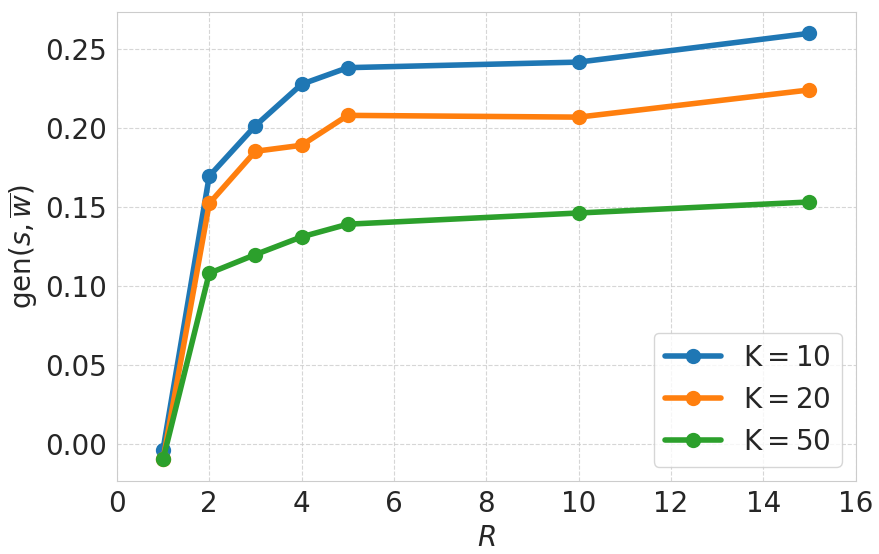
(a)

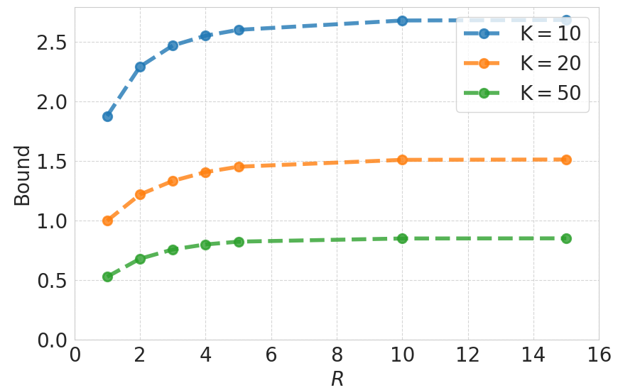
(b)

Figure 6: (a) Generalization error and (b) bound of Theorem 5 for $K=10$, non-iid setting

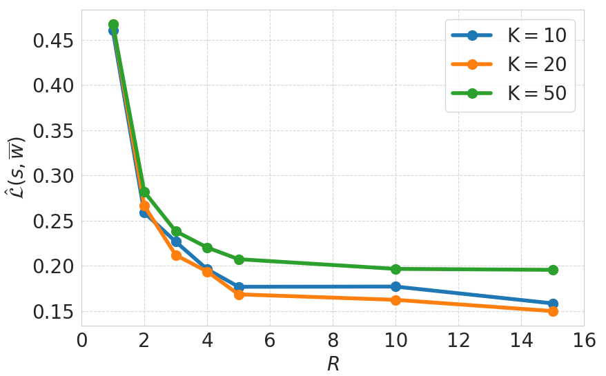
(a)

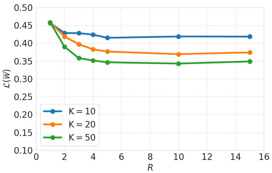
(b)

Figure 7: (a) Empirical risk and (b) population risk for $K=10$, non-iid setting

Appendix C Proofs

In this section, we provide the proofs of all theoretical results established in the paper and the appendices, by the order of their appearances.

C.1 Proof of Theorem 1

Without loss of generality assume $\sigma=1/2$, otherwise, consider the properly scaled loss function.

C.1.1 Part i.

Proof  The proof of this theorem is a particular case of Theorem 2, proved in Appendix C.2 for bounded losses and is similar for the $\sigma$-subgaussian case. We, however, provide the proof for the sake of completeness.

Similar to the proof of (Sefidgaran and Zaidi, 2023, Theorem 6), it is easy to see that for any choice of the prior $\mathsf{P}_{k,r}$, it suffices to only consider an arbitrary $P_{\mathbf{W}|\mathbf{S}}$. Now, let $\lambda\coloneqq 2n/R-1$. Let the RHS of the bound as $\sqrt{\Delta(\mathbf{S})}$, i.e., let

$$\Delta(\mathbf{S})\coloneqq \frac{\frac{1}{KR}\sum_{k\in[K],r\in[R]}\mathbb{E}_{\mkern 1.5mu\overline{\mkern-1.5muW\mkern-1.5mu}\mkern 1.5mu^{[r-1]}\sim P_{\mkern 1.5mu\overline{\mkern-1.5muW\mkern-1.5mu}\mkern 1.5mu^{[r-1]}|S_{[K]}^{[r-1]}}}\left[D_{KL}\left(p_{W_{k}^{(r)}|S_{k}^{(r)},\mkern 1.5mu\overline{\mkern-1.5muW\mkern-1.5mu}\mkern 1.5mu^{(r-1)}}\|\mathsf{P}_{k,r}\right)\right]+\log(\frac{2n}{R\delta})}{\lambda}.$$

Recall that

$$\mathbb{E}_{\mathbf{W}\sim P_{\mathbf{W}|\mathbf{S}}}\left[\operatorname{gen}(\mathbf{S},\mkern 1.5mu\overline{\mkern-1.5muW\mkern-1.5mu}\mkern 1.5mu^{(R)})\right]=\frac{1}{KR}\sum_{k\in[K],r\in[R]}\mathbb{E}_{\mathbf{W}\sim P_{\mathbf{W}|\mathbf{S}}}\left[\operatorname{gen}(S_{k}^{(r)},\mkern 1.5mu\overline{\mkern-1.5muW\mkern-1.5mu}\mkern 1.5mu^{(R)})\right].$$

Now, for any $\delta>0$,

$$\log \mathbb{P}_{\mathbf{S}}\left(\mathbb{E}_{\mathbf{W}\sim P_{\mathbf{W}|\mathbf{S}}}\left[\operatorname{gen}(\mathbf{S},\mkern 1.5mu\overline{\mkern-1.5muW\mkern-1.5mu}\mkern 1.5mu^{(R)})\right]>\sqrt{\Delta(\mathbf{S})}\right)$$

$$= \log\mathbb{P}_{\mathbf{S}}\left(\mathbb{E}_{\mathbf{W}\sim P_{\mathbf{W}|\mathbf{S}}}\left[\operatorname{gen}(\mathbf{S},\mkern 1.5mu\overline{\mkern-1.5muW\mkern-1.5mu}\mkern 1.5mu^{(R)})\right]^{2}>\Delta(\mathbf{S})\right)$$

$$\stackrel{{\scriptstyle(a)}}{{\leq}} \max\bigg{(}\log(\delta),\sup_{\nu_{\mathbf{S}}\in\mathcal{G}_{\mathbf{S}}^{\delta}}\bigg{\{}-D_{KL}(\nu_{\mathbf{S}}\|P_{\mathbf{S}})-\lambda\mathbb{E}_{\nu_{\mathbf{S}}}\left[\Delta(\mathbf{S})-\mathbb{E}_{\mathbf{W}\sim P_{\mathbf{W}|\mathbf{S}}}\left[\operatorname{gen}(\mathbf{S},\mkern 1.5mu\overline{\mkern-1.5muW\mkern-1.5mu}\mkern 1.5mu^{(R)})\right]^{2}\right]\bigg{\}}\bigg{)},$$

$$\stackrel{{\scriptstyle(b)}}{{\leq}} \max\bigg{(}\log(\delta),\sup_{\nu_{\mathbf{S}}\in\mathcal{G}_{\mathbf{S}}^{\delta}}\bigg{\{}-D_{KL}(\nu_{\mathbf{S}}\|P_{\mathbf{S}})-\lambda\mathbb{E}_{\nu_{\mathbf{S}}}\left[\Delta(\mathbf{S})-\frac{1}{KR}\sum_{k,r}\mathbb{E}_{\mathbf{W}\sim P_{\mathbf{W}|\mathbf{S}}}\left[\operatorname{gen}(S_{k}^{(r)},\mkern 1.5mu\overline{\mkern-1.5muW\mkern-1.5mu}\mkern 1.5mu^{(R)})^{2}\right]\right]\bigg{\}}\bigg{)},$$ (34)

where $(a)$ is shown in the next lemma, proved in Appendix C.7, and $(b)$ is due to the Jensen inequality.

Lemma 9

The inequality (34) holds.

Now, showing that the second term of (34) is bounded by $\log(\delta)$ completes the proof. For any $\mathbf{s}$ and any $k\in[K]$ and $r\in[R]$, we have

$$\lambda\mathbb{E}_{\nu_{\mathbf{S}}P_{\mathbf{W}|\mathbf{S}}}\left[\operatorname{gen}(S_{k}^{(r)},\mkern 1.5mu\overline{\mkern-1.5muW\mkern-1.5mu}\mkern 1.5mu^{(R)})^{2}\right]\stackrel{{\scriptstyle(a)}}{{\leq}} D_{KL}\Big{(}\nu_{\mathbf{S}}P_{\mathbf{W}|\mathbf{S}}\|P_{\mathbf{S}}(P\mathsf{P}_{k,r})_{k,r}\Big{)}+\log\mathbb{E}_{P_{\mathbf{S}}(P\mathsf{P}_{k,r})_{k,r}}\left[e^{\lambda\operatorname{gen}(s_{k}^{(r)},\hat{\mkern 1.5mu\overline{\mkern-1.5muW\mkern-1.5mu}\mkern 1.5mu}^{(R)})^{2}}\right]$$

$$\stackrel{{\scriptstyle(b)}}{{\leq}} D_{KL}\Big{(}\nu_{\mathbf{S}}P_{\mathbf{W}|\mathbf{S}}\|P_{\mathbf{S}}(P\mathsf{P}_{k,r})_{k,r}\Big{)}+\log(2n/R)$$

$$= \mathbb{E}_{\nu_{\mathbf{S}}P_{\mkern 1.5mu\overline{\mkern-1.5muW\mkern-1.5mu}\mkern 1.5mu^{[r-1]}|S_{[K]}^{[r-1]}}}\left[D_{KL}\Big{(}P_{W_{k}^{(r)}|S_{k}^{(r)},W^{(r-1)}}\|\mathsf{P}_{W_{k}^{(r)}|\mkern 1.5mu\overline{\mkern-1.5muW\mkern-1.5mu}\mkern 1.5mu^{[r-1]}}\Big{)}\right]$$

$$+ D_{KL}\Big{(}\nu_{\mathbf{S}}\|P_{\mathbf{S}}\Big{)}+\log(2n/R),$$

where $(a)$ holds by Donsker-Varadhan’s inequality, and where

$$(P\mathsf{P}_{k,r})_{k,r}\coloneqq P_{\mkern 1.5mu\overline{\mkern-1.5muW\mkern-1.5mu}\mkern 1.5mu^{[r-1]},W_{[K]\setminus k}^{(r)}|S_{[K]}^{[r-1]},S_{[K]\setminus k}^{(r)}}\mathsf{P}_{W_{k}^{(r)}|\mkern 1.5mu\overline{\mkern-1.5muW\mkern-1.5mu}\mkern 1.5mu^{[r-1]}}P_{\mkern 1.5mu\overline{\mkern-1.5muW\mkern-1.5mu}\mkern 1.5mu^{(R)}|W_{[K]}^{(r)},S_{[K]}^{[r+1:R]}},$$

and $(b)$ due to the fact that $\operatorname{gen}(s_{k}^{(r)},\hat{\mkern 1.5mu\overline{\mkern-1.5muW\mkern-1.5mu}\mkern 1.5mu}^{(R)})$ is $1/\sqrt{4n/R}$-subgaussian.

Combining the above inequality with (34) completes the proof.  

C.1.2 Part ii.

Proof  Consider any FL-model $P_{\mathbf{W}|\mathbf{S}}$. Consider any set of priors $\left\{\mathsf{P}_{k,r}\right\}_{k\in[K],r\in[R]}$ such that $\mathsf{P}_{k,r}$ could depend on $\mkern 1.5mu\overline{\mkern-1.5muW\mkern-1.5mu}\mkern 1.5mu^{[r-1]}$, i.e., $\mathsf{P}_{k,r}$ is a conditional prior on $W^{(r)}_{K}$ given $\mkern 1.5mu\overline{\mkern-1.5muW\mkern-1.5mu}\mkern 1.5mu^{[r-1]}$. Let $\lambda\coloneqq 2n/R-1$. Let the RHS of the bound as $\sqrt{\Delta(\mathbf{S},\mathbf{W})}$, i.e., let

$$\Delta(\mathbf{S},\mathbf{W})\coloneqq \frac{\frac{1}{KR}\sum_{k\in[K],r\in[R]}\log\left(\frac{\mathrm{d}P_{W_{k}^{(r)}|S_{k}^{(r)},\mkern 1.5mu\overline{\mkern-1.5muW\mkern-1.5mu}\mkern 1.5mu^{(r-1)}}}{\mathrm{d}\mathsf{P}_{k,r}r}\right)+\log(\frac{2n}{R\delta})}{\lambda}.$$

Further, recall that

$$\operatorname{gen}(\mathbf{S},\mkern 1.5mu\overline{\mkern-1.5muW\mkern-1.5mu}\mkern 1.5mu^{(R)})=\frac{1}{KR}\sum_{k\in[K],r\in[R]}\operatorname{gen}(S_{k}^{(r)},\mkern 1.5mu\overline{\mkern-1.5muW\mkern-1.5mu}\mkern 1.5mu^{(R)}).$$

Denote

$$(P\mathsf{P})_{k,r}\coloneq P_{\mkern 1.5mu\overline{\mkern-1.5muW\mkern-1.5mu}\mkern 1.5mu^{(r-1)},W_{[K]\setminus k}^{(r)}|S_{[K]}^{[r-1]},S_{[K]\setminus k}^{(r)}}\mathsf{P}_{k,r}P_{\mkern 1.5mu\overline{\mkern-1.5muW\mkern-1.5mu}\mkern 1.5mu^{(R)}|\mkern 1.5mu\overline{\mkern-1.5muW\mkern-1.5mu}\mkern 1.5mu^{(r)},S_{[K]}^{[r+1:R]}},\quad k\in[K],r\in[R].$$

Then,

$$\mathbb{P} \Big{(}\operatorname{gen}(\mathbf{S},\mkern 1.5mu\overline{\mkern-1.5muW\mkern-1.5mu}\mkern 1.5mu^{(R)})\geq\sqrt{\Delta(\mathbf{S},\mathbf{W})}\Big{)}$$ (35)

$$\stackrel{{\scriptstyle(a)}}{{\leq}} \mathbb{P}\Big{(}\frac{1}{KR}\sum_{k\in[K],r\in[R]}\operatorname{gen}(S_{k}^{(r)},\mkern 1.5mu\overline{\mkern-1.5muW\mkern-1.5mu}\mkern 1.5mu^{(R)})^{2}\geq\Delta(\mathbf{S},\mathbf{W})\Big{)}$$

$$\stackrel{{\scriptstyle(b)}}{{\leq}} \max\bigg{(}\log(\delta),\sup_{\nu_{\mathbf{c},\mathbf{W}}\in\mathcal{G}_{\mathbf{S},\mathbf{W}}^{\delta}}\bigg{\{}-D_{KL}(\nu_{\mathbf{S},\mathbf{W}}\|P_{\mathbf{S},\mathbf{W}})-\lambda\mathbb{E}_{\nu_{\mathbf{S},\mathbf{W}}}\left[\Delta(\mathbf{S},\mathbf{W})-\frac{1}{KR}\sum_{r,k}\operatorname{gen}(S_{k}^{(r)},\mkern 1.5mu\overline{\mkern-1.5muW\mkern-1.5mu}\mkern 1.5mu^{(R)})^{2}\right]\bigg{\}}\bigg{)},$$ (36)

where $(a)$ holds by Jensen inequality for the convex function $g(x)=x^{2}$ and $(b)$ is due Lemma 10, proved in Appendix C.8.

Lemma 10

The inequality (36) holds.

Next, note that using Donsker-Varadhan’s inequality we have

$$\mathbb{E}_{\nu_{\mathbf{S},\mathbf{W}}} \left[\lambda\operatorname{gen}(S_{k}^{(r)},\mkern 1.5mu\overline{\mkern-1.5muW\mkern-1.5mu}\mkern 1.5mu^{(R)})^{2}\right]$$

$$\leq \mathbb{E}_{\nu_{\mathbf{S}}}\left[D_{KL}\left(\nu_{\mathbf{W}|\mathbf{S}}\|(P\mathsf{P})_{k,r}\right)+\log\mathbb{E}_{(P\mathsf{P})_{k,r}}\left[e^{\lambda\operatorname{gen}(S_{k}^{(r)},\mkern 1.5mu\overline{\mkern-1.5muW\mkern-1.5mu}\mkern 1.5mu^{(R)})^{2}}\right]\right]$$

$$\leq D_{KL}\left(\nu_{\mathbf{S},\mathbf{W}}\|\nu_{\mathbf{S}}(P\mathsf{P})_{k,r}\right)+D_{KL}\left(\nu_{\mathbf{S}}\|P_{\mathbf{S}}\right)+\log\mathbb{E}_{P_{\mathbf{S}}(P\mathsf{P})_{k,r}}\left[e^{\lambda\operatorname{gen}(S_{k}^{(r)},\mkern 1.5mu\overline{\mkern-1.5muW\mkern-1.5mu}\mkern 1.5mu^{(R)})^{2}}\right]$$

$$\leq D_{KL}\left(\nu_{\mathbf{S},\mathbf{W}}\|\nu_{\mathbf{S}}(P\mathsf{P})_{k,r}\right)+D_{KL}\left(\nu_{\mathbf{S}}\|P_{\mathbf{S}}\right)+\log\left(2n/R\right)$$

$$= D_{KL}\left(\nu_{\mathbf{S},\mathbf{W}}\|\nu_{\mathbf{S}}P_{\mathbf{W}|\mathbf{S}}\right)+\mathbb{E}_{\nu_{\mathbf{S},\mathbf{W}}}\left[\log\left(\frac{\mathrm{d}P_{W_{k}^{(r)}|S_{k}^{(r)},\mkern 1.5mu\overline{\mkern-1.5muW\mkern-1.5mu}\mkern 1.5mu^{(r-1)}}}{\mathrm{d}\mathsf{P}_{k,r}r}\right)\right]+D_{KL}\left(\nu_{\mathbf{S}}\|P_{\mathbf{S}}\right)+\log\left(2n/R\right)$$

$$= D_{KL}\left(\nu_{\mathbf{S},\mathbf{W}}\|P_{\mathbf{S},\mathbf{W}}\right)+\mathbb{E}_{\nu_{\mathbf{S},\mathbf{W}}}\left[\log\left(\frac{\mathrm{d}P_{W_{k}^{(r)}|S_{k}^{(r)},\mkern 1.5mu\overline{\mkern-1.5muW\mkern-1.5mu}\mkern 1.5mu^{(r-1)}}}{\mathrm{d}\mathsf{P}_{k,r}r}\right)\right]+\log\left(2n/R\right).$$

Putting everything together conclude that

$$-D_{KL}(\nu_{\mathbf{S},\mathbf{W}}\|P_{\mathbf{S},\mathbf{W}})- \lambda\mathbb{E}_{\nu_{\mathbf{S},\mathbf{W}}}\left[\Delta(\mathbf{S},\mathbf{W})-\frac{1}{KR}\sum_{r,k}\operatorname{gen}(S_{k}^{(r)},\mkern 1.5mu\overline{\mkern-1.5muW\mkern-1.5mu}\mkern 1.5mu^{(R)})^{2}\right]\leq\log(\delta).$$

This completes the proof.

 

C.2 Proof of Theorem 2

Proof  Similar to the proof of (Sefidgaran and Zaidi, 2023, Theorem 6), it is easy to see that for any choice of the prior $\mathsf{P}_{k,r}$, it suffices to only consider an arbitrary $P_{\mathbf{W}|\mathbf{S}}$. Furthermore, without loss of generality, we can assume $C=1$, otherwise, one can re-scale the loss function.

Let $\lambda\coloneqq 2n/R-1$ and the RHS of the bound as $\sqrt{\Delta(\mathbf{S})}$, i.e., let

$$\Delta(\mathbf{S})\coloneqq \frac{\frac{1}{KR}\sum_{k\in[K],r\in[R]}\mathbb{E}_{\mkern 1.5mu\overline{\mkern-1.5muW\mkern-1.5mu}\mkern 1.5mu^{[r-1]}\sim P_{\mkern 1.5mu\overline{\mkern-1.5muW\mkern-1.5mu}\mkern 1.5mu^{[r-1]}|S_{[K]}^{[r-1]}}}\left[D_{KL}\left(p_{\hat{W}_{k}^{(r)}|S_{k}^{(r)},\mkern 1.5mu\overline{\mkern-1.5muW\mkern-1.5mu}\mkern 1.5mu^{(r-1)}}\|\mathsf{P}_{k,r}\right)\right]+\log(\frac{2n}{R\delta})}{\lambda}+\epsilon,$$

where $p_{\mathbf{\hat{W}}|\mathbf{S}}$ satisfy the $\epsilon$-distortion criterion:

$$\Bigg{|} \mathbb{E}_{\mathbf{W}\sim P_{\mathbf{W}|\mathbf{S}}}\left[\operatorname{gen}(\mathbf{S},\mkern 1.5mu\overline{\mkern-1.5muW\mkern-1.5mu}\mkern 1.5mu^{(R)})\right]-\frac{1}{KR}\sum_{k\in[K],r\in[R]}\mathbb{E}_{\mathbf{W}\sim(Pp)_{k,r}}\left[\operatorname{gen}(S_{k}^{(r)},\hat{\mkern 1.5mu\overline{\mkern-1.5muW\mkern-1.5mu}\mkern 1.5mu}^{(R)})\right]\Bigg{|}\leq\epsilon/2,$$ (37)

where

$$(Pp)_{k,r}\coloneqq P_{\mkern 1.5mu\overline{\mkern-1.5muW\mkern-1.5mu}\mkern 1.5mu^{[r-1]},W_{[K]\setminus k}^{(r)}|S_{[K]}^{[r-1]},S_{[K]\setminus k}^{(r)}}p_{\hat{W}_{k}^{(r)}|S_{k}^{(r)},\mkern 1.5mu\overline{\mkern-1.5muW\mkern-1.5mu}\mkern 1.5mu^{(r-1)}}P_{\hat{\mkern 1.5mu\overline{\mkern-1.5muW\mkern-1.5mu}\mkern 1.5mu}^{(R)}|W_{[K]\setminus k}^{(r)},\hat{W}_{k}^{(r)},S_{[K]}^{[r+1:R]}}.$$

Further, recall that

$$\mathbb{E}_{\mathbf{W}\sim P_{\mathbf{W}|\mathbf{S}}}\left[\operatorname{gen}(\mathbf{S},\mkern 1.5mu\overline{\mkern-1.5muW\mkern-1.5mu}\mkern 1.5mu^{(R)})\right]=\frac{1}{KR}\sum_{k\in[K],r\in[R]}\mathbb{E}_{\mathbf{W}\sim P_{\mathbf{W}|\mathbf{S}}}\left[\operatorname{gen}(S_{k}^{(r)},\mkern 1.5mu\overline{\mkern-1.5muW\mkern-1.5mu}\mkern 1.5mu^{(R)})\right].$$

First, note that

$$\mathbb{P}_{\mathbf{S}}\left(\mathbb{E}_{\mathbf{W}\sim P_{\mathbf{W}|\mathbf{S}}}\left[\operatorname{gen}(\mathbf{S},\mkern 1.5mu\overline{\mkern-1.5muW\mkern-1.5mu}\mkern 1.5mu^{(R)})\right]>\sqrt{\Delta(\mathbf{S})}\right)=\mathbb{P}_{\mathbf{S}}\left(\mathbb{E}_{\mathbf{W}\sim P_{\mathbf{W}|\mathbf{S}}}\left[\operatorname{gen}(\mathbf{S},\mkern 1.5mu\overline{\mkern-1.5muW\mkern-1.5mu}\mkern 1.5mu^{(R)})\right]^{2}>\Delta(\mathbf{S})\right).$$ (38)

Next, we state the following lemma, proved in Appendix C.9.

Lemma 11

For any $\delta>0$,

$$\log \mathbb{P}_{\mathbf{S}}\left(\mathbb{E}_{\mathbf{W}\sim P_{\mathbf{W}|\mathbf{S}}}\left[\operatorname{gen}(\mathbf{S},\mkern 1.5mu\overline{\mkern-1.5muW\mkern-1.5mu}\mkern 1.5mu^{(R)})\right]^{2}>\Delta(\mathbf{S})\right)$$

$$\leq\max\bigg{(}\log(\delta),\sup_{\nu_{\mathbf{S}}\in\mathcal{G}_{\mathbf{S}}^{\delta}}\bigg{\{}-D_{KL}(\nu_{\mathbf{S}}\|P_{\mathbf{S}})-\lambda\mathbb{E}_{\nu_{\mathbf{S}}}\left[\Delta(\mathbf{S})-\epsilon-\tilde{\Delta}(\mathbf{S})^{2}\right]\bigg{\}}\bigg{)},$$ (39)

where

$$\tilde{\Delta}(\mathbf{S})\coloneqq\frac{1}{KR}\sum_{r,k}\mathbb{E}_{\mathbf{W}\sim(Pp)_{k,r}}\left[\operatorname{gen}(s_{k}^{(r)},\hat{\mkern 1.5mu\overline{\mkern-1.5muW\mkern-1.5mu}\mkern 1.5mu}^{(R)})\right].$$

Now, for any $\mathbf{s}$, we have

$$\lambda\tilde{\Delta}(\mathbf{S})^{2}\stackrel{{\scriptstyle(a)}}{{\leq}} \frac{1}{KR}\sum_{r,k}\mathbb{E}_{\mathbf{W}\sim(Pp)_{k,r}}\left[\lambda\operatorname{gen}(s_{k}^{(r)},\hat{\mkern 1.5mu\overline{\mkern-1.5muW\mkern-1.5mu}\mkern 1.5mu}^{(R)})^{2}\right]$$

$$\stackrel{{\scriptstyle(b)}}{{\leq}} \frac{1}{KR}\sum_{r,k}\left(D_{KL}\Big{(}(Pp)_{k,r}\|(P\mathsf{P}_{k,r})_{k,r}\Big{)}+\log\mathbb{E}_{\mathbf{W}\sim(P\mathsf{P}_{k,r})_{k,r}}\left[e^{\lambda\operatorname{gen}(s_{k}^{(r)},\hat{\mkern 1.5mu\overline{\mkern-1.5muW\mkern-1.5mu}\mkern 1.5mu}^{(R)})^{2}}\right]\right)$$

$$= \frac{1}{KR}\sum_{r,k}\bigg{(}\mathbb{E}_{\mkern 1.5mu\overline{\mkern-1.5muW\mkern-1.5mu}\mkern 1.5mu^{[r-1]}\sim P_{\mkern 1.5mu\overline{\mkern-1.5muW\mkern-1.5mu}\mkern 1.5mu^{[r-1]}|S_{[K]}^{[r-1]}}}\left[D_{KL}\Big{(}p_{\hat{W}_{k}^{(r)}|s_{k}^{(r)},W^{(r-1)}}\|\mathsf{P}_{\hat{W}_{k}^{(r)}|\mkern 1.5mu\overline{\mkern-1.5muW\mkern-1.5mu}\mkern 1.5mu^{[r-1]}}\Big{)}\right]$$

$$\hskip 170.71652pt+\log\mathbb{E}_{\mathbf{W}\sim(P\mathsf{P}_{k,r})_{k,r}}\left[e^{\lambda\operatorname{gen}(s_{k}^{(r)},\hat{\mkern 1.5mu\overline{\mkern-1.5muW\mkern-1.5mu}\mkern 1.5mu}^{(R)})^{2}}\right]\bigg{)},$$

where $(a)$ is derived by using Jensen inequality for the function $g(x)=x^{2}$, $(b)$ using Donsker-Varadhan’s inequality, and where

$$(P\mathsf{P}_{k,r})_{k,r}\coloneqq P_{\mkern 1.5mu\overline{\mkern-1.5muW\mkern-1.5mu}\mkern 1.5mu^{[r-1]},W_{[K]\setminus k}^{(r)}|S_{[K]}^{[r-1]},S_{[K]\setminus k}^{(r)}}\mathsf{P}_{\hat{W}_{k}^{(r)}|\mkern 1.5mu\overline{\mkern-1.5muW\mkern-1.5mu}\mkern 1.5mu^{[r-1]}}P_{\hat{\mkern 1.5mu\overline{\mkern-1.5muW\mkern-1.5mu}\mkern 1.5mu}^{(R)}|W_{[K]\setminus k}^{(r)},\hat{W}_{k}^{(r)},S_{[K]}^{[r+1:R]}}.$$

Hence, for any $\nu_{\mathbf{S}}$, we have

$$-D_{KL} (\nu_{\mathbf{S}}\|P_{\mathbf{S}})-\lambda\mathbb{E}_{\nu_{\mathbf{S}}}\left[\Delta(\mathbf{s})-\epsilon-\tilde{\Delta}(\mathbf{S})^{2}\right]-\log(\delta)$$

$$\leq -\log\left(n/(2R\delta)\right)-D_{KL}(\nu_{\mathbf{S}}\|P_{\mathbf{S}})+\frac{1}{KR}\sum_{r,k}\mathbb{E}_{\mathbf{S}\sim\nu_{\mathbf{S}}}\log\mathbb{E}_{\mathbf{W}\sim(P\mathsf{P}_{k,r})_{k,r}}\left[e^{\lambda\operatorname{gen}(s_{k}^{(r)},\hat{\mkern 1.5mu\overline{\mkern-1.5muW\mkern-1.5mu}\mkern 1.5mu}^{(R)})^{2}}\right]$$

$$\stackrel{{\scriptstyle(a)}}{{\leq}} -\log\left(n/(2R)\right)+\frac{1}{KR}\sum_{r,k}\log\mathbb{E}_{\mathbf{S},\mathbf{W}\sim P_{\mathbf{S}}(P\mathsf{P}_{k,r})_{k,r}}\left[e^{\lambda\operatorname{gen}(s_{k}^{(r)},\hat{\mkern 1.5mu\overline{\mkern-1.5muW\mkern-1.5mu}\mkern 1.5mu}^{(R)})^{2}}\right]$$

$$= -\log\left(n/(2R)\right)+\frac{1}{KR}\sum_{r,k}\log\mathbb{E}_{\mathbf{S}\setminus S_{k}^{(r)},\mathbf{W}\sim P_{\mathbf{S}\setminus S_{k}^{(r)}}(P\mathsf{P}_{k,r})_{k,r}}\mathbb{E}_{S_{k}^{(r)}\sim\mu_{k}^{\otimes(n/R)}}\left[e^{\lambda\operatorname{gen}(s_{k}^{(r)},\hat{\mkern 1.5mu\overline{\mkern-1.5muW\mkern-1.5mu}\mkern 1.5mu}^{(R)})^{2}}\right]$$

$$\leq 0,$$

where $(a)$ holds due to Donsker-Varadhan’s inequality. This completes the proof.  

C.3 Proof of Theorem 3

Consider any set of distributions $\left\{p_{\hat{W}_{k}^{(r)}|S_{k}^{(r)},\mkern 1.5mu\overline{\mkern-1.5muW\mkern-1.5mu}\mkern 1.5mu^{(r-1)}}\right\}_{k\in[K],r\in[R]}$ that satisfy the distortion criterion (11) for any $k\in[K]$ and $r\in[R]$. Then,

$$\mathbb{E}_{\mathbf{S},\mathbf{W}\sim P_{\mathbf{S},\mathbf{W}}} \left[\operatorname{gen}(\mathbf{S},\mkern 1.5mu\overline{\mkern-1.5muW\mkern-1.5mu}\mkern 1.5mu^{(R)})\right]$$

$$\leq \frac{1}{KR}\sum_{k\in[K],r\in[R]}\left(\mathbb{E}_{S_{k}^{(r)},\mkern 1.5mu\overline{\mkern-1.5muW\mkern-1.5mu}\mkern 1.5mu^{(r-1)},W_{[K]\setminus k}^{(r)},\hat{\mkern 1.5mu\overline{\mkern-1.5muW\mkern-1.5mu}\mkern 1.5mu}^{(R)}\sim P_{S_{k}^{(r)}}(Pp)_{k,r}}\left[\operatorname{gen}(S_{k}^{(r)},\hat{\mkern 1.5mu\overline{\mkern-1.5muW\mkern-1.5mu}\mkern 1.5mu}^{(R)})\right]+\epsilon_{k,r}\right)$$

$$\leq \frac{1}{KR}\sum_{k\in[K],r\in[R]}\mathbb{E}_{S_{k}^{(r)},\mkern 1.5mu\overline{\mkern-1.5muW\mkern-1.5mu}\mkern 1.5mu^{(r-1)},W_{[K]\setminus k}^{(r)},\hat{\mkern 1.5mu\overline{\mkern-1.5muW\mkern-1.5mu}\mkern 1.5mu}^{(R)}\sim P_{S_{k}^{(r)}}(Pp)_{k,r}}\left[\operatorname{gen}(S_{k}^{(r)},\hat{\mkern 1.5mu\overline{\mkern-1.5muW\mkern-1.5mu}\mkern 1.5mu}^{(R)})\right]+\epsilon,$$ (40)

where

$$(Pp)_{k,r}\coloneqq P_{\mkern 1.5mu\overline{\mkern-1.5muW\mkern-1.5mu}\mkern 1.5mu^{(r-1)},W_{[K]\setminus k}^{(r)}}p_{\hat{W}_{k}^{(r)}|S_{k}^{(r)},\mkern 1.5mu\overline{\mkern-1.5muW\mkern-1.5mu}\mkern 1.5mu^{(r-1)}}P_{\hat{\mkern 1.5mu\overline{\mkern-1.5muW\mkern-1.5mu}\mkern 1.5mu}^{(R)}|W_{[K]\setminus k}^{(r)},\hat{W}_{k}^{(r)}}.$$

Let $q_{\hat{W}_{k}^{(r)}|\mkern 1.5mu\overline{\mkern-1.5muW\mkern-1.5mu}\mkern 1.5mu^{(r-1)}}$ be the marginal conditional distribution of $\hat{W}_{k}^{(r)}$ given $\mkern 1.5mu\overline{\mkern-1.5muW\mkern-1.5mu}\mkern 1.5mu^{(r-1)}$ under $P_{S_{k}^{(r)}}p_{\hat{W}_{k}^{(r)}|S_{k}^{(r)},\mkern 1.5mu\overline{\mkern-1.5muW\mkern-1.5mu}\mkern 1.5mu^{(r-1)}}$, and denote similarly

$$(Pq)_{k,r}\coloneqq P_{\mkern 1.5mu\overline{\mkern-1.5muW\mkern-1.5mu}\mkern 1.5mu^{(r-1)},W_{[K]\setminus k}^{(r)}}q_{\hat{W}_{k}^{(r)}|\mkern 1.5mu\overline{\mkern-1.5muW\mkern-1.5mu}\mkern 1.5mu^{(r-1)}}P_{\hat{\mkern 1.5mu\overline{\mkern-1.5muW\mkern-1.5mu}\mkern 1.5mu}^{(R)}|W_{[K]\setminus k}^{(r)},\hat{W}_{k}^{(r)}}.$$

Then,

$$\lambda\mathbb{E}_{S_{k}^{(r)},\mkern 1.5mu\overline{\mkern-1.5muW\mkern-1.5mu}\mkern 1.5mu^{(r-1)},W_{[K]\setminus k}^{(r)},\hat{\mkern 1.5mu\overline{\mkern-1.5muW\mkern-1.5mu}\mkern 1.5mu}^{(R)}\sim P_{\mathbf{S}}(Pp)_{k,r}}\left[\operatorname{gen}(S_{k}^{(r)},\hat{\mkern 1.5mu\overline{\mkern-1.5muW\mkern-1.5mu}\mkern 1.5mu}^{(R)})\right]$$

$$\stackrel{{\scriptstyle(a)}}{{\leq}} D_{KL}\left(P_{S_{k}^{(r)}}(Pp)_{k,r}\|P_{S_{k}^{(r)}}(Pq)_{k,r}\right)+\log\mathbb{E}_{P_{S_{k}^{(r)}}(Pq)_{k,r}}\left[e^{\lambda\operatorname{gen}(S_{k}^{(r)},\hat{\mkern 1.5mu\overline{\mkern-1.5muW\mkern-1.5mu}\mkern 1.5mu}^{(R)})}\right]$$

$$= I(S_{k}^{(r)};\hat{W}_{k}^{(r)}|\mkern 1.5mu\overline{\mkern-1.5muW\mkern-1.5mu}\mkern 1.5mu^{(r-1)})+\log\mathbb{E}_{(Pq)_{k,r}}\mathbb{E}_{P_{S_{k}^{(r)}}}\left[e^{\lambda\operatorname{gen}(S_{k}^{(r)},\hat{\mkern 1.5mu\overline{\mkern-1.5muW\mkern-1.5mu}\mkern 1.5mu}^{(R)})}\right]$$

$$\stackrel{{\scriptstyle(b)}}{{\leq}} I(S_{k}^{(r)};\hat{W}_{k}^{(r)}|\mkern 1.5mu\overline{\mkern-1.5muW\mkern-1.5mu}\mkern 1.5mu^{(r-1)})+\frac{\lambda^{2}\sigma^{2}}{2n/R},$$ (41)

where $(a)$ is deduced using Donsker-Varadhan’s inequality and $(b)$ using the fact that for any $w\in\mathcal{W}$, $\operatorname{gen}(S_{k}^{(r)},w)$ is $\sigma/\sqrt{n/R}$-subgaussian.

Combining (40) and (41), and taking the infimum over all admissible choices of the conditional Markov kernels $\left\{p_{\hat{W}_{k}^{(r)}|S_{k}^{(r)},\mkern 1.5mu\overline{\mkern-1.5muW\mkern-1.5mu}\mkern 1.5mu^{(r-1)}}\right\}_{k\in[K],r\in[R]}$, we get

$$\mathbb{E}_{\mathbf{S},\mathbf{W}\sim P_{\mathbf{S},\mathbf{W}}}\left[\operatorname{gen}(\mathbf{S},\mkern 1.5mu\overline{\mkern-1.5muW\mkern-1.5mu}\mkern 1.5mu^{(R)})\right]$$

$$\leq \frac{1}{KR}\sum_{k\in[K],r\in[R]}\inf_{p_{\hat{W}_{k}^{(r)}|S_{k}^{(r)},\mkern 1.5mu\overline{\mkern-1.5muW\mkern-1.5mu}\mkern 1.5mu^{(r-1)}}}\left\{\mathbb{E}_{S_{k}^{(r)},\mkern 1.5mu\overline{\mkern-1.5muW\mkern-1.5mu}\mkern 1.5mu^{(r-1)},W_{[K]\setminus k}^{(r)},\hat{\mkern 1.5mu\overline{\mkern-1.5muW\mkern-1.5mu}\mkern 1.5mu}^{(R)}\sim P_{S_{k}^{(r)}}(Pp)_{k,r}}\left[\operatorname{gen}(S_{k}^{(r)},\hat{\mkern 1.5mu\overline{\mkern-1.5muW\mkern-1.5mu}\mkern 1.5mu}^{(R)})\right]\right\}+\epsilon$$

$$\leq \frac{1}{KR}\sum_{k\in[K],r\in[R]}\mathfrak{RD}(P_{\mathbf{S},\mathbf{W}},k,r,\epsilon_{k,r})/\lambda+\frac{\lambda\sigma^{2}}{2n/R}+\epsilon$$

$$\stackrel{{\scriptstyle(a)}}{{\leq}} \sqrt{\frac{2\sigma^{2}\sum_{k\in[K],r\in[R]}\mathfrak{RD}(P_{\mathbf{S},\mathbf{W}},k,r,\epsilon_{k,r})}{nK}}+\epsilon,$$ (42)

where the last step is established by letting

$$\lambda\coloneqq\sqrt{\frac{n/R}{2\sigma^{2}KR}\sum_{k\in[K],r\in[R]}\mathfrak{RD}(P_{\mathbf{S},\mathbf{W}},k,r,\epsilon_{k,r})}.$$

This completes the proof.

C.4 Proof of Theorem 4

Proof  We start by a lemma proved in Appendix C.10.

Lemma 12

For any $\delta>0$,

$$\log\mathbb{P}\left(\operatorname{gen}(\mathbf{S},\mkern 1.5mu\overline{\mkern-1.5muW\mkern-1.5mu}\mkern 1.5mu^{(R)})>\Delta\right)\leq\max\bigg{(}\log(\delta),$$ (43)

$$\sup_{\nu_{\mathbf{S},\mathbf{U},\mathbf{W}}\in\mathcal{G}_{\mathbf{S},\mathbf{U},\mathbf{W}}^{\delta}}\inf_{\left\{p_{\hat{W}_{k}^{(r)}|S_{k}^{(r)},U_{k}^{(r)},\mkern 1.5mu\overline{\mkern-1.5muW\mkern-1.5mu}\mkern 1.5mu^{(r-1)}}\in\mathcal{Q}_{k,r}(\nu_{\mathbf{S},\mathbf{U},\mathbf{W}})\right\}_{k\in[K],r\in[R]}}\inf_{\lambda\geq 0}\bigg{\{}-D_{KL}(\nu_{\mathbf{S},\mathbf{U},\mathbf{W}}\|P_{\mathbf{S},\mathbf{U},\mathbf{W}})-\frac{\lambda}{KR}\sum_{r,k}C_{k,r}(\nu,p)\bigg{\}}\bigg{)}$$

where

$$C_{k,r}(\nu,p)\coloneqq \Delta-\epsilon-\mathbb{E}_{\nu_{\mathbf{S},\mathbf{U}}(\nu p)_{k,r}}\left[\operatorname{gen}(S_{k}^{(r)},\hat{\mkern 1.5mu\overline{\mkern-1.5muW\mkern-1.5mu}\mkern 1.5mu}^{(R)})\right],$$

with the notation

$$(\nu p)_{k,r}\coloneq \nu_{\mkern 1.5mu\overline{\mkern-1.5muW\mkern-1.5mu}\mkern 1.5mu^{(r-1)},W_{[K]\setminus k}^{(r)}|S_{[K]}^{[r]}\setminus S_{k}^{(r)},U_{[K]}^{[r]}\setminus U_{k}^{(r)}}\,p_{\hat{W}_{k}^{(r)}|S_{k}^{(r)},U_{k}^{(r)},\mkern 1.5mu\overline{\mkern-1.5muW\mkern-1.5mu}\mkern 1.5mu^{(r-1)}}\,\nu_{\hat{\mkern 1.5mu\overline{\mkern-1.5muW\mkern-1.5mu}\mkern 1.5mu}^{(R)}|\hat{W}_{k}^{(r)},W_{[K]\setminus k}^{(r)},S_{[K]}^{[r+1:R]},U_{[K]}^{[r+1:R]}},$$

and where $\mathcal{Q}_{k,r}(\nu_{\mathbf{S},\mathbf{U},\mathbf{W}})$ contains all distributions $\left\{p_{\hat{W}_{k,r}|S_{k}^{(r)},U_{k}^{(r)},\mkern 1.5mu\overline{\mkern-1.5muW\mkern-1.5mu}\mkern 1.5mu^{(r-1)}}\right\}_{k\in[K],r\in[R]}$ that satisfy

$$\mathbb{E}_{\nu_{\mathbf{S},\mathbf{U},\mathbf{W}}}\left[\operatorname{gen}(\mathbf{S},\mkern 1.5mu\overline{\mkern-1.5muW\mkern-1.5mu}\mkern 1.5mu^{(R)})\right]-\frac{1}{KR}\sum_{k\in[K],r\in[R]} \mathbb{E}_{\nu_{\mathbf{S},\mathbf{U}}(\nu p)_{k,r}}\left[\operatorname{gen}(S_{k}^{(r)},\hat{\mkern 1.5mu\overline{\mkern-1.5muW\mkern-1.5mu}\mkern 1.5mu}^{(R)})\right]\leq\epsilon.$$ (44)

Next, consider the set $\tilde{\mathcal{Q}}_{k,r}(\nu_{\mathbf{S},\mathbf{U},\mathbf{W}})$ that contains all distributions $\left\{p_{\hat{W}_{k,r}|S_{k}^{(r)},U_{k}^{(r)},\mkern 1.5mu\overline{\mkern-1.5muW\mkern-1.5mu}\mkern 1.5mu^{(r-1)}}\right\}_{k\in[K],r\in[R]}$ such that for any $k\in[k]$ and $r\in[R]$,

$$\mathbb{E}_{\nu_{\mathbf{S},\mathbf{U},\mathbf{W}}}\left[\operatorname{gen}(S_{k}^{(r)},\mkern 1.5mu\overline{\mkern-1.5muW\mkern-1.5mu}\mkern 1.5mu^{(R)})\right]- \mathbb{E}_{\nu_{\mathbf{S},\mathbf{U}}(\nu p)_{k,r}}\left[\operatorname{gen}(S_{k}^{(r)},\hat{\mkern 1.5mu\overline{\mkern-1.5muW\mkern-1.5mu}\mkern 1.5mu}^{(R)})\right]\leq\epsilon_{k,r},$$ (45)

where $\frac{1}{KR}\sum_{k\in[K],r\in[R]}\epsilon_{k,r}=\epsilon$. Trivially, $\tilde{\mathcal{Q}}_{k,r}(\nu_{\mathbf{S},\mathbf{U},\mathbf{W}})\subseteq\mathcal{Q}_{k,r}(\nu_{\mathbf{S},\mathbf{U},\mathbf{W}})$, and hence, for a given $\nu_{\mathbf{S},\mathbf{U},\mathbf{W}}\in\mathcal{G}_{\mathbf{S},\mathbf{U},\mathbf{W}}^{\delta}$, it suffices to bound

$$\inf_{\left\{p_{\hat{W}_{k}^{(r)}|S_{k}^{(r)},\mkern 1.5mu\overline{\mkern-1.5muW\mkern-1.5mu}\mkern 1.5mu^{(r-1)}}\in\tilde{\mathcal{Q}}_{k,r}(\nu_{\mathbf{S},\mathbf{U},\mathbf{W}})\right\}_{k\in[K],r\in[R]}}\inf_{\lambda\geq 0}\bigg{\{}-D_{KL}(\nu_{\mathbf{S},\mathbf{U},\mathbf{W}}\|P_{\mathbf{S},\mathbf{U},\mathbf{W}})-\frac{\lambda}{KR}\sum_{r,k}C_{k,r}(\nu,p)\bigg{\}}.$$ (46)

Fix a $\nu_{\mathbf{S},\mathbf{U},\mathbf{W}}\in\mathcal{G}_{\mathbf{S},\mathbf{U},\mathbf{W}}^{\delta}$. Let $q_{\hat{W}_{k}^{(r)}|U_{k}^{(r)},\mkern 1.5mu\overline{\mkern-1.5muW\mkern-1.5mu}\mkern 1.5mu^{(r-1)}}$ be the marginal conditional distribution of $\hat{W}_{k}^{(r)}$ given $\mkern 1.5mu\overline{\mkern-1.5muW\mkern-1.5mu}\mkern 1.5mu^{(r-1)}$ and $U_{k}^{(r)}$ under $\nu_{S_{k}^{(r)},U_{k}^{(r)},\mkern 1.5mu\overline{\mkern-1.5muW\mkern-1.5mu}\mkern 1.5mu^{(r-1)}}p_{\hat{W}_{k}^{(r)}|S_{k}^{(r)},U_{k}^{(r)},\mkern 1.5mu\overline{\mkern-1.5muW\mkern-1.5mu}\mkern 1.5mu^{(r-1)}}$, and denote similarly

$$(\nu q)_{k,r}\coloneq \nu_{\mkern 1.5mu\overline{\mkern-1.5muW\mkern-1.5mu}\mkern 1.5mu^{(r-1)},W_{[K]\setminus k}^{(r)}|S_{[K]}^{[r]}\setminus S_{k}^{(r)},U_{[K]}^{[r]}\setminus U_{k}^{(r)}}\,q_{\hat{W}_{k}^{(r)}|U_{k}^{(r)},\mkern 1.5mu\overline{\mkern-1.5muW\mkern-1.5mu}\mkern 1.5mu^{(r-1)}}\,\nu_{\hat{\mkern 1.5mu\overline{\mkern-1.5muW\mkern-1.5mu}\mkern 1.5mu}^{(R)}|\hat{W}_{k}^{(r)},W_{[K]\setminus k}^{(r)},S_{[K]}^{[r+1:R]},U_{[K]}^{[r+1:R]}},$$

Note that

$$\lambda \mathbb{E}_{\nu_{\mathbf{S},\mathbf{U}}(\nu p)_{k,r}}\left[\operatorname{gen}(S_{k}^{(r)},\hat{\mkern 1.5mu\overline{\mkern-1.5muW\mkern-1.5mu}\mkern 1.5mu}^{(R)})\right]$$

$$\stackrel{{\scriptstyle(a)}}{{\leq}}\mathbb{E}_{\nu_{\mathbf{S},\mathbf{U}}}\left[D_{KL}\left((\nu p)_{k,r}\|(\nu q)_{k,r}\right)+\log\mathbb{E}_{(\nu q)_{k,r}}\left[e^{\lambda\operatorname{gen}(S_{k}^{(r)},\hat{\mkern 1.5mu\overline{\mkern-1.5muW\mkern-1.5mu}\mkern 1.5mu}^{(R)})}\right]\right]$$

$$\stackrel{{\scriptstyle(b)}}{{\leq}}\mathbb{E}_{\nu_{\mathbf{S},\mathbf{U}}}\left[D_{KL}\left((\nu p)_{k,r}\|(\nu q)_{k,r}\right)\right]+D_{KL}\left(\nu_{\mathbf{S},\mathbf{U}}\|P_{\mathbf{S},\mathbf{U}}\right)+\log\mathbb{E}_{P_{\mathbf{S},\mathbf{U}}(\nu q)_{k,r}}\left[e^{\lambda\operatorname{gen}(S_{k}^{(r)},\hat{\mkern 1.5mu\overline{\mkern-1.5muW\mkern-1.5mu}\mkern 1.5mu}^{(R)})}\right]$$

$$\stackrel{{\scriptstyle(c)}}{{\leq}}D_{KL}(\nu_{\mathbf{S},\mathbf{U},\mathbf{W}}\|P_{\mathbf{S},\mathbf{U},\mathbf{W}})+\mathbb{E}_{\nu_{S_{k}^{(r)},U_{k}^{(r)},\mkern 1.5mu\overline{\mkern-1.5muW\mkern-1.5mu}\mkern 1.5mu^{(r-1)}}}\left[D_{KL}\left(p_{\hat{W}_{k}^{(r)}|S_{k}^{(r)},U_{k}^{(r)},\mkern 1.5mu\overline{\mkern-1.5muW\mkern-1.5mu}\mkern 1.5mu^{(r-1)}}\|q_{\hat{W}_{k}^{(r)}|U_{k}^{(r)},\mkern 1.5mu\overline{\mkern-1.5muW\mkern-1.5mu}\mkern 1.5mu^{(r-1)}}\right)\right]$$

$$\hskip 11.38092pt+\log\mathbb{E}_{P_{\mathbf{S},\mathbf{U}}(\nu q)_{k,r}}\left[e^{\lambda\operatorname{gen}(S_{k}^{(r)},\hat{\mkern 1.5mu\overline{\mkern-1.5muW\mkern-1.5mu}\mkern 1.5mu}^{(R)})}\right]$$

$$=D_{KL}(\nu_{\mathbf{S},\mathbf{U},\mathbf{W}}\|P_{\mathbf{S},\mathbf{U},\mathbf{W}})+I(S_{k}^{(r)};\hat{W}_{k}^{(r)}|U_{k}^{(r)},\mkern 1.5mu\overline{\mkern-1.5muW\mkern-1.5mu}\mkern 1.5mu^{(r-1)})+\log\mathbb{E}_{P_{\mathbf{S},\mathbf{U}}(\nu q)_{k,r}}\mathbb{E}_{P_{S_{k}^{(r)}}}\left[e^{\lambda\operatorname{gen}(S_{k}^{(r)},\hat{\mkern 1.5mu\overline{\mkern-1.5muW\mkern-1.5mu}\mkern 1.5mu}^{(R)})}\right]$$

$$\stackrel{{\scriptstyle(d)}}{{\leq}}D_{KL}(\nu_{\mathbf{S},\mathbf{U},\mathbf{W}}\|P_{\mathbf{S},\mathbf{U},\mathbf{W}})+I(S_{k}^{(r)};\hat{W}_{k}^{(r)}|U_{k}^{(r)},\mkern 1.5mu\overline{\mkern-1.5muW\mkern-1.5mu}\mkern 1.5mu^{(r-1)})+\frac{\lambda^{2}\sigma^{2}}{2n/R},$$ (47)

where $(a)$ and $(b)$ are derived using Donsker-Varadhan’s inequality, $(c)$ by definitions of $(\nu p)_{k,r}$ and $(\nu q)_{k,r}$, and $(d)$ using the fact that for any $w\in\mathcal{W}$, $\operatorname{gen}(S_{k}^{(r)},w)$ is $\sigma/\sqrt{n/R}$-subgaussian.

Hence,

$$\inf_{\left\{p_{\hat{W}_{k}^{(r)}|S_{k}^{(r)},U_{k}^{(r)},\mkern 1.5mu\overline{\mkern-1.5muW\mkern-1.5mu}\mkern 1.5mu^{(r-1)}}\in\mathcal{Q}_{k,r}(\nu_{\mathbf{S},\mathbf{U},\mathbf{W}})\right\}_{k\in[K],r\in[R]}}\inf_{\lambda\geq 0}\bigg{\{}-D_{KL}(\nu_{\mathbf{S},\mathbf{U},\mathbf{W}}\|P_{\mathbf{S},\mathbf{U},\mathbf{W}})-\frac{\lambda}{KR}\sum_{r,k}C_{k,r}(\nu,p)\bigg{\}}$$

$$\leq\inf_{\left\{p_{\hat{W}_{k}^{(r)}|S_{k}^{(r)},U_{k}^{(r)},\mkern 1.5mu\overline{\mkern-1.5muW\mkern-1.5mu}\mkern 1.5mu^{(r-1)}}\in\tilde{\mathcal{Q}}_{k,r}(\nu_{\mathbf{S},\mathbf{U},\mathbf{W}})\right\}_{k\in[K],r\in[R]}}\inf_{\lambda\geq 0}\bigg{\{}-D_{KL}(\nu_{\mathbf{S},\mathbf{U},\mathbf{W}}\|P_{\mathbf{S},\mathbf{U},\mathbf{W}})-\frac{\lambda}{KR}\sum_{r,k}C_{k,r}(\nu,p)\bigg{\}}$$

$$\leq\inf_{\left\{p_{\hat{W}_{k}^{(r)}|S_{k}^{(r)},U_{k}^{(r)},\mkern 1.5mu\overline{\mkern-1.5muW\mkern-1.5mu}\mkern 1.5mu^{(r-1)}}\in\tilde{\mathcal{Q}}_{k,r}(\nu_{\mathbf{S},\mathbf{U},\mathbf{W}})\right\}_{k\in[K],r\in[R]}}\inf_{\lambda\geq 0}\bigg{\{}-\lambda(\Delta-\epsilon)+\frac{1}{KR}\sum_{r,k}I(S_{k}^{(r)};\hat{W}_{k}^{(r)}|U_{k}^{(r)},\mkern 1.5mu\overline{\mkern-1.5muW\mkern-1.5mu}\mkern 1.5mu^{(r-1)})+\frac{\lambda^{2}\sigma^{2}}{2n/R}\bigg{\}}$$

$$=\inf_{\lambda\geq 0}\bigg{\{}-\lambda(\Delta-\epsilon)+\frac{1}{KR}\sum_{r,k}\mathfrak{RD}(\nu_{\mathbf{S},\mathbf{U},\mathbf{W}},k,r,\epsilon_{k,r})+\frac{\lambda^{2}\sigma^{2}}{2n/R}\bigg{\}}$$

$$\leq\log(\delta),$$ (48)

where the last step is established by letting

$$\lambda\coloneqq\sqrt{\frac{(2n/R)}{\sigma^{2}}\left(\frac{1}{KR}\sum_{k\in[K],r\in[R]}\mathfrak{RD}(\nu_{\mathbf{S},\mathbf{U},\mathbf{W}},k,r,\epsilon_{k,r})+\log(1/\delta)\right)}.$$

This completes the proof.  

C.5 Proof of Theorem 5

Proof  We use an extension of Theorem 3, that is Proposition 6, to prove this theorem. Let $\epsilon_{k,r}=\epsilon$ for all $k\in[K]$ and $r\in[R]$. Fix a $k\in[K]$ and $r\in[R]$. We upper bound the rate-distortion term $\mathfrak{RD}^{\star}(P_{\mathbf{S},\mathbf{W}},k,r,\epsilon_{k,r})$, defined in (26). To this end, let $V_{k}^{(r)}$ denote all the randomness in round $r$ for client $k$, i.e., given $s_{k}^{(r)}$, all mini-batches $\left\{\mathcal{B}_{k,r,t}\right\}_{t}$ will be fixed. We define a proper

$$p_{\hat{\mkern 1.5mu\overline{\mkern-1.5muW\mkern-1.5mu}\mkern 1.5mu}_{k}^{(R)}|S_{k}^{(r)},\mathfrak{V}_{k,r}},$$ (49)

that satisfy (25), where

$$\mathfrak{V}_{k,r}=\left(V_{k}^{(r)},\mkern 1.5mu\overline{\mkern-1.5muW\mkern-1.5mu}\mkern 1.5mu^{(r-1)},W_{[K]\setminus k}^{(r)},S_{[K]}^{[r+1:R]},V_{[K]}^{[r+1:R]}\right).$$ (50)

For simplicity, let

$$\mathfrak{U}_{k,r}=\left(W_{[K]\setminus k}^{(r)},S_{[K]}^{[r+1:R]},V_{[K]}^{[r+1:R]}\right).$$ (51)

To define $p_{\hat{\mkern 1.5mu\overline{\mkern-1.5muW\mkern-1.5mu}\mkern 1.5mu}_{k}^{(R)}|S_{k}^{(r)},\mathfrak{V}_{k,r}}$, first we define $p_{\hat{\mkern 1.5mu\overline{\mkern-1.5muW\mkern-1.5mu}\mkern 1.5mu}_{k}^{(R)}|W_{k}^{(r)},\mathfrak{U}_{k,r}}$. Then, we let

$$p_{\hat{\mkern 1.5mu\overline{\mkern-1.5muW\mkern-1.5mu}\mkern 1.5mu}_{k}^{(R)}|W_{k}^{(r)},\mathfrak{V}_{k,r},S_{k}^{(r)}}=p_{\hat{\mkern 1.5mu\overline{\mkern-1.5muW\mkern-1.5mu}\mkern 1.5mu}_{k}^{(R)}|W_{k}^{(r)},\mathfrak{U}_{k,r}}.$$ (52)

Now, we have

$$p_{\hat{\mkern 1.5mu\overline{\mkern-1.5muW\mkern-1.5mu}\mkern 1.5mu}_{k}^{(R)}|S_{k}^{(r)},\mathfrak{V}_{k,r}}=\mathbb{E}_{W_{k}^{(r)}\sim P_{W_{k}^{(r)}|S_{k}^{(r)},V_{k}^{(r)},\mkern 1.5mu\overline{\mkern-1.5muW\mkern-1.5mu}\mkern 1.5mu^{(r-1)}}}\left[p_{\hat{\mkern 1.5mu\overline{\mkern-1.5muW\mkern-1.5mu}\mkern 1.5mu}_{k}^{(R)}|W_{k}^{(r)},\mathfrak{U}_{k,r}}\right].$$ (53)

Note that $P_{W_{k}^{(r)}|S_{k}^{(r)},\mathfrak{V}_{k,r}}=P_{W_{k}^{(r)}|S_{k}^{(r)},V_{k}^{(r)},\mkern 1.5mu\overline{\mkern-1.5muW\mkern-1.5mu}\mkern 1.5mu^{(r-1)}}$. We proceed to define $p_{\hat{\mkern 1.5mu\overline{\mkern-1.5muW\mkern-1.5mu}\mkern 1.5mu}_{k}^{(R)}|W_{k}^{(r)},\mathfrak{U}_{k,r}}$. Consider an integer $m\in\mathbb{N}$. Fix an $\mathfrak{U}_{k,r}$, i.e., fix $w_{[K]\setminus k}^{(r)}$, $(s_{[K]}^{[r+1:R]},v_{[K]}^{[r+1:R]})$, and consequently all mini-batches

$$\left\{\mathcal{B}_{j,r^{\prime},t}\right\}_{j\in[K],r^{\prime}\in[r+1:R],t\in[\tau]}.$$

Assume the aggregated model at round $(r)$ to be

$$\mkern 1.5mu\overline{\mkern-1.5muw\mkern-1.5mu}\mkern 1.5mu^{(r),\star}=\frac{1}{K}\sum_{j\neq k}w_{j}^{(r)}.$$ (54)

Then, with this aggregated model at step $(r)$, and the considered fixed $\mathfrak{U}_{k,r}$, if $r<R$, consider all the induced $\mathsf{D}^{\star}_{(\mkern 1.5mu\overline{\mkern-1.5muw\mkern-1.5mu}\mkern 1.5mu^{(r^{\prime}-1)},\{\mathcal{B}_{j,r^{\prime},t}\}_{t})}$, for $j\in[K]$, $r^{\prime}\in[r+1:R]$. Denote

$$\mathsf{D}^{\star}_{r^{\prime}}\coloneqq \frac{1}{K}\sum_{k\in[K]}\mathsf{D}^{\star}_{(\mkern 1.5mu\overline{\mkern-1.5muw\mkern-1.5mu}\mkern 1.5mu^{(r^{\prime}-1)},\{\mathcal{B}_{k,r^{\prime},t}\}_{t})},\quad r^{\prime}\in[r+1:R],$$

$$\mathsf{D}^{\star}\coloneqq \prod_{r^{\prime}\in[r+1:R]}\mathsf{D}^{\star}_{r^{\prime}}.$$ (55)

Denote also the resulting global model as $\mkern 1.5mu\overline{\mkern-1.5muw\mkern-1.5mu}\mkern 1.5mu^{(R),\star}$. If $r=R$, let $\mathsf{D}^{\star}=\mathrm{I}_{d}$, where $\mathrm{I}_{d}$ is the identity matrix.

Consider the random matrix $\mathsf{A}$, whose elements are distributed in an i.i.d. manner according to $\mathcal{N}(0,1/m)$. The matrix is used for Johnson-Lindenstrauss transformation (Johnson and Lindenstrauss, 1984). Considering such matrix for dimension reduction in SVM for centralized and one-round distributed learning was previously considered in (Grønlund et al., 2020; Sefidgaran et al., 2022a).

Fix some $c_{1},c_{2},\nu>0$. Let

$$\epsilon\coloneqq 8e^{-\frac{m}{7}\left(\frac{K\theta}{6Bq_{e,b}^{R-r}}\right)^{2}}+2e^{-0.21m(c_{1}^{2}-1)}+2e^{-0.21m(c_{2}^{2}q_{e,b}^{2(r-R)}-1)}+\frac{4m\nu^{m}}{\sqrt{\pi}}e^{-\frac{(m+1)}{2}\left(\frac{K\theta}{6c_{1}\nu B}\right)^{2}}.$$ (56)

Now, for a given $w_{k}^{(r)}$, if $\|\mathsf{A}\mathsf{D}^{\star}w_{k}^{(r)}\|\leq c_{2}$, then let $M$ be chosen uniformly over $\mathcal{B}_{m}(\mathsf{A}\mathsf{D}^{\star}w_{k}^{(r)},\nu)$; otherwise let $M$ be chosen uniformly over $\mathcal{B}_{m}(0,\nu)$. Define

$$\hat{\mkern 1.5mu\overline{\mkern-1.5muW\mkern-1.5mu}\mkern 1.5mu}^{(R)}\coloneqq\mathsf{A}\mkern 1.5mu\overline{\mkern-1.5muW\mkern-1.5mu}\mkern 1.5mu^{(R),\star}+\frac{1}{K}M.$$ (57)

Note that we defined $\hat{\mkern 1.5mu\overline{\mkern-1.5muW\mkern-1.5mu}\mkern 1.5mu}^{(R)}\in\mathbb{R}^{m}$, while $\mkern 1.5mu\overline{\mkern-1.5muW\mkern-1.5mu}\mkern 1.5mu^{(R)}\in\mathbb{R}^{d}$. By this definition, we have

$$I(S_{k}^{(r)};\hat{\mkern 1.5mu\overline{\mkern-1.5muW\mkern-1.5mu}\mkern 1.5mu}_{k}^{(R)}|\mathfrak{V}_{k,r})\stackrel{{\scriptstyle(a)}}{{\leq}} I(W_{k}^{(r)};\hat{\mkern 1.5mu\overline{\mkern-1.5muW\mkern-1.5mu}\mkern 1.5mu}_{k}^{(R)}|\mathfrak{V}_{k,r})$$

$$\stackrel{{\scriptstyle(b)}}{{=}} I(W_{k}^{(r)};\hat{\mkern 1.5mu\overline{\mkern-1.5muW\mkern-1.5mu}\mkern 1.5mu}_{k}^{(R)}|\mathfrak{U}_{k,r})$$

$$\stackrel{{\scriptstyle(c)}}{{=}} I(W_{k}^{(r)};M|\mathfrak{U}_{k,r})$$

$$= h(M|\mathfrak{U}_{k,r})-h(M|W_{k}^{(r)},\mathfrak{U}_{k,r})$$

$$= h(M|\mathfrak{U}_{k,r})-\log\left(\text{Vol}_{m}(\nu)\right)$$

$$\stackrel{{\scriptstyle(d)}}{{\leq}} \log\left(\text{Vol}_{m}(c_{2}+\nu)\right)-\log\left(\text{Vol}_{m}(\nu)\right)$$

$$= m\log((c_{2}+\nu)/\nu),$$ (58)

where $\text{Vol}_{m}(r)$ denote the volume of $m$-dimensional ball with radius $r$,

• $(a)$ follows by data-processing inequality,

• $(b)$ and $(c)$ due to the construction of $\hat{\mkern 1.5mu\overline{\mkern-1.5muW\mkern-1.5mu}\mkern 1.5mu}_{k}^{(R)}$ and since given $\mathfrak{U}_{k,r}$, $\mathsf{D}^{\star}$ is a fixed matrix,

• and $(d)$ since $M\in\mathbb{R}^{m}$ is bounded always in the ball of radius $c_{2}+\nu$.

Now, we investigate the distortion criterion (25). For this, first, we define the loss function $\hat{\ell}$. For fixed $\mathfrak{u}$ and $\mathsf{A}$, let the 0-1 loss function $\hat{\ell}$ be,

$$\hat{\ell}_{\mathfrak{u},\mathsf{A},\theta}\left(z,\hat{\mkern 1.5mu\overline{\mkern-1.5muw\mkern-1.5mu}\mkern 1.5mu}^{(R)}\right)\coloneqq\mathbbm{1}_{\{y\llangle x,\hat{\mkern 1.5mu\overline{\mkern-1.5muw\mkern-1.5mu}\mkern 1.5mu}^{(R)}\rrangle_{\mathfrak{u},\mathsf{A}}>\theta/2\}},$$ (59)

where we define

$$\llangle x,\hat{\mkern 1.5mu\overline{\mkern-1.5muw\mkern-1.5mu}\mkern 1.5mu}^{(R)}\rrangle_{\mathfrak{u},\mathsf{A}}\coloneqq\langle x,\mkern 1.5mu\overline{\mkern-1.5muw\mkern-1.5mu}\mkern 1.5mu^{(R),\star}\rangle-\langle\mathsf{A}x,\mathsf{A}\mkern 1.5mu\overline{\mkern-1.5muw\mkern-1.5mu}\mkern 1.5mu^{(R),\star}\rangle+\langle\mathsf{A}x,\hat{\mkern 1.5mu\overline{\mkern-1.5muw\mkern-1.5mu}\mkern 1.5mu}^{(R)}\rangle.$$ (60)

Note that $\mkern 1.5mu\overline{\mkern-1.5muw\mkern-1.5mu}\mkern 1.5mu^{(R),\star}$ and $\mathsf{D}^{\star}$ are deterministically determined by $\mathfrak{u}$.

It is easy to verify that

$$\mathbb{E}_{\mathbf{S},\mathbf{V},\mathbf{W},\hat{\mkern 1.5mu\overline{\mkern-1.5muW\mkern-1.5mu}\mkern 1.5mu}^{(R)}} \left[\operatorname{gen}_{\theta}(S_{k}^{(r)},\mkern 1.5mu\overline{\mkern-1.5muW\mkern-1.5mu}\mkern 1.5mu^{(R)})-\operatorname{gen}(S_{k}^{(r)},\hat{\mkern 1.5mu\overline{\mkern-1.5muW\mkern-1.5mu}\mkern 1.5mu}^{(R)})\right]$$

$$= \mathbb{E}_{P_{S_{k}^{(r)},W_{k}^{(r)},\mathfrak{U}_{k,r},\mkern 1.5mu\overline{\mkern-1.5muW\mkern-1.5mu}\mkern 1.5mu^{(R)}}}\mathbb{E}_{p_{\hat{\mkern 1.5mu\overline{\mkern-1.5muW\mkern-1.5mu}\mkern 1.5mu}_{k}^{(R)}|W_{k}^{(r)},\mathfrak{U}_{k,r}}}\left[\operatorname{gen}(S_{k}^{(r)},\mkern 1.5mu\overline{\mkern-1.5muW\mkern-1.5mu}\mkern 1.5mu^{(R)})-\operatorname{gen}(S_{k}^{(r)},\hat{\mkern 1.5mu\overline{\mkern-1.5muW\mkern-1.5mu}\mkern 1.5mu}^{(R)})\right]$$

$$= \mathbb{E}_{P_{W_{k}^{(r)},\mathfrak{U}_{k,r},\mkern 1.5mu\overline{\mkern-1.5muW\mkern-1.5mu}\mkern 1.5mu^{(R)}}}\mathbb{E}_{p_{\hat{\mkern 1.5mu\overline{\mkern-1.5muW\mkern-1.5mu}\mkern 1.5mu}_{k}^{(R)}|W_{k}^{(r)},\mathfrak{U}_{k,r}}}\mathbb{E}_{Z_{k}\sim\mu_{k}}\left[\ell_{0}(Z_{k},\mkern 1.5mu\overline{\mkern-1.5muW\mkern-1.5mu}\mkern 1.5mu^{(R)})-\hat{\ell}_{\mathfrak{U},\mathsf{A},\theta}(Z_{k},\hat{\mkern 1.5mu\overline{\mkern-1.5muW\mkern-1.5mu}\mkern 1.5mu}_{k}^{(R)})\right]$$

$$-\mathbb{E}_{P_{S_{k}^{(r)},W_{k}^{(r)},\mathfrak{U}_{k,r},\mkern 1.5mu\overline{\mkern-1.5muW\mkern-1.5mu}\mkern 1.5mu^{(R)}}}\mathbb{E}_{p_{\hat{\mkern 1.5mu\overline{\mkern-1.5muW\mkern-1.5mu}\mkern 1.5mu}_{k}^{(R)}|W_{k}^{(r)},\mathfrak{U}_{k,r}}}\left[\frac{1}{n_{R}}\sum_{i=1}^{n_{R}}\ell_{\theta}(Z_{k,r,i},\mkern 1.5mu\overline{\mkern-1.5muW\mkern-1.5mu}\mkern 1.5mu_{k}^{(R)})-\hat{\ell}_{\mathfrak{U},\mathsf{A},\theta}(Z_{k,r,i},\hat{\mkern 1.5mu\overline{\mkern-1.5muW\mkern-1.5mu}\mkern 1.5mu}_{k}^{(R)})\right]$$

$$\leq \mathbb{E}_{P_{W_{k}^{(r)},\mathfrak{U}_{k,r},\mkern 1.5mu\overline{\mkern-1.5muW\mkern-1.5mu}\mkern 1.5mu^{(R)}}}\mathbb{E}_{p_{\hat{\mkern 1.5mu\overline{\mkern-1.5muW\mkern-1.5mu}\mkern 1.5mu}_{k}^{(R)}|W_{k}^{(r)},\mathfrak{U}_{k,r}}}\mathbb{E}_{Z_{k}\sim\mu_{k}}\left[\mathbbm{1}_{\left\{\left|\langle X_{k},\mkern 1.5mu\overline{\mkern-1.5muW\mkern-1.5mu}\mkern 1.5mu^{(R)}\rangle-\llangle X_{k},\hat{\mkern 1.5mu\overline{\mkern-1.5muW\mkern-1.5mu}\mkern 1.5mu}^{(R)}\rrangle_{\mathfrak{u},\mathsf{A}}\right|>\theta/2\right\}}\right]$$

$$+\mathbb{E}_{P_{S_{k}^{(r)},W_{k}^{(r)},\mathfrak{U}_{k,r},\mkern 1.5mu\overline{\mkern-1.5muW\mkern-1.5mu}\mkern 1.5mu^{(R)}}}\mathbb{E}_{p_{\hat{\mkern 1.5mu\overline{\mkern-1.5muW\mkern-1.5mu}\mkern 1.5mu}_{k}^{(R)}|W_{k}^{(r)},\mathfrak{U}_{k,r}}}\left[\frac{1}{n_{R}}\sum_{i=1}^{n_{R}}\mathbbm{1}_{\left\{\left|\langle X_{k,r,i},\mkern 1.5mu\overline{\mkern-1.5muW\mkern-1.5mu}\mkern 1.5mu^{(R)}\rangle-\llangle X_{k,r,i},\hat{\mkern 1.5mu\overline{\mkern-1.5muW\mkern-1.5mu}\mkern 1.5mu}^{(R)}\rrangle_{\mathfrak{u},\mathsf{A}}\right|>\theta/2\right\}}\right]$$

$$\coloneqq \mathcal{E}_{\mathsf{A}}.$$ (61)

In the rest of the proof we show that

$$\mathbb{E}_{\mathsf{A}}\left[\mathcal{E}_{\mathsf{A}}\right]\leq 8e^{-\frac{m}{7}\left(\frac{K\theta}{6Bq_{e,b}^{R-r}}\right)^{2}}+2e^{-0.21m(c_{1}^{2}-1)}+2e^{-0.21m(c_{2}^{2}q_{e,b}^{2(r-R)}-1)}+\frac{4m\nu^{m}}{\sqrt{\pi}}e^{-\frac{(m+1)}{2}\left(\frac{K\theta}{6c_{1}\nu B}\right)^{2}}$$

$$= \epsilon,$$ (62)

where $\epsilon$ is defined in (56). Then, this shows that there exists a least one $\mathsf{A}$ for which $\mathcal{E}_{\mathsf{A}}\leq\epsilon$. Combining this with (58), yields

$$\mathfrak{RD}^{\star}(P_{\mathbf{S},\mathbf{W}},k,r,\epsilon)\leq m\log((c_{2}+\nu)/\nu).$$

Letting

$$m\coloneqq \lceil 252\left(\frac{Bt}{K\theta}\right)^{2}\log(nK\sqrt{K})\rceil,$$

$$c_{1}\coloneqq \sqrt{\frac{K^{2}\theta^{2}}{50B^{2}t^{2}}-1},$$

$$c_{2}\coloneqq q_{e,b}^{R-r}\sqrt{\frac{K^{2}\theta^{2}}{50B^{2}t^{2}}-1},$$

$$\nu\coloneqq t/(2c_{1}),$$ (63)

where $t\geq q_{e,n}^{R-r}$, and using Theorem 3 completes the proof.

Hence, it remains to show (62). A sufficient condition to show that is to prove for every $x\in\mathbb{R}^{d}$, and every $w_{k}^{(r)}$ and $\mathfrak{u}_{k,r}$, we have

$$\mathbb{E}_{p_{\hat{\mkern 1.5mu\overline{\mkern-1.5muW\mkern-1.5mu}\mkern 1.5mu}_{k}^{(R)}|w_{k}^{(r)},\mathfrak{u}_{k,r}}}\mathbb{E}_{\mathsf{A}}\left[\mathbbm{1}_{\left\{\left|\langle x,\mkern 1.5mu\overline{\mkern-1.5muw\mkern-1.5mu}\mkern 1.5mu^{(R)}\rangle-\llangle x,\hat{\mkern 1.5mu\overline{\mkern-1.5muW\mkern-1.5mu}\mkern 1.5mu}^{(R)}\rrangle_{\mathfrak{u},\mathsf{A}}\right|>\theta/2\right\}}\right]\leq\epsilon/2.$$ (64)

Note that $\mkern 1.5mu\overline{\mkern-1.5muw\mkern-1.5mu}\mkern 1.5mu^{(R)}$ is a deterministic function of $w_{k}^{(r)}$ and $\mathfrak{u}_{k,r}$. Next, we decompose the difference of the inner products into three terms:

$$\left|\langle x,\mkern 1.5mu\overline{\mkern-1.5muw\mkern-1.5mu}\mkern 1.5mu^{(R)}\rangle-\llangle x,\hat{\mkern 1.5mu\overline{\mkern-1.5muW\mkern-1.5mu}\mkern 1.5mu}^{(R)}\rrangle_{\mathfrak{u},\mathsf{A}}\right|$$

$$\hskip 11.38092pt=\left|\langle x,\Delta\rangle+\frac{1}{K}\langle x,\mathsf{D}^{\star}w_{k}^{(r)}\rangle-\frac{1}{K}\langle\mathsf{A}x,\mathsf{A}\mathsf{D}^{\star}w_{k}^{(r)}\rangle+\frac{1}{K}\langle\mathsf{A}x,\mathsf{A}\mathsf{D}^{\star}w_{k}^{(r)}-M\rangle\right|$$

$$\hskip 11.38092pt\leq\left|\langle x,\Delta\rangle\right|+\frac{1}{K}\left|\langle x,\mathsf{D}^{\star}w_{k}^{(r)}\rangle-\langle\mathsf{A}x,\mathsf{A}\mathsf{D}^{\star}w_{k}^{(r)}\rangle\right|+\frac{1}{K}\left|\langle\mathsf{A}x,\mathsf{A}\mathsf{D}^{\star}w_{k}^{(r)}-M\rangle\right|,$$ (65)

where

$$\Delta\coloneqq\mkern 1.5mu\overline{\mkern-1.5muw\mkern-1.5mu}\mkern 1.5mu^{(R)}-\left(\mkern 1.5mu\overline{\mkern-1.5muw\mkern-1.5mu}\mkern 1.5mu^{(R),\star}+\frac{1}{K}\mathsf{D}^{\star}w_{k}^{(r)}\right).$$ (66)

Note that $\Delta$ is deterministic given $w_{k}^{(r)}$ and $\mathfrak{u}_{k,r}$.

Hence,

$$\mathbb{E}_{p_{\hat{\mkern 1.5mu\overline{\mkern-1.5muW\mkern-1.5mu}\mkern 1.5mu}_{k}^{(R)}|w_{k}^{(r)},\mathfrak{u}_{k,r}}}\mathbb{E}_{\mathsf{A}} \left[\mathbbm{1}_{\left\{\left|\langle x,\mkern 1.5mu\overline{\mkern-1.5muw\mkern-1.5mu}\mkern 1.5mu^{(R)}\rangle-\llangle x,\hat{\mkern 1.5mu\overline{\mkern-1.5muW\mkern-1.5mu}\mkern 1.5mu}^{(R)}\rrangle_{\mathfrak{u},\mathsf{A}}\right|>\theta/2\right\}}\right]$$

$$\leq \mathbbm{1}_{\left\{\left|\langle x,\Delta\rangle\right|>\theta/6\right\}}$$ (67)

$$+\mathbb{E}_{\mathsf{A}}\left[\mathbbm{1}_{\left\{\frac{1}{K}\left|\langle x,\mathsf{D}^{\star}w_{k}^{(r)}\rangle-\langle\mathsf{A}x,\mathsf{A}\mathsf{D}^{\star}w_{k}^{(r)}\rangle\right|>\theta/6\right\}}\right]$$ (68)

$$+\mathbb{E}_{p_{M|w_{k}^{(r)}}}\mathbb{E}_{\mathsf{A}}\left[\mathbbm{1}_{\left\{\frac{1}{K}\left|\langle\mathsf{A}x,\mathsf{A}\mathsf{D}^{\star}w_{k}^{(r)}-M\rangle\right|>\theta/6\right\}}\right].$$ (69)

Now, we proceed to bound the probability that each of the three terms in the RHS of the above inequality.

Bounding (66).

We show that with probability one, $\left|\langle x,\Delta\rangle\right|<\theta/6$. Note that for $r=R$, we have $\mathsf{D}^{\star}=\mathrm{I}_{d}$ and this term is zero. Now, for $R>1$, a sufficient condition to prove $\left|\langle x,\Delta\rangle\right|<\theta/6$ is to show that for any $r<R$, we have $\|\Delta\|\leq\theta/(6B)$, when (18) holds.

For $r^{\prime}\in[r+1:R]$, define

$$\xi_{r^{\prime}}\coloneqq\mkern 1.5mu\overline{\mkern-1.5muw\mkern-1.5mu}\mkern 1.5mu^{(r^{\prime})}-\left(\mkern 1.5mu\overline{\mkern-1.5muw\mkern-1.5mu}\mkern 1.5mu^{(r^{\prime}),\star}+\mathsf{D}^{\star}_{r^{\prime}}\left(\mkern 1.5mu\overline{\mkern-1.5muw\mkern-1.5mu}\mkern 1.5mu^{(r^{\prime}-1)}-\mkern 1.5mu\overline{\mkern-1.5muw\mkern-1.5mu}\mkern 1.5mu^{(r^{\prime}-1),\star}\right)\right).$$ (70)

Assume (18) holds. Then, first using induction we simultaneously show that for $r^{\prime}=r+1,\ldots,R$,

$$\|\xi_{r^{\prime}}\|\leq \frac{\alpha(2q_{e,b}^{2})^{r^{\prime}-r-1}}{K^{2}},$$ (71)

$$\|\mkern 1.5mu\overline{\mkern-1.5muw\mkern-1.5mu}\mkern 1.5mu^{r^{\prime}-1}-\mkern 1.5mu\overline{\mkern-1.5muw\mkern-1.5mu}\mkern 1.5mu^{r^{\prime}-1,\star}\|^{2}\leq \frac{(2q_{e,b}^{2})^{r^{\prime}-r-1}}{K^{2}}.$$ (72)

For $r^{\prime}=r+1$, due to Assumption 2, we have

$$\|\xi_{r+1}\|\leq\alpha\|\mkern 1.5mu\overline{\mkern-1.5muw\mkern-1.5mu}\mkern 1.5mu^{r}-\mkern 1.5mu\overline{\mkern-1.5muw\mkern-1.5mu}\mkern 1.5mu^{r,\star}\|^{2}/K^{2}=\alpha\|w_{k}^{(r)}\|^{2}/K^{2}\leq\alpha/K^{2}.$$ (73)

This proves the induction base for both (71) and (72).

Now, assume that (71) and (72) hold for $r^{\prime}=r+1,\ldots,j$, $j<R$. We show that they hold, for $j+1$ as well. First, we have

$$\|\mkern 1.5mu\overline{\mkern-1.5muw\mkern-1.5mu}\mkern 1.5mu^{(j)}-\mkern 1.5mu\overline{\mkern-1.5muw\mkern-1.5mu}\mkern 1.5mu^{(j),\star}\|^{2}= \left\|\xi_{j}+\mathsf{D}^{\star}_{j}\left(\mkern 1.5mu\overline{\mkern-1.5muw\mkern-1.5mu}\mkern 1.5mu^{(j-1)}-\mkern 1.5mu\overline{\mkern-1.5muw\mkern-1.5mu}\mkern 1.5mu^{(j-1),\star}\right)\right\|^{2}$$

$$\stackrel{{\scriptstyle(a)}}{{\leq}} \left\|\xi_{j}\right\|^{2}+q_{e,b}^{2}\left\|\mkern 1.5mu\overline{\mkern-1.5muw\mkern-1.5mu}\mkern 1.5mu^{(j-1)}-\mkern 1.5mu\overline{\mkern-1.5muw\mkern-1.5mu}\mkern 1.5mu^{(j-1),\star}\right\|^{2}$$

$$\stackrel{{\scriptstyle(b)}}{{\leq}} \frac{\alpha^{2}(2q_{e,b}^{2})^{2(j-r-1)}}{K^{4}}+q_{e,b}^{2}\frac{(2q_{e,b}^{2})^{j-r-1}}{K^{2}}$$

$$\stackrel{{\scriptstyle(c)}}{{\leq}} \frac{(2q_{e,b}^{2})^{j-r}}{K^{2}},$$ (74)

where $(a)$ holds due to the triangle inequality and since spectral norm of $\mathsf{D}^{\star}_{j}$ is bounded by $q_{e,b}$, $(b)$ using the assumption of the induction, and $(c)$ holds when $K^{2}>\alpha^{2}(2q_{e,b}^{2})^{j-r-1}/q_{e,b}^{2}$, which holds by (18). Hence, (72) holds for $r^{\prime}=j+1$ as well. Now, we show (71) also holds for $r^{\prime}=j+1$.

$$\left\|\xi_{j+1}\right\|\coloneqq \left\|\mkern 1.5mu\overline{\mkern-1.5muw\mkern-1.5mu}\mkern 1.5mu^{(j+1)}-\left(\mkern 1.5mu\overline{\mkern-1.5muw\mkern-1.5mu}\mkern 1.5mu^{(j+1),\star}+\mathsf{D}^{\star}_{j+1}\left(\mkern 1.5mu\overline{\mkern-1.5muw\mkern-1.5mu}\mkern 1.5mu^{(j)}-\mkern 1.5mu\overline{\mkern-1.5muw\mkern-1.5mu}\mkern 1.5mu^{(j),\star}\right)\right)\right\|$$

$$\stackrel{{\scriptstyle(a)}}{{\leq}} \alpha\left\|\mkern 1.5mu\overline{\mkern-1.5muw\mkern-1.5mu}\mkern 1.5mu^{(j)}-\mkern 1.5mu\overline{\mkern-1.5muw\mkern-1.5mu}\mkern 1.5mu^{(j),\star}\right\|^{2}$$

$$\stackrel{{\scriptstyle(b)}}{{\leq}} \frac{\alpha(2q_{e,b}^{2})^{j-r}}{K^{2}},$$ (75)

where $(a)$ holds due to Assumption 2 and $(b)$ by (74). This completes the proof of the induction.

Now, for any $r^{\prime}\in[r+1:R-1]$, denote

$$\mkern 1.5mu\overline{\mkern-1.5mu\mathsf{D}\mkern-1.5mu}\mkern 1.5mu_{r^{\prime}}^{\star}\coloneqq\prod_{j=r^{\prime}+1}^{R}\mathsf{D}^{\star}_{j},$$ (76)

and $\mkern 1.5mu\overline{\mkern-1.5mu\mathsf{D}\mkern-1.5mu}\mkern 1.5mu_{R}^{\star}=\mathrm{I}_{d}$. Then,

$$\left\|\mkern 1.5mu\overline{\mkern-1.5muw\mkern-1.5mu}\mkern 1.5mu^{(R)}-\left(\mkern 1.5mu\overline{\mkern-1.5muw\mkern-1.5mu}\mkern 1.5mu^{(R),\star}+\frac{1}{K}\mathsf{D}^{\star}w_{k}^{(r)}\right)\right\|= \left\|\sum_{r^{\prime}=r+1}^{R}\mkern 1.5mu\overline{\mkern-1.5mu\mathsf{D}\mkern-1.5mu}\mkern 1.5mu_{r^{\prime}}^{\star}\xi_{r^{\prime}}\right\|$$

$$\leq \sum_{r^{\prime}=r+1}^{R}q_{e,b}^{R-r^{\prime}}\|\xi_{r^{\prime}}\|$$

$$\leq \sum_{r^{\prime}=r+1}^{R}q_{e,b}^{R-r^{\prime}}\frac{\alpha(2q_{e,b}^{2})^{r^{\prime}-r-1}}{K^{2}}$$

$$= \frac{\alpha q_{e,b}^{R-r-1}}{K^{2}}\sum_{r^{\prime}=r+1}^{R}(2q_{e,b})^{r^{\prime}-r-1}$$

$$= \frac{\alpha q_{e,b}^{R-r-1}\left(1-(2q_{e,b})^{R-r}\right)}{K^{2}\left(1-2q_{e,b}\right)}.$$ (77)

This term is always less than $\theta/(6B)$, if

$$\frac{6\alpha Bq_{e,b}^{R-r-1}\left(1-(2q_{e,b})^{R-r}\right)}{\theta\left(1-2q_{e,b}\right)}\leq K^{2},$$

which holds by (18). This completes the proof of this step.

Bounding (67).

Note that $\|\mathsf{D}^{\star}w_{k}^{(r)}\|\leq q_{e,b}^{R-r}$, due to the fact that spectral norm of all $\mathsf{D}_{r^{\prime}}^{*}$ are bounded by $q_{e,b}$ due to Assumption 2. Then, for every $w_{k}^{(r)}$,

$$\mathbb{E}_{\mathsf{A}}\left[\mathbbm{1}_{\left\{\frac{1}{K}\left|\langle x,\mathsf{D}^{\star}w_{k}^{(r)}\rangle-\langle\mathsf{A}x,\mathsf{A}\mathsf{D}^{\star}w_{k}^{(r)}\rangle\right|>\theta/6\right\}}\right]= \mathbb{P}_{\mathsf{A}}\left(\frac{1}{K}\left|\langle x,\mathsf{D}^{\star}w_{k}^{(r)}\rangle-\langle\mathsf{A}x,\mathsf{A}\mathsf{D}^{\star}w_{k}^{(r)}\rangle\right|>\theta/6\right)$$

$$\leq 4e^{-\frac{m}{7}\left(\frac{K\theta}{6Bq_{e,b}^{R-r}}\right)^{2}},$$ (78)

where the last step is due to (Grønlund et al., 2020, Lemma 8, part 2.).

Bounding (68).

Fix some $c_{1},c_{2}>0$. Now, to bound this, we have

$$\mathbb{E}_{p_{M|w_{k}^{(r)}}} \mathbb{E}_{\mathsf{A}}\left[\mathbbm{1}_{\left\{\frac{1}{K}\left|\langle\mathsf{A}x,\mathsf{A}\mathsf{D}^{\star}w_{k}^{(r)}-M\rangle\right|>\theta/6\right\}}\right]$$

$$\leq \mathbb{P}_{\mathsf{A}}\left(\|\mathsf{A}x\|>c_{1}B\right)+\mathbb{P}_{\mathsf{A}}\left(\|\mathsf{A}\mathsf{D}^{\star}w_{k}^{(r)}\|>c_{2}\right)$$

$$+\mathbb{E}_{p_{M|w_{k}^{(r)}}}\mathbb{E}_{\mathsf{A}}\left[\mathbbm{1}_{\left\{\frac{1}{K}\left|\langle\mathsf{A}x,\mathsf{A}\mathsf{D}^{\star}w_{k}^{(r)}-M\rangle\right|>\theta/6\right\}}\Big{|}\,\|\mathsf{A}x\|\leq c_{1}B,\|\mathsf{A}\mathsf{D}^{\star}w_{k}^{(r)}\|\leq c_{2}\right]$$

$$= \mathbb{P}_{\mathsf{A}}\left(\|\mathsf{A}x\|>c_{1}B\right)+\mathbb{P}_{\mathsf{A}}\left(\|\mathsf{A}\mathsf{D}^{\star}w_{k}^{(r)}\|>c_{2}\right)$$

$$+\mathbb{E}_{M\sim\text{Unif}\left(\mathcal{B}_{m}(\mathsf{A}\mathsf{D}^{\star}w_{k}^{(r)},\nu)\right)}\mathbb{E}_{\mathsf{A}}\left[\mathbbm{1}_{\left\{\frac{1}{K}\left|\langle\mathsf{A}x,\mathsf{A}\mathsf{D}^{\star}w_{k}^{(r)}-M\rangle\right|>\theta/6\right\}}\Big{|}\,\|\mathsf{A}x\|\leq c_{1}B,\|\mathsf{A}\mathsf{D}^{\star}w_{k}^{(r)}\|\leq c_{2}\right]$$

$$= \mathbb{P}_{\mathsf{A}}\left(\|\mathsf{A}x\|>c_{1}B\right)+\mathbb{P}_{\mathsf{A}}\left(\|\mathsf{A}\mathsf{D}^{\star}w_{k}^{(r)}\|>c_{2}\right)+\mathbb{E}_{U\sim\text{Unif}\left(\mathcal{B}_{m}(\nu)\right)}\mathbb{E}_{\mathsf{A}}\left[\mathbbm{1}_{\left\{\frac{1}{K}\left|\langle\mathsf{A}x,U\rangle\right|>\theta/6\right\}}\Big{|}\,\|\mathsf{A}x\|\leq c_{1}B\right]$$

$$\leq e^{-0.21m(c_{1}^{2}-1)}+e^{-0.21m(c_{2}^{2}q_{e,b}^{2(r-R)}-1)}+\frac{2m\nu^{m}}{\sqrt{\pi}}e^{-\frac{(m+1)}{2}\left(\frac{K\theta}{6c_{1}\nu B}\right)^{2}},$$ (79)

where the last step follows from (Grønlund et al., 2020, Lemma 8, part 1.) and (Sefidgaran et al., 2022a, Proof of Lemma 3), and since $\|\mathsf{D}^{\star}w_{k}^{(r)}\|\leq q_{e,b}^{R-r}$.

This completes the proof.  

C.6 Proof of Proposition 6

Proof  Recall that

$$\mathfrak{V}_{k,r}=\left(V_{k}^{(r)},\mkern 1.5mu\overline{\mkern-1.5muW\mkern-1.5mu}\mkern 1.5mu^{(r-1)},W_{[K]\setminus k}^{(r)},S_{[K]}^{[r+1:R]},V_{[K]}^{[r+1:R]}\right).$$

Consider any set of distributions $\left\{p_{\hat{\mkern 1.5mu\overline{\mkern-1.5muW\mkern-1.5mu}\mkern 1.5mu}_{k}^{(R)}|S_{k}^{(r)},\mathfrak{V}_{k,r}}\right\}_{k\in[K],r\in[R]}$ that satisfy the distortion criterion (25) for any $k\in[K]$ and $r\in[R]$. Then,

$$\mathbb{E}_{P_{\mathbf{S},\mathbf{W}}}\left[\operatorname{gen}(\mathbf{S},\mkern 1.5mu\overline{\mkern-1.5muW\mkern-1.5mu}\mkern 1.5mu^{(R)})\right]= \mathbb{E}_{P_{\mathbf{S},\mathbf{V},\mathbf{W}}}\left[\operatorname{gen}(\mathbf{S},\mkern 1.5mu\overline{\mkern-1.5muW\mkern-1.5mu}\mkern 1.5mu^{(R)})\right]$$

$$\leq \frac{1}{KR}\sum_{k\in[K],r\in[R]}\left(\mathbb{E}_{P_{S_{k}^{(r)},\mathfrak{V}_{k,r}}p_{\hat{\mkern 1.5mu\overline{\mkern-1.5muW\mkern-1.5mu}\mkern 1.5mu}_{k}^{(R)}|S_{k}^{(r)},\mathfrak{V}_{k,r}}}\left[\operatorname{gen}(S_{k}^{(r)},\hat{\mkern 1.5mu\overline{\mkern-1.5muW\mkern-1.5mu}\mkern 1.5mu}^{(R)})\right]+\epsilon_{k,r}\right)$$

$$\leq \frac{1}{KR}\sum_{k\in[K],r\in[R]}\mathbb{E}_{P_{S_{k}^{(r)},\mathfrak{V}_{k,r}}p_{\hat{\mkern 1.5mu\overline{\mkern-1.5muW\mkern-1.5mu}\mkern 1.5mu}_{k}^{(R)}|S_{k}^{(r)},\mathfrak{V}_{k,r}}}\left[\operatorname{gen}(S_{k}^{(r)},\hat{\mkern 1.5mu\overline{\mkern-1.5muW\mkern-1.5mu}\mkern 1.5mu}^{(R)})\right]+\epsilon.$$ (80)

Let $q_{\hat{W}_{k}^{(R)}|\mathfrak{V}_{k,r}}$ be the marginal conditional distribution of $\hat{W}_{k}^{(R)}$ given $\mathfrak{V}_{k,r}$ under $P_{S_{k}^{(r)}}p_{\hat{W}_{k}^{(R)}|S_{k}^{(r)},\mathfrak{V}_{k,r}}$. Then,

$$\lambda \mathbb{E}_{P_{S_{k}^{(r)},\mathfrak{V}_{k,r}}p_{\hat{\mkern 1.5mu\overline{\mkern-1.5muW\mkern-1.5mu}\mkern 1.5mu}_{k}^{(R)}|S_{k}^{(r)},\mathfrak{V}_{k,r}}}\left[\operatorname{gen}(S_{k}^{(r)},\hat{\mkern 1.5mu\overline{\mkern-1.5muW\mkern-1.5mu}\mkern 1.5mu}^{(R)})\right]$$

$$\stackrel{{\scriptstyle(a)}}{{\leq}} D_{KL}\left(P_{S_{k}^{(r)},\mathfrak{V}_{k,r}}p_{\hat{\mkern 1.5mu\overline{\mkern-1.5muW\mkern-1.5mu}\mkern 1.5mu}_{k}^{(R)}|S_{k}^{(r)},\mathfrak{V}_{k,r}}\Big{\|}P_{S_{k}^{(r)},\mathfrak{V}_{k,r}}q_{\hat{\mkern 1.5mu\overline{\mkern-1.5muW\mkern-1.5mu}\mkern 1.5mu}_{k}^{(R)}|\mathfrak{V}_{k,r}}\right)+\log\mathbb{E}_{P_{S_{k}^{(r)},\mathfrak{V}_{k,r}}q_{\hat{\mkern 1.5mu\overline{\mkern-1.5muW\mkern-1.5mu}\mkern 1.5mu}_{k}^{(R)}|\mathfrak{V}_{k,r}}}\left[e^{\lambda\operatorname{gen}(S_{k}^{(r)},\hat{\mkern 1.5mu\overline{\mkern-1.5muW\mkern-1.5mu}\mkern 1.5mu}^{(R)})}\right]$$

$$= I(S_{k}^{(r)};\hat{W}_{k}^{(R)}|\mathfrak{V}_{k,r})+\log\mathbb{E}_{P_{\mathfrak{V}_{k,r}}q_{\hat{\mkern 1.5mu\overline{\mkern-1.5muW\mkern-1.5mu}\mkern 1.5mu}_{k}^{(R)}|\mathfrak{V}_{k,r}}}\mathbb{E}_{P_{S_{k}^{(r)}}}\left[e^{\lambda\operatorname{gen}(S_{k}^{(r)},\hat{\mkern 1.5mu\overline{\mkern-1.5muW\mkern-1.5mu}\mkern 1.5mu}^{(R)})}\right]$$

$$\stackrel{{\scriptstyle(b)}}{{\leq}} I(S_{k}^{(r)};\hat{W}_{k}^{(R)}|\mathfrak{V}_{k,r})+\frac{\lambda^{2}\sigma^{2}}{2n/R},$$ (81)

where $(a)$ is deduced using Donsker-Varadhan’s inequality and $(b)$ using the fact that for any $w\in\mathcal{W}$, $\operatorname{gen}(S_{k}^{(r)},w)$ is $\sigma/\sqrt{n/R}$-subgaussian,

Combining (80) and (81), and taking the infimum over all admissible $\left\{p_{\hat{\mkern 1.5mu\overline{\mkern-1.5muW\mkern-1.5mu}\mkern 1.5mu}_{k}^{(R)}|S_{k}^{(r)},\mathfrak{V}_{k,r}}\right\}_{k\in[K],r\in[R]}$, we get

$$\mathbb{E}_{\mathbf{S},\mathbf{W}\sim P_{\mathbf{S},\mathbf{W}}} \left[\operatorname{gen}(\mathbf{S},\mkern 1.5mu\overline{\mkern-1.5muW\mkern-1.5mu}\mkern 1.5mu^{(R)})\right]$$

$$\leq \frac{1}{KR}\sum_{k\in[K],r\in[R]}\inf_{p_{\hat{\mkern 1.5mu\overline{\mkern-1.5muW\mkern-1.5mu}\mkern 1.5mu}_{k}^{(R)}|S_{k}^{(r)},\mathfrak{V}_{k,r}}}\left\{\mathbb{E}_{P_{S_{k}^{(r)},\mathfrak{V}_{k,r}}p_{\hat{\mkern 1.5mu\overline{\mkern-1.5muW\mkern-1.5mu}\mkern 1.5mu}_{k}^{(R)}|S_{k}^{(r)},\mathfrak{V}_{k,r}}}\left[\operatorname{gen}(S_{k}^{(r)},\hat{\mkern 1.5mu\overline{\mkern-1.5muW\mkern-1.5mu}\mkern 1.5mu}^{(R)})\right]\right\}+\epsilon$$

$$\leq \frac{1}{KR}\sum_{k\in[K],r\in[R]}\mathfrak{RD}^{\star}(P_{\mathbf{S},\mathbf{W}},k,r,\epsilon_{k,r})/\lambda+\frac{\lambda\sigma^{2}}{2n/R}+\epsilon$$

$$\stackrel{{\scriptstyle(a)}}{{\leq}} \sqrt{\frac{2\sigma^{2}\sum_{k\in[K],r\in[R]}\mathfrak{RD}^{\star}(P_{\mathbf{S},\mathbf{W}},k,r,\epsilon_{k,r})}{nK}}+\epsilon,$$ (82)

where the last step is established by letting

$$\lambda\coloneqq\sqrt{\frac{n/R}{2\sigma^{2}KR}\sum_{k\in[K],r\in[R]}\mathfrak{RD}^{\star}(P_{\mathbf{S},\mathbf{W}},k,r,\epsilon_{k,r})}\,.$$

This completes the proof.  

C.7 Proof of Lemma 9

Proof This step is similar to (Sefidgaran et al., 2022b, Lemma 24) and (Sefidgaran and Zaidi, 2023, Lemma 12). Denote $\mathcal{B}\coloneqq\left\{\mathbf{s}\in\operatorname{supp}(P_{\mathbf{S}})\colon\mathbb{E}_{\mathbf{W}\sim P_{\mathbf{W}|\mathbf{s}}}\left[\operatorname{gen}(\mathbf{s},\mkern 1.5mu\overline{\mkern-1.5muW\mkern-1.5mu}\mkern 1.5mu^{(R)})\right]^{2}>\Delta(\mathbf{s})\right\}$. If $P_{\mathbf{S}}(\mathcal{B})=0$, then the lemma is proved. Assume then $P_{\mathbf{S}}(\mathcal{B})>0$. Consider the distribution $\nu_{\mathbf{S}}$ such that for any $\mathbf{s}\in\mathcal{B}$, $\nu_{\mathbf{S}}(\mathbf{s})\coloneqq P_{\mathbf{S}}(\mathbf{s})/P_{\mathbf{S}}(\mathcal{B})$, and otherwise $\nu_{\mathbf{S}}(\mathbf{s})\coloneqq 0$.

If $\nu_{\mathbf{S}}\notin\mathcal{G}_{\mathbf{S}}^{\delta}$, then it means that $D_{KL}(\nu_{\mathbf{S}}\|P_{\mathbf{S}})\geq\log(1/\delta)$. Hence,

$$\log(1/\delta)\leq D_{KL}(\nu_{\mathbf{S}}\|P_{\mathbf{S}})=-\log(P_{\mathbf{S}}(\mathcal{B}))=-\log\mathbb{P}\left(\mathbb{E}_{\mathbf{W}\sim P_{\mathbf{W}|\mathbf{s}}}\left[\operatorname{gen}(\mathbf{s},\mkern 1.5mu\overline{\mkern-1.5muW\mkern-1.5mu}\mkern 1.5mu^{(R)})\right]^{2}>\Delta(\mathbf{s})\right),$$

Thus, $\log\mathbb{P}\left(\mathbb{E}_{\mathbf{W}\sim P_{\mathbf{W}|\mathbf{s}}}\left[\operatorname{gen}(\mathbf{s},\mkern 1.5mu\overline{\mkern-1.5muW\mkern-1.5mu}\mkern 1.5mu^{(R)})\right]^{2}>\Delta(\mathbf{s})\right)\leq\log(\delta)$. This completes the proof of the lemma.

Otherwise, suppose that $\nu_{\mathbf{S}}\in\mathcal{G}_{\mathbf{S}}^{\delta}$. Then, for this distribution

$$\mathbb{E}_{\nu_{\mathbf{S}}}\left[\Delta(\mathbf{S})-\mathbb{E}_{\mathbf{W}\sim P_{\mathbf{W}|\mathbf{S}}}\left[\operatorname{gen}(\mathbf{S},\mkern 1.5mu\overline{\mkern-1.5muW\mkern-1.5mu}\mkern 1.5mu^{(R)})\right]^{2}\right]\stackrel{{\scriptstyle(a)}}{{\leq}} 0,$$

where $(a)$ holds by the way $\nu_{\mathbf{S}}$ is constructed. Therefore, for this $\nu_{\mathbf{S}}$, since $\lambda\geq 0$,

$$-D_{KL}(\nu_{\mathbf{S}}\|P_{\mathbf{S}})-\lambda\mathbb{E}_{\nu_{\mathbf{S}}} \left[\Delta(\mathbf{S})-\mathbb{E}_{\mathbf{W}\sim P_{\mathbf{W}|\mathbf{S}}}\left[\operatorname{gen}(\mathbf{S},\mkern 1.5mu\overline{\mkern-1.5muW\mkern-1.5mu}\mkern 1.5mu^{(R)})\right]^{2}\right]$$

$$\geq -D_{KL}(\nu_{\mathbf{S}}\|P_{\mathbf{S}})$$

$$= \log(P_{\mathbf{S}}(\mathcal{B}))$$

$$= \log\mathbb{P}\left(\mathbb{E}_{\mathbf{W}\sim P_{\mathbf{W}|\mathbf{s}}}\left[\operatorname{gen}(\mathbf{S},\mkern 1.5mu\overline{\mkern-1.5muW\mkern-1.5mu}\mkern 1.5mu^{(R)})\right]^{2}>\Delta(\mathbf{S})\right).$$

This proves the lemma.  

C.8 Proof of Lemma 10

Proof  This step is similar to (Sefidgaran et al., 2022b, Lemma 24) and (Sefidgaran and Zaidi, 2023, Lemma 12).

Denote $f(\mathbf{s},\mkern 1.5mu\overline{\mkern-1.5muw\mkern-1.5mu}\mkern 1.5mu^{(R)})\coloneqq\frac{1}{KR}\sum_{k\in[K],r\in[R]}\operatorname{gen}(s_{k}^{(r)},\mkern 1.5mu\overline{\mkern-1.5muw\mkern-1.5mu}\mkern 1.5mu^{(R)})^{2}$ and define the set

$$\mathcal{B}\coloneqq\left\{(\mathbf{s},\mathbf{w})\in\operatorname{supp}(P_{\mathbf{S},\mathbf{W}})\colon f(\mathbf{s},\mkern 1.5mu\overline{\mkern-1.5muw\mkern-1.5mu}\mkern 1.5mu^{(R)})>\Delta(\mathbf{s},\mathbf{w})\right\}.$$

If $P_{\mathbf{S},\mathbf{W}}(\mathcal{B})=0$, then the lemma is proved. Assume then $P_{\mathbf{S},\mathbf{W}}(\mathcal{B})>0$. Consider the distribution $\nu_{\mathbf{S},\mathbf{W}}$ such that for any $(\mathbf{s},\mathbf{w})\in\mathcal{B}$, $\nu_{\mathbf{S},\mathbf{W}}(\mathbf{s},\mathbf{w})\coloneqq P_{\mathbf{S},\mathbf{W}}(\mathbf{s},\mathbf{w})/P_{\mathbf{S},\mathbf{W}}(\mathcal{B})$, and otherwise $\nu_{\mathbf{S},\mathbf{W}}(\mathbf{s},\mathbf{w})\coloneqq 0$.

If $\nu_{\mathbf{S},\mathbf{W}}\notin\mathcal{G}_{\mathbf{S},\mathbf{W}}^{\delta}$, then it means that $D_{KL}(\nu_{\mathbf{S},\mathbf{W}}\|P_{\mathbf{S},\mathbf{W}})\geq\log(1/\delta)$. Hence,

$$\log(1/\delta)\leq D_{KL}(\nu_{\mathbf{S},\mathbf{W}}\|P_{\mathbf{S},\mathbf{W}})=-\log(P_{\mathbf{S},\mathbf{W}}(\mathcal{B}))=-\log\mathbb{P}\left(f(\mathbf{s},\mkern 1.5mu\overline{\mkern-1.5muw\mkern-1.5mu}\mkern 1.5mu^{(R)})>\Delta(\mathbf{s},\mathbf{w})\right),$$

Thus, $\log\mathbb{P}\left(f(\mathbf{s},\mkern 1.5mu\overline{\mkern-1.5muw\mkern-1.5mu}\mkern 1.5mu^{(R)})>\Delta(\mathbf{s},\mathbf{w})\right)\leq\log(\delta)$. This completes the proof of the lemma.

Otherwise, suppose that $\nu_{\mathbf{S},\mathbf{W}}\in\mathcal{G}_{\mathbf{S},\mathbf{W}}^{\delta}$. Then, for this distribution, we have

$$\mathbb{E}_{\nu_{\mathbf{S},\mathbf{W}}}\left[\Delta(\mathbf{S},\mathbf{W})-f(\mathbf{S},\mkern 1.5mu\overline{\mkern-1.5muW\mkern-1.5mu}\mkern 1.5mu^{(R)})\right]\stackrel{{\scriptstyle(a)}}{{\leq}}0,$$

where $(a)$ holds due to the way $\nu_{\mathbf{S},\mathbf{W}}$ is constructed. Therefore, it is optimal to let $\lambda=0$ in $(b)$ for this distribution. Thus, the infimum over $\lambda>0$ of

$$-D_{KL}(\nu_{\mathbf{S},\mathbf{W}}\|P_{\mathbf{S},\mathbf{W}})-\lambda\mathbb{E}_{\nu_{\mathbf{S},\mathbf{W}}}\left[\Delta(\mathbf{S},\mathbf{W})-f(\mathbf{S},\mkern 1.5mu\overline{\mkern-1.5muW\mkern-1.5mu}\mkern 1.5mu^{(R)})\right],$$

is equal to

$$-D_{KL}(\nu_{\mathbf{S},\mathbf{W}}\|P_{\mathbf{S},\mathbf{W}})=\log(P_{\mathbf{S},\mathbf{W}}(\mathcal{B}))=\log\mathbb{P}\left(f(\mathbf{S},\mkern 1.5mu\overline{\mkern-1.5muW\mkern-1.5mu}\mkern 1.5mu^{(R)})>\Delta(\mathbf{S},\mathbf{W})\right).$$

This completes the proof of the lemma.  

C.9 Proof of Lemma 11

Proof  This step is similar to (Sefidgaran et al., 2022b, Lemma 24) and (Sefidgaran and Zaidi, 2023, Lemma 12). Denote $\mathcal{B}\coloneqq\left\{\mathbf{s}\in\operatorname{supp}(P_{\mathbf{S}})\colon\mathbb{E}_{\mathbf{W}\sim P_{\mathbf{W}|\mathbf{s}}}\left[\operatorname{gen}(\mathbf{s},\mkern 1.5mu\overline{\mkern-1.5muW\mkern-1.5mu}\mkern 1.5mu^{(R)})\right]^{2}>\Delta(\mathbf{s})\right\}$. If $P_{\mathbf{S}}(\mathcal{B})=0$, then the lemma is proved. Assume then $P_{\mathbf{S}}(\mathcal{B})>0$. Consider the distribution $\nu_{\mathbf{S}}$ such that for any $\mathbf{s}\in\mathcal{B}$, $\nu_{\mathbf{S}}(\mathbf{s})\coloneqq P_{\mathbf{S}}(\mathbf{s})/P_{\mathbf{S}}(\mathcal{B})$, and otherwise $\nu_{\mathbf{S}}(\mathbf{s})\coloneqq 0$.

If $\nu_{\mathbf{S}}\notin\mathcal{G}_{\mathbf{S}}^{\delta}$, then it means that $D_{KL}(\nu_{\mathbf{S}}\|P_{\mathbf{S}})\geq\log(1/\delta)$. Hence,

$$\log(1/\delta)\leq D_{KL}(\nu_{\mathbf{S}}\|P_{\mathbf{S}})=-\log(P_{\mathbf{S}}(\mathcal{B}))=-\log\mathbb{P}\left(\mathbb{E}_{\mathbf{W}\sim P_{\mathbf{W}|\mathbf{s}}}\left[\operatorname{gen}(\mathbf{s},\mkern 1.5mu\overline{\mkern-1.5muW\mkern-1.5mu}\mkern 1.5mu^{(R)})\right]^{2}>\Delta(\mathbf{s})\right)$$

Thus, $\log\mathbb{P}\left(\mathbb{E}_{\mathbf{W}\sim P_{\mathbf{W}|\mathbf{s}}}\left[\operatorname{gen}(\mathbf{s},\mkern 1.5mu\overline{\mkern-1.5muW\mkern-1.5mu}\mkern 1.5mu^{(R)})\right]^{2}>\Delta(\mathbf{s})\right),\leq\log(\delta)$. This completes the proof of the lemma.

Otherwise, suppose that $\nu_{\mathbf{S}}\in\mathcal{G}_{\mathbf{S}}^{\delta}$. Then, for this distribution

$$\mathbb{E}_{\nu_{\mathbf{S}}}\left[\Delta(\mathbf{S})-\epsilon-\tilde{\Delta}(\mathbf{S})^{2}\right]\stackrel{{\scriptstyle(a)}}{{\leq}} \mathbb{E}_{\nu_{\mathbf{S}}}\left[\mathbb{E}_{\mathbf{W}\sim P_{\mathbf{W}|\mathbf{s}}}\left[\operatorname{gen}(\mathbf{s},\mkern 1.5mu\overline{\mkern-1.5muW\mkern-1.5mu}\mkern 1.5mu^{(R)})\right]^{2}-\epsilon-\tilde{\Delta}(\mathbf{S})^{2}\right]$$

$$\stackrel{{\scriptstyle(b)}}{{\leq}} \mathbb{E}_{\nu_{\mathbf{S}}}\left[2\left|\mathbb{E}_{\mathbf{W}\sim P_{\mathbf{W}|\mathbf{s}}}\left[\operatorname{gen}(\mathbf{s},\mkern 1.5mu\overline{\mkern-1.5muW\mkern-1.5mu}\mkern 1.5mu^{(R)})\right]-\tilde{\Delta}(\mathbf{S})\right|-\epsilon\right]$$

$$\stackrel{{\scriptstyle(c)}}{{\leq}} 0,$$

where $(a)$ holds by the way $\nu_{\mathbf{S}}$ is constructed, $(b)$ holds since the loss function is bounded by one, and $(c)$ due to (37).

Therefore, for this $\nu_{\mathbf{S}}$, since $\lambda\geq 0$,

$$-D_{KL}(\nu_{\mathbf{S}}\|P_{\mathbf{S}})-\lambda\mathbb{E}_{\nu_{\mathbf{S}}}\left[\Delta(\mathbf{S})-\epsilon-\tilde{\Delta}(\mathbf{S})^{2}\right]\geq -D_{KL}(\nu_{\mathbf{S}}\|P_{\mathbf{S}})$$

$$= \log(P_{\mathbf{S}}(\mathcal{B}))$$

$$= \log\mathbb{P}\left(\mathbb{E}_{\mathbf{W}\sim P_{\mathbf{W}|\mathbf{s}}}\left[\operatorname{gen}(\mathbf{s},\mkern 1.5mu\overline{\mkern-1.5muW\mkern-1.5mu}\mkern 1.5mu^{(R)})\right]^{2}>\Delta(\mathbf{s})\right).$$

This proves the lemma.  

C.10 Proof of Lemma 12

Proof  Denote $\mathcal{B}\coloneqq\left\{(\mathbf{s},\mathbf{u},\mathbf{w})\in\operatorname{supp}(P_{\mathbf{S},\mathbf{U},\mathbf{W}})\colon\operatorname{gen}(\mathbf{s},\mkern 1.5mu\overline{\mkern-1.5muw\mkern-1.5mu}\mkern 1.5mu^{(R)})>\Delta\right\}$. If $P_{\mathbf{S},\mathbf{U},\mathbf{W}}(\mathcal{B})=0$, then the lemma is proved. Assume then $P_{\mathbf{S},\mathbf{U},\mathbf{W}}(\mathcal{B})>0$. Consider the distribution $\nu_{\mathbf{S},\mathbf{U},\mathbf{W}}$ such that for any $(\mathbf{s},\mathbf{u},\mathbf{w})\in\mathcal{B}$, $\nu_{\mathbf{S},\mathbf{U},\mathbf{W}}(\mathbf{s},\mathbf{u},\mathbf{w})\coloneqq P_{\mathbf{S},\mathbf{U},\mathbf{W}}(\mathbf{s},\mathbf{u},\mathbf{w})/P_{\mathbf{S},\mathbf{U},\mathbf{W}}(\mathcal{B})$, and otherwise $\nu_{\mathbf{S},\mathbf{U},\mathbf{W}}(\mathbf{s},\mathbf{u},\mathbf{w})\coloneqq 0$.

If $\nu_{\mathbf{S},\mathbf{U},\mathbf{W}}\notin\mathcal{G}_{\mathbf{S},\mathbf{U},\mathbf{W}}^{\delta}$, then it means that $D_{KL}(\nu_{\mathbf{S},\mathbf{U},\mathbf{W}}\|P_{\mathbf{S},\mathbf{U},\mathbf{W}})\geq\log(1/\delta)$. Hence,

$$\log(1/\delta)\leq D_{KL}(\nu_{\mathbf{S},\mathbf{U},\mathbf{W}}\|P_{\mathbf{S},\mathbf{U},\mathbf{W}})=-\log(P_{\mathbf{S},\mathbf{U},\mathbf{W}}(\mathcal{B}))=-\log\mathbb{P}\left(\operatorname{gen}(\mathbf{s},\mkern 1.5mu\overline{\mkern-1.5muw\mkern-1.5mu}\mkern 1.5mu^{(R)})>\Delta\right),$$

Thus, $\log\mathbb{P}\left(\operatorname{gen}(\mathbf{s},\mkern 1.5mu\overline{\mkern-1.5muw\mkern-1.5mu}\mkern 1.5mu^{(R)})>\Delta\right)\leq\log(\delta)$. This completes the proof of the lemma.

Otherwise, suppose that $\nu_{\mathbf{S},\mathbf{U},\mathbf{W}}\in\mathcal{G}_{\mathbf{S},\mathbf{U},\mathbf{W}}^{\delta}$. Then, for this distribution and any set of $\inf_{\left\{p_{\hat{W}_{k}^{(r)}|S_{k}^{(r)},U_{k}^{(r)},\mkern 1.5mu\overline{\mkern-1.5muW\mkern-1.5mu}\mkern 1.5mu^{(r-1)}}\in\mathcal{Q}_{k,r}(\nu_{\mathbf{S},\mathbf{U},\mathbf{W}})\right\}_{k\in[K],r\in[R]}}$, we have

$$\frac{1}{KR} \sum_{k,r}C_{k,r}(\nu,p)$$

$$= \Delta-\epsilon-\frac{1}{KR}\sum_{k\in[K],r\in[R]}\left(\mathbb{E}_{\nu_{\mathbf{S},\mathbf{U}}(\nu p)_{k,r}}\left[\operatorname{gen}_{k,r}(S_{k}^{(r)},\hat{\mkern 1.5mu\overline{\mkern-1.5muW\mkern-1.5mu}\mkern 1.5mu}^{(R)})\right]\right)$$

$$\stackrel{{\scriptstyle(a)}}{{\leq}} \mathbb{E}_{\nu_{\mathbf{S},\mathbf{U},\mathbf{W}}}\left[\operatorname{gen}(\mathbf{S},\mkern 1.5mu\overline{\mkern-1.5muW\mkern-1.5mu}\mkern 1.5mu^{(R)})\right]-\frac{1}{KR}\sum_{k\in[K],r\in[R]}\left(\mathbb{E}_{\nu_{\mathbf{S},\mathbf{U}}(\nu p)_{k,r}}\left[\operatorname{gen}_{k,r}(S_{k}^{(r)},\hat{\mkern 1.5mu\overline{\mkern-1.5muW\mkern-1.5mu}\mkern 1.5mu}^{(R)})\right]\right)-\epsilon$$

$$\stackrel{{\scriptstyle(b)}}{{\leq}} 0,$$

where $(a)$ holds due to the way $\nu_{\mathbf{S},\mathbf{W}}$ is constructed and $(b)$ by distortion criterion (44).

Therefore, it is optimal to let $\lambda=0$ in (43)for this distribution. Thus, the infimum over $\lambda>0$ of

$$-D_{KL}(\nu_{\mathbf{S},\mathbf{U},\mathbf{W}}\|P_{\mathbf{S},\mathbf{U},\mathbf{W}})-\frac{\lambda}{KR}\sum_{k,r}C_{k,r}(\nu,p),$$

is equal to

$$-D_{KL}(\nu_{\mathbf{S},\mathbf{U},\mathbf{W}}\|P_{\mathbf{S},\mathbf{U},\mathbf{W}})=\log(P_{\mathbf{S},\mathbf{U},\mathbf{W}}(\mathcal{B}))=\log\mathbb{P}\left(\operatorname{gen}(\mathbf{S},\mkern 1.5mu\overline{\mkern-1.5muW\mkern-1.5mu}\mkern 1.5mu^{(R)})>\Delta\right).$$

This completes the proof.

References

- Barnes et al. (2022a) L. P. Barnes, A. Dytso, and H. V. Poor. Improved information theoretic generalization bounds for distributed and federated learning. In 2022 IEEE International Symposium on Information Theory (ISIT), pages 1465–1470, 2022a.
- Barnes et al. (2022b) Leighton Pate Barnes, Alex Dytso, and Harold Vincent Poor. Improved information-theoretic generalization bounds for distributed, federated, and iterative learning. Entropy, 24(9):1178, 2022b.
- Catoni (2003) Olivier Catoni. A pac-bayesian approach to adaptive classification. preprint, 840, 2003.
- Chor et al. (2023) Romain Chor, Milad Sefidgaran, and Abdellatif Zaidi. More communication does not result in smaller generalization error in federated learning. arXiv preprint arXiv:2304.12216, 2023.
- Cortes and Vapnik (1995) Corinna Cortes and Vladimir Vapnik. Support-vector networks. Machine learning, 20(3):273–297, 1995.
- Dieuleveut et al. (2018) Aymeric Dieuleveut, Alain Durmus, and Francis Bach. Bridging the gap between constant step size stochastic gradient descent and Markov chains, 2018.
- Grønlund et al. (2020) Allan Grønlund, Lior Kamma, and Kasper Green Larsen. Near-tight margin-based generalization bounds for support vector machines. In Hal Daumé III and Aarti Singh, editors, Proceedings of the 37th International Conference on Machine Learning, volume 119 of Proceedings of Machine Learning Research, pages 3779–3788. PMLR, 13–18 Jul 2020.
- Gu et al. (2023) Xinran Gu, Kaifeng Lyu, Longbo Huang, and Sanjeev Arora. Why (and when) does local sgd generalize better than sgd? arXiv preprint arXiv:2303.01215, 2023.
- Haddadpour et al. (2019) Farzin Haddadpour, Mohammad Mahdi Kamani, Mehrdad Mahdavi, and Viveck Cadambe. Local sgd with periodic averaging: Tighter analysis and adaptive synchronization. Advances in Neural Information Processing Systems, 32, 2019.
- Haddouche and Guedj (2022) Maxime Haddouche and Benjamin Guedj. Online pac-bayes learning. In S. Koyejo, S. Mohamed, A. Agarwal, D. Belgrave, K. Cho, and A. Oh, editors, Advances in Neural Information Processing Systems, volume 35, pages 25725–25738. Curran Associates, Inc., 2022.
- Hu et al. (2023) Xiaolin Hu, Shaojie Li, and Yong Liu. Generalization bounds for federated learning: Fast rates, unparticipating clients and unbounded losses. In The Eleventh International Conference on Learning Representations, 2023.
- Jastrzebskii et al. (2017) Stanislaw Jastrzebskii, Zachary Kenton, Devansh Arpit, Nicolas Ballas, Asja Fischer, Yoshua Bengio, and Amos Storkey. Three factors influencing minima in sgd. arXiv preprint arXiv:1711.04623, 2017.
- Johnson and Lindenstrauss (1984) William B Johnson and Joram Lindenstrauss. Extensions of lipschitz mappings into a hilbert space 26. Contemporary mathematics, 26:28, 1984.
- Kairouz et al. (2019) Peter Kairouz, H. Brendan McMahan, Brendan Avent, Aurélien Bellet, Mehdi Bennis, Arjun Nitin Bhagoji, Kallista Bonawitz, Zachary Charles, Graham Cormode, Rachel Cummings, Rafael G. L. D’Oliveira, Hubert Eichner, Salim El Rouayheb, David Evans, Josh Gardner, Zachary Garrett, Adrià Gascón, Badih Ghazi, Phillip B. Gibbons, Marco Gruteser, Zaid Harchaoui, Chaoyang He, Lie He, Zhouyuan Huo, Ben Hutchinson, Justin Hsu, Martin Jaggi, Tara Javidi, Gauri Joshi, Mikhail Khodak, Jakub Konečný, Aleksandra Korolova, Farinaz Koushanfar, Sanmi Koyejo, Tancrède Lepoint, Yang Liu, Prateek Mittal, Mehryar Mohri, Richard Nock, Ayfer Özgür, Rasmus Pagh, Mariana Raykova, Hang Qi, Daniel Ramage, Ramesh Raskar, Dawn Song, Weikang Song, Sebastian U. Stich, Ziteng Sun, Ananda Theertha Suresh, Florian Tramèr, Praneeth Vepakomma, Jianyu Wang, Li Xiong, Zheng Xu, Qiang Yang, Felix X. Yu, Han Yu, and Sen Zhao. Advances and open problems in federated learning, 2019. URL https://arxiv.org/abs/1912.04977.
- Kairouz et al. (2021) Peter Kairouz, H Brendan McMahan, Brendan Avent, Aurélien Bellet, Mehdi Bennis, Arjun Nitin Bhagoji, Kallista Bonawitz, Zachary Charles, Graham Cormode, Rachel Cummings, et al. Advances and open problems in federated learning. Foundations and Trends® in Machine Learning, 14(1–2):1–210, 2021.
- Karimireddy et al. (2020) Sai Praneeth Karimireddy, Satyen Kale, Mehryar Mohri, Sashank Reddi, Sebastian Stich, and Ananda Theertha Suresh. Scaffold: Stochastic controlled averaging for federated learning. In International Conference on Machine Learning, pages 5132–5143. PMLR, 2020.
- Kasiviswanathan et al. (2011) Shiva Prasad Kasiviswanathan, Homin K Lee, Kobbi Nissim, Sofya Raskhodnikova, and Adam Smith. What can we learn privately? SIAM Journal on Computing, 40(3):793–826, 2011.
- Keskar et al. (2017) Nitish Shirish Keskar, Dheevatsa Mudigere, Jorge Nocedal, Mikhail Smelyanskiy, and Ping Tak Peter Tang. On large-batch training for deep learning: Generalization gap and sharp minima. In 2017 International Conference on Learning Representations (ICLR), 2017.
- Konečnỳ et al. (2016) Jakub Konečnỳ, H Brendan McMahan, Felix X Yu, Peter Richtárik, Ananda Theertha Suresh, and Dave Bacon. Federated learning: Strategies for improving communication efficiency. arXiv preprint arXiv:1610.05492, 2016.
- Kozachkov et al. (2022) Leo Kozachkov, Patrick M Wensing, and Jean-Jacques Slotine. Generalization in supervised learning through riemannian contraction. arXiv preprint arXiv:2201.06656, 2022.
- LeCun et al. (2010) Yann LeCun, Corinna Cortes, and CJ Burges. Mnist handwritten digit database. at&t labs, 2010.
- Li et al. (2020) Tian Li, Anit Kumar Sahu, Ameet Talwalkar, and Virginia Smith. Federated learning: Challenges, methods, and future directions. IEEE Signal Processing Magazine, 37(3):50–60, 2020. doi: 10.1109/MSP.2020.2975749.
- Maurer (2004) Andreas Maurer. A note on the pac bayesian theorem. arXiv preprint cs/0411099, 2004.
- McAllester (1998) David A McAllester. Some pac-bayesian theorems. In Proceedings of the eleventh annual conference on Computational learning theory, pages 230–234, 1998.
- McAllester (1999) David A McAllester. Pac-bayesian model averaging. In Proceedings of the twelfth annual conference on Computational learning theory, pages 164–170, 1999.
- McMahan et al. (2017) Brendan McMahan, Eider Moore, Daniel Ramage, Seth Hampson, and Blaise Aguera y Arcas. Communication-efficient learning of deep networks from decentralized data. In Artificial intelligence and statistics, pages 1273–1282. PMLR, 2017.
- Mothukuri et al. (2021) Viraaji Mothukuri, Reza M Parizi, Seyedamin Pouriyeh, Yan Huang, Ali Dehghantanha, and Gautam Srivastava. A survey on security and privacy of federated learning. Future Generation Computer Systems, 115:619–640, 2021.
- Park et al. (2022) Sejun Park, Umut Simsekli, and Murat A Erdogdu. Generalization bounds for stochastic gradient descent via localized -covers. Advances in Neural Information Processing Systems, 35:2790–2802, 2022.
- Pedregosa et al. (2011) Fabian Pedregosa, Gaël Varoquaux, Alexandre Gramfort, Vincent Michel, Bertrand Thirion, Olivier Grisel, Mathieu Blondel, Peter Prettenhofer, Ron Weiss, Vincent Dubourg, et al. Scikit-learn: Machine learning in python. the Journal of machine Learning research, 12:2825–2830, 2011.
- Qin et al. (2022) Tiancheng Qin, S Rasoul Etesami, and César A Uribe. Faster convergence of local sgd for over-parameterized models. arXiv preprint arXiv:2201.12719, 2022.
- Reddi et al. (2020) Sashank Reddi, Zachary Charles, Manzil Zaheer, Zachary Garrett, Keith Rush, Jakub Konečnỳ, Sanjiv Kumar, and H Brendan McMahan. Adaptive federated optimization. arXiv preprint arXiv:2003.00295, 2020.
- Seeger (2002) Matthias Seeger. Pac-bayesian generalisation error bounds for gaussian process classification. Journal of machine learning research, 3(Oct):233–269, 2002.
- Sefidgaran and Zaidi (2023) Milad Sefidgaran and Abdellatif Zaidi. Data-dependent generalization bounds via variable-size compressibility, 2023.
- Sefidgaran et al. (2022a) Milad Sefidgaran, Romain Chor, and Abdellatif Zaidi. Rate-distortion theoretic bounds on generalization error for distributed learning. In S. Koyejo, S. Mohamed, A. Agarwal, D. Belgrave, K. Cho, and A. Oh, editors, Advances in Neural Information Processing Systems, volume 35, pages 19687–19702. Curran Associates, Inc., 2022a. URL https://proceedings.neurips.cc/paper_files/paper/2022/file/7c61aa6a4dcf12042fe12a31d49d6390-Paper-Conference.pdf.
- Sefidgaran et al. (2022b) Milad Sefidgaran, Amin Gohari, Gael Richard, and Umut Simsekli. Rate-distortion theoretic generalization bounds for stochastic learning algorithms. arXiv:2203.02474, 2022b.
- Shalev-Shwartz et al. (2010) Shai Shalev-Shwartz, Ohad Shamir, Nathan Srebro, and Karthik Sridharan. Learnability, stability and uniform convergence. The Journal of Machine Learning Research, 11:2635–2670, 2010.
- Stich (2019) Sebastian Urban Stich. Local sgd converges fast and communicates little. In 2019 International Conference on Learning Representations (ICLR), 2019.
- Tolstikhin and Seldin (2013) Ilya O Tolstikhin and Yevgeny Seldin. Pac-bayes-empirical-bernstein inequality. Advances in Neural Information Processing Systems, 26, 2013.
- Truex et al. (2019) Stacey Truex, Nathalie Baracaldo, Ali Anwar, Thomas Steinke, Heiko Ludwig, Rui Zhang, and Yi Zhou. A hybrid approach to privacy-preserving federated learning. In Proceedings of the 12th ACM workshop on artificial intelligence and security, pages 1–11, 2019.
- Vapnik (2006) Vladimir Vapnik. Estimation of dependences based on empirical data. Springer Science & Business Media, 2006.
- Verbraeken et al. (2020) Joost Verbraeken, Matthijs Wolting, Jonathan Katzy, Jeroen Kloppenburg, Tim Verbelen, and Jan S Rellermeyer. A survey on distributed machine learning. ACM Computing Surveys (CSUR), 53(2):1–33, 2020.
- Wei et al. (2020) Kang Wei, Jun Li, Ming Ding, Chuan Ma, Howard H Yang, Farhad Farokhi, Shi Jin, Tony QS Quek, and H Vincent Poor. Federated learning with differential privacy: Algorithms and performance analysis. IEEE Transactions on Information Forensics and Security, 15:3454–3469, 2020.
- Yagli et al. (2020) Semih Yagli, Alex Dytso, and H. Vincent Poor. Information-theoretic bounds on the generalization error and privacy leakage in federated learning. In 2020 IEEE 21st International Workshop on Signal Processing Advances in Wireless Communications (SPAWC), pages 1–5, 2020. doi: 10.1109/SPAWC48557.2020.9154277.
- Yang et al. (2018) Timothy Yang, Galen Andrew, Hubert Eichner, Haicheng Sun, Wei Li, Nicholas Kong, Daniel Ramage, and Françoise Beaufays. Applied federated learning: Improving google keyboard query suggestions. arXiv preprint arXiv:1812.02903, 2018.
- Yuan et al. (2021) Honglin Yuan, Manzil Zaheer, and Sashank Reddi. Federated composite optimization. In International Conference on Machine Learning, pages 12253–12266. PMLR, 2021.
- Zinkevich et al. (2010) Martin Zinkevich, Markus Weimer, Lihong Li, and Alex Smola. Parallelized stochastic gradient descent. Advances in neural information processing systems, 23, 2010.