Partial disentanglement in a multipartite system

Abstract

We explore a nonlinear extension to quantum theory giving rise to deterministic partial disentanglement between pairs of subsystems. The extension is based on a modified Schrödinger equation having an added nonlinear term. To avoid conflicts with the principles of causality and separability, it is postulated that disentanglement is active only during the time when particles interact. A butterfly-like effect is found near highly entangled multipartite vector states.

Introduction - The problem of quantum measurement Schrodinger_807 arguably originates from a self-inconsistency in quantum theory Penrose_4864 ; Leggett_939 ; Leggett_022001 . In an attempt to resolve this long-standing problem, several nonlinear extensions to quantum theory Geller_2111_05977 have been proposed Weinberg_336 ; Weinberg_61 ; Doebner_397 ; Doebner_3764 ; Gisin_5677 ; Kaplan_055002 ; Munoz_110503 , and processes giving rise to spontaneous collapse have been explored Bassi_471 ; Pearle_857 ; Ghirardi_470 ; Bassi_257 ; Bennett_170502 ; Kowalski_1 ; Fernengel_385701 ; Kowalski_167955 . For some cases, however, nonlinear quantum dynamics may give rise to conflicts with well-established physical principles, such as causality Bassi_055027 ; Jordan_022101 ; Polchinski_397 ; Helou_012021 ; Rembielinski_012027 ; Rembielinski_420 and separability Hejlesen_thesis ; Jordan_022101 ; Jordan_012010 . In addition, some predictions of standard quantum mechanics, which have been experimentally confirmed to very high accuracy, are inconsistent with some of the proposed extensions.

A nonlinear mechanism giving rise to suppression of entanglement (i.e. disentanglement) has been recently proposed Buks_2303_00697 . This mechanism of disentanglement, which makes the collapse postulate redundant, is introduced by adding a nonlinear term to the Schrödinger equation. The proposed modified Schrödinger equation can be constructed for any physical system whose Hilbert space has finite dimensionality, and it does not violate norm conservation of the time evolution. The nonlinear term added to the Schrödinger equation has no effect on product (i.e. disentangled) states.

The derivation of the added term for the case of a system composed of two subsystems is given in Ref. Buks_2303_00697 . A system belonging to this class is henceforth referred to as a bipartite. The main purpose of the current paper is to propose a generalization, applicable for the case where the system under study is divided into more than two subsystems (the multipartite case). The derivation of the nonlinear term added to the Schrödinger equation for the multipartite case, which is discussed below, is related to the quantification problem of subsystems’ quantum entanglement Schlienz_4396 ; Peres_1413 ; Hill_5022 ; Wootters_1717 ; Coffman_052306 ; Vedral_2275 ; Eltschka_424005 ; Dur_062314 ; Coiteux_200401 ; Takou_011004 ; Elben_200501 .

Partial disentanglement - Consider a modified Schrödinger equation for the ket vector $\left|\psi\right\rangle$ having the form

$$\frac{\mathrm{d}}{\mathrm{d}t}\left|\psi\right\rangle=\left[-i\hbar^{-1}\mathcal{H}-\gamma\left(\mathcal{Q}-\left\langle\mathcal{Q}\right\rangle\right)\right]\left|\psi\right\rangle\;,$$ (1)

where $\hbar$ is the Planck’s constant, $\mathcal{H}=\mathcal{H}^{{\dagger}}$ is the Hamiltonian, the rate $\gamma$ is positive, the operator $\mathcal{Q}$ is allowed to depend on $\left|\psi\right\rangle$, and $\left\langle\mathcal{Q}\right\rangle\equiv\left\langle\psi\right|\mathcal{Q}\left|\psi\right\rangle$. Note that the norm conservation condition $0=\left(\mathrm{d}/\mathrm{d}t\right)\left\langle\psi\right.\left|\psi\right\rangle$ is satisfied by the modified Schrödinger equation (1), provided that $\left|\psi\right\rangle$ is normalized, i.e. $\left\langle\psi\right.\left|\psi\right\rangle=1$. As is shown in appendix A, the added nonlinear term proportional to $\gamma$ in Eq. (1) suppresses the expectation value $\left\langle\mathcal{Q}\right\rangle$ (provided that $\gamma$ is positive). In particular, this term can be constructed to suppress entanglement, i.e. to give rise to disentanglement. The case of a bipartite system was discussed in Buks_2303_00697 . Here we consider the more general case of a multipartite system, and derive a modified Schrödinger equation having the form of Eq. (1), which can give rise to partial disentanglement between any pair of subsystems.

Consider a multipartite system composed of three subsystems labeled as ’1’, ’2’ and ’3’, respectively. The Hilbert space of the system $H=H_{3}\otimes H_{2}\otimes H_{1}$ is a tensor product of subsystem Hilbert spaces $H_{1}$, $H_{2}$ and $H_{3}$. The dimensionality of the Hilbert space $H_{n}$ of subsystem $n$, which is denoted by $d_{n}$, where $n\in\left\{1,2,3\right\}$, is assumed to be finite. The system is assumed to be in a pure state, which is denoted by $\left|\psi\right\rangle$.

For any given observable $A_{1}=A_{1}^{{\dagger}}$ of subsystem 1, and a given observable $A_{2}=A_{2}^{{\dagger}}$ of subsystem 2, the operator $\mathcal{C}_{12}\left(A_{1},A_{2}\right)$ is defined by

$$\mathcal{C}_{12}\left(A_{1},A_{2}\right)=A_{2}A_{1}\left|\psi\right\rangle\left\langle\psi\right|-A_{1}\left|\psi\right\rangle\left\langle\psi\right|A_{2}\;.$$ (2)

Subsystems 1 and 2 are said to be disentangled if $\left\langle\mathcal{C}_{12}\left(A_{1},A_{2}\right)\right\rangle=0$ for any single particle observables $A_{1}$ and $A_{2}$. A general single particle observable of subsystem $n$, where $n\in\left\{1,2\right\}$, can be expanded using the set of generalized Gell-Mann matrices $\left\{\lambda_{1}^{\left(n\right)},\lambda_{2}^{\left(n\right)},\cdots,\lambda_{d_{n}^{2}-1}^{\left(n\right)}\right\}$, which spans the SU($d_{n}$) Lie algebra. The entanglement between subsystems 1 and 2 can be quantified by the nonnegative variable $\tau_{12}$, which is given by $\tau_{12}=\left\langle\mathcal{Q}_{12}\right\rangle$, where the operator $\mathcal{Q}_{12}$ is given by [compare to Eq. (31) of Ref. Schlienz_4396 ]

$$\mathcal{Q}_{12}=\eta_{12}\sum_{a_{1}=1}^{d_{1}^{2}-1}\sum_{a_{2}=1}^{d_{2}^{2}-1}\mathcal{C}_{12}\left(\lambda_{a_{1}}^{\left(1\right)},\lambda_{a_{2}}^{\left(2\right)}\right)\left|\psi\right\rangle\left\langle\psi\right|\mathcal{C}_{12}\left(\lambda_{a_{1}}^{\left(1\right)},\lambda_{a_{2}}^{\left(2\right)}\right)\;,$$ (3)

and where $\eta_{12}$ is a positive constant.

In a similar way, the entanglement between subsystems 2 and 3, which is denoted by $\tau_{23}$, and the entanglement between subsystems 3 and 1, which is denoted by $\tau_{31}$, can be defined. The completeness relation that is satisfied by the generalized Gell-Mann matrices [see Eq. (8.166) of Buks_QMLN ] can be used to show that $\tau_{23}$ , $\tau_{31}$ and $\tau_{12}$ are all invariant under any single subsystem unitary transformation Schlienz_4396 . Deterministic disentanglement between subsystems $n^{\prime}$ and $n^{\prime\prime}$ can be generated by the modified Schrödinger equation (1), provided that the operator $\mathcal{Q}$ in Eq. (1) is replaced by the operator $\mathcal{Q}_{n^{\prime},n^{\prime\prime}}$.

Three spin 1/2 system - Partial disentanglement is explored below for the relatively simple case of a system composed of three spin 1/2 particles. For this case $d_{1}=d_{2}=d_{3}=2$, $d_{n}^{2}-1=3$, and the set of generalized Gell-Mann matrices for the $n$’th spin is the set of Pauli matrices $\left\{2\hbar^{-1}\mathbf{S}_{n}\cdot\mathbf{\hat{x}},2\hbar^{-1}\mathbf{S}_{n}\cdot\mathbf{\hat{y}},2\hbar^{-1}\mathbf{S}_{n}\cdot\mathbf{\hat{z}}\right\}\dot{=}\{\lambda_{1}^{\left(n\right)},\lambda_{2}^{\left(n\right)},\lambda_{3}^{\left(n\right)}\}$, where $\mathbf{S}_{n}=\left(S_{nx},S_{ny},S_{nz}\right)$ is the angular momentum vector operator of the $n$’th spin (the symbol $\dot{=}$ stands for matrix representation), and $n\in\left\{1,2,3\right\}$. Consider a pure normalized state $\left|\psi\right\rangle$ given by

$$\left|\psi\right\rangle =q_{000}\left|000\right\rangle+q_{001}\left|001\right\rangle+q_{010}\left|010\right\rangle+q_{011}\left|011\right\rangle$$

$$+q_{100}\left|100\right\rangle+q_{101}\left|101\right\rangle+q_{110}\left|110\right\rangle+q_{111}\left|111\right\rangle\;.$$

(4)

The ket vector $\left|\sigma_{3}\sigma_{2}\sigma_{1}\right\rangle$, where $\sigma_{n}\in\left\{0,1\right\}$ and $n\in\left\{1,2,3\right\}$, represents an eigenvector of the matrix $(1-\lambda_{3}^{\left(n\right)})/2=\operatorname{diag}\left(0,1\right)$ with the eigenvalue $\sigma_{n}$, for $n=1$, $n=2$, and $n=3$. The state $\left|\psi\right\rangle$ is characterized by the single spin Bloch vectors $\mathbf{k}_{n}=(\langle\lambda_{1}^{\left(n\right)}\rangle,\langle\lambda_{2}^{\left(n\right)}\rangle,\langle\lambda_{3}^{\left(n\right)}\rangle)$, for $n=1$, $n=2$, and $n=3$. The length of the $n$’th Bloch vectors $\mathbf{k}_{n}$, which is denoted by $k_{n}=\left|\mathbf{k}_{n}\right|$, is bounded between zero (fully entangled) and unity (fully disentangled, or fully separable).

For this three spin 1/2 system, the partial entanglements $\tau_{23}$ , $\tau_{31}$ and $\tau_{12}$ are bounded between zero and unity, provided that $\eta_{23}=\eta_{31}=\eta_{12}=1/3$ Schlienz_4396 . Disentanglement between subsystems 1 and 2 is studied below using the modified Schrödinger equation (1), with $\mathcal{H}=0$, and with the operator $\mathcal{Q}$ taken to be given by $\mathcal{Q}=\mathcal{Q}_{12}$ [see Eq. (3), and Eq. (8.163) of Ref. Buks_QMLN ]. For this case, the time evolution governed by Eq. (1) gives rise to monotonic decrease of $\tau_{12}$ in time $t$.

For the plots shown in Fig. 1 and Fig. 2 , the initial state vector, which is denoted by $\left|\psi_{\mathrm{i}}\right\rangle$, is close to the Greenberger Horne Zeilinger fully entangled state $\left|\psi_{\mathrm{GHZ}}\right\rangle$, which is given by Greenberger_69

$$\left|\psi_{\mathrm{GHZ}}\right\rangle=\frac{\left|000\right\rangle-\left|111\right\rangle}{\sqrt{2}}\;.$$ (5)

The plots in Fig. 1 exhibit time evolution from initial state $\left|\psi_{\mathrm{i}}\right\rangle$ at time $t=0$ (labelled by green star symbols), to final state $\left|\psi_{\mathrm{f}}\right\rangle$ at time $t=50/\gamma$ (labelled by red star symbols). For the $n$’th spin, the Bloch vector is shown in Fig. 1(a$n$), the Bloch vector length $k_{n}$ as a function of time in Fig. 1(b$n$), and the corresponding complement subsystem partial entanglement, i.e. $\tau_{23}$ for $n=1$, $\tau_{31}$ for $n=2$, $\tau_{12}$ for $n=3$, as a function of time in Fig. 1(c$n$).

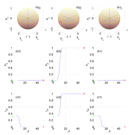
Figure 1: Time evolution for $\left|\psi_{\mathrm{i}}\right\rangle\simeq\left|\psi_{\mathrm{GHZ}}\right\rangle$. The initial state, which is given by $\left|\psi_{\mathrm{i}}\right\rangle\sim\left|\psi_{\mathrm{GHZ}}\right\rangle-10^{-5}i\left|\psi_{\mathrm{B},1}\left(\pi\right)\right\rangle-5.2\times 10^{-4}i\left|\psi_{\mathrm{B},2}\left(\pi\right)\right\rangle$, is represented by green star symbols, and the final state at time $t=50/\gamma$ by red star symbols.

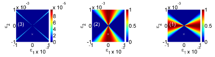
Figure 2: Partial entanglements for $\left|\psi_{\mathrm{i}}\right\rangle\sim\left|\psi_{\mathrm{GHZ}}\right\rangle+i\epsilon_{1}\left|\psi_{\mathrm{B},1}\left(\pi\right)\right\rangle+i\epsilon_{2}\left|\psi_{\mathrm{B},2}\left(\pi\right)\right\rangle$. The values of $\tau_{23}$, $\tau_{31}$, and $\tau_{12}$ at the final time $t=50/\gamma$ are shown in (1), (2) and (3), respectively, as a function of $\epsilon_{1}$ and $\epsilon_{2}$. The overlaid white $\times$ symbol represents the initial state $\left|\psi_{\mathrm{i}}\right\rangle$ used for generating the plots in Fig. 1.

For the example shown in Fig. 1, the initial state $\left|\psi_{\mathrm{i}}\right\rangle$ is given by $\left|\psi_{\mathrm{i}}\right\rangle\sim\left|\psi_{\mathrm{GHZ}}\right\rangle+i\epsilon_{1}\left|\psi_{\mathrm{B},1}\left(\pi\right)\right\rangle+i\epsilon_{2}\left|\psi_{\mathrm{B},2}\left(\pi\right)\right\rangle$, where $\epsilon_{1}=-10^{-5}$ and $\epsilon_{2}=-5.2\times 10^{-4}$. The symbol $\sim$ stands for equality up to normalization, i.e. $\left|\psi_{\mathrm{i}}\right\rangle\sim\left|\psi^{\prime}\right\rangle$ implies that $\left|\psi_{\mathrm{i}}\right\rangle=\left|\psi^{\prime}\right\rangle/\left\|\left|\psi^{\prime}\right\rangle\right\|$. The states $\left|\psi_{\mathrm{B},n}\left(\theta\right)\right\rangle$, where $n\in\left\{1,2,3\right\}$, and where $\theta$ is real, are two-spin Bell states given by

$$\left|\psi_{\mathrm{B},1}\left(\theta\right)\right\rangle =\frac{\left|000\right\rangle+e^{i\theta}\left|110\right\rangle}{\sqrt{2}}\;,$$ (6)

$$\left|\psi_{\mathrm{B},2}\left(\theta\right)\right\rangle =\frac{\left|000\right\rangle+e^{i\theta}\left|101\right\rangle}{\sqrt{2}}\;,$$ (7)

$$\left|\psi_{\mathrm{B},3}\left(\theta\right)\right\rangle =\frac{\left|000\right\rangle+e^{i\theta}\left|011\right\rangle}{\sqrt{2}}\;.$$ (8)

The overlaid white $\times$ symbol in Fig. 2 represents the initial state $\left|\psi_{\mathrm{i}}\right\rangle$ used for generating the plots in Fig. 1. For this initial state $\left|\psi_{\mathrm{i}}\right\rangle$, the final state $\left|\psi_{\mathrm{f}}\right\rangle$ is approximately $\left|\psi_{\mathrm{f}}\right\rangle\simeq\left(1/2\right)\left(\left|000\right\rangle+i\left|010\right\rangle+i\left|101\right\rangle-\left|111\right\rangle\right)$. The values of the partial entanglements $\tau_{23}$, $\tau_{31}$, and $\tau_{12}$ at the final time $t=50/\gamma$ are shown in Fig. 2 (1), (2) and (3), respectively, as a function of $\epsilon_{1}$ and $\epsilon_{2}$.

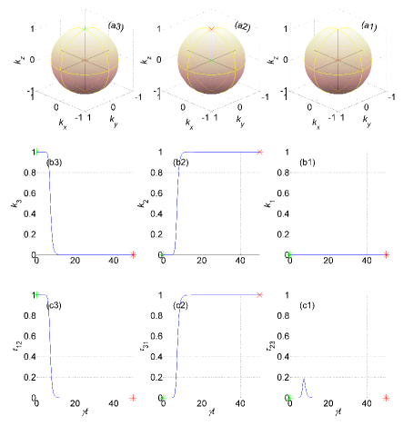
Figure 3: Time evolution for $\left|\psi_{\mathrm{i}}\right\rangle\simeq\left|\psi_{\mathrm{B},3}\left(\pi\right)\right\rangle$. The initial state, which is given by $\left|\psi_{\mathrm{i}}\right\rangle\sim\left|\psi_{\mathrm{B},3}\left(\pi\right)\right\rangle+9\times 10^{-5}i\left|\psi_{\mathrm{B},2}\left(\pi\right)\right\rangle$, is represented by green star symbols, and the final state at time $t=50/\gamma$ by red star symbols.

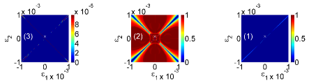
Figure 4: Partial entanglements for $\left|\psi_{\mathrm{i}}\right\rangle\sim\left|\psi_{\mathrm{B},3}\left(\pi\right)\right\rangle+i\epsilon_{1}\left|\psi_{\mathrm{B},1}\left(\pi\right)\right\rangle+i\epsilon_{2}\left|\psi_{\mathrm{B},2}\left(\pi\right)\right\rangle$. The values of $\tau_{23}$, $\tau_{31}$, and $\tau_{12}$ at the final time $t=50/\gamma$ are shown in (1), (2) and (3), respectively, as a function of $\epsilon_{1}$ and $\epsilon_{2}$. The overlaid white $\times$ symbol represents the initial state $\left|\psi_{\mathrm{i}}\right\rangle$ used for generating the plots in Fig. 3.

As is demonstrated by Fig. 1(c3) and Fig. 3(c3), generically, $\tau_{12}\rightarrow 0$ in the limit $t\rightarrow\infty$, due to the partial disentanglement generated by the term proportional to $\mathcal{Q}_{12}-\left\langle\mathcal{Q}_{12}\right\rangle$ in Eq. (1). The set $V_{n}\subset H$ is a subset of the Hilbert space $H=H_{3}\otimes H_{2}\otimes H_{1}$ containing all state vectors $\left|\psi\right\rangle\in H$, for which $k_{n}=1$, where $n\in\left\{1,2,3\right\}$, i.e. the $n$’th spin is fully separable for all $\left|\psi\right\rangle\in V_{n}$. Note that $V_{1}\cap V_{2}=V_{2}\cap V_{3}=V_{3}\cap V_{1}$ is the set of fully disentangled states (i.e. $k_{1}=k_{2}=k_{3}=1$), which is denoted by $V$. Let $\left|\psi_{\infty}\right\rangle$ be the solution of Eq. (1) in the limit $t\rightarrow\infty$, for which $\tau_{12}=0$ (i.e. entanglement between spin 1 and spin 2 vanishes). Generically, either $\left|\psi_{\infty}\right\rangle\subset V_{1}$ (for this case $k_{1}=1$, $k_{2}=k_{3}\leq 1$, $\tau_{12}=\tau_{31}=0$, and $\tau_{23}\geq 0$ ), or $\left|\psi_{\infty}\right\rangle\subset V_{2}$ (for this case $k_{2}=1$, $k_{3}=k_{1}\leq 1$, $\tau_{12}=\tau_{23}=0$, and $\tau_{31}\geq 0$). Note that $\left|\psi_{\infty}\right\rangle\subset V_{2}$ for both examples shown in Fig. 1 and in Fig. 3. For the general case, the entire Hilbert space $H$ is divided into two basins of attraction, $B_{1}$ and $B_{2}$. The basin $B_{n}$ is the set of all initial states $\left|\psi_{\mathrm{i}}\right\rangle\in H$, for which in the limit $t\rightarrow\infty$ the final state $\left|\psi_{\infty}\right\rangle\subset V_{n}$, i.e. $k_{n}=1$, where $n\in\left\{1,2\right\}$.

As can be seen from Fig. 2, the GHZ state vector $\left|\psi_{\mathrm{GHZ}}\right\rangle$ lies on the separatrix between the basins of attraction $B_{1}$ and $B_{2}$. The strong dependency of $\left|\psi_{\infty}\right\rangle$ on the initial state $\left|\psi_{\mathrm{i}}\right\rangle$, which becomes extreme in the vicinity of $\left|\psi_{\mathrm{GHZ}}\right\rangle$, resembles the butterfly effect. As is demonstrated below in Fig. 4, a similar butterfly effect occurs near the state vector $\left|\psi_{\mathrm{B},3}\left(\pi\right)\right\rangle$.

For the plots shown in Fig. 3 and Fig. 4 , the initial state vector $\left|\psi_{\mathrm{i}}\right\rangle$ is given by $\left|\psi_{\mathrm{i}}\right\rangle\sim\left|\psi_{\mathrm{B},3}\left(\pi\right)\right\rangle+i\epsilon_{1}\left|\psi_{\mathrm{B},1}\left(\pi\right)\right\rangle+i\epsilon_{2}\left|\psi_{\mathrm{B},2}\left(\pi\right)\right\rangle$. For the example shown in Fig. 3, $\epsilon_{1}=0$ and $\epsilon_{2}=9\times 10^{-5}$. This initial state is indicated by the white $\times$ symbol in Fig. 4. The corresponding final state $\left|\psi_{\mathrm{f}}\right\rangle$ is approximately $\left|\psi_{\mathrm{f}}\right\rangle\simeq\left|\psi_{\mathrm{B},2}\left(-\pi/2\right)\right\rangle$. As can be seen from Fig. 4, the butterfly effect occurs near the state $\left|\psi_{\mathrm{B},3}\left(\pi\right)\right\rangle$, which also (as the state $\left|\psi_{\mathrm{GHZ}}\right\rangle$) lies on the separatrix between the basins of attraction $B_{1}$ and $B_{2}$.

Summary - The proposed modified Schrödinger equation (1) demonstrates a way to extend quantum mechanics to enable processes of deterministic partial disentanglement in a multipartite system. Conflicts with both principles of causality and separability can be avoided by postulating that partial disentanglement between two given subsystems is active only during the time when they interact Buks_2303_00697 . This assumption of local disentanglement implies that the disentanglement rate $\gamma$ in Eq. (1) vanishes during the time when subsystems are decoupled. Further theoretical study is needed to determine whether quantum mechanics can be self-consistently reformulated based on deterministic dynamics. Alternative theoretical models for the process of quantum measurement can be experimentally tested Buks_014421 .

Acknowledgments - A useful discussion with Eliahu Cohen is acknowledged. This work was supported by the Israeli science foundation, and the Israeli ministry of science.

Appendix A The function $\tau\left(\left|\psi\right\rangle\right)$

For a given Hermitian operator $\mathcal{Q}=\mathcal{Q}^{{\dagger}}$, the function $\tau\left(\left|\psi\right\rangle\right)$, which maps a ket vector $\left|\psi\right\rangle$ to a real number $\tau$, is defined by

$$\tau\left(\left|\psi\right\rangle\right)\equiv\frac{\left\langle\psi\right|\mathcal{Q}\left|\psi\right\rangle}{\left\langle\psi\right.\left|\psi\right\rangle}\;.$$ (9)

Let $\Delta_{\tau}=\tau\left(\left|\psi\right\rangle+\epsilon\left|\delta\right\rangle\right)-\tau\left(\left|\psi\right\rangle\right)$, where $\epsilon$ is real, and $\left|\delta\right\rangle$ is a ket vector. For $\left\langle\psi\right.\left|\psi\right\rangle=1$ the following holds $\Delta_{\tau}=2\epsilon\operatorname{Re}\left\langle\delta\right.\left|q_{\psi}\right\rangle+O\left(\epsilon^{2}\right)$, where $\left|q_{\psi}\right\rangle=\left(\mathcal{Q}-\left\langle\psi\right|\mathcal{Q}\left|\psi\right\rangle\right)\left|\psi\right\rangle$. Within the set of normalized ket vectors, the term $\operatorname{Re}\left\langle\delta\right.\left|q_{\psi}\right\rangle$ is maximized for $\left|\delta\right\rangle=\left|q_{\psi}\right\rangle/\sqrt{\left\langle q_{\psi}\right.\left|q_{\psi}\right\rangle}$. Moreover, $\left\langle\psi\right.\left|q_{\psi}\right\rangle=0$ provided that $\left\langle\psi\right.\left|\psi\right\rangle=1$. Based on these observations, the nonlinear term added to the Schrödinger equation (1) is chosen to be proportional to $\left|q_{\psi}\right\rangle$.

References

- (1) E. Schrodinger, “Die gegenwartige situation in der quantenmechanik”, Naturwissenschaften, vol. 23, pp. 807, 1935.
- (2) Roger Penrose, “Uncertainty in quantum mechanics: faith or fantasy?”, Philosophical Transactions of the Royal Society A: Mathematical, Physical and Engineering Sciences, vol. 369, no. 1956, pp. 4864–4890, 2011.
- (3) A. J. Leggett, “Experimental approaches to the quantum measurement paradox”, Found. Phys., vol. 18, pp. 939–952, 1988.
- (4) A. J. Leggett, “Realism and the physical world”, Rep. Prog. Phys., vol. 71, pp. 022001, 2008.
- (5) Michael R Geller, “Fast quantum state discrimination with nonlinear ptp channels”, arXiv:2111.05977, 2021.
- (6) Steven Weinberg, “Testing quantum mechanics”, Annals of Physics, vol. 194, no. 2, pp. 336–386, 1989.
- (7) Steven Weinberg, “Precision tests of quantum mechanics”, in THE OSKAR KLEIN MEMORIAL LECTURES 1988–1999, pp. 61–68. World Scientific, 2014.
- (8) H-D Doebner and Gerald A Goldin, “On a general nonlinear schrödinger equation admitting diffusion currents”, Physics Letters A, vol. 162, no. 5, pp. 397–401, 1992.
- (9) H-D Doebner and Gerald A Goldin, “Introducing nonlinear gauge transformations in a family of nonlinear schrödinger equations”, Physical Review A, vol. 54, no. 5, pp. 3764, 1996.
- (10) Nicolas Gisin and Ian C Percival, “The quantum-state diffusion model applied to open systems”, Journal of Physics A: Mathematical and General, vol. 25, no. 21, pp. 5677, 1992.
- (11) David E Kaplan and Surjeet Rajendran, “Causal framework for nonlinear quantum mechanics”, Physical Review D, vol. 105, no. 5, pp. 055002, 2022.
- (12) Manuel H Muñoz-Arias, Pablo M Poggi, Poul S Jessen, and Ivan H Deutsch, “Simulating nonlinear dynamics of collective spins via quantum measurement and feedback”, Physical review letters, vol. 124, no. 11, pp. 110503, 2020.
- (13) Angelo Bassi, Kinjalk Lochan, Seema Satin, Tejinder P Singh, and Hendrik Ulbricht, “Models of wave-function collapse, underlying theories, and experimental tests”, Reviews of Modern Physics, vol. 85, no. 2, pp. 471, 2013.
- (14) Philip Pearle, “Reduction of the state vector by a nonlinear schrödinger equation”, Physical Review D, vol. 13, no. 4, pp. 857, 1976.
- (15) Gian Carlo Ghirardi, Alberto Rimini, and Tullio Weber, “Unified dynamics for microscopic and macroscopic systems”, Physical review D, vol. 34, no. 2, pp. 470, 1986.
- (16) Angelo Bassi and GianCarlo Ghirardi, “Dynamical reduction models”, Physics Reports, vol. 379, no. 5-6, pp. 257–426, 2003.
- (17) Charles H Bennett, Debbie Leung, Graeme Smith, and John A Smolin, “Can closed timelike curves or nonlinear quantum mechanics improve quantum state discrimination or help solve hard problems?”, Physical review letters, vol. 103, no. 17, pp. 170502, 2009.
- (18) Krzysztof Kowalski, “Linear and integrable nonlinear evolution of the qutrit”, Quantum Information Processing, vol. 19, no. 5, pp. 1–31, 2020.
- (19) Bernd Fernengel and Barbara Drossel, “Bifurcations and chaos in nonlinear lindblad equations”, Journal of Physics A: Mathematical and Theoretical, vol. 53, no. 38, pp. 385701, 2020.
- (20) K Kowalski and J Rembieliński, “Integrable nonlinear evolution of the qubit”, Annals of Physics, vol. 411, pp. 167955, 2019.
- (21) Angelo Bassi and Kasra Hejazi, “No-faster-than-light-signaling implies linear evolution. a re-derivation”, European Journal of Physics, vol. 36, no. 5, pp. 055027, 2015.
- (22) Thomas F. Jordan, “Assumptions that imply quantum dynamics is linear”, Phys. Rev. A, vol. 73, pp. 022101, Feb 2006.
- (23) Joseph Polchinski, “Weinberg?s nonlinear quantum mechanics and the einstein-podolsky-rosen paradox”, Physical Review Letters, vol. 66, no. 4, pp. 397, 1991.
- (24) Bassam Helou and Yanbei Chen, “Extensions of born?s rule to non-linear quantum mechanics, some of which do not imply superluminal communication”, in Journal of Physics: Conference Series. IOP Publishing, 2017, vol. 880, p. 012021.
- (25) Jakub Rembieliński and Paweł Caban, “Nonlinear evolution and signaling”, Physical Review Research, vol. 2, no. 1, pp. 012027, 2020.
- (26) Jakub Rembieliński and Paweł Caban, “Nonlinear extension of the quantum dynamical semigroup”, Quantum, vol. 5, pp. 420, 2021.
- (27) Zakarias Laberg Hejlesen, “Nonlinear quantum mechanics”, Master’s thesis, 2019.
- (28) Thomas F Jordan, “Why quantum dynamics is linear”, in Journal of Physics: Conference Series. IOP Publishing, 2009, vol. 196, p. 012010.
- (29) Eyal Buks, “Spontaneous collapse by entanglement suppression”, arXiv:2303.00697, 2023.
- (30) Jürgen Schlienz and Günter Mahler, “Description of entanglement”, Physical Review A, vol. 52, no. 6, pp. 4396, 1995.
- (31) Asher Peres, “Separability criterion for density matrices”, Physical Review Letters, vol. 77, no. 8, pp. 1413, 1996.
- (32) Sam A Hill and William K Wootters, “Entanglement of a pair of quantum bits”, Physical review letters, vol. 78, no. 26, pp. 5022, 1997.
- (33) William K Wootters, “Quantum entanglement as a quantifiable resource”, Philosophical Transactions of the Royal Society of London. Series A: Mathematical, Physical and Engineering Sciences, vol. 356, no. 1743, pp. 1717–1731, 1998.
- (34) Valerie Coffman, Joydip Kundu, and William K Wootters, “Distributed entanglement”, Physical Review A, vol. 61, no. 5, pp. 052306, 2000.
- (35) Vlatko Vedral, Martin B Plenio, Michael A Rippin, and Peter L Knight, “Quantifying entanglement”, Physical Review Letters, vol. 78, no. 12, pp. 2275, 1997.
- (36) Christopher Eltschka and Jens Siewert, “Quantifying entanglement resources”, Journal of Physics A: Mathematical and Theoretical, vol. 47, no. 42, pp. 424005, 2014.
- (37) Wolfgang Dür, Guifre Vidal, and J Ignacio Cirac, “Three qubits can be entangled in two inequivalent ways”, Physical Review A, vol. 62, no. 6, pp. 062314, 2000.
- (38) Xavier Coiteux-Roy, Elie Wolfe, and Marc-Olivier Renou, “No bipartite-nonlocal causal theory can explain nature?s correlations”, Physical review letters, vol. 127, no. 20, pp. 200401, 2021.
- (39) Evangelia Takou, Edwin Barnes, and Sophia E Economou, “Precise control of entanglement in multinuclear spin registers coupled to defects”, Physical Review X, vol. 13, no. 1, pp. 011004, 2023.
- (40) Andreas Elben, Richard Kueng, Hsin-Yuan Robert Huang, Rick van Bijnen, Christian Kokail, Marcello Dalmonte, Pasquale Calabrese, Barbara Kraus, John Preskill, Peter Zoller, et al., “Mixed-state entanglement from local randomized measurements”, Physical Review Letters, vol. 125, no. 20, pp. 200501, 2020.
- (41) Eyal Buks, Quantum mechanics - Lecture Notes, http://buks.net.technion.ac.il/teaching/, 2023.
- (42) Daniel M Greenberger, Michael A Horne, and Anton Zeilinger, “Going beyond bell?s theorem”, Bell?s theorem, quantum theory and conceptions of the universe, pp. 69–72, 1989.
- (43) Eyal Buks and Banoj Kumar Nayak, “Quantum measurement with recycled photons”, Physical Review B, vol. 105, no. 1, pp. 014421, 2022.