Domain-Agnostic Batch Bayesian Optimization with Diverse Constraints via Bayesian Quadrature

Abstract

Real-world optimisation problems often feature complex combinations of (1) diverse constraints, (2) discrete and mixed spaces, and are (3) highly parallelisable. (4) There are also cases where the objective function cannot be queried if unknown constraints are not satisfied, e.g. in drug discovery, safety on animal experiments (unknown constraints) must be established before human clinical trials (querying objective function) may proceed. However, most existing works target each of the above three problems in isolation and do not consider (4) unknown constraints with query rejection. For problems with diverse constraints and/or unconventional input spaces, it is difficult to apply these techniques as they are often mutually incompatible. We propose cSOBER, a domain-agnostic prudent parallel active sampler for Bayesian optimisation, based on SOBER of Adachi et al. (2023). We consider infeasibility under unknown constraints as a type of integration error that we can estimate. We propose a theoretically-driven approach that propagates such error as a tolerance in the quadrature precision that automatically balances exploitation and exploration with the expected rejection rate. Moreover, our method flexibly accommodates diverse constraints and/or discrete and mixed spaces via adaptive tolerance, including conventional zero-risk cases. We show that cSOBER outperforms competitive baselines on diverse real-world blackbox-constrained problems, including safety-constrained drug discovery, and human-relationship-aware team optimisation over graph-structured space.

1 Introduction

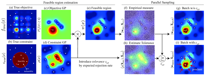
Figure 1: cSOBER algorithm. We wish to find the global maximum of (a) true objective $f_{\text{true}}$, but we have unknown (b) true constraint $c_{\text{true}}$ (feasible region shaded red). Only 5 out of 15 initial observations (white dots) met the constraints, then unsatisfying points are rejected. We place (c) objective GP (LFI; $P(f(x)\geq\eta)$) and (d) constraint GP (the probability of acceptance $\rho$). The product of both objective and constraint feasible regions yields the total (e) feasible region $\pi$. In the original SOBER procedure, they sample (f) the empirical measure $(\textbf{w}_{\text{rec}},\textbf{X}_{\text{rec}})$ based on $\pi$, then RCHQ subsamples a reduced measure $(\textbf{w}_{\text{batch}},\textbf{X}_{\text{batch}})$ as (g) batch acquisition (green dots are the selected locations). This procedure does not consider the precision requirement. So we further estimate (h) the tolerance $\epsilon_{\text{LP}}$ as the expected rejection rate using empirical measure and acceptance probability $\rho$. We propagate this estimated tolerance $\epsilon_{\text{LP}}$ as a lower precision requirement to the quadrature solver as the threshold of the inequality constraint. As a result, (i) the batch samples are now more prudent and are more likely to satisfy the unknown constraints.

Bayesian optimisation (BO) [24] is a successful blackbox optimiser for a variety of applications, e.g. drug discovery [26, 31], materials [1], and hyperparameter optimisation [21, 93] To extend applicability and flexibility, many BO variants have been proposed. For instance, (1) constrained BO for global optimisation under diverse constraints [23, 25, 41, 42, 56, 20]; (2) discrete and mixed input space BO for global optimisation over combinatorial, ordinal or mixed spaces [89, 8, 68, 79, 17, 16, 86], and (3) batch acquisition offers parallel querying for faster wall-clock speed [6, 27, 44, 51, 50, 19, 2]. This paper investigates the problems combining all the above three extensions, which can not be done efficiently with a naïve combination of existing methods, because many approaches feature incompatible and bespoke components. In addition, we consider (4) the unknown constraints where the objective function cannot be queried if unknown constraints are not satisfied, which is not previously researched.

Motivation for Domain-Agnostic Batch BO with Diverse Constraints. Unlike an academic setting where we may study the different constraints and design options (e.g. scaling to large batches) in isolation, real-life problems can be much more complicated: for example, they may have multiple types of constraints at the same time (Table 1 represents diverse constraints), while still requiring large batch suggestions (e.g. 384 experiments in parallel [11]). Furthermore, the optimisation target is often on discrete and non-Euclidean spaces (e.g. graphs, molecules), and the constraints in real life can also be unknown. We considered diverse real-world situations where these complex combinations naturally appear (see Section 5 for details, a prime example is safety-constrained drug discovery).

Challenges in Constrained Bayesian Optimisation. Existing works largely fall short in addressing these multifaceted issues: existing BO methods are not compatible with combining the above three problems, and do not address (4) the ordered constraints (see Table 1 for the definition). For instance, COMBO [68] proposed a global optimisation method over discrete space via a graph Cartesian kernel. When applied to the similarly-discrete space of molecules, this kernel is not compatible with Tanimoto kernel [74], which is popular in drug discovery [31]. Most recent works rely on special kernels or acquisition functions (AFs) tailored for specific targets, thus similarly hard to combine. Moreover, the ordered constraint causes significant information loss but no existing work treats this risk separately under unknown constraints. As Figure 1 demonstrated, 10 of 15 samples are rejected by unknown constraints. The Gaussian process (GP) has to estimate the objective with little knowledge of only 5 samples, which is significantly disadvantageous relative to the case in which it can gather all. We need to adaptively balance exploitation and exploration according to a dynamically-changing level of rejection risk. However, most existing constrained approaches do not distinguish between ordered and unordered cases. For instance, PESC [41] proposed information-theoretic AF-based constrained BO. However, the acquisition principle is solely information gain; querying the most informative points. Yet, rejections and, hence, no information gain are much worse than querying less informative but safe locations to secure sure information gain in total. Thus, this does not consider changing the level of penalising exploration under rejection risk (we refer to prudence). Moreover, existing BO techniques fall short in the large batch and discrete/mixed search space due to expensive computation or combinatorial explosion (see [2] for details).

Table 1: Definitions of diverse unknown constraints appeared in Bayesian optimisation literature. Our approach is capable of handling all these constraint types and/or a combination of them.

	cases	definitions
constraints on querying	coupled [25]	Both objective and constraints are queried together.
	decoupled [43]	Objectives and constraints are queried separately.
	ordered [71]	The objective can be queried only if queried constraints are satisfied.
	unordered [25]	The objective can be queried regardless of constraints satisfaction.
	cheap [23]	A querying cost of constraints is negligibly cheap.
	expensive [25]	Querying constraints is expensive to evaluate.
outcome types	deterministic [23]	The feedback from constraints is always true.
	probabilistic [25]	The feedback is noisy values or in form of probability distribution.
	binary [25]	The feedback from constraints are binary (true or false).
	continuous [23]	The feedback is continuous latent values judging constraint satisfaction.

Contribution. Amongst the existing methods, we find SOBER [2] has a number of advantages making it a suitable candidate to address the complicated problems we have. However, SOBER does not consider constraints, particularly challenging in the ordered case due to its explorative nature. The main contributions of this work are as follows:

1. We propose constrained SOBER (cSOBER), the first algorithm to achieve both BO with scalable batching over a general input space under any constraints in Table 1.

2. cSOBER is modular and model-agnostic, and can be easily combined with existing BO methods in a blackbox manner for arbitrary AFs and kernel.

3. We derived a theoretical analysis of kernel quadrature under ordered constraints.

4. cSOBER showed a strong empirical performance over diverse real-world optimisation tasks.

2 Related Work and Challenges

2.1 Constrained Batch Bayesian Optimisation

Table 2: Comparison of constrained batch global optimisation algorithms. See Table 1 for definitions of decoupled, cheap, blackbox, and ordered. Only cSOBER can handle all features simultaneously.

	blackbox constraints			customisability		compatibility
baselines	decoupled?	ordered?	cheap?	AFs?	kernels?	scalable batching?	Non- Euclidean?
cEI [56]	✕	✕	✕	✕	✓	✓	✕
PESC [42]	✓	✕	✕	✕	✓	✕	✕
SCBO [20]	✕	✕	✓	✕	✕	✓	✕
PropertyDAG [71]	✕	✕	✕	✕	✓	✕	✕
cTS [44, 20]	✕	✕	✓	✕	✓	✓	✓
VAE-BO [61, 67]	N/A for unknown constraints			✓	✓	✕	✓
cSOBER (Ours)	✓	✓	✓	✓	✓	✓	✓

BO has gained enormous popularity and has a long parade of existing approaches, so we focus on the methods that can deal with (1) constraints, (2) non-Euclidean space, and (3) massively parallelisable optimisation. (See Supplements for the primer on BO and GP). Table 2 summarises the key differences with competitive baselines. Popular methods (cEI [56], PESC [42], PropertyDAG [71], cTS [44, 20]) rely on specific AFs. SCBO [20] rely on specific kernels to define trust regions. Constrained optimisation in the non-Euclidean setup has not been thoroughly studied. For instance, popular variational autoencoder (VAE)-based BO methods, such as LOL-BO [61], need pretraining on unlabelled data, which is not always available, to define latent spaces. Furthermore, the constraints in the context ofVAE BO may constrain the VAE to generate more realistic molecules or images under explicit and known constraints, but are not capable of handling or estimating unknown constraints. Since we target black-box constraints, we do not compare with vanilla BO. PropertyDAG [71] handles ordered constraints by explicitly modelling underlying known constraints to the surrogate model but cannot handle unknown constraints. Thus, our method cSOBER is the only method that can deal with arbitrary AFs and arbitrary kernels over discrete and mixed spaces under arbitrary constraints in Table 1 (See details in Suppl. C).

2.2 SOBER: Solving Global Optimisation as Quadrature

SOBER is the first algorithm to bridge BO and Bayesian quadrature (BQ). BQ [69, 39] is a model-based blackbox integration method akin to BO, both under the umbrella of probabilistic numerics (PN) [39]. SOBER re-framed batch BO as batch BQ via the following dual objective of global optimisation:

$$x^{*}_{\text{true}}\in\arg\max_{x}f_{\text{true}}(x)\quad\xLeftrightarrow{\text{dual}}\quad\delta_{x^{*}_{\text{true}}}\in\mathop{\mathrm{missing}}{arg\,max}_{\pi}\int f_{\text{true}}(x)\text{d}\pi(x),$$ (1)

where $f_{\text{true}}$ is the true blackbox objective function, $x^{*}_{\text{true}}$ is the location of the global maximum, $\pi$ is a probability distribution over the feasible region, and $\delta_{x}$ is the delta distribution at $x$. Namely, this explains the equivalence between finding the global maximum of the blackbox function $x^{*}_{\text{true}}$ and finding the delta distribution at the global maximum $x^{*}_{\text{true}}$. This dual objective casts BO as BQ, as Eq. (1) is an integration problem. SOBER adopts the BASQ framework [3, 4] for solving batch BQ, thus SOBER inherits the known benefits of BASQ in batch BO, such as generality in modelling and supports large batches. SOBER updates $\pi$ until it becomes a delta distribution (a set of delta functions in a multiple global optimal case). SOBER samples $x$ from an arbitrary (continuous or discrete) probability distribution $\pi$ and thus may be applied in an arbitrary input space. RCHQ is a subsample-based, gradient-free solver with the only requirement being that the input variables $x$ can easily be sampled from $\pi$. This is ideal for non-Euclidean and discrete spaces such as molecules or graphs because it is difficult to apply typical gradient-based methods used in BO for optimising AFs in these spaces, but sampling candidates is simple. Furthermore, RCHQ is provably sample-efficient: it minimises the total predictive uncertainty under a given probability measure $\pi$ . Moreover, SOBER can solve BQ tasks, such as simulation-based inference, via dual GP (see Suppl. C in [2].)

Nonetheless, the original SOBER does not support constraints. As the AF term in SOBER is a penalty term, it is possible for the algorithm to suggest an infeasible location even if the AF itself is constrained. This is mainly because SOBER is a quadrature algorithm, so the first priority in batch selection is the minimisation of worst-case integration error rather than satisfying constraints. The recombination constraints with test functions (equality constraints) are more prioritised than acquisition function maximisation (penalty term). Therefore, SOBER with hard constraints cannot be done by a naïve combination.

3 Proposed Method: cSOBER

Now, we present cSOBER, built upon SOBER to be applicable to all combinations of constraints in Table 1 while maintaining the generality to large batch BO and BQ over discrete and mixed spaces. Figure 1 summarises the overview of cSOBER algorithm (see algorithm flow in Suppl. E). In particular, the key differences from SOBER are the ability to handle constrained BOs and the introduction of tolerance in the quadrature solver (the importance is analyised in §4 later). As Figure 1 clearly demonstrates, the tolerance allows for more prudent sampling under ordered constraints, and allows the algorithm to adaptively balance between exploitation and exploration. The core rationale of introducing tolerance is the fact that it is impossible to guarantee feasibility beforehand due to the presence of unknown ordered constraints, where (in)feasibility may only be established after actually querying the locations. In other words, this rejection risk defines the level of inevitable inaccuracy in integration; improving integration accuracy beyond the threshold does not guarantee improved sample-efficiency as a constrained global optimiser. Thus, we set the tolerance as the threshold of quadrature precision, by estimation from the expected rejection rate. This tolerance releases the additional degree of freedom to maximise the AF. When we set the acceptance probability as the penalty term of quadrature, the resulting batch samples are expected to have a larger acceptance probability, leading to more prudent sampling. Moreover, this tolerance can be estimated and changed adaptively over iterations.

Problem Definition. We start with the most general case of expensive black-box constraints (other cases may be cast as a special case of this). Probabilistic constraints are typically handled by probabilistic surrogate models, normally using GP [25]. Under the probabilistic surrogate models, the goal is to solve the following constrained measure optimisation problem:

$$\delta_{x^{*}_{\text{true}}}\in\mathop{\mathrm{missing}}{arg\,max}_{\pi}\int f_{\text{true}}(x)\text{d}\pi(x)\quad\text{s.t.}\quad\rho_{\text{true},\ell}(x)\geq\epsilon_{\ell},\,\forall\ell\in\mathbb{N}_{\leq L}$$ (2)

where $x$ is a sample drawn from $\pi$, the probability measure on the domain $\mathcal{X}$, a completely general input space, e.g., a (non-)Euclidean, discrete, graph-structured, or their mixture. $d$ is the dimension, $L$ is the number of constraints, $\rho_{\text{true},\ell}$ is the $\ell$-th true acceptance probability function $\rho:\mathcal{X}\rightarrow[0,1]$, also can be written as $\rho_{\text{true},\ell}(x):=\text{Pr}(c_{\text{true},\ell}(x))$, $c_{\text{true},\ell}$ is the $\ell$-th Boolean function indicating whether or not the constraint is satisfied $c:\mathcal{X}\rightarrow\{0,1\}$, and $\epsilon_{\ell}$ is the minimum allowable probability.

3.1 Constraining the Feasible Region $\pi$

In SOBER, while $\pi$ may be used to define the feasible region (exploitation), random convex hull quadrature (RCHQ) selects a diversified uncertain batch of samples (exploration). We constrain $\pi$ instead of constraining the AF, the former of which can be understood as rejection sampling.

Unordered constraints. Following likelihood-free inference (LFI) [34] and existing constrained BO literature [25], we define $\pi$ as:

$$\pi(x)\propto\underbrace{\Phi\left[\frac{m_{\text{obj}}(x)-\eta}{\sqrt{C_{\text{obj}}(x,x)}}\right]}_{\text{LFI}}\underbrace{\prod_{\ell=1}^{L}\max\left[\rho_{\ell}(x)-\epsilon_{\ell},0\right]}_{\text{constraints}},$$ (3)

where $\Phi$ is the standard Gaussian cumulative density function (CDF), $m_{\text{obj}}(\cdot)$ and $C_{\text{obj}}(\cdot,\cdot)$ are the predictive mean and covariance of the GP for objective, $\eta:=\max\mathbb{E}[f(x)]$ is the global maximum of the current GP for objective $f$, and $\rho_{\ell}$ is the acceptance probability function estimated from a probabilistic surrogate model of constraints (see Suppl. D). This likelihood definition is the same as the probability of improvement AF [55]. Note that $\pi$ is on the general space $\mathcal{X}$, thus $\pi$ becomes a probability mass function if $\mathcal{X}$ is discrete.

Typically as the optimisation progresses, as we find better points, $\eta_{i}$ increases and the variance $\mathbb{V}\text{ar}[\pi(x)]$ shrinks. Ideally, when there is a single global maximum, $\pi$ eventually approaches $\delta_{x^{*}_{\text{true}}}$, where $\eta_{\infty}=f_{\text{true}}(x^{*}_{\text{true}})=\mathbb{E}[f(x^{*}_{\text{true}})]$. The original SOBER [2] empirically investigated that the LFI without the constraint term has strong linear correlations between $\mathbb{V}\text{ar}[\pi(x)]$ and Bayesian regret (Theorem 2 in [50]). We observed the same tendency for cSOBER, suggesting duality in Eq. (1) is still preserved in constrained cases (see Suppl. E.).

Ordered Constraints. With the above definition of $\pi$ in Eq. (3), we further consider tolerance $\epsilon$ in the quadrature precision to achieve prudent sampling in the ordered constraints. We wish to design tolerance to be adaptive to the level of rejection risk from true constraints, we define the tolerance as the rejection rate $\epsilon_{\text{rej}}$. Nevertheless, the true rejection rate $\epsilon_{\text{true, rej}}:=1-\textbf{1}^{\top}\bigodot_{\ell=1}^{L}c_{\text{true},\ell}(\textbf{X}_{\text{batch}})/n\approx 1-\textbf{w}_{\text{batch}}^{\top}\bigodot_{\ell=1}^{L}\rho_{\text{true},\ell}(\textbf{X}_{\text{batch}})$ depends on the true constraints $c_{\text{true},\ell}$, which as discussed, are not known until we actually query the objective function; we instead estimate the rejection rate from surrogate $\rho_{\ell}$, $\epsilon_{\text{rej}}:=1-\int\bigodot_{\ell=1}^{L}\rho_{\ell}(x)\text{d}\pi(x)\approx 1-\textbf{w}_{\text{rec}}^{\top}\bigodot_{\ell=1}^{L}\rho_{\ell}(\textbf{X}_{\text{rec}})$. This is the Monte Carlo (MC) estimate of expectation of rejection rate. We use $\textbf{X}_{\text{rec}}$ instead of $\textbf{X}_{\text{batch}}$, since both $(\textbf{w}_{\text{rec}},\textbf{X}_{\text{rec}})$ and $(\textbf{w}_{\text{batch}},\textbf{X}_{\text{batch}})$ are the approximation of $\pi$, and $\textbf{X}_{\text{batch}}$ is not determined until kernel recombination (§3.2), and the rejection rate is a required argument to perform kernel recombination. We then use this expected rejection rate $\epsilon_{\text{rej}}$ as the tolerance $\epsilon$ for the quadrature solver explained for the next step. Note that since the rejection rate is estimated from the surrogate models of the constraints, the values are adaptively changed according to surrogate models.

3.2 Kernel Recombination for Ordered Constraints

As a general situation, consider we are given a kernel $K_{\text{LP}}$ on $\mathcal{X}$ and an $N$-point sample $\textbf{X}_{\text{rec}}\in\mathcal{X}^{N}$ associated with a nonnegative weight $\textbf{w}_{\text{rec}}$ with $\textbf{w}_{\text{rec}}^{\top}\boldsymbol{1}=1$. The goal is to find a weighted subset $(\textbf{w}_{\text{batch}},\textbf{X}_{\text{batch}})$ of $\textbf{X}_{\text{rec}}$, which works as a compression of the larger measure $(\textbf{w}_{\text{rec}},\textbf{X}_{\text{rec}})$. Unlike the existing setting [36, 3, 2], cSOBER additionally works under the following conditions:

• After we choose $(\textbf{w}_{\text{batch}},\textbf{X}_{\text{batch}})$, each point $x\in\textbf{X}_{\text{batch}}$ is accepted with probability $q(x)$ (and rejected w.p. $1-q(x)$); the accepted points with corresponding weights $(\tilde{\textbf{w}}_{\text{batch}},\tilde{\textbf{X}}_{\text{batch}})$ are the ones we can use for the quadrature. The probability $q:\mathcal{X}\to[0,1]$ is given.

• We are given a reward function $g:\mathcal{X}\to\mathbb{R}$, and we want to make $\tilde{\textbf{w}}_{\text{batch}}^{\top}g(\tilde{\textbf{X}}_{\text{batch}})$ as big as possible while making $(\tilde{\textbf{w}}_{\text{batch}},\tilde{\textbf{X}}_{\text{batch}})$ a good kernel quadrature.

To solve the above problem, we introduce the following linear programming (LP) problem that aims to achieve both the maximization of reward and the precision of kernel quadrature, which is given by modifying the algorithm adopted in SOBER ($n\geq 3$):

$$\begin{array}[]{rl}\underset{\textbf{w}}{\text{maximize}}&\textbf{w}^{\top}\bigl{[}g(\textbf{X}_{\text{rec}})\odot q(\textbf{X}_{\text{rec}})\bigr{]},\\ \underset{\phantom{a}}{\text{subject to}}&\bigl{\lvert}(\textbf{w}-\textbf{w}_{\text{rec}})^{\top}\varphi_{j}(\textbf{X}_{\text{rec}})\bigr{\rvert}\leq\epsilon_{\text{LP}}\sqrt{\lambda_{j}/(n-2)},\quad 1\leq j\leq n-2,\\ &(\textbf{w}-\textbf{w}_{\text{rec}})^{\top}q(\textbf{X}_{\text{rec}})\geq 0,\ \ \textbf{w}^{\top}\textbf{1}=1,\ \ \textbf{w}\geq\textbf{0},\ \ |\textbf{w}|_{0}\leq n.\end{array}$$ (7)

Here, $\epsilon_{\text{LP}}\geq 0$ is a tolerance parameter, and $(\lambda_{j},\varphi_{j})$ are given by using the singular value decomposition (SVD) of $K_{\text{LP}}(\textbf{X}_{\text{nys}},\textbf{X}_{\text{nys}})=\textbf{U}\text{diag}(\lambda_{1},\ldots,\lambda_{M})\textbf{U}^{\top}$ with $\lambda_{1}\geq\cdots\geq\lambda_{M}\geq 0$, $\textbf{U}=[u_{1},\ldots,u_{M}]$ and $\varphi_{j}=u_{j}^{\top}K_{\text{LP}}(\textbf{X}_{\text{nys}},\cdot)$, where $\textbf{X}_{\text{nys}}\in\mathcal{X}^{M}$ is another $M$-point sample.

The error estimate of kernel quadrature in the original algorithm is essentially given by the approximation error of $K_{\text{nys}}(x,y):=\sum_{j=1}^{n-2}\boldsymbol{1}_{\{\lambda_{j}>0\}}\lambda_{j}^{-1}\varphi_{j}(x)\varphi_{j}(y)\approx K_{\text{LP}}(x,y)$. Let us define the corresponding error as $\epsilon_{\text{nys}}:=\max_{x\in\textbf{X}_{\text{rec}}}\lvert K_{\text{nys}}(x,x)-K_{\text{LP}}(x,x)\rvert^{1/2}$. Although not mainly in the sup norm, error bounds for this approximation have been well studied in the literature [18, 54, 38].

Proposition 1.

Under the above setting, let $\textbf{w}_{*}$ be the optimal solution of the LP (7), and let $\textbf{X}_{\text{batch}}$ be the subset of $\textbf{X}_{\text{rec}}$, corresponding to the nonzero entries of $\textbf{w}_{*}$ (denoted by $\textbf{w}_{\text{batch}}$). Suppose that $\tilde{\textbf{X}}_{\text{batch}}$ is given by a random subset of $\textbf{X}_{\text{batch}}$, where each point $x$ is accepted with probability $q(x)$, and let $\tilde{\textbf{w}}_{\text{batch}}$ be the corresponding weights. Then, we have

$$\mathbb{E}[\tilde{\textbf{w}}_{\text{batch}}^{\top}g(\tilde{\textbf{X}}_{\text{batch}})]\geq\textbf{w}_{\text{rec}}^{\top}\bigl{[}g(\textbf{X}_{\text{rec}})\odot q(\textbf{X}_{\text{rec}})\bigr{]},$$ (8)

and, for any function $f$ in the RKHS with kernel $K_{\text{LP}}$, we have

$$\mathbb{E}\!\left[\left\lvert\tilde{\textbf{w}}_{\text{batch}}^{\top}f(\tilde{\textbf{X}}_{\text{batch}})-\textbf{w}_{\text{rec}}^{\top}f(\textbf{X}_{\text{rec}})\right\rvert\right]\leq(\epsilon_{\text{rej}}K_{\max}+2\epsilon_{\text{nys}}+\epsilon_{\text{LP}})\lVert f\rVert,$$ (9)

where $\lVert f\rVert$ is the RKHS norm of $f$, $K_{\max}:=\max_{x\in\textbf{X}_{\text{rec}}}K(x,x)^{1/2}$, and $\epsilon_{\text{rej}}:=1-\textbf{w}_{\text{rec}}^{\top}q(\textbf{x}_{\text{rec}})$ is the expected rejection rate with respect to the empirical measure given by $(\textbf{w}_{\text{rec}},\textbf{X}_{\text{rec}})$.

This proposition suggests we can have a quantitative estimate of the two tasks described in (b) at the same time; we can achieve at least the expected reward of the original batch while keeping the resulting (non-necessarily probability) measure integrating the functions in the RKHS within a proven error. Suppl. A contains the proof of Proposition 1.

In Practice. $\textbf{X}_{\text{batch}}$ and $\textbf{X}_{\text{nys}}$ are given by i.i.d. samples from $\pi$. In practice, discrete space optimisation tasks are typically given as a dataset, (e.g. a drug candidate list), then we do not need to sample as we already have it. Hence, we compute the weights $\textbf{w}_{\text{rec}}$ to reframe this case as the importance sampling from given samples. The weights can be computed by the normalising $\pi$, $\textbf{w}_{\text{rec}}=\pi(\textbf{X}_{\text{rec}})/\big{[}\pi(\textbf{X}_{\text{rec}})^{\top}\textbf{1}\big{]}$. Since $\textbf{X}_{\text{nys}}$ needs to be i.i.d. sampled, we apply deweighted sampling via resampling with inverse of $\textbf{w}_{\text{rec}}$ (See detailed sampling procedure for various input spaces in [2]). The reward function is given by $g(x):=\alpha(x)$, where $\alpha$ is the user-defined arbitrary AF, this term encourages batch samples to be biased towards high AF. The probability functions are given as $q(x):=\prod_{\ell=1}^{L}\rho_{\ell}(x)$ if probabilistic blackbox constraints, otherwise $q(x):=\prod_{\ell=1}^{L}c_{\text{true},\ell}(x)$. This encourages batch samples to be sampled from where the possibility of acceptance is high (we refer to prudent sampling). We set the kernel as the posterior predictive covariances of the objective function, $K_{\text{LP}}:=C_{\text{obj}}(x,x^{\prime})$. Furthermore, to speed up the algorithm, we can make use of the recursive recombination algorithm [58, 85, 60] instead of rigorously maximising the objective function. The extension of the algorithm is essentially the same as in SOBER, but we use an LP solver instead of SVD-based elimination at each recursive step for the introduction of tolerance and better optimisation of the objective function.

Constraints Generalisability. We note that the general framework discussed is applicable to all scenarios described in Table 1. For coupled/decoupled constraints, this is simply changing the kernel $K_{LP}$. For coupled cases, we use $K_{\text{LP}}:=C_{\text{obj}}(x,x^{\prime})$. For decoupled case, we change the kernel according to the querying target; $C_{\text{obj}}(x,x^{\prime})$ for the objective, $K_{\text{LP}}=\sum_{\ell}^{L}C_{\ell}(x,x^{\prime})$ for the constraints, where $C_{\ell}$ is the predictive covariance of $\ell$-th constraint function. Since there is no risk of constraints query rejection, we set the tolerance $\epsilon_{\text{rej}}$ to set very small fixed value ($\epsilon_{\text{rej}}=10^{-8}$), which is the same with original SOBER. Ordered/unordered constraints are explained in §3.1. In the ordered case, we propagate the estimated rejection rate $\epsilon_{\text{rej}}$ as the tolerance $\epsilon_{\text{LP}}$ in LP solver, otherwise set very small fixed value. Cheap black-box constraints can be treated identically to as white-box cases: we may replace $\rho_{\ell}$ with $c_{\text{true},\ell}$. The formulation in Eq. (3) is rejection sampling, so we can handle blackbox constraints by rejecting the samples generated from LFI terms by true non-closed-form constraint $c_{\text{true},\ell}$. Deterministic constraints can be done via setting very small noise variance $\sigma^{2}_{n}$. For binary/continuous constraints modeling, see [25] and Suppl. D for details.

Budgeted Batching. The batch sizes in cSOBER are dynamically changing. This is because the designated fixed batch size can be wasteful when the number of specified evaluations is larger than the low precision requirement according to the tolerance change. LP automatically determines the batch sizes based on the tolerance, so batch size itself can be proposed by our algorithm. When we set very large batch size as an argument, LP returns batch samples with optimal small number of samples. This is preferred for limited budget cases (e.g. computational-resource-aware hyperparameter optimisation [66]). However, most batch BO methods only treats fixed batch sizes. Hence, we fill the samples using constrained Thompson sampling (TS) [20] to meet the requested batch sizes only for the sake of comparison. We adopt hallucination [6], placing the batch samples returned from LP as fantasy samples with predictive mean from GP, to avoid resampling from similar locations from already batched. Exploitive TS complements explorative LFI (see Suppl. D.3).

4 Role of Tolerance as Balancing Exploitation and Exploration

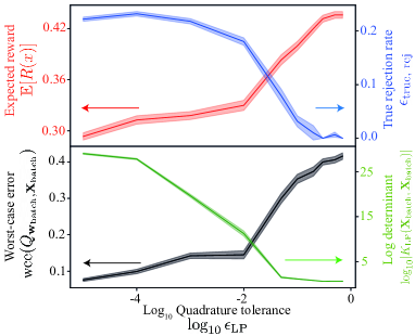
(a) Prudence vs. diversity

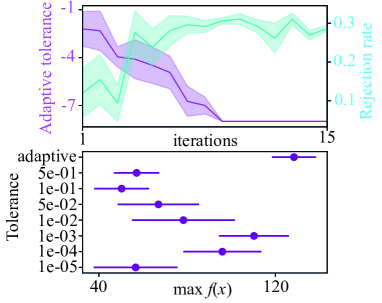
(b) Fixed vs. adaptive tolerances

Figure 2: (a) Tolerance balances between the prudence (lower rejection rate) and the diversity (log determinant). (b) Adaptive tolerance with estimated rejection rate outperforms the fixed cases.

We empirically analyse the role of tolerance in balancing exploitation and exploration. Figure 2 summarises the key results: We achieve prudent sampling via the acceptance probability: this can be evaluated by the expected reward $\mathbb{E}[R(x)]:=\tilde{\textbf{w}}_{\text{batch}}^{\top}\bigl{[}g(\tilde{\textbf{X}}_{\text{rec}})\odot q(\tilde{\textbf{X}}_{\text{rec}})\bigr{]}$. As seen in Figure 2 (a), the larger the tolerance is, the larger the expected rewards becomes, resulting in a lower true rejection rate of batch samples. Lowering quadrature precision thus releases the flexibility that allow cSOBER to find a larger expected reward to achieve prudent sampling. On the other hand, more prudent sampling is less explorative – we measure the amount of exploration as the log-determinant of the Gram matrix of batch samples $\log\lvert K(\tilde{\textbf{X}}_{\text{rec}},\tilde{\textbf{X}}_{\text{rec}})\rvert$. As the tolerance increases, the worst-case integration error increases, leading to a decrease in log determinants. This explains why the tolerance $\epsilon_{LP}$ works as a key factor in balancing the trade-off between exploitation and exploration.

We further investigate the effect of fixed and adaptive tolerances and find that a sensible strategy over iterations is discovered. Figure 2 (b) shows that adaptive tolerance converges faster than fixed tolerances in the toy, Branin function maximisation task. Moreover, we find the most effective fixed tolerance to be around $\epsilon_{\text{LP}}=10^{-3}$, rather than at the highest precision used the original SOBER; even without adaptive tolerances, this works better than original SOBER under constraints. In the adaptive case, we find the selected tolerance decreases over iterations. At the initial stage, the model is very uncertain about the constraints and the expected rejection rate is high; we argue that gathering more information with prudent sampling at this stage makes sense. Over time, the most confident regions are already explored, and the expected rejection rate is low, so we observe that the model starts to explore more outer regions. The sensible policy is automatically enabled by the adaptive tolerance as the expected rejection rate.

5 Experiments

Table 3: Experimental Setup. syn./real refers to synthetic or real-world problems, the input space of the dataset was either of Euclidean (Ecld.), discrete (Disc.), or Graph, the input represents the number of dimensions over input space of continuous (cn.), or discrete (disc.), total dimension is the summation of each dimension. Graph spaces do not have dimensions. Batch is the batch size $n$. In kernel $K$, diff. and Tani. are short for diffusion graph kernel [94] and Tanimoto kernel [74], respectively. In constraints, $L$ is the number of constraints, and other abbreviations are whether or not the dataset contains the following constraints; coupled (cp.), decoupled (dp.), ordered (o.), unordered (uo.), deterministic (dt.), probabilistic (pb.), binary (bn.), continuous (cn.), cheap (ch.), expensive (ep.) in Table 1, respectively.

input $d$

constraints

datasets

syn. /real

objective

space $\mathcal{X}$

cn.

disc.

batch $n$

kernel $K$

$L$

cp.

dp.

o.

uo.

dt.

pb.

bn.

cn.

ch.

ep.

Ackley

syn

$\log_{10}\min f$

Ecld.

3

20

200

RBF

2

✓

✓

✓

✓

✓

✓

Hartmann100

$\log_{10}\text{regret}$

Ecld.

6

-

100

RBF

2

✓

✓

✓

✓

✓

✓

Hartmann5

$\log_{10}\text{regret}$

Ecld.

6

-

5

RBF

2

✓

✓

✓

✓

✓

✓

PestControl

real

$\min f$

Disc.

-

15

200

RBF

2

✓

✓

✓

✓

✓

✓

✓

✓

Malaria

$\log_{10}\min f$

Disc.

molecule

100

Tani.

2

✓

✓

✓

✓

✓

Solvent

$-\max\log_{10}f$

Disc.

molecule

200

Tani.

3

✓

✓

✓

✓

✓

FindFixer

$\log_{10}\max f$

Graph

node

100

diff.

3

✓

✓

✓

✓

✓

✓

TeamOpt

$\log_{10}$ regret

Graph

subgraph

100

diff.

3

✓

✓

✓

✓

✓

We test the sample efficiency and sampling overhead of cSOBER against 6 baseline methods (namely, random, cEI [56], PESC [42], SCBO [20], PropertyDAG [71], for Euclidean space, cTS [44, 20] for non-Euclidean). We test upon the 8 experiments (3 synthetic and 5 real-world problems for constrained batch BO.The results are shown in Table 3 (experimental details are in Suppl. E.). Note that none of the baselines is fully compatible with all constraint types and only SOBER and cTS can handle constrained BO over non-Euclidean space, as shown in Table 2 (see Suppl. C for details). cTS has not been considered in existing work but this is a simple combination of known techniques: we adopt the two-step sampling used in SCBO to TS (the original SCBO does not apply due to kernel does not have lengthscale hyperparameter for trust region update heuristics naïvely). Other details on how baseline methods are adopted, experimental setup, and used libraries can be found in Suppl. F.

5.1 Results

Table 4: Experimental results on best objective function value (see Table 3) obtained after 15 iterations. Reported is average $\pm$ 1 standard error over 10 repeated runs. Most experiments were conducted on large batch sizes of over 100. N.Ecld. is short for non-Euclidean space.

baselines	Ackley	Hart- mann100	Hart- mann5	Pest Control	Malaria	Solvent	Find Fixer	Team Opt
Random	0.272 ± 0.01	-0.108 ± 0.03	-0.039 ± 0.05	8.582 ± 0.04	-2.381 ± 0.10	-1.015 ± 0.04	-0.908 ± 0.09	-1.647 ± 0.01
cEI	-0.002 ± 0.02	-0.218 ± 0.04	-0.065 ± 0.06	8.737 ± 0.07	Combinatorial explosion in N.Ecld.
cTS	0.234 ± 0.01	-0.577 ± 0.03	-0.550 ± 0.06	8.513 ± 0.01	-2.414 ± 0.08	1.179 ± 0.03	-0.742 ± 0.16	-0.586 ± 0.11
PESC	too slow (>7 days)		-0.090 ± 0.06	too slow	N.Ecld. and too slow (>7 days)
SCBO	0.255 ± 0.01	-0.842 ± 0.01	-1.227 ± 0.18	7.484 ± 0.13	No lengthscale in kernel for trust region and in N.Ecld.
Property DAG	-0.041 ± 0.03	-0.125 ± 0.05	-0.092 ± 0.06	8.811 ± 0.06	Combinatorial explosion in N.Ecld.
cSOBER	-3.588 ± 0.04	-1.303 ± 0.04	-1.276 ± 0.08	7.070 ± 0.00	-2.466 ± 0.08	1.199 ± 0.00	-0.195 ± 0.00	-1.895 ± 0.01

Table 4 shows that cSOBER is the top-performing of 8 both synthetic and real-world tasks we consider. Only cSOBER and cTS can handle all the problems in diverse search spaces under diverse constraints. Particularly, cSOBER outperforms the baselines significantly on the Ackley problem: the unconstrained version of this problem is also considered in the original SOBER ($-2.180\pm 0.01$). Namely, cSOBER substantially improves the convergence rate over the original SOBER by incorporating the constraint information to focus on the feasible region – constraints in this case actually helps in finding the global maximum, as the feasible regions are much smaller than the unconstrained case. Interestingly, the baselines without considering constraints (random, TS for cTS, and TurBO for SCBO) do not show such a big improvement, or perform even worse (values from in [2], $0.232\pm 0.01$ for random, $0.093\pm 0.01$ for TS, and $0.200\pm 0.01$ for TurBO). While most experiments were conducted on large batch sizes of over 100, existing methods, especially PESC, produce prohibitive overhead. We therefore prepare the low-batch size (5) experiments (Hartmann5), and find cSOBER still outperforms. When compared to the experiment with batch size of 100 (Hartmann100), surprisingly, most methods have a negligible improvement in performance even though there is a 20-fold information gain in each iteration; SCBO even performs worse with a larger batch size. In contrast, cSOBER does not suffer from these issues because of diversified sampling via quadrature. A similar trend was found in the original SOBER.

cSOBER also outperforms baselines in real-world problems over combinatorial, non-Euclidean, graph-structured spaces, where all baselines except cTS cannot be applied. Results on safety-constrained drug discovery and relationship-aware human relational graph optimisation tasks further exemplify how cSOBER handles complex real-world tasks efficiently.

6 Discussion

We introduced a versatile approach, cSOBER, capable of (1) diverse constraints, (2) discrete and mixed space, and (3) highly parallelisable global optimisation methods under (4) ordered constraints with a prudent sampler via tolerance introduction. Adaptive tolerance based on expected rejection rate plays a key role to adaptively balance between exploitation and exploration, which showed improved performance over fixed tolerance or original SOBER. The flexibility of cSOBER allows for handling complex real-life constrained optimisation problems. Moreover, cSOBER is model-agnostic, so users can augment their existing or potentially new models with bespoke AFs and kernels upon cSOBER by just changing the parallel sampling solver. In fact, most baseline methods we selected are also compatible with cSOBER (e.g. cEI is just AF definition and we can use it in cSOBER). The combination of existing works should augment both potentials.

Although we have tried to incorporate as many constraints as possible to show generalisability, there may be constraint conditions we missed in the literature. However, regarding the fact that most BO approaches are based on clever modelling of GP or AFs rather than changing the solver, such approaches should be compatible with model-agnostic cSOBER. Also, cSOBER is limited to batch setting with batch size larger than 3. We emphasise that batching over 100 queries in parallel is harder than sequentially querying, and batching can be better than the sequential setting through the lens of nonmyopic BO, such as GLASSES [28]. Our method is based on SOBER, so its limitations are inherited, namely no compatibility with asynchronised and distributed batch settings such as in [44]. Applicability to high-dimensional BO is also an open problem as efficient sampling from the posterior over the maximiser is not always available. However, sample-ready embeddings, such as linear embeddings, VAEs, and normalising flows, can make this sampling efficient. Lastly, the reason subsample-based kernel quadrature works surprisingly well in practice rather than theory has not been fully understood. Random convex hulls and hypercontractivity [35, 37] explain it in a slightly different setting. Further theoretical analysis will give a better understanding and improvement.

Appendix A Proof of Proposition 1

Proof of Proposition 1.

Note that the constraint $\lvert\textbf{w}\rvert_{0}\leq n$ is automatically satisfied when we use the simplex method or its variant. Without this constraint, we have a trivial feasible solution $\textbf{w}=\textbf{w}_{\text{rec}}$, so, for the optimal solution $\textbf{w}_{*}$, we have $\textbf{w}_{*}^{\top}\bigl{[}g(\textbf{X}_{\text{rec}})\odot q(\textbf{X}_{\text{rec}})\bigr{]}\geq\textbf{w}_{\text{rec}}^{\top}\bigl{[}g(\textbf{X}_{\text{rec}})\odot q(\textbf{X}_{\text{rec}})\bigr{]}$. Since $\mathbb{E}[\tilde{\textbf{w}}_{\text{batch}}^{\top}g(\tilde{\textbf{X}}_{\text{batch}})]=\textbf{w}_{\text{batch}}^{\top}\bigl{[}g(\textbf{X}_{\text{batch}})\odot q(\textbf{X}_{\text{batch}})\bigr{]}=\textbf{w}_{*}^{\top}\bigl{[}g(\textbf{X}_{\text{rec}})\odot q(\textbf{X}_{\text{rec}})\bigr{]}$, we obtain the first estimate (8).

For the latter estimate, we first decompose the error into two parts:

$$\mathbb{E}\!\left[\left\lvert\tilde{\textbf{w}}_{\text{batch}}^{\top}f(\tilde{\textbf{X}}_{\text{batch}})-\textbf{w}_{\text{rec}}^{\top}f(\textbf{X}_{\text{rec}})\right\rvert\right]$$

$$\leq\mathbb{E}\!\left[\left\lvert\tilde{\textbf{w}}_{\text{batch}}^{\top}f(\tilde{\textbf{X}}_{\text{batch}})-\textbf{w}_{\text{batch}}^{\top}f(\textbf{X}_{\text{batch}})\right\rvert\right]+\left\lvert\textbf{w}_{\text{batch}}^{\top}f(\textbf{X}_{\text{batch}})-\textbf{w}_{\text{rec}}^{\top}f(\textbf{X}_{\text{rec}})\right\rvert.$$ (10)

For the first term, considering each $x\in\textbf{X}_{\text{batch}}$ on whether or not it gets included in $\tilde{\textbf{X}}_{\text{batch}}$, we have

$$\mathbb{E}\!\left[\left\lvert\tilde{\textbf{w}}_{\text{batch}}^{\top}f(\tilde{\textbf{X}}_{\text{batch}})-\textbf{w}_{\text{batch}}^{\top}f(\textbf{X}_{\text{batch}})\right\rvert\right]$$

$$\leq\textbf{w}_{\text{batch}}^{\top}\Bigl{[}\lvert f\rvert(\textbf{X}_{\text{batch}})\odot(1-q)(\textbf{X}_{\text{batch}})\Bigr{]}\leq\textbf{w}_{\text{batch}}^{\top}(1-q)(\textbf{X}_{\text{batch}})\max_{x\in\textbf{X}_{\text{batch}}}\lvert f(x)\rvert$$

$$=\Bigl{[}1-\textbf{w}_{\text{batch}}^{\top}q(\textbf{X}_{\text{batch}})\Bigr{]}\max_{x\in\textbf{X}_{\text{batch}}}\lvert f(x)\rvert\leq\Bigl{[}1-\textbf{w}_{\text{rec}}^{\top}q(\textbf{X}_{\text{rec}})\Bigr{]}\max_{x\in\textbf{X}_{\text{batch}}}\lvert f(x)\rvert,$$

where the last inequality follows from the inequality constraint $(\textbf{w}-\textbf{w}_{\text{rec}})^{\top}q(\textbf{X}_{\text{rec}})\geq 0$ in the LP. Since $\lvert f(x)\rvert=\lvert\langle f,K_{\text{LP}}(\cdot,x)\rangle\rvert\leq\lVert f\rVert K_{\text{LP}}(x,x)^{1/2}$ from the reproducing property of RKHS, we obtain

$$\mathbb{E}\!\left[\left\lvert\tilde{\textbf{w}}_{\text{batch}}^{\top}f(\tilde{\textbf{X}}_{\text{batch}})-\textbf{w}_{\text{batch}}^{\top}f(\textbf{X}_{\text{batch}})\right\rvert\right]\leq\epsilon_{\text{rej}}K_{\max}\lVert f\rVert.$$ (11)

Let us then bound the second term of the RHS of (10). Note that, from the formula of worst-case error of kernel quadrature (see, e.g., [36, Eq. (14)]), we can bound

$$\left\lvert\textbf{w}_{\text{batch}}^{\top}f(\textbf{X}_{\text{batch}})-\textbf{w}_{\text{rec}}^{\top}f(\textbf{X}_{\text{rec}})\right\rvert^{2}\leq\lVert f\rVert^{2}(\textbf{w}_{*}-\textbf{w}_{\text{rec}})^{\top}K_{\text{LP}}(\textbf{X}_{\text{rec}},\textbf{X}_{\text{rec}})(\textbf{w}_{*}-\textbf{w}_{\text{rec}})$$ (12)

(recall $\textbf{w}_{*}$ has the same dimension as $\textbf{w}_{\text{rec}}$). We now want to estimate

$$(\textbf{w}_{*}-\textbf{w}_{\text{rec}})^{\top}K_{\text{LP}}(\textbf{X}_{\text{rec}},\textbf{X}_{\text{rec}})(\textbf{w}_{*}-\textbf{w}_{\text{rec}}).$$

Consider approximating $K_{\text{LP}}$ by $K_{\text{nys}}$. Since $K_{\text{LP}}-K_{\text{nys}}$ is positive semi-definite from the property of Nyström approximation (see, e.g., the proof of [36, Corollary 4]), for any $x,y\in\textbf{X}_{\text{rec}}$, we have

$$\lvert(K_{\text{LP}}-K_{\text{nys}})(x,y)\rvert\leq\lvert(K_{\text{LP}}-K_{\text{nys}})(x,x)\rvert^{1/2}\lvert(K_{\text{LP}}-K_{\text{nys}})(y,y)\rvert^{1/2}\leq\epsilon_{\text{nys}}^{2}.$$

Thus, we have

$$(\textbf{w}_{*}-\textbf{w}_{\text{rec}})^{\top}\Bigl{[}(K_{\text{LP}}-K_{\text{nys}})(\textbf{X}_{\text{rec}},\textbf{X}_{\text{rec}})\Bigr{]}(\textbf{w}_{*}-\textbf{w}_{\text{rec}})$$

$$\leq(\textbf{w}_{*}+\textbf{w}_{\text{rec}})^{\top}(\epsilon_{\text{nys}}^{2}\boldsymbol{1}\boldsymbol{1}^{\top})(\textbf{w}_{*}+\textbf{w}_{\text{rec}})=4\epsilon_{\text{nys}}^{2}.$$ (13)

Finally, we estimate

$$(\textbf{w}_{*}-\textbf{w}_{\text{rec}})^{\top}K_{\text{nys}}(\textbf{X}_{\text{rec}},\textbf{X}_{\text{rec}})(\textbf{w}_{*}-\textbf{w}_{\text{rec}})$$

$$=(\textbf{w}_{*}-\textbf{w}_{\text{rec}})^{\top}\sum_{j=1}^{n-2}\boldsymbol{1}_{\{\lambda_{j}>0\}}\lambda_{j}^{-1}\varphi_{j}(\textbf{X}_{\text{rec}})\varphi_{j}(\textbf{X}_{\text{rec}})^{\top}(\textbf{w}_{*}-\textbf{w}_{\text{rec}})$$

$$=\sum_{j=1}^{n-2}\boldsymbol{1}_{\{\lambda_{j}>0\}}\lambda_{j}^{-1}\left[(\textbf{w}_{*}-\textbf{w}_{\text{rec}})^{\top}\varphi_{j}(\textbf{X}_{\text{rec}})\right]^{2}.$$ (14)

From the inequality constraint in the LP, we have $\lvert(\textbf{w}_{*}-\textbf{w}_{\text{rec}})^{\top}\varphi_{j}(\textbf{X}_{\text{rec}})\rvert\leq\epsilon_{\text{LP}}\sqrt{\lambda_{j}/(n-2)}$, so that (14) is further bounded as

$$(\textbf{w}_{*}-\textbf{w}_{\text{rec}})^{\top}K_{\text{nys}}(\textbf{X}_{\text{rec}},\textbf{X}_{\text{rec}})(\textbf{w}_{*}-\textbf{w}_{\text{rec}})\leq\sum_{j=1}^{n-2}\boldsymbol{1}_{\{\lambda_{j}>0\}}\lambda_{j}^{-1}\epsilon_{\text{LP}}^{2}\frac{\lambda_{j}}{n-2}\leq\epsilon_{\text{LP}}^{2}.$$ (15)

By adding the both sides of (13) and (15), we obtain

$$(\textbf{w}_{*}-\textbf{w}_{\text{rec}})^{\top}K_{\text{LP}}(\textbf{X}_{\text{rec}},\textbf{X}_{\text{rec}})(\textbf{w}_{*}-\textbf{w}_{\text{rec}})\leq 4\epsilon_{\text{nys}}^{2}+\epsilon_{\text{LP}}^{2}\leq(2\epsilon_{\text{nys}}+\epsilon_{\text{LP}})^{2}.$$

By applying this to (12), we have $\left\lvert\textbf{w}_{\text{batch}}^{\top}f(\textbf{X}_{\text{batch}})-\textbf{w}_{\text{rec}}^{\top}f(\textbf{X}_{\text{rec}})\right\rvert\leq\lVert f\rVert(2\epsilon_{\text{nys}}+\epsilon_{\text{LP}})$. Combining this with (10) and (11) yields the desired inequality (9). ∎

Appendix B Background: Bayesian Optimisation

BO is a surrogate-model-based black-box global optimisation algorithm. A black-box function means that we do not know anything about the function, including a functional formula nor properties. Nonetheless, we can query the function value $y=f_{\text{true}}(x)$ at $x$ we designated. BO estimates the function and its global optima only from the given feedbacks at the locations that algorithm carefully selected. In the BO framework, selecting querying locations is considered as decision making under uncertainties, and such uncertainties are inferred via probabilistic surrogate model. The policy to select next location is determined by acquisition functions AF. Taking the argmax of AF leads to the querying locations for sample-efficient estimation of global optima. As such, BO reframes optimisation numerics as Bayesian inference via probabilistic surrogate model, typically GP. GP is one of Bayesian non-parameteric model typically utilised as the prior over function, given by:

$$f\sim\mathcal{N}\Big{(}0,K(x,x^{\prime})\Big{)}$$ (16)

This functional prior can generate the multivariate Gaussian samples based on the kernel $K$. We are interested in the function prior conditioned on the observed dataset $\textbf{D}_{\text{obs}}:=(\textbf{X}_{\text{obs}},\textbf{y}_{\text{obs}})$. Hence, we consider the joint distribution of the training outputs, $\textbf{y}_{\text{obs}}$, and the test outputs $f$ according to the prior is:

$$\begin{bmatrix}\textbf{y}_{\text{obs}}\\ f\end{bmatrix}\sim\mathcal{N}\left(\textbf{0},\begin{bmatrix}K(\textbf{X}_{\text{obs}},\textbf{X}_{\text{obs}})+\sigma^{2}\textbf{I}&K(\textbf{X}_{\text{obs}},x)\\ K(x,\textbf{X}_{\text{obs}})&K(x,x)\\ \end{bmatrix}\right)$$ (17)

Here, the observed output is assumed to be noisy $\textbf{y}_{\text{obs}}=f(\textbf{X}_{\text{obs}})+\epsilon$, where $\epsilon$ is the Gaussian noise. With given joint distribution, we derive the GP regression model:

$$f\mid\textbf{D}_{\text{obs}},x,x^{\prime} \sim\mathcal{GP}(m(x),C(x,x^{\prime})),$$ (18)

$$m(x) =K(x,\textbf{X}_{\text{obs}})\left[K(\textbf{X}_{\text{obs}},\textbf{X}_{\text{obs}})+\sigma^{2}\textbf{I}\right]^{-1}\textbf{y}_{\text{obs}},$$ (19)

$$C(x,x^{\prime}) =K(x,x^{\prime})-K(x,\textbf{X}_{\text{obs}})\left[K(\textbf{X}_{\text{obs}},\textbf{X}_{\text{obs}})+\sigma^{2}\textbf{I}\right]^{-1}K(\textbf{X}_{\text{obs}},x^{\prime}).$$ (20)

where $m(x):=\mathbb{E}[f\mid\textbf{D}_{\text{obs}},x,x^{\prime}]$ is the expectation of predictive distribution, and $c(\cdot,\cdot)$ is the covariance of predictive distribution (typically refer to posterior predictive covariance). This formulation is conditioned on the observed datasets $\textbf{D}_{\text{obs}}$. Hence, this is the posterior predictive distribution of function. BO exploits this rich information for decision-making to select next querying points. Such a guiding mechanism is obtained through maximising an AF, which selects the next query via its maximisation. There are several types of AFs, such as expected improvement (EI) [48], upper confidence bound (UCB) [84], information-theoretic AFs [88, 40, 91, 47], fully Bayesian Gaussian process (FBGP)-based AFs [45, 81, 78]. More sample-efficient AF tends to be more computationally expensive.

Queried observations $\textbf{D}_{\text{obs}}$ serially update the GP surrogate model $f$ so it can predict the output of $f_{\text{true}}$ more accurately. When updating GP with given $\textbf{D}_{\text{obs}}$, GP hyperparameters $\theta$ are also updated. There are two ways of updating hyperparameters; type-II maximum likelihood estimation (MLE) and FBGP. While type-II MLE is the point estimation of optimal hyperparamter in terms of the marginal likelihood of the GP, FBGP estimates the hyperposterior, typically performed by Markov chain Monte Carlo (MCMC), then represent the predictive posterior as the ensemble of GP with the hyperparameters randomly sampled from hyperposterior. We used type-II MLE for GP hyperparameter optimisation throughout the experiments in this paper.

Appendix C Related Work and Challenges

C.1 Constrained Batch Bayesian Optimisation

C.1.1 Constrained BO based on Specific Acquisition Functions

Constrained BO was typically dealt with a heuristic via modifying EI AF [63], multiplying the posterior probability of a constraint violation [80, 23]. constrained EI (cEI) extended to blackbox constraints by setting another GP [76] on constraint space. Later, cEI extended to batch BO via quasi-Monte Carlo (qMC) integration [56], achieving scalable batching. Another approach is to reframe constrained BO as a series of unconstrained optimisation problems, via the Lagrangian relaxation [29]. Particularly, augmented Lagrangian with slack variables (SLACK) [73] showed a better performance for equality constraints. Another approach is based on predictive entropy search (PES) AF [43], PES with constraints (PESC) [41, 42]. PESC targeted maximising information gain over the sum of both objective’s and constraints’ surrogate models. This formulation permits applying constrained BO to decoupled constraints. However, PESC AF produces prohibitive computational overhead, hindering the application to large batch sizes. scalable constrained Bayesian optimisation (SCBO) [20] is the constrained TurBO [19], which is based on trust region and TS for scalable batching. [20] introduces a pruning scheme for TS to minimise the total violation of the constraints. However, it sacrifices generalizability to arbitrary kernels because maintaining trust region relies on lengthscale hyperparameter heuristics, which non-Euclidean kernels do not have (e.g., Tanimoto kernel [74] for drug discovery). We consider constrained TS (cTS), which is SCBO without trust region for non-Euclidean space. PropertyDAG [71] proposes a two-step sampling scheme to achieve ordered constraints as directed acyclic graph (DAG), which perform rejection sampling from the candidate pool that satisfies the DAG constraints relationship based on sample average approximation (SAA). However, this resampling scheme only applies to the qNEHVI AF [14, 15] for multi-objective optimisation. Thus, the above approaches rely on specific AF criterion over continuous space.

C.1.2 Constrained BO based on Variational Autoencoder

A common approach for BO over non-Euclidean spaces is to use VAE [52, 77], which encodes non-Euclidean discrete inputs into low-dimensional continuous latent space, performs BO in the latent space, and then decodes the designs selected by BO. The main problem of this approach is that constructing perfect latent space is exceptionally challenging. Existing works have reported how to construct realistic latent space (e.g., constraint-based [49, 30, 59], uncertainty-based [67]), but their objective is to generate molecules under constraints that assess how realistic the molecules are rather than to find the best molecules from a set of existing real molecules. When we wish to search for the best molecule from a given candidate list, this strategy collapses – because the encoded inputs in the latent space are still discrete sets. In addition, while constrained BO in VAE-BO are typically performed by restricting VAE, this technique is also not compatible with diverse constraints, such as blackbox or decoupled constraints. For instance, blackbox constraints need to propagate unknown constraint information to the generative model. However, retraining VAE is prohibitively slow. So the constraining generative model approach [49, 30, 59, 67] cannot be applied to constrained BO in general. LOL-BO [61] proposed a trust-region-based local BO approach over latent space and is the only method applicable to exploration over a given list. LOL-BO develops a latent space suitable for trust region-based BO. However, constrained optimisation is not their focus, and kernel customisability was lost, similarly to SCBO.

C.2 Constrained Batch Bayesian Quadrature

BQ is a surrogate-model-based blackbox integrator (see Appendix for the primer on BQ). Typical works in constrained BQ consider constraints only in objective values, such as the non-negative integrand over objective space. Such constrained integration is typically achieved by transforming the surrogate model to constrained space [70, 32, 12] via warped GP [82]. However, the warped GPs requires additional transformation approximation error, additional non-negligible overhead, and limitations in the kernel and prior selection to make the integration tractable. On the other hand, constraints over the input space have not been well-researched. Most existing BQ approaches exploit analytical integration, which can only deal with Gaussian or uniform prior. Therefore, bounded constraints as a uniform prior is the only way to incorporate the constraints over input space.

Recent work, Bayesian alternately subsampled quadrature (BASQ) [3], has introduced a model-agnostic scalable batch BQ approach based on a kernel quadrature technique called RCHQ [36]. BASQ translated batch uncertainty sampling as an "internal" integration problem based on the equivalence between minimising total posterior variance and minimising worst-case integration error at given $n$ batch samples [46]. BASQ approximates the integration using Nyström approximation [18], not the analytical integration exploiting Gaussianity. Therefore, BASQ can apply to any prior and kernel. Thus, BASQ permits more general constraints over input space via prior — if the constraints are analytical. Blackbox constraints are not compatible.

C.3 Challenges

C.3.1 Modelling Customisability and Modularity

The above five BO baselines (cEI, SLACK, PESC, SCBO, PropertyDAG) are based on the specific AFs and both SCBO, LOL-BO are based on the specific kernels, hence less flexible to incorporate other BO approaches. For instance, sequential BO methods for discrete and mixed space are proposed as mostly modifying AFs [8, 79, 16] or kernels [89, 68, 17, 86]. This inflexibility hinders to combine of each method in a modular manner, or even impossible to merge (e.g. impossible to combine graph Cartesian product kernel [68] for discrete space and Tanimoto kernel [74] for non-Euclidean molecule space).

C.3.2 Batch Scalability and Diversity in Non-Continuous Space

Large-scale batch size over discrete inputs suffers from combinatorial explosion. Typical cases are GIBBON [65], SAA [7], both of which require enumerating all possible permutations, easily becoming infeasible. The prohibitive overhead of classic batch BO methods (hallucination [6], local penalisation [27], DPP [51, 50]) hinders applying to large batch sizes. Thus, a limited number of existing methods can permit scalable batching over discrete space, which are TS [44], TurBO [19], and SOBER [2]. However, TS is just a random sample without diversifying the batch locations and cannot choose arbitrary AFs. Moreover, TurBO assumes continuous Euclidean space to update the trust region and requires a specific kernel. As both SCBO and LOL-BO adopt TurBO they suffer from these problems as well.

C.3.3 Constraints Generalisability

As shown in Table 2, most methods fails to apply to decoupled, cheap blackbox, and ordered constraints. First, only PESC can handle decoupled constraints because it naturally separates the contribution of each task (objective or constraint) in its additive form of AF. Others are inseparable product form. Likewise, all of the above methods except PropertyDAG cannot treat ordered constraints. Lacking the objective value feedback due to ordered constraints severely disadvantages information gain, so exploring where constraints are uncertain needs special caution. PropertyDAG adopted two-step sampling. Firstly, generating the candidates using a different sets of GP posterior samples, that can be equivalently optimal for AF maximisation under SAA scheme. Then, it reselects the safer candidates under the ordered constraints. Other methods are single-step, and not considering the risk of no feedback. Lastly, cheap blackbox constraints are also doable only with SCBO and cTS. Cheap constraints do not need a surrogate model, as we can fill out the feasible regions via candidates. Setting GP on cheap constraints and considering its uncertainty is simply unnecessary (we can query). However, we do not have a closed-form function, so we cannot solve this as an analytical outcome-constrained problem. Therefore, two-step sampling is a key enabler here, which fills out the feasible region with candidates, then resamples via rejection sampling. Both SCBO and PropertyDAG can perform two-step sampling, but AF maximisation under SAA in PropertyDAG is prohibitively slow to fill out all regions. Thus, only SCBO and cTS with cheap TS two-step sampling scheme can handle this problem.

Appendix D Method Details

D.1 Modelling Continuous Constraints

Continuous constraints naturally appears in the form of threshold (e.g. controlling a car not to exceed the speed limit, or maximise the computer power not to exceed the temperature limit), given by:

$$g_{\ell}(x)\geq 0$$ (21)

where $g_{\ell}$ is the $\ell$-th latent constraint function. We can reformulate most constraints to be the form of Eq. (21). For instance, when we wish to the temperature not to surpass the limit $T_{\text{limit}}\geq T$, we can set $g_{\ell}(T)=T_{\text{limit}}-T$. We assume we can query these latent values $g_{\ell}(x)$ at the designated location $x$, but the function itself is unknown. We need to guess the function shape only from queries.

We place a GP regression model on the latent values $g_{\ell}(x)$. Then, the probability of constraint satisfaction $\rho_{\ell}$ can be given:

$$\rho_{\ell}:=p(g_{\ell}(x)\geq 0)=\Phi\left(\frac{m_{\ell}(x)}{\sqrt{C_{\ell}(x,x)}}\right)$$ (22)

where $m_{\ell}$ and $C_{\ell}$ are the posterior predictive mean and covariance of GP on the $\ell$-th constraint. This formulation is similar to probability of improvement (PI) AF, just putting $\eta=0$.

D.2 Modelling Binary Constraints

Binary constraints return the constraint satisfaction as a Boolean value (yes or no). This is typically modelled with GP classifier: As the classification likelihood such as Bernoulli likelihood is not conjugate with GP prior, the resulted posterior predictive distribution is no more closed-form. As such, we normally estimate the posterior predictive distribution via sampling functions from latent space, then transform them via so-called link function [76]. We adopted an approach with Pòlya-Gamma auxiliary variables [92]. This method introduced additional latent variables that restore conjugacy, resulting in the closed-form posterior predictive distribution as Bernoulli distribution. Then, the acceptance probability function $\rho_{\ell}$ becomes simply the probability $p$ of Bernoulli distribution, which can be obtained in the closed-form.

D.3 Budgeted Batching

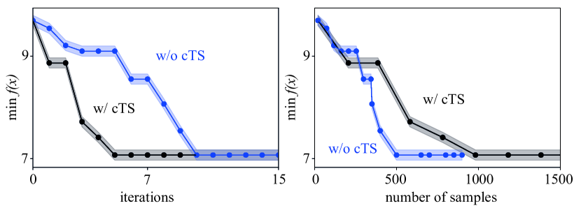
Figure 3: The ablation study of the budgeted batching algorithm with Pest dataset.

Table 5: Budgeted Batching algorithm.

Algorithm 1: Budgeted Batching

Input: feasible region $\pi$, observed dataset $\textbf{D}_{\text{obs}}=(\textbf{X}_{\text{obs}},\textbf{y}_{\text{obs}})$, $\textbf{D}_{\text{ct}}=(\textbf{X}_{\text{ct}},\textbf{y}_{\text{ct}})$,

batch size $n$, surrogate models $f_{\text{obs}},f_{\text{ct}}$

Output: next querying locations $\textbf{X}_{\text{batch}}$

1: $\textbf{X}_{\text{rec}}\sim\pi$

2: $\textbf{w}_{\text{LP}},\textbf{X}_{\text{LP}}\leftarrow\text{cSOBER}(f_{\text{obs}},f_{\text{ct}},\textbf{D}_{\text{obs}},\textbf{D}_{\text{ct}},\textbf{X}_{\text{rec}})$

3: if length($\textbf{X}_{\text{batch}}$) = $n$:

4:     $\textbf{X}_{\text{batch}}=\textbf{X}_{\text{LP}}$

5: else:

6:     $\textbf{X}_{\text{rest}}=\textbf{X}_{\text{rec}}\setminus\textbf{X}_{\text{LP}}$

7:     $\textbf{D}_{\text{obs, hal}}=(\textbf{X}_{\text{LP}},f_{\text{obs}}(\textbf{X}_{\text{LP}})),\quad\textbf{D}_{\text{ct, hal}}=(\textbf{X}_{\text{LP}},f_{\text{ct}}(\textbf{X}_{\text{LP}}))$

8:     $f_{\text{obs, hal}},f_{\text{ct, hal}}\leftarrow\text{HallucinationGPs}(\textbf{D}_{\text{obs}}\cup\textbf{D}_{\text{obs, hal}},\,\textbf{D}_{\text{ct}}\cup\textbf{D}_{\text{ct, hal}})$

9:     $\textbf{X}_{\text{cTS}}\leftarrow\text{cTS}(f_{\text{ob}},f_{\text{ct}},\textbf{X}_{\text{rest}})$

10:     $\textbf{X}_{\text{batch}}=\textbf{X}_{\text{LP}}\cup\textbf{X}_{\text{cTS}}$

11: return $\textbf{X}_{\text{batch}}$

The budgeted batching algorithm flow is explained in Table 5. The algorithm of cTS is SCBO without trust region for generality, which can be found in [20]. Figure 3 explains the difference between algorithms with and without budgeted batching. While the algorithm without cTS (we refer to "w/o cTS") dynamically changes the batch sizes for each iteration depending on the tolerance, the algorithm with cTS (we refer to "w/ cTS") fills the samples until the number of samples reaches the user-defined batch size. "w/ cTS" showed faster convergence than "w/o cTS" from the iteration viewpoint, whereas it is opposite in the figure based on the total number of samples. This indicates that we can use "w/ cTS" for faster convergence for accelerating the optimisation process regardless of the budgets for querying the true functions, and "w/o cTS" for more sample-efficient parallel optimisation in limited budgets. In our experiments, we used "w/ cTS" algorithm throughout the paper for comparison with other algorithms, which can only treat the fixed batch sizes. We emphasise that budgeted sampling with dynamic batch size change is favourable for real-world cases where the budget is limited. The reason why we adopt "w/ cTS" algorithm is for comparison with other baseline algorithms and is not the best use-case for our algorithm cSOBER.

Appendix E algorithm

Table 6: cSOBER algorithm.

Algorithm 2: cSOBER
Input: prior $\pi^{\prime}$, observed dataset $\textbf{D}_{\text{obs}}=(\textbf{X}_{\text{obs}},\textbf{y}_{\text{obs}})$, $\textbf{D}_{\text{ct}}=(\textbf{X}_{\text{ct}},\textbf{y}_{\text{ct}})$
Output: next querying locations $\textbf{X}_{\text{batch}}$
1: $f_{\text{ob}},f_{\text{ct}}\leftarrow\text{InitialiseAndTrainGPs}(\textbf{D}_{\text{ob}},\textbf{D}_{\text{ct}})$
2: $\pi,\rho,\alpha,K_{\text{LP}}\leftarrow\text{FeasibleRegions}(f_{\text{ob}},f_{\text{ct}})$
3: $\textbf{w}_{\text{rec}},\textbf{X}_{\text{rec}},\textbf{X}_{\text{nys}}\sim\text{Sampling}(\pi,\pi^{\prime})$
4: $\epsilon_{\text{rej}}\sim\text{EstimateTolerance}(\rho,\textbf{w}_{\text{rec}},\textbf{X}_{\text{rec}})$
5: $\textbf{w}_{\text{batch}},\textbf{X}_{\text{batch}}\leftarrow\text{LPforBatching}(\textbf{w}_{\text{rec}},\textbf{X}_{\text{rec}},\textbf{X}_{\text{nys}},\alpha,\rho,\epsilon_{\text{rej}},K_{\text{LP}})$
6: return    $\textbf{X}_{\text{batch}}$

E.1 Algorithm flow

The algorithm flow of cSOBER is shown in Table 6. Feasible regions are defined in Section 3.1. Sampling procedure from $\pi$ can be found in the original solving optimisation as Bayesian estimation via recombination (SOBER) paper [2]. Tolerance estimation is in Section 3.1, which is simply the MC estimation of rejection rate $\epsilon_{\text{rej}}:=1-\textbf{w}_{\text{rec}}^{\top}\bigodot_{\ell=1}^{L}\rho_{\ell}(\textbf{X}_{\text{rec}})$. The details for LP part is in Section 3.2.

E.2 Relationship between Constrained Global Optimisation and Quadrature

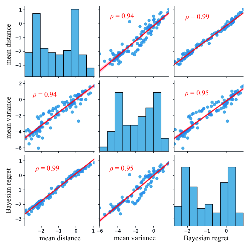
Figure 4: The correlations between Bayesian regret and measure optimisation

To make sure the duality between global optimisation and measure optimisation via quadrature is still preserved under constrainted cases, we empirically compare the $\pi$ shrinkage and Bayesian regret of global optimisation. By following the same procedure in SOBER paper analysis, we obtained the identical results shown in Figure 4. We evaluate the $\pi$ shrinkage and Bayesian regret based on the following definition:

$$\mathbb{E}[\pi(x)] :=\int x\text{d}\pi(x)\approx\textbf{w}_{\text{rec}}^{\top}\textbf{X}_{\text{rec}},$$ (23a)

$$\mathbb{V}\text{ar}[\pi(x)] :=\int|x-\mathbb{E}[\pi(x)]|^{2}\text{d}\pi(x)\approx\textbf{w}_{\text{rec}}^{\top}\text{diag}\Big{[}(\textbf{X}_{\text{rec}}-\mathbb{E}[\pi(x)])^{\top}(\textbf{X}_{\text{rec}}-\mathbb{E}[\pi(x)])\Big{]},$$ (23b)

$$|x^{*}_{\text{true}}-\mathbb{E}[\pi(x)]| \approx\sqrt{\sum_{k=1}^{d}(x^{*}_{\text{true},k}-(\textbf{w}_{\text{rec}}^{\top}\textbf{X}_{\text{rec}})_{k})^{2}},$$ (23c)

BR $$:=|y^{*}_{\text{true}}-\textbf{w}_{\text{batch}}^{\top}f_{\text{true}}(\textbf{X}_{\text{batch}})|.$$ (23d)

we refer to $|x^{*}_{\text{true}}-\mathbb{E}[\pi(x)]|$ as the mean distance, the Euclidean distance between the mean of $\pi$ and the true global maximum $x^{*}_{\text{true}}$, and $\mathbb{V}\text{ar}[\pi(x)]$ as mean variance, corresponding to the $\pi$ shrinkage of which smaller value indicates shrinking. We compared these two metrics against Bayesian regret (BR). Bayesian regret is the batch estimation regret (Theorem 2 in [50]). Experiments were done using cSOBER on the Ackley function (see Table 3) over 10 iterations with 16 repeats of different random seeds (160 data points). Figure 4 shows the linear correlation matrix of these 3 metrics. Both mean distance and variance are highly correlated with Bayesian regret, clearly explaining the $\pi$ shrinkage as the dual objective in Eq. (1) is the good measure of Bayesian regret. In other words, $\pi$ (MC estimate of $x^{*}$) shrinks toward true global maximum $x^{*}_{\text{true}}$ with being smaller variance (more confident), and both linearly correlated to minimising the Bayesian regret.

Appendix F Experimental Details

F.1 Baseline Implementations

We examined our method, cSOBER, with the 8 datasets. All experiments are averaged over 10 repeats with different random seeds. random is the random samples drawn from the prior distribution for each task. As these random samples are aware of categorical or mixed variables, it often outperforms baseline methods that cannot handle them (e.g. cEI in Pest). cEI [56] is the method based on constrained EI AF. We adopted the official implementation on BoTorch [7]. The batching algorithm is based on SAA, a standard in BoTorch. PESC is the method based on constrained PES AF [43]. The official implementaiton in Spearmint is dependent on Python 2 and is no longer supported. Thus, we adopted the implementation on BoTorch [7]. The batching algorithm is based on MC sampling following the original code [41]. However, this code is tremendously slow, which are repeatedly pointed out in BO literature [20]. We set 7 days as the practical limit of execution time allowing for active learning, and PESC exceeds this limit in large batch sizes. We could apply to only Hartmann5 dataset. SCBO is the constrained version of TurBO based on TS and trust region methods. We adopted the official implementation on BoTorch [7] and the same hyperparameters in the original papers [19] for trust region update heuristics. cTS is the constrained TS method. cTS has not been considered in existing work but this is a simple combination of known techniques: we adopt the two-step sampling used in SCBO to TS, as trust region heuristics are not capable to apply to non-Euclidean kernel (e.g. Tanimoto kernel does not have lengthscale hyperparameter). This is coded based on SCBO implementation on BoTorch [7] and just removed the trust region part. PropertyDAG [71] is the method based on qNEHVI AF and [14, 15] for multi-objective optimization. This method assumes (1) ordered constraints but the constraint function is given, (2) multi-objective BO. So it cannot simply apply to our setting as it is. This method is the only one considering ordered case, so we dismantle the components of PropertyDAG to compare in the blackbox ordered constraint case. PropertyDAG consists of three parts: (A) explicit modelling of DAG network in surrogate model [5], (B) zero inflation model to encode ordered constraint information to qNEHVI AF, and (C) resampling of posterior function samples using SAA to be more likely to satisfy the constraint. We cannot apply (A) and (B) for black-box ordered constraint, because (A) is only for white-box ordered constraint (we cannot model of unknown DAG), and (B) is only for multi-objective BO and specific AF. Thus, we extracted the last part, (C) resampling with SAA, and combined this with cEI, which we refer to PropertyDAG in this paper. We can say this as just resampled version of cEI. The implementation is based on cEI implementation on BoTorch [7] and added the resampling part.

cEI, PESC, SCBO, PropertyDAG are not compatible to categorical and mixed input spaces due to the continuity assumption in these methods. To enable comparison against these methods, we adopt thresholding in discrete or mixed problems: namely, we optimise the discrete variables as bounded continuous variables, then the selected continuous locations are classified into the closest original discrete values. For the graph space, we deem the search space itself to be a graph and the objective is to find a subgraph. This is different from, for example, the drug discovery problem, whose input variables are graphs but the space itself is non-Euclidean discrete set of drugs. In contrast, the graph space is over the large graph, and the graph example is only one. Thus, cTS is the only method applicable to graph space other than cSOBER. Our code is built upon PyTorch-based libraries [72, 22, 7, 31] and Gurobipy [33] is used to solve LP. All baseline methods are official implementations in BoTorch or coded with BoTorch [7].

F.2 Dataset

Ackely

Ackley funciton is defined as:

$$f(x):=-a\exp\left[-b\sqrt{\frac{1}{d}\sum_{i=1}^{d}x_{i}^{2}}\right]-\exp\left[\frac{1}{d}\sum_{i=1}^{d}\cos(cx_{i})\right]+a+\exp(1)$$ (24)

where $a=20,c=2\pi,d=23$. We take the negative Ackley function as the objective of BO to make this optimisation problem maximisation. We modified the original Ackley function into a 23-dimensional function with the mixed spaces of 3 continuous and 20 binary inputs from $[0,1]^{20}$, following [2]. The batch size $n$ is 200. The continuous prior is the uniform distribution ranging from [-1, 1]. The binary prior is the Bernoulli distribution with unbiased weights 0.5. We assume each of continuous and binary priors at each dimension are independent. We added the two constraints; (1) $x_{1}\geq 0$ and (2) $x_{2}\geq 0$, where $x_{1}$ and $x_{2}$ are the first and second dimension of continuous inputs. We assume both constraints are blackbox, coupled, unordered, deterministic, continuous, and cheap.

Hartmann

Hartmann 6-dimensional function is defined as:

$$f(x) :=-\sum_{i=1}^{4}\alpha_{i}\exp\left(-\sum_{j=1}^{6}A_{ij}(x_{j}-P_{ij})^{2}\right),$$ (25)

$$\alpha =(1.0,1.2,3.0,3.2)^{\top},$$ (26)

A $$=\begin{pmatrix}10&3&17&3.5&1.7&8\\ 0.05&10&17&0.1&8&14\\ 3&3.5&1.7&10&17&8\\ 17&8&0.05&10&0.1&14\\ \end{pmatrix},$$ (27)

P $$=\begin{pmatrix}1312&1696&5569&124&8283&5886\\ 2329&4135&8307&3736&1004&9991\\ 2348&1451&3522&2883&3047&6650\\ 4047&8828&8732&5743&1091&381\\ \end{pmatrix}$$ (28)

We take the negative Hartmann function as the objective of BO to make this optimisation problem maximisation. All input variables are continuous with bounds $[0,1]^{6}$. The batch size $n$ is 100. The continuous prior is the uniform distribution ranging from [0, 1], following [2]. We added two constraints; (1) $\sum_{i=1}^{d}x_{d}\geq 0.15$ and (2) $\sum_{i=1}^{d}x_{d}\leq 3$. We assume these two constraints are blackbox, coupled, unordered, deterministic, continuous, and cheap. We compared the same problem with different batch sizes 5 and 100, where we refer to Hartman5 and Hartmann100, respectively.

PestControl

Pest Control (PestControl in the main) is proposed in [68], which is a multi-categorical optimisation problem (15 dimensions, 5 categories for each dimension). We wish to optimise the effectiveness of pesticide by choosing the 5 actions (selection of pesticides from 4 different firms, or not using any of it), but penalised by their prices. This choice is a sequential decision of 15 stages, and the objective function is expressed as the cumulative loss function with the total of both cost and the portion having pest. The batch size $n$ is 200. We set the categorical prior with equal weights for each choice (discrete uniform distribution). Code is used in https://github.com/xingchenwan/Casmopolitan [89].

We added 2 constraints for a more realistic situation. The first constraint is ecosystem change, which assumes exterminating pests too much causes other harmful pests/animals to increase when reach the hidden threshold. The portion of the product having pest follows the dynamics below:

$$z_{i} =\alpha_{i}(1-x_{i})(1-z_{i-1})+(1-\Gamma_{i}x_{i})z_{i-1},$$ (29)

$$z_{i} \geq z_{\text{limit}},$$ (30)

where $i$ is the number of pest control cycle (15 in total), $z$ is the portion of the product having pest, $x$ is the effectiveness of pesticide that follows beta distribution with the parameters, which has been adjusted according to the sequence of actions taken in previous control points, $\alpha$ is the action taken (selection of pesticides from 4 different firms, or not using any of it), and $z_{\text{limit}}$ is the threshold for ecosystem change (we set $1e-3$). Eq. 30 is the constraint of echosystem change, and we assume the latent variable $z_{i}$ is observable. We assume this constraint is blackbox, coupled, unordered, deterministic, continuous, and expensive.

The second constraint is neighbour disputes, which assume some of the pesticides have unfavourable smell. Neighbours objection follows Bernoulli distribution and its weights based on the proportion of certain pesticide types and random Gaussian noise. Thus, the feedback to this constraint is in the noisy binary value. If the neighbours’ objection is larger than supportive opinion $\theta_{\text{pest}}>0.5$, a decision maker stops spraying pesticides, thus, objective value cannot be evaluated. We assume this constraint is blackbox, coupled, ordered, probabilistic, binary, and expensive.

Malaria

The objective is to discover an anti-Malarial drug exhibiting the smallest EC50 value, which is defined as the concentration of the drug which gives half the maximal response. The lower the concentration, the more effective (better) the drug. The dataset consists of 20,746 small molecules taken from the P. falciparum whole cell screening derived by the Novatis-GNF Malaria Box [83]. The molecules are represented as SMILES string, and are converted into 2048-dimensional binary features for Tanimoto kernel. We set four safety constraints, all of which are rule of thumb for judging molecules likely to be oral drugs, shared in drug discovery community ([57], [87], [10], [62]).

The first is the Lipinski’s rule of five [57], (A) no more than 5 hydrogen bond donors, (B) no more than 10 hydrogen bond acceptors, (C) A molecular mass less than 500 daltons, (D) A calculated octanol-water partition coefficient that does not exceed 5, (E) no more than 5 roratable bonds. The second is the Veber filter [87], (A) no more than 10 rotatable bonds, (B) a polar surface area that does not exceed 140. The third is the REOS filter [10], (A) A molecular mass more than 200 daltons and less than 500 daltons, (B) A calculated octanol-water partition coefficient that exceeds -5 but does not exceed 5, (C) no more than 5 hydrogen bond donors, (D) no more than 10 hydrogen bond acceptors, (E) no more than 8 roratable bonds, (F) more than 15 but less than 50 heavy atoms, (G) more than -2 but less than 2 formal charge. The fourth is the drug likeliness filter, (A) A molecular mass less than 400 daltons, (B) at least one ring structure, (C) no more than 5 roratable bonds, (D) no more than 5 hydrogen bond donors, (E) no more than 10 hydrogen bond acceptors, (F) A calculated octanol-water partition coefficient that does not exceed 5. We assume all of the above four constraints are coupled, ordered, probabilistic, continuous, and expensive.

Solvent

The objective is to discover a better solvent for lithium-ion batteries having larger dipole moments, which is the key descriptor for the solvation of lithium-ions in electrolytes, increasing the ratio of electro-mobile Li-ions. The higher the dipole moment becomes, the larger (better) the ionic conductivity does. The dataset with 133,055 small molecules predicted by the quantum-chemical computations using density functional theory, known as QM9 dataset [75]. We set 3 constraints on temperature performances, flash point, melting point, and boiling points, corresponding to flammability, low-temperature performance, and high-temperature performance, respectively. These values are estimated using molecule descriptors using Mordred library [64], and correlation taken from [13]. We assume these constraints can be queried by different experiments, and is easier than dipole moment measurements. We assume these constraints are decoupled, ordered, probabilistic, continuous, and expensive.

FindFixer

This task is to find the fixer connecting influencers rather than finding the most popular influencer on the social networks graph. A job seeker who wishes to be a celebrity explores the fixer to ask introductions based on graph data using the centrality analysis. Finding a node needs to search on a website or meet in person, both of which are expensive to evaluate. Fixer can be interpreted as a node with maximum eigenvector centrality under constraints on the degree centrality that does not exceed the threshold [53]. In other words, finding the node that is connected to the largest number of nodes with many edges but is not having many edges itself. A job seeker wishes to find the fixer who connects influencers with similar popularity (degree centrality). Thus, the node is constrained based on the degree centrality, and other hidden preference factors. A job seeker judges constraints as a binary value, and the judgment is possibly shaky. We assume this constraint is blackbox, coupled, ordered, probabilistic, mixture of binary/continuous, and mixture of cheap/expensive. We assume the domain is defined as a social network graph synthesized by the Barábsi–Albert model (BA) [9].

TeamOpt

This task is to organise a team consisting of the most diverse skill sets of members [90]. The objective is measured by the entropy of the skills of members, assuming the optimal team is when each member is specialised in one skill, and the whole skill distribution is close to uniform. Such teams are positioned on the node of the supergraph, of which edge is the similarity between teams defined as the Jaccord index. The constraints are interpersonal relationships. Every combination of two individuals from $N$ candidates has unobservable hidden continuous likability from 0 to 1. The first is the mean likability constraint, which is the mean of likeability between all possible combinations of members that should be larger than equal-chance. The second is the tragedy-avoidance constraint, which is a binary judge that none of them has a likability lower than a threshold. The third is a flat-relationship constraint, which assumes an entropy of likability must be higher than a threshold. As likability is unobservable, a decision-maker needs to seek advice for many colleagues who partially know each constraint but are noisy estimations. We assume all three constraints are decoupled, ordered, probabilistic, binary, and expensive.

F.3 Experimental results

Table 7: Experimental results on best objective function value (see Table 3 ) obtained after 15 iterations. Reported is average $\pm$ 1 standard error over 10 repeated runs. Most experiments were conducted on large batch sizes of over 100. N.Ecld. is short for non-Euclidean space.

baselines	Ackley	Hart- mann100	Hart- mann5	Pest Control	Malaria	Solvent	Find Fixer	Team Opt
Random	0.272 ± 0.01	-0.108 ± 0.03	-0.039 ± 0.05	8.582 ± 0.04	-2.381 ± 0.10	-1.015 ± 0.04	-0.908 ± 0.09	-1.647 ± 0.01
cEI	-0.002 ± 0.02	-0.218 ± 0.04	-0.065 ± 0.06	8.737 ± 0.07	Combinatorial explosion in N.Ecld.
cTS	0.234 ± 0.01	-0.577 ± 0.03	-0.550 ± 0.06	8.513 ± 0.01	-2.414 ± 0.08	1.179 ± 0.03	-0.742 ± 0.16	-0.586 ± 0.11
PESC	too slow (>7 days)		-0.090 ± 0.06	too slow	N.Ecld. and too slow (>7 days)
SCBO	0.255 ± 0.01	-0.842 ± 0.01	-1.227 ± 0.18	7.484 ± 0.13	No lengthscale in kernel for trust region and in N.Ecld.
Property DAG	-0.041 ± 0.03	-0.125 ± 0.05	-0.092 ± 0.06	8.811 ± 0.06	Combinatorial explosion in N.Ecld.
cSOBER	-3.588 ± 0.04	-1.303 ± 0.04	-1.276 ± 0.08	7.070 ± 0.00	-2.466 ± 0.08	1.199 ± 0.00	-0.195 ± 0.00	-1.895 ± 0.01

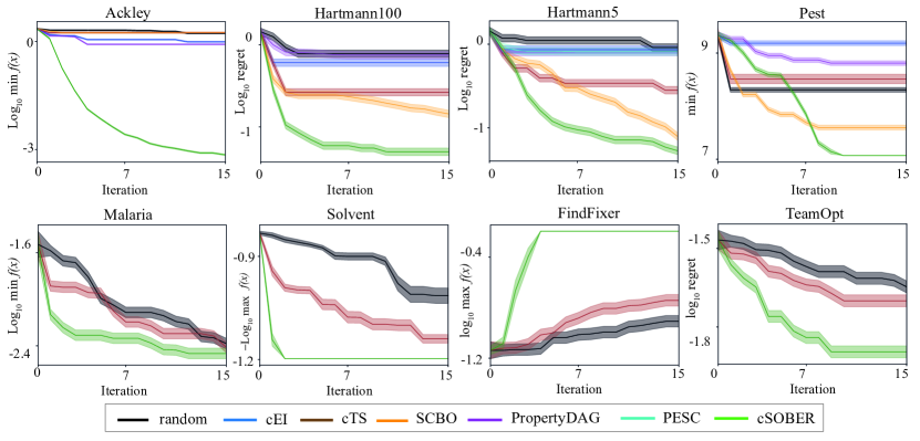
Figure 5: We evaluate cSOBER across 2 synthetic functions and 5 real-world drug discovery datasets. Top: Log regret or log best observations, Bottom: Log overhead in seconds as a function of iterations. Lines and shaded area denote mean $\pm$ 1 standard error. The batch size is 100 or 200 (see Table 3).

The experimental results are shown in Table 7 for the values at 15th iterations, and Figure 5 for the learning curve over iterations. We find the some mistakes in values in Table 4 after main paper submission, so the Table 7 is the corrected result. The mistakes can be found comparing between Tables 4 and 7, but the corrected part is only on both Hartman datasets, on random, cEI, PropertyDAG. The main result is not changed (cSOBER was the most performant throughout the experiments).

References

- [1] Masaki Adachi. High-dimensional discrete Bayesian optimization with self-supervised representation learning for data-efficient materials exploration. In NeurIPS 2021 AI for Science Workshop, 2021.
- [2] Masaki Adachi, Satoshi Hayakawa, Saad Hamid, Martin Jørgensen, Harald Oberhauser, and Micheal A Osborne. SOBER: Scalable batch Bayesian optimization and quadrature using recombination constraints. arXiv preprint arXiv:2301.11832, 2023.
- [3] Masaki Adachi, Satoshi Hayakawa, Martin Jørgensen, Harald Oberhauser, and Michael A Osborne. Fast Bayesian inference with batch Bayesian quadrature via kernel recombination. In Advances in Neural Information Processing Systems, volume 35, 2022. URL: https://proceedings.neurips.cc/paper_files/paper/2022/file/697200c9d1710c2799720b660abd11bb-Paper-Conference.pdf.
- [4] Masaki Adachi, Yannick Kuhn, Birger Horstmann, Michael A Osborne, and David A Howey. Bayesian model selection of lithium-ion battery models via bayesian quadrature. arXiv preprint arXiv:2210.17299, 2022.
- [5] Raul Astudillo and Peter Frazier. Bayesian optimization of function networks. Advances in neural information processing systems, 34:14463–14475, 2021.
- [6] Javad Azimi, Alan Fern, and Xiaoli Fern. Batch Bayesian optimization via simulation matching. Advances in Neural Information Processing Systems, 23, 2010.
- [7] Maximilian Balandat, Brian Karrer, Daniel Jiang, Samuel Daulton, Ben Letham, Andrew G Wilson, and Eytan Bakshy. BoTorch: a framework for efficient Monte-Carlo Bayesian optimization. Advances in neural information processing systems, 33:21524–21538, 2020.
- [8] Ricardo Baptista and Matthias Poloczek. Bayesian optimization of combinatorial structures. In Jennifer Dy and Andreas Krause, editors, Proceedings of the 35th International Conference on Machine Learning, volume 80 of Proceedings of Machine Learning Research, pages 462–471. PMLR, 10–15 Jul 2018. URL: https://proceedings.mlr.press/v80/baptista18a.html.
- [9] Albert-László Barabási and Réka Albert. Emergence of scaling in random networks. science, 286(5439):509–512, 1999.
- [10] Mark S Butler. The role of natural product chemistry in drug discovery. Journal of natural products, 67(12):2141–2153, 2004.
- [11] Arnaud Carpentier, Ila Nimgaonkar, Virginia Chu, Yuchen Xia, Zongyi Hu, and T Jake Liang. Hepatic differentiation of human pluripotent stem cells in miniaturized format suitable for high-throughput screen. Stem Cell Research, 16(3):640–650, 2016.
- [12] Henry R Chai and Roman Garnett. Improving quadrature for constrained integrands. In The 22nd International Conference on Artificial Intelligence and Statistics, pages 2751–2759. PMLR, 2019.
- [13] Ana E Comesana, Tyler T Huntington, Corinne D Scown, Kyle E Niemeyer, and Vi H Rapp. A systematic method for selecting molecular descriptors as features when training models for predicting physiochemical properties. Fuel, 321:123836, 2022.
- [14] Samuel Daulton, Maximilian Balandat, and Eytan Bakshy. Differentiable expected hypervolume improvement for parallel multi-objective bayesian optimization. Advances in Neural Information Processing Systems, 33:9851–9864, 2020.
- [15] Samuel Daulton, Maximilian Balandat, and Eytan Bakshy. Parallel bayesian optimization of multiple noisy objectives with expected hypervolume improvement. Advances in Neural Information Processing Systems, 34:2187–2200, 2021.
- [16] Samuel Daulton, Xingchen Wan, David Eriksson, Maximilian Balandat, Michael A Osborne, and Eytan Bakshy. Bayesian optimization over discrete and mixed spaces via probabilistic reparameterization. arXiv preprint arXiv:2210.10199, 2022.
- [17] Aryan Deshwal, Syrine Belakaria, and Janardhan Rao Doppa. Mercer features for efficient combinatorial bayesian optimization. Proceedings of the AAAI Conference on Artificial Intelligence, 35(8):7210–7218, 2021. URL: https://ojs.aaai.org/index.php/AAAI/article/view/16886, doi:10.1609/aaai.v35i8.16886.
- [18] Petros Drineas and Michael W. Mahoney. On the nystrom method for approximating a gram matrix for improved kernel-based learning. Journal of Machine Learning Research, 6(72):2153–2175, 2005. URL: http://jmlr.org/papers/v6/drineas05a.html.
- [19] David Eriksson, Michael Pearce, Jacob Gardner, Ryan D Turner, and Matthias Poloczek. Scalable global optimization via local Bayesian optimization. Advances in neural information processing systems, 32, 2019.
- [20] David Eriksson and Matthias Poloczek. Scalable constrained Bayesian optimization. In International Conference on Artificial Intelligence and Statistics, pages 730–738. PMLR, 2021.
- [21] Matthias Feurer, Aaron Klein, Katharina Eggensperger, Jost Springenberg, Manuel Blum, and Frank Hutter. Efficient and robust automated machine learning. Advances in neural information processing systems, 28, 2015.
- [22] Jacob Gardner, Geoff Pleiss, Kilian Q Weinberger, David Bindel, and Andrew G Wilson. GPyTorch: Blackbox matrix-matrix Gaussian process inference with GPU acceleration. Advances in neural information processing systems, 31, 2018.
- [23] Jacob R Gardner, Matt J Kusner, Zhixiang Eddie Xu, Kilian Q Weinberger, and John P Cunningham. Bayesian optimization with inequality constraints. In ICML, volume 2014, pages 937–945, 2014.
- [24] Roman Garnett. Bayesian optimization. Cambridge University Press, 2023.
- [25] Michael A Gelbart, Jasper Snoek, and Ryan P Adams. Bayesian optimization with unknown constraints. In 30th Conference on Uncertainty in Artificial Intelligence, UAI, volume 2014, pages 250––259, 2014.
- [26] Rafael Gómez-Bombarelli, Jennifer N Wei, David Duvenaud, José Miguel Hernández-Lobato, Benjamín Sánchez-Lengeling, Dennis Sheberla, Jorge Aguilera-Iparraguirre, Timothy D Hirzel, Ryan P Adams, and Alán Aspuru-Guzik. Automatic chemical design using a data-driven continuous representation of molecules. ACS central science, 4(2):268–276, 2018.
- [27] Javier González, Zhenwen Dai, Philipp Hennig, and Neil Lawrence. Batch Bayesian optimization via local penalization. In Artificial intelligence and statistics, pages 648–657. PMLR, 2016.
- [28] Javier González, Michael Osborne, and Neil Lawrence. Glasses: Relieving the myopia of bayesian optimisation. In Artificial Intelligence and Statistics, pages 790–799. PMLR, 2016.
- [29] Robert B Gramacy, Genetha A Gray, Sébastien Le Digabel, Herbert KH Lee, Pritam Ranjan, Garth Wells, and Stefan M Wild. Modeling an augmented lagrangian for blackbox constrained optimization. Technometrics, 58(1):1–11, 2016.
- [30] Ryan-Rhys Griffiths and José Miguel Hernández-Lobato. Constrained Bayesian optimization for automatic chemical design using variational autoencoders. Chemical science, 11(2):577–586, 2020.
- [31] Ryan-Rhys Griffiths, Leo Klarner, Henry Moss, Aditya Ravuri, Sang T Truong, Bojana Rankovic, Yuanqi Du, Arian Rokkum Jamasb, Julius Schwartz, Austin Tripp, et al. GAUCHE: A library for Gaussian processes in chemistry. In ICML 2022 2nd AI for Science Workshop, 2022.
- [32] Tom Gunter, Michael A Osborne, Roman Garnett, Philipp Hennig, and Stephen J Roberts. Sampling for inference in probabilistic models with fast Bayesian quadrature. Advances in neural information processing systems, 27, 2014.
- [33] Gurobi Optimization, LLC. Gurobi Optimizer Reference Manual, 2022. URL: https://www.gurobi.com.
- [34] Michael U Gutmann and Jukka Corander. Bayesian optimization for likelihood-free inference of simulator-based statistical models. Journal of Machine Learning Research, 2016.
- [35] Satoshi Hayakawa, Terry Lyons, and Harald Oberhauser. Estimating the probability that a given vector is in the convex hull of a random sample. Probability Theory and Related Fields, 185:705–746, 2023.
- [36] Satoshi Hayakawa, Harald Oberhauser, and Terry Lyons. Positively weighted kernel quadrature via subsampling. In S. Koyejo, S. Mohamed, A. Agarwal, D. Belgrave, K. Cho, and A. Oh, editors, Advances in Neural Information Processing Systems, volume 35, pages 6886–6900. Curran Associates, Inc., 2022. URL: https://proceedings.neurips.cc/paper_files/paper/2022/file/2dae7d1ccf1edf76f8ce7c282bdf4730-Paper-Conference.pdf.
- [37] Satoshi Hayakawa, Harald Oberhauser, and Terry Lyons. Hypercontractivity meets random convex hulls: analysis of randomized multivariate cubatures. Proceedings of the Royal Society A, 479(2273):20220725, 2023. URL: https://royalsocietypublishing.org/doi/abs/10.1098/rspa.2022.0725, doi:10.1098/rspa.2022.0725.
- [38] Satoshi Hayakawa, Harald Oberhauser, and Terry Lyons. Sampling-based Nyström approximation and kernel quadrature. arXiv preprint arXiv:2301.09517, 2023.
- [39] Philipp Hennig, Michael A Osborne, and Hans P Kersting. Probabilistic Numerics: Computation as Machine Learning. Cambridge University Press, 2022.
- [40] Philipp Hennig and Christian J Schuler. Entropy search for information-efficient global optimization. Journal of Machine Learning Research, 13(6), 2012.
- [41] José Miguel Hernández-Lobato, Michael Gelbart, Matthew Hoffman, Ryan Adams, and Zoubin Ghahramani. Predictive entropy search for Bayesian optimization with unknown constraints. In International conference on machine learning, pages 1699–1707. PMLR, 2015.
- [42] José Miguel Hernández-Lobato, Michael A. Gelbart, Ryan P. Adams, Matthew W. Hoffman, and Zoubin Ghahramani. A general framework for constrained Bayesian optimization using information-based search. Journal of Machine Learning Research, 17(1):5549–5601, 2016.
- [43] José Miguel Hernández-Lobato, Matthew W Hoffman, and Zoubin Ghahramani. Predictive entropy search for efficient global optimization of black-box functions. Advances in neural information processing systems, 27, 2014.
- [44] José Miguel Hernández-Lobato, James Requeima, Edward O Pyzer-Knapp, and Alán Aspuru-Guzik. Parallel and distributed Thompson sampling for large-scale accelerated exploration of chemical space. In International conference on machine learning, pages 1470–1479. PMLR, 2017.
- [45] Neil Houlsby, Ferenc Huszár, Zoubin Ghahramani, and Máté Lengyel. Bayesian active learning for classification and preference learning. arXiv preprint arXiv:1112.5745, 2011.
- [46] Ferenc Huszár and David Duvenaud. Optimally-weighted herding is bayesian quadrature. In Proceedings of the Twenty-Eighth Conference on Uncertainty in Artificial Intelligence, UAI’12, page 377–386, Arlington, Virginia, USA, 2012. AUAI Press.
- [47] Carl Hvarfner, Frank Hutter, and Luigi Nardi. Joint entropy search for maximally-informed Bayesian optimization. arXiv preprint arXiv:2206.04771, 2022.
- [48] Donald R Jones, Matthias Schonlau, and William J Welch. Efficient global optimization of expensive black-box functions. Journal of Global optimization, 13(4):455–492, 1998.
- [49] Hiroshi Kajino. Molecular hypergraph grammar with its application to molecular optimization. In International Conference on Machine Learning, pages 3183–3191. PMLR, 2019.
- [50] Kirthevasan Kandasamy, Akshay Krishnamurthy, Jeff Schneider, and Barnabás Póczos. Parallelised Bayesian optimisation via Thompson sampling. In International Conference on Artificial Intelligence and Statistics, pages 133–142. PMLR, 2018.
- [51] Tarun Kathuria, Amit Deshpande, and Pushmeet Kohli. Batched Gaussian process bandit optimization via determinantal point processes. Advances in Neural Information Processing Systems, 29, 2016.
- [52] Diederik P Kingma and Max Welling. Auto-encoding variational bayes. arXiv preprint arXiv:1312.6114, 2013.
- [53] Christine Kiss and Martin Bichler. Identification of influencers—measuring influence in customer networks. Decision Support Systems, 46(1):233–253, 2008.
- [54] Sanjiv Kumar, Mehryar Mohri, and Ameet Talwalkar. Sampling methods for the nyström method. The Journal of Machine Learning Research, 13(1):981–1006, 2012.
- [55] Harold J Kushner. A new method of locating the maximum point of an arbitrary multipeak curve in the presence of noise. Journal of basic engineering, 86:97 – 106, 1964.
- [56] Benjamin Letham, Brian Karrer, Guilherme Ottoni, and Eytan Bakshy. Constrained Bayesian optimization with noisy experiments. Bayesian Analysis, 14(2):495 – 519, 2019. doi:10.1214/18-BA1110.
- [57] Christopher A Lipinski, Franco Lombardo, Beryl W Dominy, and Paul J Feeney. Experimental and computational approaches to estimate solubility and permeability in drug discovery and development settings. Advanced drug delivery reviews, 23(1-3):3–25, 1997.
- [58] C. Litterer and T. Lyons. High order recombination and an application to cubature on Wiener space. The Annals of Applied Probability, 22(4):1301–1327, 2012.
- [59] Xianggen Liu, Qiang Liu, Sen Song, and Jian Peng. A chance-constrained generative framework for sequence optimization. In International Conference on Machine Learning, pages 6271–6281. PMLR, 2020.
- [60] Alaa Maalouf, Ibrahim Jubran, and Dan Feldman. Fast and accurate least-mean-squares solvers. Advances in Neural Information Processing Systems, 32, 2019.
- [61] Natalie Maus, Haydn Jones, Juston Moore, Matt J Kusner, John Bradshaw, and Jacob Gardner. Local latent space bayesian optimization over structured inputs. Advances in Neural Information Processing Systems, 35:34505–34518, 2022.
- [62] Masahiro Mochizuki, Shogo D Suzuki, Keisuke Yanagisawa, Masahito Ohue, and Yutaka Akiyama. Qex: target-specific druglikeness filter enhances ligand-based virtual screening. Molecular Diversity, 23:11–18, 2019.
- [63] Jonas Močkus. On bayesian methods for seeking the extremum. In Optimization Techniques IFIP Technical Conference: Novosibirsk, July 1–7, 1974, pages 400–404. Springer, 1975.
- [64] Hirotomo Moriwaki, Yu-Shi Tian, Norihito Kawashita, and Tatsuya Takagi. Mordred: a molecular descriptor calculator. Journal of cheminformatics, 10(1):1–14, 2018.
- [65] Henry B Moss, David S Leslie, Javier Gonzalez, and Paul Rayson. Gibbon: General-purpose information-based bayesian optimisation. The Journal of Machine Learning Research, 22(1):10616–10664, 2021.
- [66] Vu Nguyen, Santu Rana, Sunil K Gupta, Cheng Li, and Svetha Venkatesh. Budgeted batch bayesian optimization. In 2016 IEEE 16th International Conference on Data Mining (ICDM), pages 1107–1112. IEEE, 2016.
- [67] Pascal Notin, José Miguel Hernández-Lobato, and Yarin Gal. Improving black-box optimization in vae latent space using decoder uncertainty. Advances in Neural Information Processing Systems, 34:802–814, 2021.
- [68] Changyong Oh, Jakub Tomczak, Efstratios Gavves, and Max Welling. Combinatorial Bayesian optimization using the graph Cartesian product. Advances in Neural Information Processing Systems, 32, 2019.
- [69] Anthony O’Hagan. Bayes–hermite quadrature. Journal of statistical planning and inference, 29(3):245–260, 1991.
- [70] Michael Osborne, Roman Garnett, Zoubin Ghahramani, David K Duvenaud, Stephen J Roberts, and Carl Rasmussen. Active learning of model evidence using Bayesian quadrature. Advances in neural information processing systems, 25, 2012.
- [71] Ji Won Park, Samuel Stanton, Saeed Saremi, Andrew Watkins, Henri Dwyer, Vladimir Gligorijevic, Richard Bonneau, Stephen Ra, and Kyunghyun Cho. Propertydag: Multi-objective bayesian optimization of partially ordered, mixed-variable properties for biological sequence design. arXiv preprint arXiv:2210.04096, 2022.
- [72] Adam Paszke, Sam Gross, Francisco Massa, Adam Lerer, James Bradbury, Gregory Chanan, Trevor Killeen, Zeming Lin, Natalia Gimelshein, Luca Antiga, et al. PyTorch: An imperative style, high-performance deep learning library. Advances in neural information processing systems, 32, 2019.
- [73] Victor Picheny, Robert B Gramacy, Stefan Wild, and Sebastien Le Digabel. Bayesian optimization under mixed constraints with a slack-variable augmented lagrangian. Advances in neural information processing systems, 29, 2016.
- [74] Liva Ralaivola, Sanjay J Swamidass, Hiroto Saigo, and Pierre Baldi. Graph kernels for chemical informatics. Neural networks, 18(8):1093–1110, 2005.
- [75] Raghunathan Ramakrishnan, Pavlo O Dral, Matthias Rupp, and O Anatole Von Lilienfeld. Quantum chemistry structures and properties of 134 kilo molecules. Scientific data, 1(1):1–7, 2014.
- [76] Carl Edward Rasmussen, Christopher KI Williams, et al. Gaussian processes for machine learning, volume 1. Springer, 2006.
- [77] Danilo Jimenez Rezende, Shakir Mohamed, and Daan Wierstra. Stochastic backpropagation and approximate inference in deep generative models. In International conference on machine learning, pages 1278–1286. PMLR, 2014.
- [78] Christoffer Riis, Francisco N Antunes, Frederik Boe Hüttel, Carlos Lima Azevedo, and Francisco Camara Pereira. Bayesian active learning with fully Bayesian Gaussian processes. arXiv preprint arXiv:2205.10186, 2022.
- [79] Binxin Ru, Ahsan Alvi, Vu Nguyen, Michael A Osborne, and Stephen Roberts. Bayesian optimisation over multiple continuous and categorical inputs. In International Conference on Machine Learning, pages 8276–8285. PMLR, 2020.
- [80] Matthias Schonlau, William J Welch, and Donald R Jones. Global versus local search in constrained optimization of computer models. Lecture notes-monograph series, pages 11–25, 1998.
- [81] H Sebastian Seung, Manfred Opper, and Haim Sompolinsky. Query by committee. In Proceedings of the fifth annual workshop on Computational learning theory, pages 287–294, 1992.
- [82] Edward Snelson, Zoubin Ghahramani, and Carl Rasmussen. Warped Gaussian processes. Advances in neural information processing systems, 16, 2003.
- [83] Thomas Spangenberg, Jeremy N Burrows, Paul Kowalczyk, Simon McDonald, Timothy NC Wells, and Paul Willis. The open access malaria box: a drug discovery catalyst for neglected diseases. PloS one, 8(6):e62906, 2013.
- [84] Niranjan Srinivas, Andreas Krause, Sham M Kakade, and Matthias Seeger. Gaussian process optimization in the bandit setting: No regret and experimental design. arXiv preprint arXiv:0912.3995, 2009.
- [85] M. Tchernychova. Carathéodory cubature measures. PhD thesis, University of Oxford, 2015.
- [86] Alexander Thebelt, Calvin Tsay, Robert Lee, Nathan Sudermann-Merx, David Walz, Behrang Shafei, and Ruth Misener. Tree ensemble kernels for bayesian optimization with known constraints over mixed-feature spaces. Advances in Neural Information Processing Systems, 35:37401–37415, 2022.
- [87] Daniel F Veber, Stephen R Johnson, Hung-Yuan Cheng, Brian R Smith, Keith W Ward, and Kenneth D Kopple. Molecular properties that influence the oral bioavailability of drug candidates. Journal of medicinal chemistry, 45(12):2615–2623, 2002.
- [88] Julien Villemonteix, Emmanuel Vazquez, and Eric Walter. An informational approach to the global optimization of expensive-to-evaluate functions. Journal of Global Optimization, 44(4):509–534, 2009.
- [89] Xingchen Wan, Vu Nguyen, Huong Ha, Binxin Ru, Cong Lu, and Michael A Osborne. Think global and act local: Bayesian optimisation over high-dimensional categorical and mixed search spaces. arXiv preprint arXiv:2102.07188, 2021.
- [90] Xingchen Wan, Pierre Osselin, Henry Kenlay, Binxin Ru, Michael A. Osborne, and Xiaowen Dong. Bayesian optimisation of functions on graphs. arXiv preprint arXiv:2306.05304, 2023.
- [91] Zi Wang and Stefanie Jegelka. Max-value entropy search for efficient Bayesian optimization. In International Conference on Machine Learning, pages 3627–3635. PMLR, 2017.
- [92] Florian Wenzel, Théo Galy-Fajou, Christan Donner, Marius Kloft, and Manfred Opper. Efficient gaussian process classification using pòlya-gamma data augmentation. In Proceedings of the AAAI Conference on Artificial Intelligence, pages 5417–5424, 2019.
- [93] Jian Wu, Saul Toscano-Palmerin, Peter I Frazier, and Andrew Gordon Wilson. Practical multi-fidelity Bayesian optimization for hyperparameter tuning. In Uncertainty in Artificial Intelligence, pages 788–798. PMLR, 2020.
- [94] Yin-Cong Zhi, Yin Cheng Ng, and Xiaowen Dong. Gaussian processes on graphs via spectral kernel learning. IEEE Transactions on Signal and Information Processing over Networks, 2023.