Newton-based alternating methods for the ground state of a class of multi-component Bose-Einstein condensates

Abstract

The computation of the ground states of special multi-component Bose-Einstein condensates (BECs) can be formulated as an energy functional minimization problem with spherical constraints. It leads to a nonconvex quartic-quadratic optimization problem after suitable discretizations. First, we generalize the Newton-based methods for single-component BECs to the alternating minimization scheme for multi-component BECs. Second, the global convergent alternating Newton-Noda iteration (ANNI) is proposed. In particular, we prove the positivity preserving property of ANNI under mild conditions. Finally, our analysis is applied to a class of more general ”multi-block” optimization problems with spherical constraints. Numerical experiments are performed to evaluate the performance of proposed methods for different multi-component BECs, including pseudo spin-1/2, anti-ferromagnetic spin-1 and spin-2 BECs. These results support our theory and demonstrate the efficiency of our algorithms.

Key words. Newton method, alternating method, ground state, multi-component Bose-Einstein condensates

Mathematics Subject Classification. 49M15, 90C26, 35Q55, 65N25

1 Introduction

Since the first realization of Bose-Einstein condensates (BECs) was announced in 1995 [1, 2, 3], numerous researchers have been attracted into the theoretical studies and numerical methods for the single-component BEC [4, 5, 6, 7, 8, 9]. While the pioneering experiments were conducted for single species of atoms, it is a natural generalization to explore the multi-component BEC system. Through optical confinements, various spinor condensates have been achieved and revealed exciting phenomena absent in single-component BECs, including pseudo spin-1/2, spin-1 and spin-2 condensates [10, 11, 12, 13]. In this growing research direction, mathematical models and numerical simulation have been playing an important role in understanding the theoretical part of spinor BECs [14, 15].

One of the fundamental problems in BECs is to find the ground state, which is defined as the minimizer of the Gross-Pitaevskii (GP) energy functional minimization problem subject to some physical constraints [16, 17]. The simplest multi-component BEC is the binary mixture. Furthermore, it has been proved that the energy functional minimization problem for spin-$F~{}(F=1,2)$ BEC can be reduced to a two-component BEC problem under some conditions [18, 16]. Computing the ground state of such a two-component BEC can be expressed as

$$\min{} E(\Phi)=\int_{\mathbb{R}^{d}}\left[\frac{1}{2}(|\nabla\phi_{1}|^{2}+|\nabla\phi_{2}|^{2})+V(\mathbf{x})(|\phi_{1}|^{2}+|\phi_{2}|^{2})\right.$$ (1)

$$\left.+\frac{1}{2}\beta_{11}|\phi_{1}|^{4}+\frac{1}{2}\beta_{22}|\phi_{2}|^{4}+\beta_{12}|\phi_{1}|^{2}|\phi_{2}|^{2}\right]d\mathbf{x}$$

s.t. $$\|\phi_{1}\|^{2}=\alpha,~{}\|\phi_{2}\|^{2}=1-\alpha,$$

where $\alpha\in(0,1)$. $\mathbf{x}\in\mathbb{R}^{d}~{}(d=1,2,3)$ is the spatial coordinate vector, $\Phi=(\phi_{1}(\mathbf{x}),\phi_{2}(\mathbf{x}))^{T}$ is a two-component vector wave function, $V(\mathbf{x})$ is a real-valued external trapping potential, $\beta_{11},\beta_{22},\beta_{12}\in\mathbb{R}$ are interaction constants [14, 16].

With appropriate discretizations, many methods have been proposed for computing the ground state of multi-component BECs, which includes Gauss-Seidel-type methods for the vector GP equation [20], the normalized gradient flow method for spin-1 BECs [21, 19, 22] and the projection gradient method for spin-2 BECs [23]. However, most of the existing numerical methods evolve from the gradient flow method, and thus converge slowly or even have no convergence guarantee in general. Recently, the state-of-art Riemannian optimization method solving minimization problems on matrix manifold [24] has been introduced to compute the ground states of BECs. Tian et al. [25] proposed an efficient regularized Newton method for the spin-$F~{}(F=1,2,3,\cdots)$ cases with three different retractions on the manifold. On the other hand, there have been efficient Newton-based methods with locally quadratically convergence computing the ground states of single-component BECs [26, 27, 28], which are easy to implement and require no complicate manifold optimization theory. Particularly, these methods are positivity presesrving for the BEC problem discretized with the finite difference scheme and thus can find a positive ground state, the existence and uniqueness of which has attracted much attention [8, 16, 19]. To our best knowledge, the existing methods for the multi-component BECs cannot guarantee a positive solution unless the initial point is close enough to a positive ground state.

In this paper, we aim to provide an efficient global convergent algorithm for computing a class of multi-component BECs and explore the positivity preserving property of proposed algorithms under some conditions. In order to achieve this goal, we first consider the finite difference and Fourier pseudo-spectral discretization of the two-component BEC problem (1), both of which lead to the following structured nonconvex optimization problem with spherical constraints

$$\underset{\mathbf{u},\mathbf{v}\in\mathbb{R}^{n}}{\min}{} f(\mathbf{u},\mathbf{v})=\frac{\beta_{11}}{2}\sum_{i=1}^{n}u_{i}^{4}+\mathbf{u}^{T}A_{1}\mathbf{u}+\frac{\beta_{22}}{2}\sum_{i=1}^{n}v_{i}^{4}+\mathbf{v}^{T}A_{2}\mathbf{v}+\beta_{12}\sum_{i=1}^{n}u_{i}^{2}v_{i}^{2}$$ (2)

s.t. $$\mathbf{u}^{T}\mathbf{u}=1,~{}\mathbf{v}^{T}\mathbf{v}=1,$$

where $\beta_{11},\beta_{22}>0$. Its corresponding first-order optimality condition, the so-called coupled nonlinear algebraic eigenvalue problem with eigenvector nonlinearity (CNEPv) is as follows

$$\lambda\mathbf{u}=A_{1}\mathbf{u}+(\beta_{11}\text{diag}(\mathbf{u}^{[2]})+\beta_{12}\text{diag}(\mathbf{v}^{[2]}))\mathbf{u},~{}\mathbf{u}^{T}\mathbf{u}=1,$$ (3)

$$\mu\mathbf{v}=A_{2}\mathbf{v}+(\beta_{12}\text{diag}(\mathbf{u}^{[2]})+\beta_{22}\text{diag}(\mathbf{v}^{[2]}))\mathbf{v},~{}\mathbf{v}^{T}\mathbf{v}=1,$$

where $(\lambda,\mathbf{u},\mu,\mathbf{v})$ is an eigenpair of CNEPv (3). The discretization of coupled GP equations can also lead to (3) [17]. See the detailed transformation from (1) to (2) in section 6. Through exploring the symmetric block structure of (2), it is natural to fix $\mathbf{u}$ and $\mathbf{v}$ respectively, and solve the subproblem utilizing algorithms for the single-component BECs [29, 28, 27] alternatively. In particular, Newton-Noda iteration (NNI) has been successfully applied to solve nonnegative tensor eigenvalue problems [30] and compute the positive ground states of nonlinear schrödinger equations [27]. To improve the efficiency and preserve the positivity under some conditions, we propose an alternating NNI based on the sufficient descent property of the objective function, which conducts only one-step modified NNI for $\mathbf{u}$ and $\mathbf{v}$ alternatively in each iteration. We show the global convergence of algorithms and ensure that ANNI has the positivity preserving property for (2) with the finite difference discretization.

The rest of this paper is organized as follows. We start with some preliminaries and notations in section 2. The alternating minimization scheme for (2) is introduced in section 3. In section 4, we propose an alternating Newton-Noda iteration for solving the discretized optimization problem (2). The convergence analysis and positivity preserving property are also provided. In section 5, the extension of proposed algorithms and theoretical analysis to more general multi-block optimization problems is presented. The detailed numerical results are reported in section 6 to verify the theoretical results and performance of algorithms. Finally, concluding remarks are given in section 7.

2 Preliminaries and notations

Throughout this paper, we assume that $\beta_{11},~{}\beta_{22},~{}\beta_{12}>0$. A vector is denoted by the bold letter $\mathbf{u}$, and the capital letter $A$ denotes a matrix. $\|\cdot\|$ denotes the 2-norm of vectors and matrices. In addition, for a vector $\mathbf{u}=[u_{1},u_{2},\cdots,u_{n}]^{T}$,

$$\min(\mathbf{u})=\underset{i}{\min}~{}u_{i},\quad\max(\mathbf{u})=\underset{i}{\max}~{}u_{i}.$$

We will also use $(\mathbf{u})_{i}$ to represent the $i$th component of $\mathbf{u}$. Let $\mathbf{u}^{[m]}=[u_{1}^{m},u_{2}^{m},\cdots u_{n}^{m}]^{T}$, and $\text{diag}(\mathbf{u})$ represents a diagonal matrix with the diagonal given by the vector $\mathbf{u}$. For $\mathbf{u}_{1},\mathbf{u}_{2}\in\mathbb{R}^{n}$, $\mathbf{u}_{1}>(\geq)\mathbf{u}_{2}$ denotes that $(\mathbf{u}_{1})_{i}>(\geq)(\mathbf{u}_{2})_{i}$, $i=1,2,\cdots,n$. For a matrix $A$, $\lambda_{\min}(A)$ denotes the smallest eigenvalue of $A$.

Definition 1.

($M$-matrix [31]) A matrix $A\in\mathbb{R}^{n\times n}$ is called an $M$-matrix, if $A=sI-C$, where $C$ is nonnegative and $s\geq\rho(A)$. Here $\rho(A)$ is the spectral radius of A.

Definition 2.

(Irreducibility/Reducibility[31]) A matrix $A\in\mathbb{R}^{n\times n}$ is called reducible, if there exists a nonempty proper index subset $I\subset\{1,2,\cdots,n\}$, such that

$$a_{ij}=0,\quad\forall i\in I,~{}\forall j\notin I.$$

If $A$ is not reducible, then we call $A$ irreducible.

Theorem 1.

([31, Theorem 3.16, Corollary 3.21]) Let $A=sI-C$, where $C\in\mathbb{R}^{n\times n}$ is nonnegative. The following are equivalent:

1. $A$ is a nonsingular $M$-matrix.

2. $A^{-1}$ exists and $A^{-1}$ is nonnegative.

3. There exists $\mathbf{x}>0$ such that $A\mathbf{x}>0$.

Futhermore, if $A$ is a real, symmetric and nonsingular irreducible matrix, then $A^{-1}>0$ if and only if $A$ is positive definite.

Lemma 1.

([32, Theorem 7.7.3]) Let $A$ and $B$ be $n\times n$ Hermitian matrices and suppose that $A$ is positive definite. If $B$ is positive semidefinite, then $A-B$ is positive semidefinite (respectively, $A-B$ is positive definite) if and only if $\rho(A^{-1}B)\leq 1$ (respectively, $\rho(A^{-1}B)<1$).

Denote $f_{\mathbf{v}}(\mathbf{u})=f(\mathbf{u},\mathbf{v})$ for any fixed $\mathbf{v}$ and define $f_{\mathbf{u}}(\mathbf{v})$ for any fixed $\mathbf{u}$ similarly. For convenience, we simplify (3) into the following form:

$$\mathcal{A}_{\mathbf{v}}(\mathbf{u})\mathbf{u}=\lambda\mathbf{u},~{}\mathbf{u}^{T}\mathbf{u}=1,$$

$$\mathcal{A}_{\mathbf{u}}(\mathbf{v})\mathbf{v}=\mu\mathbf{v},~{}\mathbf{v}^{T}\mathbf{v}=1,$$

where $\mathcal{A}_{\mathbf{v}}(\mathbf{u})=\beta_{11}\text{diag}(\mathbf{u}^{[2]})+(A_{1}+\beta_{12}\text{diag}(\mathbf{v}^{[2]}))$ and $A_{\mathbf{u}}(\mathbf{v})$ is defined similarly. Analogous to the notations for the NEPv [27, 28], we define

$$F_{\mathbf{v}}(\mathbf{u},\lambda)=\begin{bmatrix}\mathbf{r}_{\mathbf{v}}(\mathbf{u},\lambda)\\ \frac{1}{2}(1-\mathbf{u}^{T}\mathbf{u})\end{bmatrix},\quad\text{where }\mathbf{r}_{\mathbf{v}}(\mathbf{u},\lambda)=\mathcal{A}_{\mathbf{v}}(\mathbf{u})\mathbf{u}-\lambda\mathbf{u}.$$ (4)

The Jacobian of (4) is given by

$$F^{\prime}_{\mathbf{v}}(\mathbf{u},\lambda)=\begin{bmatrix}J_{\mathbf{v}}(\mathbf{u},\lambda)&-\mathbf{u}\\ -\mathbf{u}^{T}&0\end{bmatrix},$$

where $J_{\mathbf{v}}(\mathbf{u},\lambda)=3\beta_{11}\text{diag}(\mathbf{u}^{[2]})+(A_{1}+\beta_{12}\text{diag}(\mathbf{v}^{[2]}))-\lambda I$ is the derivative of $\mathbf{r}_{\mathbf{v}}(\mathbf{u},\lambda)$ with respect to $\mathbf{u}$. It is easy to obtain that $J_{\mathbf{v}}(\mathbf{u},\lambda)=\mathcal{A}_{\mathbf{v}}(\mathbf{u})-\lambda I+2\beta_{11}\text{diag}(\mathbf{u}^{[2]})$ and

$$J_{\mathbf{v}}(\mathbf{u},\lambda)\mathbf{u}=\mathbf{r}_{\mathbf{v}}(\mathbf{u},\lambda)+2\beta_{11}\mathbf{u}^{[3]}.$$ (5)

The counterpart definition with respect to $\mathbf{v}$ is parallel.

3 The alternating minimization method

In this section, we explore the block structure of (2). It is natural to present the alternating minimization scheme for it as follows

$$\mathbf{u}_{k+1} =\underset{\|\mathbf{u}\|=1}{\text{arg}\min}~{}\frac{\beta_{11}}{2}\sum_{i=1}^{n}u_{i}^{4}+\mathbf{u}^{T}(A+\beta_{12}\text{diag}(\mathbf{v}_{k}^{[2]}))\mathbf{u},$$ (6)

$$\mathbf{v}_{k+1} =\underset{\|\mathbf{v}\|=1}{\text{arg}\min}~{}\frac{\beta_{22}}{2}\sum_{i=1}^{n}v_{i}^{4}+\mathbf{v}^{T}(A+\beta_{12}\text{diag}(\mathbf{u}_{k+1}^{[2]}))\mathbf{v}.$$

And it is obvious that each subproblem in (6) indeed corresponds to a ”single-component BEC” problem.

Lemma 2.

If $\beta_{11},~{}\beta_{22}>0$, $A_{1}$ and $A_{2}$ are all irreducible nonsingular $M$-matrices, then each subproblem in the alternating minimization scheme (6) has a unique positive global optimum.

Proof.

Due to the symmetry structure of (2), we only need to prove it for the subproblem about $\mathbf{u}$. For any fixed $\mathbf{v}_{k}$, let

$$\tilde{f}_{\mathbf{v}_{k}}(\mathbf{u})=\frac{\beta_{11}}{2}\sum_{i=1}^{n}u_{i}^{4}+\mathbf{u}^{T}(A+\beta_{12}\text{diag}(\mathbf{v}_{k}^{[2]}))\mathbf{u}.$$

According to [33, Lemma 1, Remark 1], if $\beta_{11}>0$, $\min_{\|\mathbf{u}\|=1}\tilde{f}_{\mathbf{v}_{k}}(\mathbf{u})$ has a unique positive global optimum. ∎

Theorem 2.

If $\beta_{11},~{}\beta_{22}>0$, $A_{1}$ and $A_{2}$ are all irreducible nonsingular $M$-matricess, let $\{(\mathbf{u}_{k},\mathbf{v}_{k})\}$ be a sequence generated by the alternating minimization scheme (6). Then every limit point $(\mathbf{u}_{*},\mathbf{v}_{*})$ is a positive stationary point of (2), i.e., there holds

$$f(\mathbf{u}_{*},\mathbf{v}_{*})\leq f(\mathbf{u},\mathbf{v}_{*}),~{}f(\mathbf{u}_{*},\mathbf{v}_{*})\leq f(\mathbf{u}_{*},\mathbf{v}),~{}\forall\mathbf{u},\mathbf{v}\text{ feasible for \eqref{equ:problem}}.$$

Furthermore, if $\eqref{equ:CNEPv}$ has a unique positive eigenvector pair, the whole sequence converges to the global optimum of (2).

Proof.

According to Lemma 2, the generated $\{(\mathbf{u}_{k},\mathbf{v}_{k})\}$ sequence is bounded and positive. Thus, there exists a convergence subsequence $\{(\mathbf{u}_{k_{j}},\mathbf{v}_{k_{j}})\}$ converging to nonnegative $(\mathbf{u}_{*},\mathbf{v}_{*})$.

Since $f(\mathbf{u}_{k+1},\mathbf{v}_{k+1})\leq f(\mathbf{u}_{k+1},\mathbf{v}_{k})\leq f(\mathbf{u}_{k},\mathbf{v}_{k})$ and $f(\mathbf{u},\mathbf{v})$ is bounded below over the unit spheres, $\{f(\mathbf{u}_{k},\mathbf{v}_{k})\}$ converges to $f(\mathbf{u}_{*},\mathbf{v}_{*})$.

Set

$$\hat{\mathbf{u}}=\underset{\|\mathbf{u}\|=1}{\text{arg}\min}~{}f(\mathbf{u},\mathbf{v}_{*}),~{}\hat{\mathbf{v}}=\underset{\|\mathbf{v}\|=1}{\text{arg}\min}~{}f(\mathbf{u}_{*},\mathbf{v}),$$

then we have

$$\left\{\begin{aligned} f(\mathbf{u}_{k_{j}},\hat{\mathbf{v}})&\geq f(\mathbf{u}_{k_{j}},\mathbf{v}_{k_{j}}),\\ f(\hat{\mathbf{u}},\mathbf{v}_{k_{j}})&\geq f(\mathbf{u}_{k_{j}+1},\mathbf{v}_{k_{j}})\geq\cdots\geq f(\mathbf{u}_{k_{j+1}},\mathbf{v}_{k_{j+1}}).\end{aligned}\right.$$

Therefore, $f(\mathbf{u}_{*},\hat{\mathbf{v}})\geq f(\mathbf{u}_{*},\mathbf{v}_{*})$, $f(\hat{\mathbf{u}},\mathbf{v}_{*})\geq f(\mathbf{u}_{*},\mathbf{v}_{*})$. Thus $(\mathbf{u}_{*},\mathbf{v}_{*})$ is a stationary point of (2) by the definition of $\hat{\mathbf{u}},~{}\hat{\mathbf{v}}$.

On the other hand, the nonnegative stationary point $(\mathbf{u}_{*},\mathbf{v}_{*})$ also satisfies (3), that is, there exist $\lambda$ and $\mu$ such that

$$\lambda\mathbf{u}_{*}=A\mathbf{u}_{*}+(\beta_{11}\text{diag}(\mathbf{u}_{*}^{[2]})+\beta_{12}\text{diag}(\mathbf{v}_{*}^{[2]}))\mathbf{u}_{*},~{}\mathbf{u}_{*}^{T}\mathbf{u}_{*}=1,$$

$$\mu\mathbf{v}_{*}=A\mathbf{v}_{*}+(\beta_{12}\text{diag}(\mathbf{u}_{*}^{[2]})+\beta_{22}\text{diag}(\mathbf{v}_{*}^{[2]}))\mathbf{v}_{*},~{}\mathbf{v}_{*}^{T}\mathbf{v}_{*}=1.$$

We now prove that $\mathbf{u}_{*},~{}\mathbf{v}_{*}>0$. If there exists a nonempty subset $I\subset\{1,2,\cdots,n\}$ such that $(\mathbf{u}_{*})_{i}=0,~{}\forall i\in I$, then we have $\sum_{j\notin I}a_{ij}(\mathbf{u}_{*})_{j}=0,~{}\forall i\in I$. This leads to that $a_{ij}=0,~{}\forall i\in I,~{}j\notin I$, which contradicts the irreducibility of $A$.

If the nonnegative eigenpair of CNEPv(3) is unique, then it is obvious that the whole sequence $\{(\mathbf{u}_{k},\mathbf{v}_{k})\}$ must converge to it. This positive eigenvector is also the global optimum of (2), since $f(\mathbf{u},\mathbf{v})\geq f(|\mathbf{u}|,|\mathbf{v}|)$. ∎

Remark 1.

Bao et al. [16] has proved that if $\beta_{11},\beta_{22}>0$ and $\beta_{11}\beta_{22}-\beta_{12}^{2}\geq 0$ or $\beta_{11},~{}\beta_{12},~{}\beta_{22}>0$, the two-component BEC energy functional minimization problem (1) has a unique nonnegative ground state.

There have been many efficient algorithms for finding the positive global optimum for the ”single-component BEC” problem, as mentioned in the introduction. It is easy to implement the alternating minimization scheme (6) with these algorithms such as NRI [28] to solve the subproblems. When discretized by the finite difference scheme, Liu et al. [26, 27] also proposed an efficient quadratically convergent methods, the Newton-Noda iteration (NNI), to compute the positive ground state of single-component BECs. At the $k$th iteration in (6), the Newton-Noda iteration (NNI) [27, 28] for the finite difference discretized ”single-component BEC” subproblem with respect to $\mathbf{u}$ is given in Algorithm 1 as follows.

Algorithm 1 NNI [27, 28]

1:Given a feasible initial points $\mathbf{u}^{0}>0$ with $\|\mathbf{u}^{0}\|=1$. $\lambda^{0}=\min(\frac{\mathcal{A}_{\mathbf{v}_{k}}(\mathbf{u}^{0})\mathbf{u}^{0}}{\mathbf{u}^{0}})$.

2:for $l=0,1,2,\cdots$ do

3:     Solve the linear system $F^{\prime}_{\mathbf{v}_{k}}(\mathbf{u}^{l},\lambda^{l})\begin{bmatrix}\Delta\mathbf{u}^{l}\\ \delta^{l}\end{bmatrix}=-F_{\mathbf{v}_{k}}(\mathbf{u}^{l},\lambda^{l}).$

4:     Let $\theta^{l}=1.$

5:     Compute $\mathbf{w}^{l+1}=\mathbf{u}^{l}+\theta^{l}\delta^{l}$. Normalize the vector $\hat{\mathbf{u}}^{l+1}=\frac{\mathbf{w}^{l+1}}{\|\mathbf{w}^{l+1}\|}$.

6:     Compute $h_{l}(\theta^{l})=\mathcal{A}_{\mathbf{v}}(\hat{\mathbf{u}}^{l+1})\hat{\mathbf{u}}^{l+1}-\lambda^{l}\hat{\mathbf{u}}^{l+1}$

7:     while $h_{l}(\theta^{l})\not>0$ do

8:         $\theta^{l}=\frac{\theta^{l}}{2}$, go back to step 5.

9:     end while

10:     $\mathbf{u}^{l+1}=\hat{\mathbf{u}}^{l+1}$, compute $\lambda^{l}=\min(\frac{\mathcal{A}_{\mathbf{v}_{k}}(\mathbf{u}^{l})\mathbf{u}^{l}}{\mathbf{u}^{l}})$.

11:end for

12:return $\mathbf{u}_{k+1}=\mathbf{u}^{l}$.

4 Alternating Newton-Noda iteration

In (6), it may take too much time for each inner loop. In this section, motivated by NNI, we present an alternating Newton-Noda iteration (ANNI), which only conduct one-step modified Newton-Noda step for $\mathbf{u}$ and $\mathbf{v}$ alternatively in each iteration. Meanwhile, it still guarantees sufficient descent of the objective value and leads to the global convergence even without the finite difference discretization.

In NNI, a key idea is to choose $\theta$ satisfying $h(\theta)>0$ as the step 7 of Algorithm 1, so that the sequence $\{\lambda^{l}\}$ is strictly increasing and finally converges to an eigenvalue of the NEPv. Motivated by this, we wonder whether an appreciate $\theta$ can be selected and lead to the sufficient descent of the objective value. The ANNI for (2) is presented below in Algorithm 2. For each inner one-step modified Newton-Noda step, in addition to the different condition for choosing $\theta$, another difference with the NNI is that we modify the strategy for selecting $\lambda$.

Algorithm 2 Alternating Newton-Noda iteration (ANNI)

1:Given feasible initial points $\mathbf{u}_{0},~{}\mathbf{v}_{0}>0$ with $\|\mathbf{u}_{0}\|=1,~{}\|\mathbf{v}_{0}\|=1$, $\tau_{1}<\tau_{2}<\min\{\lambda_{\min}(\mathcal{A}_{\mathbf{v}}(\mathbf{u})),\lambda_{\min}(\mathcal{A}_{\mathbf{u}}(\mathbf{v}))\}$ for all unit $\mathbf{u},\mathbf{v}$.

2:for $k=0,1,2,\cdots$ do

3:     (One-step modified Newton-Noda iteration for $\mathbf{u}$, step 4.-step 11.)

4:     Select $\lambda_{k}\in[\tau_{1},\tau_{2}]$.

5:     Solve the linear system $F^{\prime}_{\mathbf{v}_{k}}(\mathbf{u}_{k},\lambda_{k})\begin{bmatrix}\Delta\mathbf{u}_{k}\\ \delta_{k}\end{bmatrix}=-F_{\mathbf{v}_{k}}(\mathbf{u}_{k},\lambda_{k}).$

6:     Let $\theta_{k}=1.$

7:     Compute $\mathbf{w}_{k+1}=\mathbf{u}_{k}+\theta_{k}\Delta\mathbf{u}_{k}$ and $d_{k}(\theta_{k})=f_{\mathbf{v}_{k}}(\frac{\mathbf{w}_{k+1}}{\|\mathbf{w}_{k+1}\|})-f_{\mathbf{v}_{k}}(\mathbf{u}_{k})$.

8:     while $d_{k}(\theta_{k})\geq 0$ do

9:         $\theta_{k}=\frac{\theta_{k}}{2}$, go back to step 7.

10:     end while

11:     $\mathbf{u}_{k+1}=\mathbf{w}_{k+1}/\|\mathbf{w}_{k+1}\|$.

12:     (One-step modifed Newton-Noda iteration for $\mathbf{v}$, step 14.-step 20.)

13:     Select $\mu_{k}\in[\tau_{1},\tau_{2}]$.

14:     Solve the linear system $F^{\prime}_{\mathbf{u}_{k+1}}(\mathbf{v}_{k},\mu_{k})\begin{bmatrix}\Delta\mathbf{v}_{k}\\ \delta_{k}\end{bmatrix}=-F_{\mathbf{u}_{k+1}}(\mathbf{v}_{k},\mu_{k}).$

15:     Let $\theta_{k}=1.$

16:     Compute $\mathbf{z}_{k+1}=\mathbf{v}_{k}+\theta_{k}\Delta\mathbf{v}_{k}$ and $d_{k}(\theta_{k})=f_{\mathbf{u}_{k+1}}(\frac{\mathbf{z}_{k+1}}{\|\mathbf{z}_{k+1}\|})-f_{\mathbf{u}_{k+1}}(\mathbf{v}_{k})$.

17:     while $d_{k}(\theta_{k})\geq 0$ do

18:         $\theta_{k}=\frac{\theta_{k}}{2}$, go back to step 16.

19:     end while

20:     $\mathbf{v}_{k+1}=\mathbf{w}_{k+1}/\|\mathbf{w}_{k+1}\|$.

21:end for

4.1 Properties of $\mathbf{u}_{k}$ and $\mathbf{v}_{k}$

Suppose the sequence$\{(\mathbf{u}_{k},\mathbf{v}_{k},\lambda_{k},\mu_{k})\}$ is generated by Algorithm 2. Due to the symmetry of $\mathbf{u}$ and $\mathbf{v}$ in (2), we only need to derive the property on $\mathbf{u}$ without statement otherwise, and the result with respect to $\mathbf{v}$ follows. First, let us explore some basic properties of the linear system

$$F^{\prime}_{\mathbf{v}}(\mathbf{u},\lambda)\begin{bmatrix}\Delta\mathbf{u}\\ \delta\end{bmatrix}=\begin{bmatrix}-\mathbf{r}_{\mathbf{v}}(\mathbf{u},\lambda)\\ 0\end{bmatrix}.$$ (7)

It is obvious to obtain that

$$J_{\mathbf{v}}(\mathbf{u},\lambda)\Delta\mathbf{u} =\delta\mathbf{u}-\mathbf{r}_{\mathbf{v}}(\mathbf{u},\lambda),$$ (8)

$$\mathbf{u}^{T}\Delta\mathbf{u} =0,$$

$$J_{\mathbf{v}}(\mathbf{u},\lambda)(\mathbf{u}+\Delta\mathbf{u}) =\delta\mathbf{u}+2\beta_{11}\mathbf{u}^{[3]}.$$

Lemma 3.

There exists positive constant $\gamma$, such that $\lambda_{\min}(J_{\mathbf{v}_{k}}(\mathbf{u}_{k},\lambda_{k}))\geq\gamma$ for any $k$. Suppose $\delta_{k}$ and $\Delta\mathbf{u}_{k}$ are generated by Algorithm 2, then

$$\delta_{k}=\frac{\mathbf{u}_{k}^{T}J_{\mathbf{v}_{k}}^{-1}(\mathbf{u}_{k},\lambda_{k})\mathbf{r}_{\mathbf{v}_{k}}(\mathbf{u}_{k},\lambda_{k})}{\mathbf{u}_{k}^{T}J_{\mathbf{v}_{k}}^{-1}(\mathbf{u}_{k},\lambda_{k})\mathbf{u}_{k}},$$ (9)

and

$$\Delta\mathbf{u}_{k}=\delta_{k}J_{\mathbf{v}_{k}}^{-1}(\mathbf{u}_{k},\lambda_{k})\mathbf{u}_{k}-J_{\mathbf{v}_{k}}^{-1}(\mathbf{u}_{k},\lambda_{k})\mathbf{r}_{\mathbf{v}_{k}}(\mathbf{u}_{k},\lambda_{k})$$ (10)

are bounded.

Proof.

Since $\lambda_{k}\leq\tau_{2}<\lambda_{\min}(\mathcal{A}_{\mathbf{v}_{k}}(\mathbf{u}_{k}))$ for any $k$, $J_{\mathbf{v}_{k}}(\mathbf{u}_{k},\lambda_{k})=\mathcal{A}_{\mathbf{v}_{k}}(\mathbf{u}_{k})-\lambda_{k}I+2\beta_{11}\text{diag}(\mathbf{u}_{k}^{[2]})$ is always positive semidifinite and $\lambda_{\min}(J_{\mathbf{v}_{k}}(\mathbf{u}_{k},\lambda_{k}))\geq\gamma>0$ for some $\gamma$. Then

$$F_{\mathbf{v}}^{\prime}(\mathbf{u},\lambda)=\begin{bmatrix}I&0\\ -\mathbf{u}^{T}(J_{\mathbf{v}}(\mathbf{u},\lambda))^{-1}&1\end{bmatrix}\begin{bmatrix}J_{\mathbf{v}}(\mathbf{u},\lambda)&-\mathbf{u}\\ 0&-\mathbf{u}^{T}(J_{\mathbf{v}}(\mathbf{u},\lambda))^{-1}\mathbf{u}\end{bmatrix}$$

is nonsigular and

$$(F^{\prime}_{\mathbf{v}}(\mathbf{u},\lambda))^{-1}=\begin{bmatrix}(J_{\mathbf{v}}(\mathbf{u},\lambda))^{-1}-\frac{(J_{\mathbf{v}}(\mathbf{u},\lambda))^{-1}\mathbf{u}\mathbf{u}^{T}(J_{\mathbf{v}}(\mathbf{u},\lambda))^{-1}}{\mathbf{u}^{T}(J_{\mathbf{v}}(\mathbf{u},\lambda))^{-1}\mathbf{u}}&-\frac{(J_{\mathbf{v}}(\mathbf{u},\lambda))^{-1}\mathbf{u}}{\mathbf{u}^{T}(J_{\mathbf{v}}(\mathbf{u},\lambda))^{-1}\mathbf{u}}\\ -\frac{\mathbf{u}^{T}(J_{\mathbf{v}}(\mathbf{u},\lambda))^{-1}}{\mathbf{u}^{T}(J_{\mathbf{v}}(\mathbf{u},\lambda))^{-1}\mathbf{u}}&-\frac{1}{\mathbf{u}^{T}(J_{\mathbf{v}}(\mathbf{u},\lambda))^{-1}\mathbf{u}}\end{bmatrix}.$$ (11)

Combined with (8), we have

$$\delta_{k}=\frac{\mathbf{u}_{k}^{T}J_{\mathbf{v}_{k}}^{-1}(\mathbf{u}_{k},\lambda_{k})\mathbf{r}_{\mathbf{v}_{k}}(\mathbf{u}_{k},\lambda_{k})}{\mathbf{u}_{k}^{T}J_{\mathbf{v}_{k}}^{-1}(\mathbf{u}_{k},\lambda_{k})\mathbf{u}_{k}},$$

$$\Delta\mathbf{u}_{k}=\delta_{k}J_{\mathbf{v}_{k}}^{-1}(\mathbf{u}_{k},\lambda_{k})\mathbf{u}_{k}-J_{\mathbf{v}_{k}}^{-1}(\mathbf{u}_{k},\lambda_{k})\mathbf{r}_{\mathbf{v}_{k}}(\mathbf{u}_{k},\lambda_{k}).$$

The boundedness of $\delta_{k}$ and $\Delta\mathbf{u}_{k}$ then follows. ∎

Lemma 4.

Suppose $\delta_{k}$ is generated by Algorithm 2, then $\delta_{k}>0$.

Proof.

According to (5), we have that

$$\mathbf{u}_{k}^{T}J_{\mathbf{v}_{k}}^{-1}(\mathbf{u}_{k},\lambda_{k})\mathbf{r}_{\mathbf{v}_{k}}(\mathbf{u}_{k},\lambda_{k}) =\mathbf{u}_{k}^{T}J_{\mathbf{v}_{k}}^{-1}(\mathbf{u}_{k},\lambda_{k})(J_{\mathbf{v}_{k}}(\mathbf{u}_{k},\lambda_{k})\mathbf{u}_{k}-2\beta_{11}\mathbf{u}_{k}^{[3]})$$

$$=1-\mathbf{u}_{k}^{T}J_{\mathbf{v}_{k}}^{-1}(\mathbf{u}_{k},\lambda_{k})2\beta_{11}\text{diag}(\mathbf{u}_{k}^{[2]})\mathbf{u}_{k}$$

$$>0.$$

The last inequality is a result of Lemma 1. From (9), we get $\delta_{k}>0$. ∎

Through (8) and the positive definiteness of $J_{\mathbf{v}_{k}}(\mathbf{u}_{k},\lambda_{k})$, it is obvious to obtain the following lemma.

Lemma 5.

$\Delta\mathbf{u}_{k}=0$ if and only if $\mathbf{u}_{k}$ is an eigenvector of $\mathcal{A}_{\mathbf{v}_{k}}(\mathbf{u_{k}})$.

For the two-component BEC problem (2) discretized by the finite difference method, both $A_{1}$ and $A_{2}$ are irreducible nonsingular $M-$matrices. In this case, ANNI further preserves the positivity of $\mathbf{u}_{k}$, $\mathbf{v}_{k}$.

Theorem 3.

(The positivity preserving property) If both $A_{1}$ and $A_{2}$ are irreducible nonsingular $M$-matrices, then for any $\theta_{k}\in(0,1]$, $\mathbf{u}_{k},~{}\mathbf{v}_{k}>0$.

Proof.

From (8), one has

$$\mathbf{u}_{k}+\Delta\mathbf{u}_{k}=J^{-1}_{\mathbf{v}_{k}}(\mathbf{u}_{k},\lambda_{k})(\delta_{k}\mathbf{u}_{k}+2\beta_{11}\mathbf{u}_{k}^{[3]}).$$

Since $A_{1}$ is an irreducible nonsingular M-matrices, $J_{\mathbf{v}_{k}}(\mathbf{u}_{k},\lambda_{k})$ is also an irreducible positive definite $M$-matrix, and $J^{-1}_{\mathbf{v}_{k}}(\mathbf{u}_{k},\lambda_{k})>0$ according to Theorem 1. Since $\mathbf{u}_{0}>0$ and $\delta_{k}>0$ due to Lemma 4, we have that $\mathbf{u}_{k}+\Delta\mathbf{u}_{k}>0$. The desired result follows. ∎

4.2 Properties of $\theta_{k}$

Between the NNI for NEPv discretized via the finite difference scheme [27, 28] and the one-step modified Newton-Noda iteration in ANNI for CNEPv(3), one of the main differences is that we require a $\theta_{k}$ satisfying $d_{k}(\theta_{k})<0$. As stated before, our purpose is mainly to find an appreciate $\theta$ to guarantee the sufficient descent of the objective value in (2). In this section, we will prove that Algorithm 2 can always find such a $\theta_{k}$ which is bounded below by some positive constant within finite halving steps.

Lemma 6.

Let $d_{k}(\theta_{k})=f_{\mathbf{v}_{k}}(\mathbf{u}_{k+1})-f_{\mathbf{v}_{k}}(\mathbf{u}_{k})$, then

$$d_{k}(\theta_{k})=2\left(\frac{1}{\|\mathbf{w}_{k+1}\|}-1\right)\mathbf{r}_{\mathbf{v}_{k}}(\mathbf{u}_{k},\lambda_{k})^{T}\mathbf{u}_{k}+\frac{2\theta_{k}}{\|\mathbf{w}_{k+1}\|}\mathbf{r}_{\mathbf{v}_{k}}(\mathbf{u}_{k},\lambda_{k})^{T}\Delta\mathbf{u}_{k}+R(\theta_{k}\Delta\mathbf{u}_{k}),$$ (12)

where $\|R(\theta_{k}\Delta\mathbf{u}_{k})\|\leq M\|\theta_{k}\Delta\mathbf{u}_{k}\|^{2}$ for some positive constant M only determined by $\beta_{11},~{}\beta_{12}$ and $A_{1}$.

Proof.

We have that

$$d_{k}(\theta_{k})=f_{\mathbf{v}_{k}}(\mathbf{u}_{k+1})-f_{\mathbf{v}_{k}}(\mathbf{u}_{k})$$

$$= \left[(\mathcal{A}_{\mathbf{v}_{k}}(\mathbf{u}_{k+1})\mathbf{u}_{k+1})^{T}\mathbf{u}_{k+1}-(\mathcal{A}_{\mathbf{v}_{k}}(\mathbf{u}_{k})\mathbf{u}_{k})^{T}\mathbf{u}_{k}\right]-\left[\frac{\beta_{11}}{2}\sum_{i=1}^{n}(\mathbf{u}_{k+1})_{i}^{4}-\frac{\beta_{11}}{2}\sum_{i=1}^{n}(\mathbf{u}_{k})_{i}^{4}\right]$$

$$= \left[\mathbf{r}_{\mathbf{v}_{k}}(\mathbf{u}_{k+1},\lambda_{k})^{T}\mathbf{u}_{k+1}-\mathbf{r}_{\mathbf{v}_{k}}(\mathbf{u}_{k},\lambda_{k})^{T}\mathbf{u}_{k}\right]-\left[\frac{\beta_{11}}{2}\sum_{i=1}^{n}(\mathbf{u}_{k+1})_{i}^{4}-\frac{\beta_{11}}{2}\sum_{i=1}^{n}(\mathbf{u}_{k})_{i}^{4}\right]$$

$$= [\mathbf{r}_{\mathbf{v}_{k}}(\mathbf{u}_{k},\lambda_{k})+J_{\mathbf{v}_{k}}(\mathbf{u}_{k},\lambda_{k})(\mathbf{u}_{k+1}-\mathbf{u}_{k})+E_{k}]^{T}\mathbf{u}_{k+1}-\mathbf{r}_{\mathbf{v}_{k}}(\mathbf{u}_{k},\lambda_{k})^{T}\mathbf{u}_{k}-\left[(2\beta_{11}\mathbf{u}_{k}^{[3]})^{T}(\mathbf{u}_{k+1}-\mathbf{u}_{k})+\bar{E}_{k}\right]$$

$$= \mathbf{r}_{\mathbf{v}_{k}}(\mathbf{u}_{k},\lambda_{k})^{T}\left(\frac{\mathbf{u}_{k}+\theta_{k}\Delta\mathbf{u}_{k}}{\|\mathbf{w}_{k+1}\|}\right)-\mathbf{r}_{\mathbf{v}_{k}}(\mathbf{u}_{k},\lambda_{k})^{T}\mathbf{u}_{k}+\mathbf{u}_{k+1}^{T}J_{\mathbf{v}_{k}}(\mathbf{u}_{k},\lambda_{k})(\mathbf{u}_{k+1}-\mathbf{u}_{k})+E_{k}^{T}\mathbf{u}_{k+1}$$

$$-\left[(J_{\mathbf{v}_{k}}(\mathbf{u}_{k},\lambda_{k})\mathbf{u}_{k}-\mathbf{r}_{\mathbf{v}_{k}}(\mathbf{u}_{k},\lambda_{k}))^{T}(\mathbf{u}_{k+1}-\mathbf{u}_{k})+\bar{E}_{k}\right]$$

$$= 2\left(\frac{1}{\|\mathbf{w}_{k+1}\|}-1\right)\mathbf{r}_{\mathbf{v}_{k}}(\mathbf{u}_{k},\lambda_{k})^{T}\mathbf{u}_{k}+\frac{2\theta_{k}}{\|\mathbf{w}_{k+1}\|}\mathbf{r}_{\mathbf{v}_{k}}(\mathbf{u}_{k},\lambda_{k})^{T}\Delta\mathbf{u}_{k}$$

$$+(\mathbf{u}_{k+1}-\mathbf{u}_{k})^{T}J_{\mathbf{v}_{k}}(\mathbf{u}_{k},\lambda_{k})(\mathbf{u}_{k+1}-\mathbf{u}_{k})+E_{k}^{T}\mathbf{u}_{k+1}-\bar{E}_{k},$$

where the second equality comes from that $\|\mathbf{u}_{k+1}\|=\|\mathbf{u}_{k}\|=1$, the third equality comes from the Taylor’s Theorem, and the fourth equality is a result of (5).

Let $R(\theta_{k}\Delta\mathbf{u}_{k})=(\mathbf{u}_{k+1}-\mathbf{u}_{k})^{T}J_{\mathbf{v}_{k}}(\mathbf{u}_{k},\lambda_{k})(\mathbf{u}_{k+1}-\mathbf{u}_{k})+E_{k}^{T}\mathbf{u}_{k+1}-\bar{E}_{k}$, the magnitude of $|R(\theta_{k}\Delta\mathbf{u}_{k})|$ can be re-estimated as

$$|(\mathbf{u}_{k+1}-\mathbf{u}_{k})^{T}J_{\mathbf{v}_{k}}(\mathbf{u}_{k},\lambda_{k})(\mathbf{u}_{k+1}-\mathbf{u}_{k})+E_{k}^{T}\mathbf{u}_{k+1}-\bar{E}_{k}|$$

$$\leq \|A_{1}+\beta_{12}\text{diag}(\mathbf{v}_{k}^{[2]})+3\beta_{11}\text{diag}(\mathbf{u}_{k}^{[2]})-\lambda_{k}I\|\|\mathbf{u}_{k+1}-\mathbf{u}_{k}\|^{2}+3\beta_{11}\|\mathbf{u}_{k+1}-\mathbf{u}_{k}\|^{2}\|\mathbf{u}_{k+1}\|$$

$$+3\beta_{11}\|\mathbf{u}_{k+1}-\mathbf{u}_{k}\|^{2}$$

$$\leq (M_{1}+6\beta_{11})\|\mathbf{u}_{k+1}-\mathbf{u}_{k}\|^{2},$$

where $M_{1}$ is a positive constant determined by $A_{1}$, $\beta_{11}$ and $\beta_{12}$, since $\lambda_{k}$ is bounded as given in step 4 of Algorithm 2. Combining with

$$\|\mathbf{u}_{k+1}-\mathbf{u}_{k}\|^{2}=2\left(1-\frac{1}{\|\mathbf{w}_{k+1}\|}\right)=2\left(1-\frac{1}{\sqrt{1+\|\theta_{k}\Delta\mathbf{u}_{k}\|^{2}}}\right)\leq\|\theta_{k}\Delta\mathbf{u}_{k}\|^{2},$$

the desired results follows with $M=M_{1}+6\beta_{11}$. $M$ is independent of $\mathbf{u}_{k}$ and determined by $A_{1}$, $\beta_{11}$ and $\beta_{12}$. ∎

Theorem 4.

Given $\bar{\eta}>0$ and a unit vector $\mathbf{u}_{k}$, suppose $\mathbf{u}_{k}$ is not an eigenvector of $\mathcal{A}_{\mathbf{v}_{k}}(\mathbf{u_{k}})$ and $\theta_{k}$ is generated by Algorithm 2. Then

1. $1\geq\theta_{k}\geq\min\{1,\frac{\bar{\eta}_{k}}{2}\}$, where

   $$\bar{\eta}_{k}=\frac{2\bar{\eta}}{(1+\bar{\eta})M\|\mathbf{w}_{k+1}\|\|\Delta\mathbf{u}_{k}\|^{2}}(\Delta\mathbf{u}_{k}^{T}J_{\mathbf{v}_{k}}(\mathbf{u}_{k},\lambda_{k})\Delta\mathbf{u}_{k}),$$

   and $M$ is a positive constant determined by $A_{1}$, $\beta_{11}$ and $\beta_{12}$.

2. The sequence $\{\theta_{k}\}$ is bounded below by a positive constant, that is $\theta_{k}>\xi>0$, where $\xi$ is determined by $A_{1}$, $\beta_{11}$ and $\beta_{12}$.

Proof.

(i) According to (8), $\mathbf{u}_{k}^{T}\Delta\mathbf{u}_{k}=0$, hence $\|\mathbf{w}_{k+1}\|=\|\mathbf{u}_{k}+\theta_{k}\Delta\mathbf{u}_{k}\|=\sqrt{1+\|\theta_{k}\Delta\mathbf{u}_{k}\|^{2}}$. Combining with

$$\mathbf{r}_{\mathbf{v}_{k}}(\mathbf{u}_{k},\lambda_{k})^{T}\mathbf{u}_{k}=\mathbf{u}_{k}^{T}(\mathcal{A}_{\mathbf{v}_{k}}(\mathbf{u}_{k})-\lambda_{k}I)\mathbf{u}_{k}>0,$$

we obtain that the first term in (12) is nonpositive. Therefore,

$$d_{k}(\theta_{k})\leq\frac{2\theta_{k}}{\|\mathbf{w}_{k+1}\|}\mathbf{r}_{\mathbf{v}_{k}}(\mathbf{u}_{k},\lambda_{k})^{T}\Delta\mathbf{u}_{k}+R(\theta_{k}\Delta\mathbf{u}_{k}).$$

As a result of (8), we have

$$\mathbf{r}_{\mathbf{v}_{k}}(\mathbf{u}_{k},\lambda_{k})^{T}\Delta\mathbf{u}_{k}=(\delta_{k}\mathbf{u}_{k}-J_{\mathbf{v}_{k}}(\mathbf{u}_{k},\lambda_{k})\Delta\mathbf{u}_{k})^{T}\Delta\mathbf{u}_{k}=-\Delta\mathbf{u}_{k}^{T}J_{\mathbf{v}_{k}}(\mathbf{u}_{k},\lambda_{k})\Delta\mathbf{u}_{k}\leq 0.$$

When $\mathbf{u_{k}}$ is not an eigenvector of $\mathcal{A}_{\mathbf{v}_{k}}(\mathbf{u_{k}})$, the above inequality strictly holds from Lemma 5 and the positive definiteness of $J_{\mathbf{v}_{k}}(\mathbf{u}_{k},\lambda_{k})$ stated in Lemma 3. For any given $\bar{\eta}>0$, we have

$$d_{k}(\theta_{k})$$

$$\leq \frac{2\theta_{k}}{(1+\bar{\eta})\|\mathbf{w}_{k+1}\|}(-\Delta\mathbf{u}_{k}^{T}J_{\mathbf{v}_{k}}(\mathbf{u}_{k},\lambda_{k})\Delta\mathbf{u}_{k})+\frac{2\bar{\eta}\theta_{k}}{(1+\bar{\eta})\|\mathbf{w}_{k+1}\|}(-\Delta\mathbf{u}_{k}^{T}J_{\mathbf{v}_{k}}(\mathbf{u}_{k},\lambda_{k})\Delta\mathbf{u}_{k})+M\|\theta_{k}\Delta\mathbf{u}_{k}\|^{2},$$

where $M$ is defined as Lemma 6. Thus, if

$$0<\theta_{k}\leq\frac{2\bar{\eta}}{(1+\bar{\eta})M\|\mathbf{w}_{k+1}\|\|\Delta\mathbf{u}_{k}\|^{2}}(\Delta\mathbf{u}_{k}^{T}J_{\mathbf{v}_{k}}(\mathbf{u}_{k},\lambda_{k})\Delta\mathbf{u}_{k}),$$

we have

$$\frac{2\bar{\eta}\theta_{k}}{(1+\bar{\eta})\|\mathbf{w}_{k+1}\|}(-\Delta\mathbf{u}_{k}^{T}J_{\mathbf{v}_{k}}(\mathbf{u}_{k},\lambda_{k})\Delta\mathbf{u}_{k})+M\|\theta_{k}\Delta\mathbf{u}_{k}\|^{2}\leq 0.$$

and

$$d_{k}(\theta_{k})\leq\frac{2\theta_{k}}{(1+\bar{\eta})\|\mathbf{w}_{k+1}\|}(-\Delta\mathbf{u}_{k}^{T}J_{\mathbf{v}_{k}}(\mathbf{u}_{k},\lambda_{k})\Delta\mathbf{u}_{k})<0.$$ (13)

Since $\theta_{k}$ generated by Algorithm 2 is produced by the halving procedure start with $\theta_{k}=1$ until $d_{k}(\theta_{k})<0$, hence $\theta_{k}=1$ or $\theta_{k}\geq\frac{\bar{\eta}_{k}}{2}$, with

$$\bar{\eta}_{k}=\frac{2\bar{\eta}}{(1+\bar{\eta})M\|\mathbf{w}_{k+1}\|\|\Delta\mathbf{u}_{k}\|^{2}}(\Delta\mathbf{u}_{k}^{T}J_{\mathbf{v}_{k}}(\mathbf{u}_{k},\lambda_{k})\Delta\mathbf{u}_{k}).$$

(ii) According to Lemma 3, $\lambda_{\min}(J_{\mathbf{v}_{k}}(\mathbf{u}_{k},\lambda_{k}))\geq\gamma>0$ and there exists $M_{1}>0$ such that $\|\mathbf{w}_{k+1}\|=\sqrt{1+\theta_{k}^{2}\|\Delta\mathbf{u}_{k}\|^{2}}\leq M_{1}$ is bounded, thus we have

$$\bar{\eta}_{k}\geq\frac{2\bar{\eta}}{(1+\bar{\eta})MM_{1}\|\Delta\mathbf{u}_{k}\|^{2}}(\gamma\|\Delta\mathbf{u}_{k}\|^{2})=\frac{2\bar{\eta}\gamma}{(1+\bar{\eta})MM_{1}}>0.$$

Let

$$\xi=\min\left\{1,\frac{\bar{\eta}\gamma}{(1+\bar{\eta})MM_{1}}\right\},$$ (14)

then $\theta_{k}$ is bounded below by a positive constant. ∎

4.3 Convergence of alternating Newton-Noda iteration

Let $\theta_{k}^{\mathbf{u}}$ and $\theta_{k}^{\mathbf{v}}$ denote the steps $\theta$ generated in Algorithm 2 for $\mathbf{u}_{k}$ and $\mathbf{v}_{k}$, respectively. $\bar{\eta}_{k}^{\mathbf{u}}$ and $\bar{\eta}_{k}^{\mathbf{v}}$ are defined accordingly as $\bar{\eta}_{k}$ in Theorem 4.

Theorem 5.

Given $\bar{\eta}>0$ and unit vectors $\mathbf{u}_{k}$ and $\mathbf{v}_{k}$, suppose $\mathbf{u}_{k}$ is not an eigenvector of $\mathcal{A}_{\mathbf{v}_{k}}(\mathbf{u_{k}})$ and $\mathbf{v}_{k}$ is not an eigenvector of $\mathcal{A}_{\mathbf{u}_{k+1}}(\mathbf{v_{k}})$, $\mathbf{u}_{k+1}$ and $\mathbf{v}_{k+1}$ are generated by Algorithm 2. If $\theta_{k}^{\mathbf{u}}\leq\bar{\eta}_{k}^{\mathbf{u}}$ and $\theta_{k}^{\mathbf{v}}\leq\bar{\eta}_{k}^{\mathbf{v}}$, then

$$f(\mathbf{u}_{k},\mathbf{v}_{k})-f(\mathbf{u}_{k+1},\mathbf{v}_{k+1})\geq C(\|\Delta\mathbf{u}_{k}\|^{2}+\|\Delta\mathbf{u}_{k}\|^{2}),$$ (15)

where $C$ is a positive constant determined by $A_{1},~{}A_{2},~{}\beta_{11},~{}\beta_{12}$ and $\beta_{22}$.

Proof.

According to (13) and the parallel inequality with respect to $\mathbf{v}$, we have

$$f(\mathbf{u}_{k},\mathbf{v}_{k})-f(\mathbf{u}_{k+1},\mathbf{v}_{k+1}) =f(\mathbf{u}_{k},\mathbf{v}_{k})-f(\mathbf{u}_{k+1},\mathbf{v}_{k})+f(\mathbf{u}_{k+1},\mathbf{v}_{k})-f(\mathbf{u}_{k+1},\mathbf{v}_{k+1})$$

$$\geq\frac{2\theta_{k}^{\mathbf{u}}}{(1+\bar{\eta})\|\mathbf{w}_{k+1}\|}(\Delta\mathbf{u}_{k}^{T}J_{\mathbf{v}_{k}}(\mathbf{u}_{k},\lambda_{k})\Delta\mathbf{u}_{k})$$

$$+\frac{2\theta_{k}^{\mathbf{v}}}{(1+\bar{\eta})\|\mathbf{z}_{k+1}\|}(\Delta\mathbf{v}_{k}^{T}J_{\mathbf{u}_{k+1}}(\mathbf{v}_{k},\lambda_{k})\Delta\mathbf{v}_{k})$$

$$\geq C(\|\Delta\mathbf{u}_{k}\|^{2}+\|\Delta\mathbf{u}_{k}\|^{2}),$$

where $C$ is a positive constant determined by $A_{1},~{}A_{2},~{}\beta_{11},~{}\beta_{12}$ and $\beta_{22}$. The last inequality is a result of Lemma 3 and the lower boundedness of $\theta_{k}^{\mathbf{u}}$ and $\theta_{k}^{\mathbf{v}}$ by Theorem 4. ∎

Remark 2.

We deduced (15) under the condition $\theta_{k}^{\mathbf{u}}\leq\bar{\eta}_{k}^{\mathbf{u}}$ and $\theta_{k}^{\mathbf{v}}\leq\bar{\eta}_{k}^{\mathbf{v}}$ which can be estimated roughly by (14). However, for practical purpose, we simply update $\theta_{k}$ by the halving procedure as presented in Algorithm 2, that is $\theta_{k}\leftarrow\theta_{k}/2$, until $d_{k}(\theta_{k})<0$. According to Theorem 4, we can always find such a $\theta_{k}$ within finite halving steps.

Now, we are ready to analyze the global convergence of ANNI in the following theorem.

Theorem 6.

Given any unit positive initial points $\mathbf{u}_{0}$ and $\mathbf{v}_{0}$, assume $\{(\mathbf{u}_{k},\mathbf{v}_{k})\}$ is generated by Algorithm 2, we have the following results:

1. Any limit point of the sequence $\{(\mathbf{u}_{k},\mathbf{v}_{k})\}$ is a critical point of (2).

2. If $A_{1}$ and $A_{2}$ are irreducible nonsingular $M$-matrices, then the limit point is a positive critical point of (2). Furthermore, if the nonnegative eigenpair of CNEPv(3) is unique, the whole sequence $\{(\mathbf{u}_{k},\mathbf{v}_{k})\}$ converges to the positive global optimum of (2).

Proof.

(i) Since $f(\mathbf{u}_{k},\mathbf{v}_{k})$ is bounded below with the spherical constraints, we have $\{f(\mathbf{u}_{k},\mathbf{v}_{k})\}$ is convergent and

$$\lim_{k\rightarrow\infty}\Delta\mathbf{u}_{k}=0,~{}\lim_{k\rightarrow\infty}\Delta\mathbf{v}_{k}=0,$$

as a result of Theorem 5. Let $\delta_{k}^{\mathbf{u}}$ and $\delta_{k}^{\mathbf{v}}$ denote the $\delta_{k}$ about $\mathbf{u}_{k}$ and $\mathbf{v}_{k}$, respectively. From Lemma 5, we have

$$\lim_{k\rightarrow\infty}\mathbf{r}_{\mathbf{v}_{k}}(\mathbf{u}_{k},\lambda_{k})-\delta_{k}^{\mathbf{u}}\mathbf{u}_{k}=0,~{}\lim_{k\rightarrow\infty}\mathbf{r}_{\mathbf{u}_{k+1}}(\mathbf{v}_{k},\mu_{k})-\delta_{k}^{\mathbf{v}}\mathbf{v}_{k}=0.$$

On the other hand, $\|\mathbf{u}_{k+1}-\mathbf{u}_{k}\|\leq\|\theta_{k}\Delta\mathbf{u}_{k}\|$, thus $\lim_{k\rightarrow\infty}\|\mathbf{u}_{k+1}-\mathbf{u}_{k}\|=0$, and

$$\lim_{k\rightarrow\infty}\mathbf{r}_{\mathbf{u}_{k}}(\mathbf{v}_{k},\mu_{k})-\delta_{k}^{\mathbf{v}}\mathbf{v}_{k}=0.$$

Since $\{(\mathbf{u}_{k},\mathbf{v}_{k},\lambda_{k},\mu_{k},\delta_{k}^{\mathbf{u}},\delta_{k}^{\mathbf{v}})\}$ is bounded, there exists a subsequence converging to $(\mathbf{u}_{*},\mathbf{v}_{*},\lambda_{*},\mu_{*},\delta_{*}^{\mathbf{u}},\delta_{*}^{\mathbf{v}})$ with $\|\mathbf{u}_{*}\|=\|\mathbf{v}_{*}\|=1$. This leads to

$$\mathcal{A}_{\mathbf{v}_{*}}(\mathbf{u}_{*})\mathbf{u}_{*}=(\lambda_{*}+\delta_{*}^{\mathbf{u}})\mathbf{u}_{*},~{}\mathcal{A}_{\mathbf{u}_{*}}(\mathbf{v}_{*})\mathbf{v}_{*}=(\mu_{*}+\delta_{*}^{\mathbf{v}})\mathbf{v}_{*}.$$

Hence, $(\mathbf{u}_{*},\mathbf{v}_{*})$ is a critical point of (2).

(ii) If $A_{1}$ and $A_{2}$ are irreducible nonsingular $M$-matrices, then $\mathbf{u}_{k}$ and $\mathbf{v}_{k}$ are positive according to Theorem 3. Thus the limit point $(\mathbf{u}_{*},\mathbf{v}_{*})$ of $\{(\mathbf{u}_{k},\mathbf{v}_{k})\}$ is a nonnegative critical point of $\eqref{equ:problem}$. The rest of the proof is similar to that in Theorem 2.

∎

5 Extensions

5.1 The strategy for choosing $\lambda_{k}$ and $\mu_{k}$

Through the above arguments, the convergence of Algorithm 2 for (2) is a direct consequence of the sufficient descent of $f(\mathbf{u},\mathbf{v})$ in each iteration as (15). To reach this purpose, the key is to guarantee that both $\lambda_{k}$ and $\mu_{k}$ are bounded and $\lambda_{\min}(J_{\mathbf{v}_{k}}(\mathbf{u}_{k},\lambda_{k}))$, $\lambda_{\min}(J_{\mathbf{u}_{k+1}}(\mathbf{v}_{k},\mu_{k}))\geq\gamma$ for some positive constant, according to the proof procedure. In Algorithm 2, these conditions are satisfied by choosing $\lambda_{k},~{}\mu_{k}\in[\tau_{1},\tau_{2}]$, where $\tau_{1}<\tau_{2}<\min\{\lambda_{\min}(\mathcal{A}_{\mathbf{v}}(\mathbf{u})),\lambda_{\min}(\mathcal{A}_{\mathbf{u}}(\mathbf{v}))\}$ for all unit $\mathbf{u},\mathbf{v}$.

In particular, if the two-component BEC problem (2) is discretized by the finite difference scheme, see section 6 for details, then $A_{1}$ and $A_{2}$ are irreducible nonsingular $M$-matrices. We can select the $\lambda_{k}$ and $\mu_{k}$ as

$$\lambda_{k} =\max\left\{\tau_{1},\min\left(\frac{\mathcal{A}_{\mathbf{v}_{k}}(\mathbf{u}_{k})\mathbf{u}_{k}}{\mathbf{u}_{k}}\right)\right\},$$ (16)

$$\mu_{k} =\max\left\{\tau_{1},\min\left(\frac{\mathcal{A}_{\mathbf{u}_{k+1}}(\mathbf{v}_{k})\mathbf{v}_{k}}{\mathbf{v}_{k}}\right)\right\},$$

where $\tau_{1}<\min\{\lambda_{\min}(\mathcal{A}_{\mathbf{v}}(\mathbf{u})),\lambda_{\min}(\mathcal{A}_{\mathbf{u}}(\mathbf{v}))\}$ for all positive unit $\mathbf{u},\mathbf{v}$. In numerical tests of section 6, we simply set $\tau_{1}=0$ since $\mathcal{A}_{\mathbf{v}}(\mathbf{u})$ and $\mathcal{A}_{\mathbf{u}}(\mathbf{v})$ are always positive definite in these examples.

Corollary 1.

Suppose $\{(\mathbf{u}_{k},\mathbf{v}_{k})\}$ is generated by ANNI with $\lambda_{k}$ and $\mu_{k}$ selected as (16), solving (2) with the finite difference scheme. Then any limit point of this sequence is a positive critical point of $\eqref{equ:problem}.$

Proof.

We only need to prove that there exists a positive constant $\gamma$, such that for any $k$

$$\lambda_{\min}(J_{\mathbf{v}_{k}}(\mathbf{u}_{k},\lambda_{k}))\geq\gamma.$$

If $\lambda_{k}=\tau_{1}$, then

$$\lambda_{\min}(J_{\mathbf{v}_{k}}(\mathbf{u}_{k},\lambda_{k}))\geq\lambda_{\min}(\mathcal{A}_{\mathbf{v}_{k}}(\mathbf{u}_{k}))-\tau_{1}>\gamma_{1}>0$$

for some constant $\gamma_{1}$. Given $\mathbf{u}_{k}>0$, if $\lambda_{k}=\min\left(\frac{\mathcal{A}_{\mathbf{v}_{k}}(\mathbf{u}_{k})\mathbf{u}_{k}}{\mathbf{u}_{k}}\right)$, we have

$$J_{\mathbf{v}_{k}}(\mathbf{u}_{k},\lambda_{k})\mathbf{u}_{k}=\mathcal{A}_{\mathbf{v}_{k}}(\mathbf{u}_{k})\mathbf{u}_{k}-\lambda_{k}\mathbf{u}_{k}+2\beta_{11}\mathbf{u}_{k}^{[3]}\geq 2\beta_{11}\mathbf{u}_{k}^{[3]}>0,$$

and $\tau_{1}\leq\lambda_{k}\leq\mathbf{u}_{k}^{T}\mathcal{A}_{\mathbf{v}_{k}}(\mathbf{u}_{k})\mathbf{u}_{k}$ is bounded. Since (2) is presented with the finite difference scheme, $A_{1}$ is a nonsingular irreducible $M$-matrix. Then in either case, $J_{\mathbf{v}_{k}}(\mathbf{u}_{k},\lambda_{k})$ is also a positive definite irreducible $M$-matrix from Theorem 1. Hence, $\{\mathbf{u}_{k}\}$ is a positive sequence according to Theorem 3.

If $\lambda_{k}=\tau_{1}$ in only a finite number of iterations, we must have that $\min(\mathbf{u}_{k})>\gamma_{2}$ for some positive constant $\gamma_{2}$. Otherwise, there exists a subsequence $\{\mathbf{u}_{k_{j}}\}$ converging to $\mathbf{u}_{*}$ with $(\mathbf{u_{*}})_{i}=0$ for any $i\in I$, where $I$ is a nonempty subset of $\{1,2,\cdots,n\}$ and $\{\mathbf{v}_{k_{j}}\}$ converging to $\mathbf{v}_{*}$. Then we have for any $i\in I$,

$$0>(A_{1}\mathbf{u}_{*})_{i}=\lim_{j\rightarrow\infty}\left(\mathcal{A}_{\mathbf{v}_{k_{j}}}(\mathbf{u}_{k_{j}})\mathbf{u}_{k_{j}}\right)_{i}\geq\lim_{j\rightarrow\infty}\lambda_{k_{j}}(\mathbf{u}_{k_{j}})_{i}=0,$$

which contradicts the irreducibility of $A_{1}$. Therefore, there exists $\bar{\gamma_{2}}$, such that

$$\lambda_{\min}(J_{\mathbf{v}_{k}}(\mathbf{u}_{k},\lambda_{k}))\geq\lambda_{\min}(2\beta_{11}\text{diag}(\mathbf{u}_{k}^{[2]}))\geq 2\beta_{11}\bar{\gamma_{2}}^{2}$$

whenever $\lambda_{k}=\min\left(\frac{\mathcal{A}_{\mathbf{v}_{k}}(\mathbf{u}_{k})\mathbf{u}_{k}}{\mathbf{u}_{k}}\right)$.

Finally, we can conclude that there exists a positive constant $\gamma$ such that $\lambda_{\min}(J_{\mathbf{v}_{k}}(\mathbf{u}_{k},\lambda_{k}))\geq\gamma$. The rest of the proof is the same as that in section 4. ∎

Remark 3.

According to Corollary 1, the limit point $(\mathbf{u}_{*},\mathbf{v}_{*})$ of $\{(\mathbf{u}_{k},\mathbf{v}_{k})\}$ is a positive critical point of (2), which satisfies the CNEPv(3). Then $\lambda_{*}=\lambda_{\min}(\mathcal{A}_{\mathbf{v}_{*}}(\mathbf{u}_{*}))=\min\left(\frac{\mathcal{A}_{\mathbf{v}_{*}}(\mathbf{u}_{*})\mathbf{u}_{*}}{\mathbf{u}_{*}}\right)>\tau_{1}$. Therefore, if $(\mathbf{u}_{k},\mathbf{v}_{k})$ is sufficiently close to $(\mathbf{u}_{*},\mathbf{v}_{*})$, $\lambda_{k}$ can be computed by $\min\left(\frac{\mathcal{A}_{\mathbf{v}_{k}}(\mathbf{u}_{k})\mathbf{u}_{k}}{\mathbf{u}_{k}}\right)$, which is the same as the $\lambda_{k}$ used in NNI. From this point of view, ANNI with (16) may be promising to achieve a locally quadratically convergence rate as [26] in some cases, which need further study.

5.2 Multi-block problems

We have discussed the algorithms and their convergence properties for the ”two-block” quartic-quadratic nonconvex minimization problem with spherical constraints in the form of (17)

$$\underset{\mathbf{u}^{1},\mathbf{u}^{2}\in\mathbb{R}^{n}}{\min}{} f(\mathbf{u}^{1},\mathbf{u}^{2})=\sum_{j=1}^{2}h(\mathbf{u}^{j})+\beta_{12}\sum_{i=1}^{n}(\mathbf{u}^{1})_{i}^{2}(\mathbf{u}^{2})_{i}^{2}$$ (17)

s.t. $${\mathbf{u}^{1}}^{T}\mathbf{u}^{1}=1,~{}{\mathbf{u}^{2}}^{T}\mathbf{u}^{2}=1,$$

where

$$h(\mathbf{u})=\frac{\beta}{2}\sum_{i=1}^{n}u_{i}^{4}+\mathbf{u}^{T}A\mathbf{u}.$$

The ”two-block” here refers to the structure of $\sum_{j=1}^{2}h(\mathbf{u}_{j})$. In this section, we will consider the ”multi-block” spherical constraints nonconvex problem with more general $h(\mathbf{u})$ presented as

$$\underset{\mathbf{u}^{j}\in\mathbb{R}^{n}}{\min}{} f(\mathbf{u}^{1},\mathbf{u}^{2},\cdots,\mathbf{u}^{m})=\sum_{j=1}^{m}h(\mathbf{u}^{j})+\sum_{j,s=1,j\neq s}^{m}\frac{\beta_{js}}{2}\sum_{i=1}^{n}(\mathbf{u}^{j})_{i}^{2}(\mathbf{u}^{s})_{i}^{2}$$ (18)

s.t. $${\mathbf{u}^{j}}^{T}\mathbf{u}^{j}=1,~{}j=1,2,\cdots,m,$$

$$h(\mathbf{u})=2\tilde{h}(\mathbf{u})+\mathbf{u}^{T}A\mathbf{u}.$$

It is straightforward to generalize ANNI to (18) under mild conditions. At the $k$th iteration, we apply the one-step modified NNI to $\mathbf{u}^{j},~{}j=1,2,\cdots,m$ alternatively as Algorithm 2, which consists of four main steps:

$$\lambda_{k}^{j} \in[\tau_{1},\tau_{2}],$$ (19)

$$F^{\prime}_{\mathbf{v}_{k}^{j}}(\mathbf{u}_{k}^{j},\lambda_{k}^{j})\begin{bmatrix}\Delta\mathbf{u}_{k}^{j}\\ \delta_{k}^{j}\end{bmatrix} =-F_{\mathbf{v}_{k}^{j}}(\mathbf{u}_{k}^{j},\lambda_{k}^{j}),$$

$$d_{k}^{j}(\theta_{k}^{j}) ={f}_{\mathbf{v}^{j}_{k}}(\mathbf{u}_{k+1}^{j})-{f}_{\mathbf{v}^{j}_{k}}(\mathbf{u}_{k}^{j})<0,$$

$$\mathbf{u}_{k+1}^{j} =\frac{\mathbf{u}_{k}^{j}+\theta_{k}^{j}\Delta\mathbf{u}_{k}^{j}}{\|\mathbf{u}_{k}^{j}+\theta_{k}^{j}\Delta\mathbf{u}_{k}^{j}\|},$$

where $\mathbf{v}_{k}^{j}=(\mathbf{u}_{k+1}^{1},\cdots,\mathbf{u}_{k+1}^{j-1},\mathbf{u}_{k}^{j+1},\cdots,\mathbf{u}_{k}^{m})$,

$$\mathcal{A}_{\mathbf{v}_{k}^{j}}(\mathbf{u})=\text{diag}\left(\frac{\nabla\tilde{h}(\mathbf{u})}{\mathbf{u}}\right)+A+\sum_{s\neq j}\frac{\beta_{sj}+\beta_{js}}{2}\text{diag}\left((\mathbf{v}_{k}^{j})_{s}^{[2]}\right).$$

Then $\tau_{1},~{}\tau_{2}$, $F^{\prime}_{\mathbf{v}_{k}^{j}}(\mathbf{u},\lambda)$, $r_{\mathbf{v}_{k}^{j}}(\mathbf{u},\lambda),~{}J_{\mathbf{v}_{k}^{j}}(\mathbf{u},\lambda)$ and ${f}_{\mathbf{v}_{k}^{j}}(\mathbf{u})$ are defined correspondingly. Hence, it is natural to obtain the following theorem about the convergence result of ANNI for (18).

Theorem 7.

Given any unit positive initial points $\mathbf{u}^{j},~{}j=1,2,\cdots,m$, assume the sequence $\{(\mathbf{u}_{k}^{1},\cdots,\mathbf{u}_{k}^{m})\}$ is generated by ANNI for (18), we have the following results:

1. Any limit point of the sequence $\{(\mathbf{u}_{k},\mathbf{v}_{k})\}$ is a critical point of (18).

2. If $A$ is an irreducible nonsingular $M$-matrix, and for any $\mathbf{u}>0$, $\tilde{h}$ is twice continuously differentiable and $J_{\mathbf{v}}(\mathbf{u},\lambda)$ is a nonsingular $M$-matrix, then the limit point is a positive critical point of (18). $\lambda_{k}^{j}$ can be computed as

   $$\lambda_{k}^{j}=\max\left(\tau_{1},\min\left(\frac{\mathcal{A}_{\mathbf{v}^{j}_{k}}(\mathbf{u}_{k}^{j})\mathbf{u}_{k}^{j}}{\mathbf{u}_{k}^{j}}\right)\right).$$

Proof.

From the proof process of Theorem 6, it is critical to obtain the sufficient descent of $d_{k}^{j}(\theta_{k}^{j})$. And the key step for this is to obtain the formulation as (12). For any $\mathbf{u}_{k}^{j}>0,~{}\|\mathbf{u}_{k}^{j}\|=1$, let $\mathbf{w}_{k+1}^{j}=\mathbf{u}_{k}^{j}+\theta_{k}^{j}\Delta\mathbf{u}_{k}^{j}$, we have

$$d_{k}^{j}(\theta_{k}^{j})={f}_{\mathbf{v}^{j}_{k}}(\mathbf{u}_{k+1}^{j})-{f}_{\mathbf{v}^{j}_{k}}(\mathbf{u}_{k}^{j})$$

$$= \left[(\mathcal{A}_{\mathbf{v}_{k}^{j}}(\mathbf{u}_{k+1}^{j})\mathbf{u}_{k+1}^{j})^{T}\mathbf{u}_{k+1}^{j}-(\mathcal{A}_{\mathbf{v}_{k}^{j}}(\mathbf{u}_{k}^{j})\mathbf{u}_{k}^{j})^{T}\mathbf{u}_{k}^{j}\right]$$

$$+\left[2\tilde{h}(\mathbf{u}_{k+1}^{j})-\nabla\tilde{h}(\mathbf{u}_{k+1}^{j})^{T}\mathbf{u}_{k+1}^{j}-\left(2\tilde{h}(\mathbf{u}_{k}^{j})-\nabla\tilde{h}(\mathbf{u}_{k}^{j})^{T}\mathbf{u}_{k}^{j}\right)\right]$$

$$= \left[\mathbf{r}_{\mathbf{v}_{k}^{j}}(\mathbf{u}_{k+1}^{j},\lambda_{k}^{j})^{T}\mathbf{u}_{k+1}^{j}-\mathbf{r}_{\mathbf{v}_{k}^{j}}(\mathbf{u}_{k}^{j},\lambda_{k}^{j})^{T}\mathbf{u}_{k}^{j}\right]+\left[\left(\nabla\tilde{h}(\mathbf{u}_{k}^{j})-\nabla^{2}\tilde{h}(\mathbf{u}_{k}^{j})\mathbf{u}_{k}^{j}\right)^{T}(\mathbf{u}_{k+1}^{j}-\mathbf{u}_{k}^{j})+\bar{E}_{k}^{j}\right]$$

$$= [\mathbf{r}_{\mathbf{v}_{k}^{j}}(\mathbf{u}_{k}^{j},\lambda_{k}^{j})+J_{\mathbf{v}_{k}^{j}}(\mathbf{u}_{k}^{j},\lambda_{k}^{j})(\mathbf{u}_{k+1}^{j}-\mathbf{u}_{k}^{j})+E_{k}^{j}]^{T}\mathbf{u}_{k+1}^{j}-\mathbf{r}_{\mathbf{v}_{k}^{j}}(\mathbf{u}_{k}^{j},\lambda_{k}^{j})^{T}\mathbf{u}_{k}^{j}$$

$$-\left[(J_{\mathbf{v}_{k}^{j}}(\mathbf{u}_{k}^{j},\lambda_{k}^{j})\mathbf{u}_{k}^{j}-\mathbf{r}_{\mathbf{v}_{k}^{j}}(\mathbf{u}_{k}^{j},\lambda_{k}))^{T}(\mathbf{u}_{k+1}^{j}-\mathbf{u}_{k}^{j})+\bar{E}_{k}^{j}\right]$$

$$= 2\left(\frac{1}{\|\mathbf{w}_{k+1}^{j}\|}-1\right)\mathbf{r}_{\mathbf{v}_{k}^{j}}(\mathbf{u}_{k}^{j},\lambda_{k}^{j})^{T}\mathbf{u}_{k}^{j}+\frac{2\theta_{k}^{j}}{\|\mathbf{w}_{k+1}^{j}\|}\mathbf{r}_{\mathbf{v}_{k}^{j}}(\mathbf{u}_{k}^{j},\lambda_{k}^{j})^{T}\Delta\mathbf{u}_{k}^{j}$$

$$+(\mathbf{u}_{k+1}^{j}-\mathbf{u}_{k}^{j})^{T}J_{\mathbf{v}_{k}^{j}}(\mathbf{u}_{k}^{j},\lambda_{k}^{j})(\mathbf{u}_{k+1}^{j}-\mathbf{u}_{k}^{j})+E_{k}^{T}\mathbf{u}_{k+1}^{j}-\bar{E}_{k}^{j}$$

and $\mathbf{r}_{\mathbf{v}_{k}^{j}}(\mathbf{u}_{k}^{j},\lambda_{k}^{j})^{T}\Delta\mathbf{u}_{k}^{j}=-(\Delta\mathbf{u}_{k}^{j})^{T}J_{\mathbf{v}_{k}^{j}}(\mathbf{u}_{k}^{j},\lambda_{k}^{j})\Delta\mathbf{u}_{k}^{j}<0$. The rest of the proof is similar to that of ANNI for (17), so we omit it. ∎

Remark 4.

It is obvious that $\tilde{h}(\mathbf{u})=\sum_{i=1}^{n}u_{i}^{p}$ for any $p>2$ satisfies the conditions stated in Theorem 7 (ii). According to [27, Lemma 3.1], these conditions are also satisfied by $\tilde{h}(\mathbf{u})=(\mathbf{u}^{[2]})^{T}A\mathbf{u}^{[2]}$ comes from the modified GPEs [34], whose gradient $\nabla\tilde{h}(\mathbf{u})=(A\mathbf{u}^{[2]})\circ\mathbf{u}$ and ”$\circ$” is the Hadamard product, as well as $\tilde{h}(\mathbf{u})=\sum_{i=1}^{n}(u_{i}^{2}-\ln(1+\frac{u_{i}^{2}}{a_{i}}))$ with $a_{i}>0$ arising from the saturable nonlinear Schrödinger equation [26].

6 Numerical experiments

In this section, we evaluate the numerical performance of ALM (6) and ANNI. We first compare the ALM (6) and ANNI with the popular gradient flow method implemented by the backward Euler finite difference BEFD [17], by testing some spin-1/2 BEC problems discretized by the finite difference method. Then we apply ALM (6) and ANNI to compute the ground states of special spin-1 and spin-2 BEC problems discretized by the Fourier pseudo-spectral scheme. Since it has been pointed out that the state-of-art Riemannian optimization algorithm ARNT [25] is more efficient than other methods proposed for computing ground states of spin-$F$ BECs in the literature, a comparison between ARNT with our proposed algorithms is also presented. All experiments were performed on a Lenovo laptop with Gen Intel(R) Core(TM) i7 at 2.3 GHz and 32 GB memory using Matlab R2022a.

6.1 Implementation details

We use NRI [28] to solve each subproblem in ALM (6). The main step in ANNI is to solve the linear system (7) involving $J_{\mathbf{v}}(\mathbf{u},\lambda)$. According to (9) and (10), we can compute (7) through solving

$$J_{\mathbf{v}}(\mathbf{u},\lambda)\mathbf{y}_{1}=\mathbf{u},~{}J_{\mathbf{v}}(\mathbf{u},\lambda)\mathbf{y}_{2}=\mathbf{r}_{\mathbf{v}}(\mathbf{u},\lambda).$$ (20)

For the BEC problem, note that $J_{\mathbf{v}}(\mathbf{u},\lambda)$ is the sum of a discretized negative Laplace operator matrix and diagonal matrices. Hence, we compute (20) as follows:

1. If we consider problems with the finite difference scheme, $J_{\mathbf{v}}(\mathbf{u},\lambda)$ has the nice block tridiagonal structure and there are mature methods such as block LU [35] to compute it directly.

2. As for the discretized problem with the Fourier pseudo-spectral scheme, we use Newton-CG [36, chapter 7.2.4] to compute it, and the precondition matrix is $c-\Delta$ where $c$ is select to be 3 or 30.

It should be noted that the performance of ANNI applying for the Fourier pseudo-spectral scheme discretized problem is greatly influenced by the computation of (20). See Figure 4, ANNI has the possibility to converge quadratically, while in the worst case it may converge quite slowly, especially for the discretized BEC problem with relative large computational domain $U$. One important reason for this phenomena can be the inexact computation of (20) by Newton-CG. Better preconditioners or other efficient linear system solvers worth further study, which we will not discuss furthermore in this article.

Unless specifically mentioned, the stopping criterion used for the numerical tests can be described as follows:

$$\sqrt{\|\mathcal{A}_{\mathbf{v}_{k}}(\mathbf{u}_{k})\mathbf{u}_{k}-\left(\mathbf{u}_{k}^{T}\mathcal{A}_{\mathbf{v}_{k}}(\mathbf{u}_{k})\mathbf{u}_{k}\right)\mathbf{u}_{k}\|^{2}+\|\mathcal{A}_{\mathbf{u}_{k}}(\mathbf{v}_{k})\mathbf{v}_{k}-\left(\mathbf{v}_{k}^{T}\mathcal{A}_{\mathbf{u}_{k}}(\mathbf{v}_{k})\mathbf{v}_{k}\right)\mathbf{v}_{k}\|^{2}}\leq 10^{-6},$$

or

$$\frac{|f(\mathbf{u}_{k+1},\mathbf{v}_{k+1})-f(\mathbf{u}_{k},\mathbf{v}_{k})|}{|f(\mathbf{u}_{k},\mathbf{v}_{k})|+1}\leq 10^{-12}.$$

The maximum number of iterations for ANNI and ALM is 200.

6.2 Application in pseudo spin-1/2 BECs

The two-component pseudo spin-1/2 BEC problem (1) can be transformed into (2) via different discretization schemes. As an example, we introduce the finite difference discretization of the energy functional (1) for the 1D case. Extensions to 2D and 3D are straightforward for tensor grids and details are omitted here for brevity. Due to the external trapping potential, the ground state of (1) decays exponentially as $|\mathbf{x}|\rightarrow\infty$. Thus we can truncate the energy functional from the whole space $\mathbb{R}^{d}$ to a bounded computational domain $U$ which is large enough such that the truncation error is negligible.

Let $U=[-L,L]$, $h=2L/n$ be the spatial mesh size and denote $x_{j}=-L+jh$ for $j=0,1,\cdots,n$. Let $\phi_{jl}$ be the numerical approximation of $\phi_{l}(x_{j})$ for $j=0,1,\cdots,n$ and $l=1,2$ satisfying $\phi_{0l}=\phi_{nl}=0$, and denote $\mathbf{u}=(\sqrt{h/\alpha}\phi_{j1})$, $\mathbf{v}=(\sqrt{h/(1-\alpha)}\phi_{j2})\in\mathbb{R}^{n-1}~{}(j=1,\cdots,n-1)$. We have

$$E(\Phi) \approx\sum_{j=0}^{n-1}\int_{x_{j}}^{x_{j+1}}\left[\sum_{l=1}^{2}\left(-\frac{1}{2}\phi_{l}(x)\phi_{l}^{{}^{\prime\prime}}(x)+V(x)\phi_{l}(x)^{2}\right)+\frac{\beta_{11}}{2}\phi_{1}(x)^{4}+\frac{\beta_{22}}{2}\phi_{2}(x)^{4}+\beta_{12}\phi_{1}(x)^{2}\phi_{2}(x)^{2}\right]dx$$

$$\approx h\sum_{j=1}^{n-1}\left[\sum_{l=1}^{2}\left(-\frac{1}{2}\phi_{jl}\frac{\phi_{j+1,l}-2\phi_{jl}+\phi_{j-1,l}}{h^{2}}+V(x_{j})\phi_{jl}^{2}\right)+\frac{\beta_{11}}{2}\phi_{j1}^{4}++\frac{\beta_{22}}{2}\phi_{j2}^{4}+\beta_{12}\phi_{j1}^{2}\phi_{j2}^{2}\right]$$

$$=h\left[\frac{\alpha}{h}\mathbf{u}^{T}A\mathbf{u}+\frac{\beta_{11}}{2}\frac{\alpha^{2}}{h^{2}}\sum_{j=1}^{n-1}u_{j}^{4}+\frac{(1-\alpha)}{h}\mathbf{v}^{T}A\mathbf{v}+\frac{\beta_{22}}{2}\frac{(1-\alpha)^{2}}{h^{2}}\sum_{j=1}^{n-1}v_{j}^{4}+\beta_{12}\frac{\alpha(1-\alpha)}{h^{2}}\sum_{j=1}^{n-1}u_{j}^{2}v_{j}^{2}\right],$$

where $A=(a_{jk})\in\mathbb{R}^{(n-1)\times(n-1)}$ given by

$$a_{jk}=\left\{\begin{array}[]{lrc}\frac{1}{h^{2}}+V(x_{j}),&j=k,\\ -\frac{1}{2h^{2}},&|j-k|=1,\\ 0,&\text{otherwise}.\end{array}\right.$$

The constraints can be discretized as $\mathbf{u}^{T}\mathbf{u}=1$ and $\mathbf{v}^{T}\mathbf{v}=1$ similarly. Therefore $A_{1}$ and $A_{2}$ of (2) are irreducible nonsingular $M$-matrices via such discretization.

We compare the performance of ALM (6), ANNI and BEFD [17] by testing on spin-1/2 BECs in 1D case stated at Example 1. For BEFD , we set the step size $\Delta t$ to be $10$, and add another stopping rule as $\|\Phi_{k+1}-\Phi_{k}\|\leq 10^{-7}$ or the iteration number $k\geq 1000$.

In the subsequent tables, the columns ”f”, ”nrmG” and ”CPU(s)” display the final objective function value, the final norm of the Riemannian gradient, and the total CPU time each algorithm spent to reach the stopping criterion. The column ”Iter” reports the number of iterations (the total numbers of inner iterations).

Example 1.

We consider the spin-1/2 BEC:

• 1D, $V(x)=\frac{1}{2}x^{2}+24\cos^{2}(x)$, $\beta_{11}:\beta_{12}:\beta_{22}=(1.03:1:0.97)\beta$ with $\beta>0$ in (1) [17, 37], $U=[-16,16]$, $n=2^{10}$.

The comparison results for ANNI, ALM (6) and BEFD are reported in Table 1. ANNI shows much higher efficiency than ALM (6) and BEFD. The wave functions of the gound states computed by ANNI are given in Figure 1.

Table 1: Comparison between ANNI, ALM and BEFD for spin-1/2 BECs in 1D

$\alpha$	ANNI				ALM				BEFD
	f	nrrmG	Iter	CPU(s)	f	nrmG	Iter	CPU(s)	f	nrmG	Iter	CPU(s)
$\beta=10$
0.2	6.8651	6.8e-7	6	0.5473	6.8651	7.4e-8	6(109)	4.3080	6.8651	9.1e-7	32	2.1685
0.5	6.8670	1.4e-7	7	0.6695	6.8670	5.0e-7	6(119)	4.4479	6.8670	8.3e-7	32	2.1358
0.8	6.9029	8.6e-8	6	0.6246	6.9029	2.8e-7	5(110)	4.1336	6.9029	7.6e-7	33	2.2548
0.9	6.9224	5.0e-8	6	0.5342	6.9224	5.7e-7	4(104)	3.8178	6.9224	8.9e-7	33	2.4034
$\beta=100$
0.2	17.1842	1.0e-6	80	6.0611	17.1842	7.4e-7	104(799)	27.8641	17.1842	1.0e-6	702	38.7932
0.5	17.1901	9.9e-7	126	9.6157	17.1901	9.8e-7	125(679)	25.2124	17.1901	1.2e-6	437	24.0842
0.8	17.3046	9.8e-7	91	7.1289	17.3046	3.5e-7	91(519)	18.9912	17.3046	2.3e-5	1000	54.7680
0.9	17.3717	5.7e-7	28	2.5011	17.3717	9.5e-7	21(208)	7.5415	17.3717	1.0e-6	957	51.7518

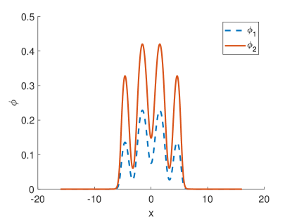
(a) $\alpha=0.2$

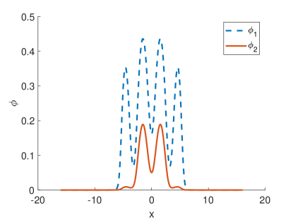
(b) $\alpha=0.9$

Figure 1: Wave functions of the ground state of a spin-1/2 BEC for Example 1 with $\beta=100$, i.e., $\phi_{1}(x)$ (dash line) and $\phi_{2}(x)$ (solid line). The left is for $\alpha=0.2$, and the right is for $\alpha=0.9$.

6.3 Application in anti-ferromagnetic spin-1 BECs

In this subsection, we apply the ANNI and ALM with the Fourier pseudo-spectral scheme to compute the ground state of the spin-1 BEC in 2D and 3D cases with different interactions. We also compare them with the ARNT method [25].

The specific formulation of the minimization problem for computing the ground states of spin-1 BECs is stated as follows [25, 16]:

$$\min{} E(\Phi)=\int_{\mathbb{R}^{d}}\left\{\sum_{l=-1}^{1}\left(\frac{1}{2}|\nabla\phi_{l}|^{2}+(V(\mathbf{x})-pl+ql^{2})|\phi_{l}|^{2}\right)+\frac{\beta_{0}}{2}|\Phi|^{4}+\frac{\beta_{1}}{2}|\mathbf{F}|^{2}\right\}d\mathbf{x}$$ (21)

s.t. $$\int_{\mathbb{R}^{d}}\sum_{l=-1}^{1}|\phi_{l}(\mathbf{x})|^{2}d\mathbf{x}=1,~{}\int_{\mathbb{R}^{d}}\sum_{l=-1}^{1}l|\phi_{l}(\mathbf{x})|^{2}d\mathbf{x}=M,$$

where $M\in[-1,1]$ is the magnetization constraint, and $p,~{}q$ are the linear and quadratic Zeeman engergy shift. $\mathbf{F}:=\mathbf{F}(\Phi)=(\Phi^{*}f_{x}\Phi,\Phi^{*}f_{y}\Phi,\Phi^{*}f_{z}\Phi)^{T}$ is the spin vector where $f_{x},f_{y},f_{z}$ are Hermitian spin-1 matrices. $\beta_{0}$ and $\beta_{1}$ are density-dependent and spin-dependent interaction strength, respectively. According to [16, 19], when $q=0$, $M\in(-1,1)$, for the anti-ferromagnatic system $\beta_{1}>0$, (21) can be reduced to the two-component BEC problem as (1) with

$$\beta_{11}=\beta_{22}=\beta_{0}+\beta_{1},~{}\beta_{12}=\beta_{0}-\beta_{1},~{}\alpha=\frac{1+M}{2}.$$

Hence, we can apply our algorithms to this kind of special anti-ferromagnetic spin-1 BECs. In all examples, we take $p=0$. Please refer [25, 16] for the detailed Fourier pseudo-spectral discretization procedure transforming (1) to the finite-dimensional optimization problem. In this way, $A_{1}$ and $A_{2}$ in (2) are positive definite Hermitian matrices instead of $M$-matrices.

Example 2.

The following cases are considered:

• 2D, $V(x,y)=\frac{1}{2}(x^{2}+y^{2})+10[\sin^{2}(\frac{\pi x}{2})+\sin^{2}(\frac{\pi y}{2})]$, $n=2^{9}$.

• 3D, $V(x,y)=\frac{1}{2}(x^{2}+y^{2}+z^{2})+100[\sin^{2}(\frac{\pi x}{2})+\sin^{2}(\frac{\pi y}{2})+\sin^{2}(\frac{\pi z}{2})]$, $n=2^{7}$, $U=[-2,2]^{3}$.

For Example 2, Tables 2 and 3 report the results obtained by ANNI, ALM and ARNT with different $\beta_{0}$, $\beta_{1}$ and computational domains in 2D and 3D cases. In general, ANNI shows the best performance taking the time cost and total iteration numbers into consideration.

However, although ANNI has the posibility to acheive a quadratically convergence, it is not as efficient as expected when computing (21) over relative large computational domains. Figure 4 depicts different convergence behaviour of ANNI in the best and worst cases. Possible explanations for this phenomenon may be that the main linear system involving $J_{\mathbf{v}}(\mathbf{u},\lambda)$ is computed by Newton-CG in an inexact iteration way, or different condition numbers of $J_{\mathbf{v}}(\mathbf{u},\lambda)$ influence the convergence rate. It is worthwhile to find better preconditioners and linear system solvers, as well as other acceleration technique, which beyond the scope of this article. We remark that for relative weak interactions, for which a relative small computational domain is enough, ANNI performs particular well.

Table 2: Numerical results of spin-1 BECs in 2D

	ANNI				ALM				ARNT
$M$	f	nrmG	Iter	CPU(s)	f	nrmG	Iter	CPU(s)	f	nrmG	Iter	CPU(s)
$U=[-4,4]^{2},~{}\beta_{0}=3,\beta_{1}=1$
0.0	7.5123	1.4e-7	10	12.5652	7.5123	5.8e-7	9(162)	19.9461	7.5123	1.0e-6	4(626)	77.8236
0.2	7.5185	1.5e-7	10	12.5625	7.5185	5.6e-7	8(156)	19.7131	7.5185	3.8e-6	4(1044)	139.6554
0.5	7.5547	7.9e-8	9	10.9107	7.5547	7.1e-7	5(134)	15.7645	7.5547	1.4e-6	4(996)	144.5748
0.9	7.6712	7.3e-7	6	6.1135	7.6712	9.8e-7	3(108)	11.9853	7.6712	9.6e-7	4(935)	124.6696
$U=[-4,4]^{2},~{}\beta_{0}=300,\beta_{1}=100$
0.0	15.1616	1.1e-6	10	10.4377	15.1616	6.5e-7	14(131)	12.7836	15.1616	7.2e-6	4(498)	74.1130
0.2	15.2050	1.8e-6	10	10.1560	15.2050	3.9e-7	13(131)	12.2299	15.2050	1.7e-6	4(848)	127.6096
0.5	15.4366	8.1e-7	11	10.4164	15.4366	3.2e-7	13(134)	13.1036	15.4366	3.0e-6	4(689)	101.8221
0.9	16.1122	2.8e-6	10	11.6454	16.1122	9.0e-7	9(112)	11.6300	16.1122	9.6e-6	3(654)	97.2169
$U=[-8,8]^{2},~{}\beta_{0}=3,\beta_{1}=1$
0.0	7.5123	9.2e-5	8	12.8766	7.5123	5.8e-7	9(193)	28.3537	7.5123	3.5e-6	3(230)	39.9724
0.2	7.5185	1.5e-4	8	14.7473	7.5185	5.9e-7	8(184)	29.2379	7.5185	9.9e-7	4(503)	83.0241
0.5	7.5547	4.0e-5	8	14.7459	7.5547	6.6e-7	5(161)	22.2054	7.5547	2.7e-6	4(553)	78.1469
0.9	7.6712	7.3e-7	6	11.2489	7.6712	9.9e-7	3(134)	18.0191	7.6712	1.0e-6	4(371)	59.9707
$U=[-8,8]^{2},~{}\beta_{0}=300,\beta_{1}=100$
0.0	15.1032	8.1e-6	20	18.0925	15.1032	9.7e-7	11(152)	14.8974	15.1032	3.4e-6	3(235)	36.3426
0.2	15.1411	7.8e-6	22	19.7596	15.1411	9.8e-7	10(147)	14.5061	15.1411	5.1e-6	4(278)	46.2050
0.5	15.3436	7.2e-6	19	19.3722	15.3436	7.2e-7	10(147)	16.7837	15.3436	2.0e-6	4(376)	49.8391
0.9	15.9621	4.0e-6	44	34.1306	15.9621	9.7e-7	9(138)	16.4249	15.9621	4.1e-6	3(357)	55.0067
$U=[-16,16]^{2},~{}\beta_{0}=0.3,\beta_{1}=0.1$
0.0	6.5529	2.8e-6	13	19.6986	6.5529	2.8e-7	3(187)	35.3465	6.5529	9.9e-7	3(84)	22.9629
0.2	6.5546	3.1e-6	12	17.9191	6.5546	4.4e-7	4(191)	36.3004	6.5546	1.2e-6	3(131)	26.7889
0.5	6.5639	3.4e-6	17	31.9996	6.5639	5.5e-7	4(350)	63.5545	6.5639	1.1e-6	3(133)	26.1538
0.9	6.5886	4.2e-6	21	33.5341	6.5886	1.1e-7	3(524)	110.0172	6.5886	9.1e-7	3(119)	25.6818
$U=[-16,16]^{2},~{}\beta_{0}=300,\beta_{1}=100$
0.0	15.1032	7.8e-6	33	42.2618	15.1032	6.9e-7	10(215)	28.4436	15.1032	1.6e-5	3(105)	23.0154
0.2	15.1411	7.7e-6	43	49.3045	15.1411	8.0e-7	10(214)	28.4626	15.1411	2.1e-6	3(128)	23.5979
0.5	15.3436	6.2e-6	68	75.0878	15.3436	6.6e-7	11(256)	35.5117	15.3436	2.1e-6	3(196)	31.8997
0.9	15.9621	4.6e-6	55	66.6906	15.9621	6.5e-7	9(245)	33.0279	15.9621	1.8e-6	3(159)	31.0307

Table 3: Numerical results of spin-1 BECs in 3D

	ANNI				ALM				ARNT
$M$	f	nrmG	Iter	CPU(s)	f	nrmG	Iter	CPU(s)	f	nrmG	Iter	CPU(s)
$\beta_{0}=3,\beta_{1}=1$
0.0	35.5665	5.1e-7	13	233.4272	35.5665	6.9e-7	12(225)	440.0288	35.5665	9.3e-7	3(274)	356.9422
0.2	35.5819	3.6e-7	14	253.4610	35.5819	2.5e-7	15(239)	471.3025	35.5819	8.9e-7	3(333)	625.0140
0.5	35.6633	8.3e-7	45	801.9380	35.6633	9.9e-7	10(167)	254.5624	35.6633	9.6e-7	4(449)	703.8577
0.9	35.9170	1.3e-4	33	533.7613	35.9170	5.6e-7	9(201)	388.2164	35.9170	2.2e-5	4(449)	603.3110
$\beta_{0}=300,\beta_{1}=100$
0.0	72.5380	7.0e-6	8	76.1013	72.5380	3.9e-5	100(348)	308.4463	72.5380	6.8e-6	3(52)	129.9103
0.2	72.7579	4.2e-6	8	86.6609	72.7579	3.8e-7	14(130)	83.0561	72.7579	6.5e-6	3(81)	165.0894
0.5	73.9404	5.9e-6	9	90.0765	73.9404	9.5e-7	30(169)	136.8451	73.9404	6.0e-6	3(97)	143.0615
0.9	77.4006	1.4e-5	10	101.6899	77.4006	6.7e-7	17(134)	118.9649	77.4006	6.0e-6	3(168)	238.8989

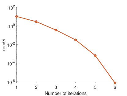
(a) converge quadratically

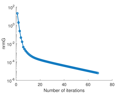
(b) converge rather slowly

Table 4: The convergence behaviour of ANNI. The left is for the case of $U=[-8,8]^{2},~{}\beta_{0}=3,~{}\beta_{1}=1,~{}M=0.9$. In this case, ANNI shows quadratically convergence. The right is for the case of $U=[-16,16]^{2},~{}\beta_{0}=300,~{}\beta_{1}=100,~{}M=0.5$. In this case, ANNI converges rather slowly.

6.4 Application in spin-2 BECs

Consider the ground state of the following spin-2 multi-component BEC problem [25, 16]:

$$\min{} E(\Phi)=\int_{\mathbb{R}^{d}}\left\{\sum_{l=-2}^{2}\left(\frac{1}{2}|\nabla\phi_{l}|^{2}+(V(\mathbf{x})-pl+ql^{2})|\phi_{l}|^{2}\right)+\frac{\beta_{0}}{2}|\Phi|^{4}+\frac{\beta_{1}}{2}|\mathbf{F}|^{2}+\frac{\beta_{2}}{2}|A_{00}|^{2}\right\}d\mathbf{x}$$ (22)

$$\rm{s.t.}{} \int_{\mathbb{R}^{d}}\sum_{l=-2}^{2}|\phi_{l}|^{2}d\mathbf{x}=1,\quad\int_{\mathbb{R}^{d}}\sum_{l=-2}^{2}l|\phi_{l}|^{2}d\mathbf{x}=M,$$

where $M\in[-2,2]$ is the magnetization constraint, $\beta_{2}$ is the spin-singlet interaction strength and all the other parameters $p,q,\beta_{0}$ and $\beta_{1}$ are the same as those in the spin-1 case, $\mathbf{F}$ is the spin vector defined by spin-2 matrices similar to $\mathbf{F}$ for spin-1 BECs. $A_{00}:=A_{00}(\Phi)=\Phi^{T}A\Phi$, where the matrix

$$A=\frac{1}{\sqrt{5}}\begin{bmatrix}0&0&0&0&1\\ 0&0&0&-1&0\\ 0&0&1&0&0\\ 0&-1&0&0&0\\ 1&0&0&0&0\end{bmatrix}.$$

According to [16, 19], for the special case with $\beta_{2}<0$, $\beta_{1}>\frac{\beta_{2}}{20}$, (22) can be transformed to an equivalent two-component BEC problem (1) with

$$\beta_{11}=\beta_{22}=\beta_{0}+4\beta_{1},~{}\beta_{12}=\beta_{0}-4\beta_{1}+\frac{2}{5}\beta_{2},~{}\alpha=\frac{2+M}{4}.$$

For the spin-2 BEC problem, we also discretize it by the Fourier pseudo-spectral scheme.

Example 3.

The following cases are considered:

• 2D, $V(x,y)=\frac{1}{2}(x^{2}+y^{2})+10[\sin^{2}(\frac{\pi x}{2})+\sin^{2}(\frac{\pi y}{2})]$, $n=2^{9}$.

• 3D, $V(x,y)=\frac{1}{2}(x^{2}+y^{2}+z^{2})+100[\sin^{2}(\frac{\pi x}{2})+\sin^{2}(\frac{\pi y}{2})+\sin^{2}(\frac{\pi z}{2})]$, $n=2^{7}$, $U=[-2,2]^{3}$.

Comparison results for spin-2 BECs are summarized in Tables 5 and 6. The numerical results are similar to those for the spin-1 cases. ANNI performs particular well in the case of relative weak interactions and small computational domains.

Table 5: Numerical results of spin-2 BECs in 2D

	ANNI				ALM				ARNT
$M$	f	nrmG	Iter	CPU(s)	f	nrmG	Iter	CPU(s)	f	nrmG	Iter	CPU(s)
$U=[-6,6]^{2},~{}\beta_{0}=243,\beta_{1}=12.1,\beta_{3}=-13$
0.0	14.3386	2.3e-6	13	16.0472	14.3386	7.4e-7	18(194)	19.8875	14.3435	2.4e-6	3(118)	13.5246
0.5	14.3730	2.2e-6	14	17.8339	14.3730	5.4e-7	21(195)	21.5416	14.3730	1.7e-6	3(254)	21.6360
1.5	14.6754	4.3e-6	14	15.2931	14.6754	8.5e-7	14(156)	16.8969	14.6754	2.6e-6	3(241)	23.2947
$U=[-8,8]^{2},~{}\beta_{0}=243,\beta_{1}=12.1,\beta_{3}=-13$
0.0	14.3386	7.9e-6	53	35.0952	14.3386	7.3e-7	18(205)	23.3918	14.3386	1.8e-6	3(99)	11.7415
0.5	14.3730	6.8e-6	80	50.9293	14.3730	9.0e-7	17(198)	22.8233	14.3730	1.5e-6	3(179)	19.0724
1.5	14.6754	5.7e-6	47	36.9902	14.6754	7.7e-8	15(173)	19.6615	14.6754	1.7e-6	3(204)	17.8940
$U=[-8,8]^{2},~{}\beta_{0}=5,\beta_{1}=1,\beta_{2}=-1$
0.0	7.8431	3.4e-6	12	14.8751	7.8431	5.2e-7	5(132)	14.9051	7.8431	1.6e-6	3(126)	15.2849
0.5	7.8648	3.9e-6	13	15.0635	7.8648	6.7e-7	6(138)	16.4655	7.8648	1.3e-6	3(123)	15.8822
1.5	8.0695	4.3e-6	11	13.1936	8.0695	7.4e-7	4(135)	15.2861	8.0695	1.4e-6	3(187)	18.9219
$U=[-8,8]^{2},~{}\beta_{0}=500,\beta_{1}=100,\beta_{2}=-100$
0.0	17.0099	1.1e-6	8	11.6832	17.0099	1.6e-7	6(101)	9.5828	17.0099	1.7e-6	3(148)	14.5422
0.5	17.1973	1.4e-7	8	9.5551	17.1973	5.3e-8	7(99)	9.6300	17.1973	1.9e-6	3(147)	15.9410
1.5	18.7462	4.2e-6	12	12.1355	18.7462	1.9e-7	6(100)	9.8091	18.7462	2.5e-6	3(147)	15.9410

Table 6: Numerical results of spin-2 BECs in 3D

	ANNI				ALM				ARNT
$M$	f	nrmG	Iter	CPU(s)	f	nrmG	Iter	CPU(s)	f	nrmG	Iter	CPU(s)
$\beta_{0}=243,\beta_{1}=12.1,\beta_{2}=-13$
0.0	68.1976	7.1e-6	11	99.6106	68.1976	7.0e-7	15(164)	224.0905	68.1976	3.7e-6	3(60)	223.7610
0.5	68.4124	8.7e-6	12	119.5205	68.4124	9.4e-7	15(167)	175.0873	68.4124	3.9e-6	3(109)	314.6881
1.5	70.2096	2.0e-5	13	143.3075	70.2096	2.8e-7	18(167)	309.7922	70.2096	4.1e-6	3(174)	409.1931
$\beta_{0}=5,\beta_{1}=1,\beta_{2}=-1$
0.0	36.3574	8.5e-7	8	117.3229	36.3574	6.9e-7	5(138)	391.8690	36.3574	7.4e-6	3(189)	997.0649
0.5	36.4399	6.7e-7	11	181.8388	36.4399	6.4e-7	5(129)	355.2176	36.4399	7.1e-6	3(261)	1158.5054
1.5	37.1318	2.0e-7	18	234.6593	37.1318	9.2e-7	3(121)	244.5190	37.1318	6.3e-6	3(220)	1098.9110

7 Conclusion

In this paper, the discretized energy functional minimization problem of a class of special multi-component BECs was considered. The original problem was reduced to a structured nonconvex optimization problem over spherical constraints. We apply the alternating minimization scheme to solve it. In particular, an easy-to-implement alternating Newton-Noda iteration (ANNI) with the one-step modifined NNI in each inner iteration was designed to solve the discretized problem. The global convergence is guaranteed based on the sufficient descent property. We also proved that the proposed algorithms are positivity preserveing under mild conditions. Furthermore, ANNI can be applied to a class of more general multi-block nonconvex minimization problems.

Numerical results on different multi-component BECs are provided to confirm our theoretical results and demonstrate the efficiency of ANNI, especially for the weak interaction cases, for which a relative small computational domain is enough. In this case, ANNI shows the possibility to converge quadratically. However, the explicit convergence rate analysis with respect to different $J_{\mathbf{v}}(\mathbf{u},\lambda)$ needs future research. It is still an interesting problem to study further whether to improve the performance of ANNI when the computational domain is rather large via better preconditioners, other efficient linear system solvers or approximating $J_{\mathbf{v}}(\mathbf{u},\lambda)$ by well-conditioned matrices.

References

• [1] Mike H Anderson, Jason R Ensher, Michael R Matthews, Carl E Wieman, and Eric A Cornell. Observation of bose-einstein condensation in a dilute atomic vapor. Science, 269(5221):198–201, 1995.
• [2] Kendall B Davis, M-O Mewes, Michael R Andrews, Nicolaas J van Druten, Dallin S Durfee, DM Kurn, and Wolfgang Ketterle. Bose-einstein condensation in a gas of sodium atoms. Phys. Rev. Lett., 75(22):3969, 1995.
• [3] Cl C Bradley, CA Sackett, JJ Tollett, and Randall G Hulet. Evidence of bose-einstein condensation in an atomic gas with attractive interactions. Phys. Rev. Lett., 75(9):1687, 1995.
• [4] Jens O Andersen. Theory of the weakly interacting bose gas. Rev. Mod. Phys., 76(2):599, 2004.
• [5] Franco Dalfovo, Stefano Giorgini, Lev P Pitaevskii, and Sandro Stringari. Theory of bose-einstein condensation in trapped gases. Rev. Mod. Phys., 71(3):463, 1999.
• [6] Weizhu Bao and Weijun Tang. Ground-state solution of bose–einstein condensate by directly minimizing the energy functional. J. Comput. Phys., 187(1):230–254, 2003.
• [7] Eric Cancès, Rachida Chakir, and Yvon Maday. Numerical analysis of nonlinear eigenvalue problems. J. Sci. Comput., 45(1-3):90–117, 2010.
• [8] Weizhu Bao and Yongyong Cai. Mathematical theory and numerical methods for bose-einstein condensation. Kinet. Relat. Models, 6(1):1–135, 2013.
• [9] Xavier Antoine, Antoine Levitt, and Qinglin Tang. Efficient spectral computation of the stationary states of rotating bose–einstein condensates by preconditioned nonlinear conjugate gradient methods. J. Comput. Phys., 343:92–109, 2017.
• [10] CJ Myatt, EA Burt, RW Ghrist, Eric A Cornell, and CE Wieman. Production of two overlapping bose-einstein condensates by sympathetic cooling. Phys. Rev. Lett., 78(4):586, 1997.
• [11] DM Stamper-Kurn, MR Andrews, AP Chikkatur, Stenger Inouye, H-J Miesner, J Stenger, and W Ketterle. Optical confinement of a bose-einstein condensate. Phys. Rev. Lett., 80(10):2027, 1998.
• [12] MD Barrett, JA Sauer, and MS Chapman. All-optical formation of an atomic bose-einstein condensate. Phys. Rev. Lett., 87(1):010404, 2001.
• [13] M-S Chang, CD Hamley, MD Barrett, JA Sauer, KM Fortier, W Zhang, L You, and MS Chapman. Observation of spinor dynamics in optically trapped rb 87 bose-einstein condensates. Phys. Rev. Lett., 92(14):140403, 2004.
• [14] Yuki Kawaguchi and Masahito Ueda. Spinor bose–einstein condensates. Phys. Rep., 520(5):253–381, 2012.
• [15] Dan M Stamper-Kurn and Masahito Ueda. Spinor bose gases: Symmetries, magnetism, and quantum dynamics. Rev. Mod. Phys., 85(3):1191, 2013.
• [16] Weizhu Bao and Yongyong Cai. Mathematical models and numerical methods for spinor bose-einstein condensates. Commun. Comput. Phys., 24(4):899–965, 2018.
• [17] Weizhu Bao. Ground states and dynamics of multicomponent bose–einstein condensates. Multiscale Model. Simul., 2(2):210–236, 2004.
• [18] I Chern, Liren Lin, et al. A kinetic energy reduction technique and characterizations of the ground states of spin-1 bose-einstein condensates. Discrete and Continuous Dynamical Systems, Ser. B, 2014.
• [19] Weizhu Bao, I-Liang Chern, and Yanzhi Zhang. Efficient numerical methods for computing ground states of spin-1 bose–einstein condensates based on their characterizations. J. Comput. Phys., 253:189–208, 2013.
• [20] Shu-Ming Chang, Wen-Wei Lin, and Shih-Feng Shieh. Gauss–seidel-type methods for energy states of a multi-component bose–einstein condensate. J. Comput. Phys., 202(1):367–390, 2005.
• [21] Weizhu Bao and Hanquan Wang. A mass and magnetization conservative and energy-diminishing numerical method for computing ground state of spin-1 bose–einstein condensates. SIAM J. Numer. Anal., 45(5):2177–2200, 2007.
• [22] Weizhu Bao and Fong Yin Lim. Computing ground states of spin-1 bose–einstein condensates by the normalized gradient flow. SIAM J. Sci. Comput., 30(4):1925–1948, 2008.
• [23] Hanquan Wang. A projection gradient method for computing ground state of spin-2 bose–einstein condensates. J. Comput. Phys., 274:473–488, 2014.
• [24] P-A Absil, Robert Mahony, and Rodolphe Sepulchre. Optimization algorithms on matrix manifolds. Princeton University Press, 2008.
• [25] Tonghua Tian, Yongyong Cai, Xinming Wu, and Zaiwen Wen. Ground states of spin-f bose–einstein condensates. SIAM J. Sci. Comput., 42(4):B983–B1013, 2020.
• [26] Ching-Sung Liu. A positivity preserving iterative method for finding the ground states of saturable nonlinear schrödinger equations. J. Sci. Comput., 84(3):1–22, 2020.
• [27] Chang-En Du and Ching-Sung Liu. Newton–noda iteration for computing the ground states of nonlinear schrödinger equations. SIAM J. Sci. Comput., 44(4):A2370–A2385, 2022.
• [28] Pengfei Huang and Qingzhi Yang. Newton-based methods for finding the positive ground state of gross-pitaevskii equations. J. Sci. Comput., 90(1):49, 2022.
• [29] Xinming Wu, Zaiwen Wen, and Weizhu Bao. A regularized newton method for computing ground states of bose–einstein condensates. J. Sci. Comput., 73:303–329, 2017.
• [30] Ching-Sung Liu, Chun-Hua Guo, and Wen-Wei Lin. A positivity preserving inverse iteration for finding the perron pair of an irreducible nonnegative third order tensor. SIAM J. Matrix Anal. Appl., 37(3):911–932, 2016.
• [31] Richard S Varga. Matrix Iterative analysis. Springer, New York, 2000.
• [32] Roger A Horn and Charles R Johnson. Matrix analysis. Cambridge university press, 2012.
• [33] Pengfei Huang, Qingzhi Yang, and Yuning Yang. Finding the global optimum of a class of quartic minimization problem. Comput. Optim. Appl., 81(3):923–954, 2022.
• [34] Weizhu Bao and Xinran Ruan. Computing ground states of bose–einstein condensates with higher order interaction via a regularized density function formulation. SIAM J. Sci. Comput., 41(6):B1284–B1309, 2019.
• [35] Gene H Golub and Charles F Van Loan. Matrix computations. JHU press, 2013.
• [36] Jianke Yang. Nonlinear waves in integrable and nonintegrable systems. SIAM, 2010.
• [37] Weizhu Bao and Yongyong Cai. Ground states of two-component bose-einstein condensates with an internal atomic josephson junction. E Asian J. Appl. Math., 1(1):49–81, 2011.