Revisiting Permutation Symmetry for Merging Models between Different Datasets

Abstract

Model merging is a new approach to creating a new model by combining the weights of different trained models. Previous studies report that model merging works well for models trained on a single dataset with different random seeds, while model merging between different datasets is difficult. Merging knowledge from different datasets has practical significance, but it has not been well investigated. In this paper, we investigate the properties of merging models between different datasets. Through theoretical and empirical analyses, we find that the accuracy of the merged model decreases more significantly as the datasets diverge more and that the different loss landscapes for each dataset make model merging between different datasets difficult. We also show that merged models require datasets for merging in order to achieve a high accuracy. Furthermore, we show that condensed datasets created by dataset condensation can be used as substitutes for the original datasets when merging models. We conduct experiments for model merging between different datasets. When merging between MNIST and Fashion-MNIST models, the accuracy significantly improves by $28\%$ using the dataset and $25\%$ using the condensed dataset compared with not using the dataset.

1 Introduction

Model merging (Leontev et al., 2020; Singh and Jaggi, 2020; Ainsworth et al., 2023) is an approach to creating a new model that combines the weights contained in different deep neural networks (DNNs). DNNs are nonlinear, thus merging models was thought to be difficult. The recent discovery of a DNN property called Linear Mode Connectivity (LMC) (Frankle et al., 2020) brings us closer to the realization of model merging. The LMC means that if the optimal weights of two DNNs are given, they are trapped in the same basin of the loss landscape. This means that the model created from the average of these weights has a high accuracy since there is no loss barrier between the weights with LMC. Entezari et al. (2021) and Ainsworth et al. (2023) report that two networks trained with different random seeds have an LMC if the neurons are properly aligned.

Previous studies (Ainsworth et al., 2023; Leontev et al., 2020; Singh and Jaggi, 2020) report that model merging works well for models trained on a single dataset with different random seeds. On the other hand, it has been reported that models trained on different datasets are difficult to merge. Merging knowledge from different datasets has practical significance. Thus, this study addresses two research questions.

• RQ1: How difficult does model merging become as datasets become more different?

• RQ2: What makes model merging between different datasets more difficult than model merging with the same dataset?

To address RQ1, we evaluate the accuracy of a series of merging models while incrementally increasing the gap between datasets. In this paper, we introduce the metric of the gap between datasets called flipped accuracy, which is the average of the accuracy of Model A on Dataset B and Model B on Dataset A. The experimental results indicate that model merging becomes more difficult as flipped accuracy decreases. Next, to address RQ2, we analyze the loss landscape theoretically and experimentally. We found that model merging between the same datasets can achieve good performance since the optimal weights are the same, but different datasets have different optimal weights and loss landscapes, which create a loss barrier and makes model merging difficult (see Fig. 1).

In this paper, we attempt to effectively merge models between different optimal weights. Existing research (Entezari et al., 2021; Ainsworth et al., 2023) demonstrates that suitably aligning neurons and averaging the weights to merge models can effectively minimize the loss. In single dataset setting, aligning neurons only with weights can achieve effective model merging without external information such as gradients and datasets (Ainsworth et al., 2023) since the optimal weights are the same. However, we can expect that model merging in different dataset setting is hard to be done with only weight due to the mismatch of the loss landscapes between datasets as discussed in the previous paragraph. Thus, the following research question naturally arises.

• RQ3: What information is needed to achieve effective model merging between different datasets?

To answer RQ3, we investigate three categories of aligning methods: (i) align neurons on the basis of their weights, (ii) align neurons using both their weights and gradients, (iii) align neurons considering their weights and dataset information. The latter of these three categories requires more information. Through generating various alignments without a dataset, we found that the criteria from weights and gradients are not positively correlated with the loss on the mixed dataset. On the other hand, the alignment criteria created from the dataset is correlated well with the loss on the mixed dataset. In fact, in many cases of model merging between different datasets, aligning with dataset information greatly improves the accuracy of model merging. Therefore, we conclude that a mixed dataset is currently required for effectively merging models between different datasets.

The fact that all data points are required for effective model merging is a major constraint in terms of the cost of data storage. Thus, we further investigate a fourth research question.

• RQ4: Can we reduce the data points required for effective model merging?

To answer RQ4, we propose merging models using a condensed dataset instead of a real dataset. Dataset condensation (Zhao et al., 2021) is a method of distilling the knowledge of a dataset into small numbers of data points to achieve high accuracy with less data. The proposed method can reduce the number of data points required for model merging by dataset condensation. Our experiments show that model merging with a condensed dataset is competitive with the baseline. In particular, the model merging using the condensed dataset has better accuracy than models trained from scratch by using the union set of the condensed dataset. This is because the proposed method has the advantage of using the optimal weight information of each dataset. The neuron alignment operation keeps a low loss value on the mixed dataset, since its alignment keeps the optimized loss value on the individual datasets. Our main contributions are summarized as follows:

• We confirm that model merging becomes more difficult as datasets become more different.

• We reveal that the difficulty of model merging is caused by the loss landscapes of each dataset being mismatched as datasets become more different.

• We find that dataset is currently required for effectively merging models between different datasets.

• We propose a method of model merging by using a condensed dataset instead of a real dataset. This approach greatly reduces the number of data points required.

2 Preliminary

We present a short preliminary for model merging. First, we formulate the problem of model merging extended between different datasets. Then, we introduce permutation symmetry of neurons in DNN, which plays an important role in model merging. Finally, we introduce existing methods for model merging.

2.1 Goal of Model Merging

Let us consider merging the model parameters $\mathbf{w_{A}}$ and $\mathbf{w_{B}}$ trained on Datasets $D_{A}$ and $D_{B}$ respectively. Mixed dataset $D_{AB}=D_{A}\cup D_{B}$ is defined as the union of the two datasets. The goal of model merging is to obtain operator $\star$ as follows

$$\mathcal{L}_{AB}\left(\mathbf{w_{AB}}\right)\simeq\mathcal{L}_{AB}\left(\mathbf{w_{A}}\star\mathbf{w_{B}}\right),$$ (1)

where $\mathbf{w_{AB}}=\operatorname*{arg\,min}_{\mathbf{w}}\mathcal{L}_{AB}\left(\mathbf{w}\right)$, $\mathbf{w_{A}}=\operatorname*{arg\,min}_{\mathbf{w}}\mathcal{L}_{A}\left(\mathbf{w}\right)$, $\mathbf{w_{B}}=\operatorname*{arg\,min}_{\mathbf{w}}\mathcal{L}_{B}\left(\mathbf{w}\right)$. $\mathcal{L}_{A}\left(\mathbf{w}\right)$ denotes loss on $D_{A}$ as $\mathcal{L}_{A}=E_{p_{D_{A}}\left(y,\mathbf{x}\right)}\left[-\log p\left(y|\mathbf{x},\mathbf{w}\right)\right]$. In this paper we assume for simplicity that Models A and B have the same architecture.

2.2 Permutation Symmetry

DNNs have neuron permutation symmetry, which is realized by rearranging the weights. Neuron permutation symmetry refers to the property that the output remains invariant with respect to the rearrangement of neurons. Let us consider a specific example of a simple feedforward network. Even if we apply a permutation matrix $P_{\ell}$ to the weights of the $\ell$-th layer $\mathbf{w_{\ell}}$, the output remains invariant if we apply the inverse of $P_{\ell}$ in the weights of the $(\ell+1)$-th layer. In other words, $\mathbf{w_{\ell+1}}P_{\ell}^{-1}\sigma\left(P_{\ell}\mathbf{w_{\ell}}\mathbf{x_{\ell}}\right)=\mathbf{w_{\ell+1}}\sigma\left(\mathbf{w_{\ell}}\mathbf{x_{\ell}}\right)$. Here, $\sigma$ represents the activation function, and $\mathbf{x_{\ell}}$ denotes the input of the $\ell$-th layer. By utilizing this freedom of rearrangement, we can permute the weights without changing the loss value.

2.3 Model Merging

Existing research (Entezari et al., 2021; Ainsworth et al., 2023) demonstrates that suitably aligning and averaging the weights to merge models can effectively minimize the loss in a single dataset. The suitable alignment and averaging of the weights is formulated as

$$\mathbf{w_{A}}\star\mathbf{w_{B}}=\left(1-\lambda\right)\mathbf{w_{A}}+\lambda\pi\left(\mathbf{w_{B}}\right),$$ (2)

where $\pi$ is permutation of weights and $\lambda\in\left[0,1\right]$ is constant. We present two methods introduced in Ainsworth et al. (2023).

WM: Weight Matching (WM) permutes the weights to reduce the L2 distance between weights of trained models as

$$\operatorname*{arg\,min}_{\pi}\left\|{\rm vec}\left(\mathbf{w_{A}}\right)-{\rm vec}\left(\pi\left(\mathbf{w_{B}}\right)\right)\right\|^{2}.$$ (3)

This search for permutations can be reduced to a classic linear assignment problem and can be performed quickly. Equation (3) can be optimized using only weight without datasets.

STE: Straight Through Estimator (STE) learns permutations to reduce the loss of parameters after merging as

$$\min_{\mathbf{\tilde{w}_{B}}}\mathcal{L}_{AB}\left(\left(1-\lambda\right)\mathbf{w_{A}}+\lambda{\rm proj}\left(\mathbf{\tilde{w}_{B}}\right)\right),\quad{\rm proj}\left(\mathbf{w}\right)=\operatorname*{arg\,min}_{\pi\left(\mathbf{w_{B}}\right)}\left\|{\rm vec}\left(\mathbf{w}\right)-{\rm vec}\left(\pi\left(\mathbf{w_{B}}\right)\right)\right\|^{2}.$$ (4)

STE requires a dataset to estimate the loss. On model merging between models trained on a single dataset, Ainsworth et al. (2023) reports that WM achieves similar accuracy to STE, despite not using the dataset. Therefore, WM was the main subject of investigation in an existing study (Ainsworth et al., 2023).

3 Model Merging between Different Datasets

In this section, we investigate model merging between different datasets. First, we confirm that model merging becomes more difficult as datasets become more different. Then, we provide an intuitive understanding of model merging between different datasets and identify the causes of merging difficulties. Our investigation shows that datasets are required for effective model merging between different datasets. Finally, we propose a model merging method using dataset condensation that decreases the requirement for real data.

3.1 Datasets Differences Affect the Accuracy of Model Merging

Table 1: Effects of different datasets on WM.

Degree	L2	Barrier	FAcc	Acc (WM)
$90^{\circ}$	$4.03\times 10^{-5}$	1.280	14.79	70.86
$75^{\circ}$	$4.06\times 10^{-5}$	1.098	17.06	74.19
$60^{\circ}$	$4.07\times 10^{-5}$	0.804	26.28	80.33
$45^{\circ}$	$4.05\times 10^{-5}$	0.390	45.96	89.68
$30^{\circ}$	$4.00\times 10^{-5}$	0.217	75.26	94.69
$15^{\circ}$	$3.96\times 10^{-5}$	0.062	95.22	97.53
$0^{\circ}$	$3.84\times 10^{-5}$	0.008	98.47	98.49

In this section, we investigate the impact of different datasets on model merging. To continuously create differences in datasets, we design Rotated-MNIST (RMNIST), which consists of MNIST images rotated by varying angles and conduct model merging experiments between MNIST and RMNIST. RMNIST uses rotations of $0^{\circ}$, $15^{\circ}$, $30^{\circ}$, $45^{\circ}$, $60^{\circ}$, $75^{\circ}$, and $90^{\circ}$. The experimental procedure involves training Model A on MNIST (Dataset A) and Model B on RMNIST (Dataset B), then merging Models A and B using WM and measuring accuracy on a mixed dataset (Dataset AB). Table 1 summarises the results when varying rotation degrees of RMNIST. L2 represents the L2 distance between $\mathbf{w_{A}}$ and $\mathbf{w_{B}}$, and the barrier represents the training loss on Dataset AB at the average of $\mathbf{w_{A}}$ and $\mathbf{w_{B}}$ (the barrier will be introduced in Sec. 3.2). Here, we introduce Flipped Acc (FAcc) as a measure of the difference between datasets. FAcc is defined as the average of Model A’s accuracy on Dataset B and Model B’s accuracy on Dataset A. Table 1 shows that the accuracy of WM decreases as the difference (angle) between the datasets increases. Furthermore, Table 1 also shows that the FAcc decreases as the angle difference increases. This is consistent with the intuition that accuracy decreases when training and test data differ. We found that FAcc is a good indicator for measuring the final accuracy of WM after merging.

3.2 Causes of Difficulties with Model Merging

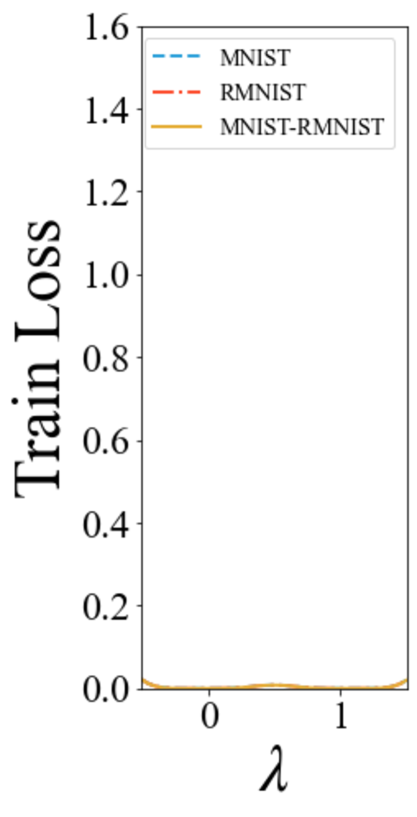
(a) $0^{\circ}$

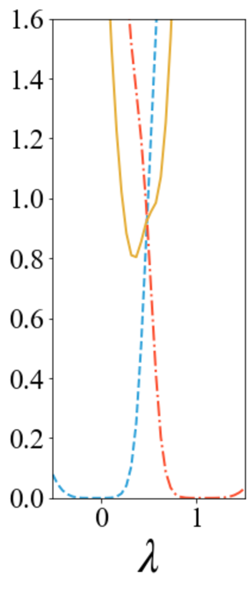
(b) $45^{\circ}$

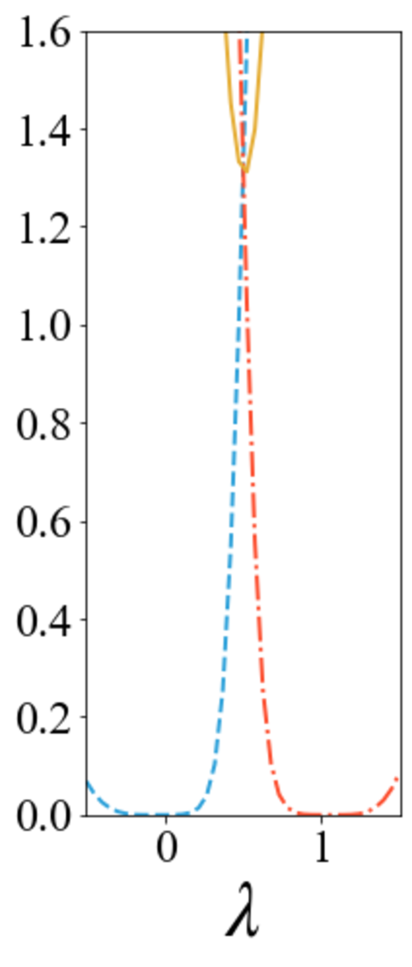
(c) $90^{\circ}$

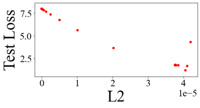
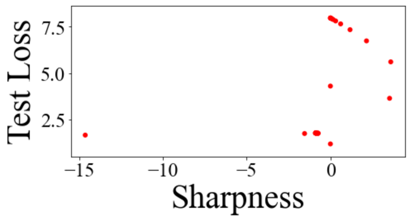
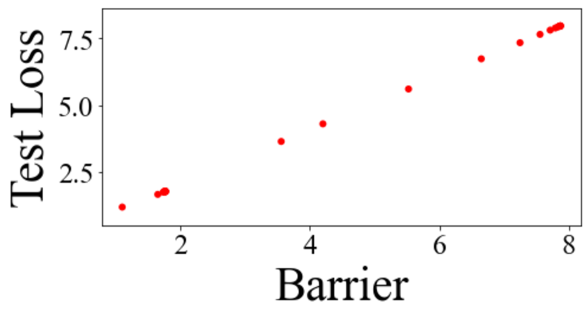
(d) Correlation

Figure 1: (1, 1, 1) show training loss between MNIST and RMNIST. Line differences represent the different datasets to be evaluated, with $\lambda=0$ representing the optimal weights for MNIST and $\lambda=1$ representing the optimal weights for RMNIST. (1) shows the relationship between L2 distance, sharpness, loss barrier and test loss on mixed dataset when various weight permutations are generated between MNIST and RMNIST-90.

This section reveals why model merging between different datasets is difficult. First, we discuss the relationship between the loss landscapes of Datasets A, B, and AB. Since different datasets have different losses, loss landscapes cannot be directly compared between different datasets. Let $p_{D_{AB}}\left(\mathbf{x},y,\alpha\right)=\left(1-\alpha\right)p_{D_{A}}\left(\mathbf{x},y\right)+\alpha p_{D_{B}}\left(\mathbf{x},y\right)$ be the probability distribution of the mixed dataset, where $\alpha\in\left[0,1\right]$ is a constant for the mixing ratio of datasets, for simplicity $\alpha=\frac{1}{2}$ is used. Note that the general $\alpha$ can be discussed in a similar way. The loss is the expected value for the data distribution $\mathcal{L}_{AB}=E_{p_{D_{AB}}\left(y,\mathbf{x}\right)}\left[-\log p\left(y|\mathbf{x},\mathbf{w}\right)\right]$ and can be separated for each dataset by using the linearity of the expectation as follows

$$\mathcal{L}_{AB}\left(\mathbf{w}\right)=\frac{1}{2}\left(\mathcal{L}_{A}\left(\mathbf{w}\right)+\mathcal{L}_{B}\left(\mathbf{w}\right)\right).$$ (5)

Thanks to Eq. (5), we can discuss loss landscapes across different datasets. To achieve effective model merging, the loss barrier $\frac{1}{2}\left(\mathcal{L}_{A}\left(\mathbf{w_{M}}\right)+\mathcal{L}_{B}\left(\mathbf{w_{M}}\right)\right)$ should be small, where $\mathbf{w_{M}}=\left(1-\lambda\right)\mathbf{w_{A}}+\lambda\mathbf{w_{B}}$ is the weight of the merged models. Our theoretical analysis suggests that the optimal weight on a mixed dataset does not necessarily lie on this line segment between $\mathbf{w_{A}}$ and $\mathbf{w_{B}}$ (see Appendix A). However, our experiments show little difference in accuracy between the method that assumes weights on the line segment, as assumed in existing methods, and the method that considers deviations from the line segment (see Appendix C.2). Therefore, we use simple averages. Next, to confirm experimentally that the loss barrier increases as datasets become more different, we show the loss barrier between MNIST and RMNIST in Fig. 1. The blue, red, and yellow lines represent the loss landscapes on MNIST, RMNIST, and MNIST-RMNIST, respectively. The $\lambda=0$ represents the optimal weight on MNIST, and the $\lambda=1$ represents the optimal weight on RMNIST. Figure 1 shows that the loss barrier (yellow line) increases as the angle of MNIST-RMNIST become more different. This is because the more different datasets are, the more the closest optimal weights diverge between different datasets.

3.3 Conditions for Successful Merging

To reduce the loss barrier, we try three methods (Ainsworth et al., 2023) of aligning weights by using different information. The first method is WM to reduce the L2 distance using only weight information. The idea of WM is to reduce the loss barrier by reducing the L2 distance, assuming that there exists an optimal weight such that $\mathbf{w_{A}}=\mathbf{w_{B}}$ even between different datasets. The second method is Flat Weight Matching (FWM) using gradients of weights and weight information. FWM is WM with the regularization to flatten the loss landscape as $\beta\left\|{\rm vec}\left(\mathbf{w_{A}}\right)-{\rm vec}\left(\pi\left(\mathbf{w_{B}}\right)\right)\right\|^{2}+\left(1-\beta\right)\left({\rm vec}\left(\mathbf{w_{A}}\right)-{\rm vec}\left(\pi\left(\mathbf{w_{B}}\right)\right)\right)\left.\frac{\partial\mathcal{L}_{B}}{\partial\mathbf{w}}\right|_{\mathbf{w}=\pi\left(\mathbf{w_{B}}\right)}$, where $\beta$ is constant value and the second term is the regularization term. The idea of FWM is to flatten the loss landscape to reduce the loss barrier at $\mathbf{w_{M}}$ that shift from the optimal weight $\mathbf{w_{A}}$, on the basis of the assumption that $\mathbf{w_{A}}$ and $\mathbf{w_{B}}$ are close but not equal. The third method is STE using the weight and dataset information to reduce the loss barrier directly.

To investigate which information can help in effective merging, Fig. 1 shows the relationship between L2 distance, sharpness, loss barrier and test loss on mixed dataset when various weight permutations are generated between MNIST and RMNIST-90 (for the detailed experimental setup, see the supplementary material). The sharpness of Model A between $\mathbf{w_{A}}$ and $\mathbf{w_{B}}$ is defined as $\left(\mathbf{w_{B}}-\mathbf{w_{A}}\right)\frac{\partial\mathcal{L}_{A}\left(\mathbf{w_{A}}\right)}{\partial\mathbf{w}}$, and the sharpness is defined as the average of sharpness of Model A and B. Figure 1 indicates that the test loss does not become smaller as the L2 distance becomes smaller. This could be because sharpness is not taken into account, even though a decrease in sharpness becomes crucial when the L2 distance is reasonably close. Figure 1 also shows that the sharpness is poorly correlated with test loss of the merged model. This is because loss barriers that deviate from the optimal weights become difficult to estimate when using local gradients on the optimal weights. On the other hand, the loss barrier, which is training loss on mixed datasets, correlates well with test loss. Table 1 also shows that the rank correlation between Acc (WM) and L2 is $-0.75$ and sharpness is $-0.85$, but the loss barrier has a high correlation as $-1$. Therefore, datasets are currently required for effectively merging models between different datasets. We will confirm that STE works effectively between different datasets in Sec. 4. We also conduct experiments with FWM, but the improvement effect on FWM is marginal (see Sec. C.3).

3.4 Model Merging without Real Dataset

Model merging between different datasets requires a smaller loss barrier by using the datasets. However, this is a major constraint on sharing all data in terms of heterogeneous data utilization, data privacy, and data storage cost. To relax this constraint, we propose a method that uses a condensed dataset instead of a real dataset. Dataset condensation is a method for condensing a large dataset into a small set of informative synthetic samples for training deep neural networks from scratch. Various methods have been proposed for dataset condensation, and we use a major method called Gradient Matching (Zhao et al., 2021) in this paper. Gradient Matching creates a condensed dataset so that the gradients of the weights learned on the original dataset match the gradients of the condensed dataset. To summarize the overall procedure for model merging without real data, we first prepare trained models for $D_{A}$ and $D_{B}$ and then perform dataset condensation on $D_{A}$ and $D_{B}$, respectively. Next, we mix Condensed Datasets A and B to create Condensed Dataset AB. Finally, merge models with STE using Condensed Dataset AB instead of real dataset $D_{AB}$.

4 Experiments

Outline. The purpose of the experiment is to confirm that STE is effective for model merging between different datasets and that a reasonable permutation can be achieved even using STE with condensed datasets. The basic experimental procedure is to first train independently on $D_{A}$ and $D_{B}$ to obtain $\mathbf{w_{A}}$ and $\mathbf{w_{B}}$. Then the weights $\mathbf{w_{B}}$ are permuted. Finally, model parameters are merged as $\mathbf{w_{AB}}=\left(1-\lambda\right)\mathbf{w_{A}}+\lambda\pi\left(\mathbf{w_{B}}\right)$ and sliding $\lambda$ to evaluate the accuracy on $D_{AB}$.

Datasets. First, we conduct model merging between different datasets with shared labels, such as MNIST-RMNIST and USPS-MNIST. Both MNIST (LeCun et al., 1998) and USPS (Hull, 1994) are grey-scaled character datasets. Originally, Rotated-MNIST (RMNIST) was a dataset with MNIST rotated by an arbitrary angle, but in this paper, RMNIST is $90^{\circ}$ rotated. When training without data augmentation, models trained on MNIST will have lower accuracy on RMNIST. Next, we experiment with the case of no label sharing as SPLIT-CIFAR10 and MNIST-FMNIST. SPLIT-CIFAR10 divides CIFAR10 (Krizhevsky et al., 2009) into two datasets, one with Labels 0-4 and the other with Labels 5-9. Instead of creating pseudo-different datasets with different numbers of data per label, as in existing studies (Singh and Jaggi, 2020; Ainsworth et al., 2023), this paper has no label leakage between datasets. Leaking labels means that one dataset contains all labels. MNIST-FMNIST merges models between two completely different datasets: MNIST, which includes digit images, and Fashion-MNIST (FMNIST) (Xiao et al., 2017), which includes fashion images.

Setup. We use the same setup for the preprocessing and network architecture as the existing method (Ainsworth et al., 2023). MNIST, USPS, RMNIST, and FMNIST use a fully connected network, and CIFAR10 use ResNet20$\times 16$, which is 16 times wider than ResNet20. This is because existing research has shown that model merging on a single dataset in CIFAR10 cannot be effective unless the width is sufficiently large. Since Batch Normalization is also known to destroy the LMC, we use REPAIR (REnormalizing Permuted Activations for Interpolation Repair) (Jordan et al., 2022) to avoid this. We provide the results of model merging on a single dataset as a preliminary experiment in supplementary material. For data condensation, USPS, MNIST, RMNIST, and FMNIST use Gradient Matching (Zhao et al., 2021) to condense up to 10 data points per class. SPLIT-CIFAR10 uses a public dataset condensed down to 50 images per class using sophisticated methods (Nguyen et al., 2021). For full experimental details, see Sec. B.1.

Baselines. We compare the four methods as a baseline for model merging. Naïve: Simple average method as $\mathbf{w_{AB}}=\left(1-\lambda\right)\mathbf{w_{A}}+\lambda\pi\left(\mathbf{w_{B}}\right)$. WM: The weights are permuted in order to close the L2 distance between the weights of the two models and then averaged. Model Fusion via OT (Singh and Jaggi, 2020): Using OT is sophisticated model merging, with a higher degree of freedom than weights permutation. OT (Tuned) uses $\lambda$ with the highest test accuracy from $\lambda\in\left[0,1\right]$. Since there is a large divergence in performance between $\lambda=0.5$ and Tuned for OT, we include both, while the other methods include results for $\lambda=0.5$.

4.1 Model Merging between Different Datasets.

(a) Full Data

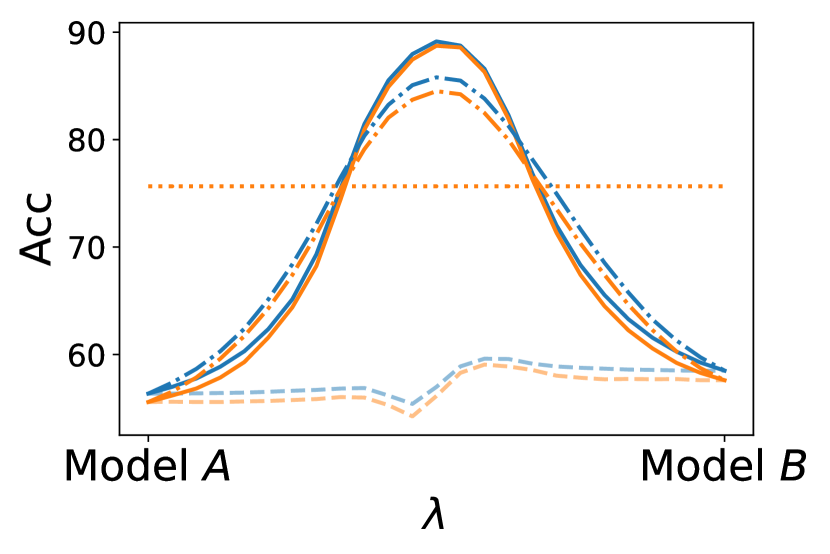
(b) Data Cond-10

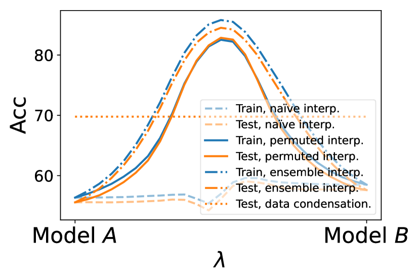
(c) Data Cond-1

Figure 2: Acc on MNIST-RMNIST.

First, for an intuitive understanding of our experiments, we present model merging between MNIST and RMNIST. MNIST as Dataset A and RMNIST as Dataset B, and the models trained on MNIST and RMNIST, respectively, are denoted as Models A and B. Figure 2 shows the accuracy of merged model on $D_{AB}$, which is merged by STE and STE with dataset condensation. Model A ($\lambda=0$) has an accuracy of around $55\%$ on the MNIST and RMNIST mixed dataset, since it is almost $100\%$ accurate on MNIST and $10\%$ on RMNIST. Model B ($\lambda=1$) is similar. As shown in Fig. 2, the permuted (STE) achieves $90\%$ of test accuracy compared to $60\%$ for Naïve. This is surprising as there is an effective weight for model merging in the permutation of neurons.

Table 2: Test Acc (%) on $D_{AB}$.

	MNIST-RMNIST	USPS-MNIST	SPLIT-CIFAR10	MNIST-FMNIST
Model A	55.58	76.04	48.40	53.21
Model B	57.61	62.99	48.90	51.81
Model AB	98.19	96.92	95.63	94.03
Ensemble	84.51	93.46	79.79	75.93
Data Cond	74.47	82.49	38.71	73.28
Naïve	56.14	68.85	10.00	45.75
WM	70.92	84.21	58.91	55.61
OT	37.06	79.20	24.01	24.76
OT (Tuned)	58.57	82.39	46.62	48.10
STE (Full)	93.45	95.18	90.08	83.65
STE (Data Cond)	88.22	92.31	72.15	80.20

Next, similar experiments are conducted across the various datasets. The results are shown in Tab. 2. In the table, Model AB is the oracle model trained with the mixed dataset, while Models A and B are the pre-merging models trained on Datasets A and B, respectively. Ensemble is the average of the predictions of the model. We note that ensemble is compared as a reference due to the doubled inference cost. Compared with Naïve without permutation, STE (Full) achieves higher accuracy in all cases. This shows that the permutation strategy is effective for model merging. Furthermore, STE (Full) outperforms all other baseline methods and ensemble. STE (Full) achieves high accuracy, especially for merging, which is difficult even with OT such as SPLIT-CIFAR10 and MNIST-FMNIST. For model merging on a single dataset, WM and STE (Full) are reported to have similar performance (Ainsworth et al., 2023). However, in model merging between different datasets, we find that STE (Full) significantly outperforms WM. This implies that not only the weights but also the information about the datasets is important when merging between different datasets.

4.2 Model Merging with Data Condensation

To confirm that the data points required for effective model merging can be reduced, we conduct experiments of model merging with condensed datasets. The results on the MNIST-RMNIST are shown in Figs. 2 and 2. Data Cond-10 and Data Cond-1 represent the results using 10 condensed data points per class and 1 condensed data point per class, respectively. In both cases, the proposed method significantly outperforms the naïve method. The proposed method also achieves higher performance than the ensemble, with 10 data points per class. This corresponds to roughly $0.2{\rm\%}\approx\frac{100}{60000}$ for the training dataset. We also compare our approach with the Data Cond method, which trains from scratch using the union set of the condensed dataset. The reason for this comparison is that condensed datasets have fewer data points, and if performance is achieved by training from scratch on the condensed dataset of the two datasets, the benefits of model merging may be reduced. Figures 2 and 2 show that STE with dataset condensation has higher accuracy than the Data Cond method (horizontal dashed line) in both cases. The reason may be that the proposed method uses the optimal weights trained on individual datasets. The proposed method aligns the weights while keeping the optimized loss values for the individual datasets, thus the loss values are kept small on the mixed dataset. Table 2 summarizes comparisons between STE using condensed datasets as STE (Data Cond) and other methods. STE (Data Cond) achieves higher accuracy than other methods except for Ensemble, which has a high inference cost.

4.3 Loss Landscape

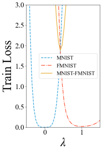
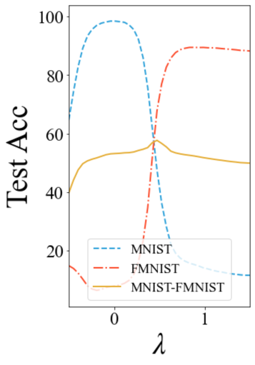
(a) WM

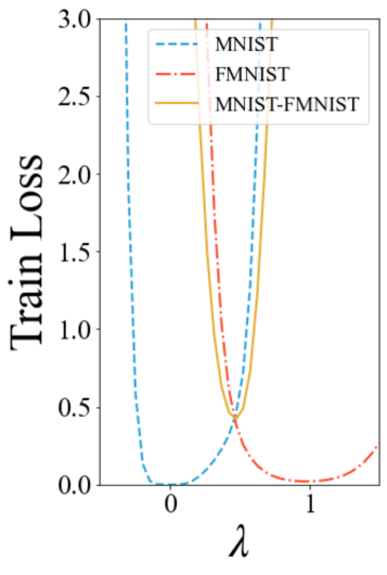
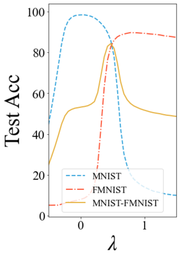
(b) STE

Figure 3: Training loss and test accuracy on MNIST-FMNIST. Line differences represent the different datasets to be evaluated, with $\lambda=0$ representing the optimal weights for MNIST and $\lambda=1$ representing the optimal weights for FMNIST.

We investigate the loss landscape to clarify the differences in the performance of merging models in WM and STE. The investigation uses MNIST-FMNIST, model merging between completely different datasets. Figure 3 shows the loss landscape corresponding to Eq. (2) on the MNIST-FMNIST, with $\lambda=0$ representing the optimal weights for MNIST and $\lambda=1$ representing the optimal weights for FMNIST. Figure 3 shows that for both WM and STE, $\mathbf{w_{AB}}$ and $\mathbf{w_{A}}$ and $\mathbf{w_{B}}$ are in regions close enough that the loss landscape can be considered a convex function. Comparing WM and STE shows that STE has a smaller loss barrier. This is because STE optimizes the direct reduction of loss barrier, which encourages the flatter loss landscapes.

5 Related Work

The purpose of model merging is to create a model combining the knowledge contained in different networks. First, we introduce existing methods that have a similar purpose to model merging and organize the differences with model merging. Then, we introduce LMC, which is closely related to model merging. Finally, the differences with existing model merging research are summarized.

Continuous learning. Continuous learning is a method for learning new knowledge while retaining previously acquired knowledge (Silver et al., 2013). A major strategy in continuous learning is to separate the weights used for learning between Datasets A and B (Kirkpatrick et al., 2017; Mallya and Lazebnik, 2018). In continuous learning, the training of Dataset B requires information from the training of Dataset A, and Model AB is acquired directly. Thus, Dataset B must be re-trained from scratch when merging different pairs of datasets, e.g., Datasets B and C. Model merging, on the other hand, has the advantage of not requiring Models A and B to be re-trained, since it is performed after Datasets A and B have been trained independently.

Federated learning. Federated learning is a learning method without directly sharing the datasets in cases where each training dataset is distributed (McMahan et al., 2017). Federated learning is promising in terms of data privacy, security and the use of heterogeneous data, since datasets are not shared. Instead of sharing data points, gradients of weights for losses are shared. Federated learning has a similar purpose to model merging with condensed datasets, in that it creates a model that can be adapted across the dataset without sharing the raw dataset. In federated learning, the model must be re-trained from scratch when merging different new pairs of datasets. Model merging, on the other hand, does not require re-training.

Ensemble. Ensemble methods (Breiman, 1996; Wolpert, 1992; Schapire, 1999) have a long history and improve the accuracy by taking an average of the predictions of several different models. An ensemble method is used as a baseline for model merging on the single dataset, since an ensemble of models trained with different random seeds can improve the accuracy. As was shown in Sec. 4, the ensemble method works surprisingly well for merging between different datasets. Ensemble methods have disadvantages in terms of computational cost and memory efficiency since they use the predictions of all models in inference. This approach is expensive for many applications where computational resources are limited, especially given the increasingly large size of modern deep learning models.

LMC. The concept of mode connection, where the optimal weights of the scholastic gradient decent (SGD) have connected paths between each other, was introduced by Garipov et al. (2018). Furthermore, Frankle et al. (2020) proposed the LMC and found a relationship between the LMC and the Lottery Hypothesis (Frankle and Carbin, 2019). It has been reported that LMC is valid if the neurons of two networks trained with different random seeds are appropriately permuted (Entezari et al., 2021; Ainsworth et al., 2023). Furthermore, LMC has been reported to be valid between fine-tuning models trained with different random seeds from a single pre-training model (Neyshabur et al., 2020). Thus, LMC has attracted attention as a tool for understanding SGD, the Lottery Hypothesis, and fine-tuning.

Merging Methods. Several methods have been proposed for merging trained models into a single model, such as taking the simple average of the weights (Akhlaghi and Sukhov, 2018), using Hessian information on losses (Leontev et al., 2020; He et al., 2018), using optimal transport (OT) (Singh and Jaggi, 2020), and using neuronal permutations (Ainsworth et al., 2023). These methods focus on model merging on a single dataset or on different datasets that are pseudo-created by changing the proportion of datasets on a label, called a label-leaked dataset. This paper focuses on model merging between different datasets that do not leak labels.

6 Limitations

Our results have several limitations. (1) The analysis in Sec. 3 assumes the existence of optimal weights $\mathbf{w_{A}}$ and $\mathbf{w_{B}}$, which are close enough to be considered convex functions, as shown in Fig. 3. (2) We showed that STE can reach effective permutations experimentally, but there is a large number of permutation patterns, thus there is no theoretical guarantee, and theoretical analysis is a remaining task. (3) Our experiments are limited to image classification between the same model architectures. Adaptation of model merging to natural language datasets and generative models is intriguing applications (e.g. Checkpoint Merger of Stable Diffusion web UI (AUTOMATIC1111, 2022)).

7 Conclusion and Future Work

This paper investigated model merging between different datasets. We found that there is an effective weight for model merging in the permutation of neurons. This finding is a motivation for future research to improve the efficiency of permutation search for model merging between different datasets. Furthermore, we proposed model merging by using a condensed dataset, without sharing all data points. Future work needs to examine whether a condensed dataset protects privacy. In other research directions, the merging between many models is of interest. In DNN training, huge computational costs are being spent to develop huge models to improve accuracy, but this may be a limitation from viewpoint of system energy consumption. Efficient model merging of multiple models could pave the way for new learning methods as (Li et al., 2022) to replace current learning methods where a single data point affects all parameter updates.

Appendix A Theoretical Analysis

A.1 Do Optimal Weights of Dataset AB Lie on a Line Segment between Optimal Weights of Datasets A and B?

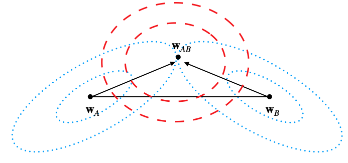
Figure 4: 2D Contours Plot. The relationship between the optimal weights on Datasets A and B before merging and the optimal weights on the optimal datasets after merging. The blue lines represent the contours plot of the loss on Datasets A and B, and the red lines represent the contours plot of the loss on Dataset AB after merging.

In this subsection, we discuss whether the optimal weights in a mixed dataset are on the line between $\mathbf{w_{A}}$ and $\mathbf{w_{B}}$. Let us assume that weight permutation makes $\mathbf{w_{A}}$ and $\mathbf{w_{B}}$ close enough $\mathbf{w}\in\sigma\left(\mathbf{w_{A}},\mathbf{w_{B}}\right)$ and that their respective losses are in a region where they can be regarded as convex functions. This assumption holds with permutation by WM and STE. This is confirmed in Sec. 4.3. In Eq. (5), $\mathcal{L}_{AB}$ is a convex function because it is a convex combination of convex functions $\mathcal{L}_{A}$ and $\mathcal{L}_{B}$, and it is expressed as a quadratic equation around the optimal weight $\mathbf{w_{AB}}$. If we expand both sides of Eq. (5), we obtain

$$\mathcal{L}_{AB}\left(\mathbf{w_{AB}}\right)+\left(\mathbf{w}-\mathbf{w_{AB}}\right)F_{AB}\left(\mathbf{w}-\mathbf{w_{AB}}\right) =\frac{1}{2}\left(\mathcal{L}_{A}\left(\mathbf{w_{A}}\right)+\left(\mathbf{w}-\mathbf{w_{A}}\right)F_{A}\left(\mathbf{w}-\mathbf{w_{A}}\right)\right.$$

$$\left.+\mathcal{L}_{B}\left(\mathbf{w_{B}}\right)+\left(\mathbf{w}-\mathbf{w_{B}}\right)F_{B}\left(\mathbf{w}-\mathbf{w_{B}}\right)\right),$$ (6)

where $F$ is Fisher information matrix and the first derivative is zero due to the optimal weights. A coefficient comparison of both sides shows that

$$\mathbf{w_{AB}}=\frac{1}{2}\left(F_{AB}\right)^{-1}\left(F_{A}\mathbf{w_{A}}+F_{B}\mathbf{w_{B}}\right),\qquad F_{AB}=F_{A}+F_{B}.$$ (7)

This means that the optimal direction of the weights of $\mathcal{L}_{AB}$ is determined from the Hesse matrices for the respective losses of $\mathcal{L}_{A}$ and $\mathcal{L}_{B}$. Figure 4 shows that the relationship between the loss landscapes of Datasets A, B, and AB. If $F_{A}$ and $F_{B}$ are diagonal, i.e., the loss contours are isotropic, then $\mathbf{w_{AB}}$ lies on the linear connection of $\mathbf{w_{A}}$ and $\mathbf{w_{B}}$. In practice, the optimal weights $\mathbf{w_{AB}}$ lie out of linear connection due to the distortion of the loss planes. The optimal weights are found to be in the direction of the eigenvectors corresponding to the smaller eigenvalues of the Fisher information matrix as Fig. 4.

A.2 Losses on Mixed Datasets

In this subsection, we show that the average of the $\mathbf{w_{A}}$ and the permuted $\mathbf{w_{B}}$ keeps losses on $\mathcal{L}_{AB}$ low as

$$\mathcal{L}_{AB}\left(\mathbf{w}_{AB}\right)=\mathcal{L}_{AB}\left(\frac{1}{2}\left(\mathbf{w_{A}}+\mathbf{w_{B}}\right)\right).$$ (8)

To understand model merging intuitively, the $\mathbf{w_{AB}}$ and $\mathbf{w_{A}}$ and $\mathbf{w_{B}}$ are in a sufficiently close region $\mathbf{w}\in\sigma\left(\mathbf{w_{AB},w_{A}},\mathbf{w_{B}}\right)$. In addition to $\mathbf{w_{A}}$ and $\mathbf{w_{B}}$ make the strong assumption that $\mathbf{w_{A}}$ and $\mathbf{w_{B}}$ have flat loss landscapes. Using coefficient comparisons, Eq. (8) can be derived. See supplementary material for the detailed derivation. This is an obvious consequence of strong assumptions.

A.3 Derivation of Eq. (7)

Let us assume that $\mathbf{w_{AB}}$, $\mathbf{w_{A}}$ and $\mathbf{w_{B}}$ are close enough $\mathbf{w}\in\sigma\left(\mathbf{w_{AB},w_{A}},\mathbf{w_{B}}\right)$ and that their respective losses are in a region where they can be regarded as convex functions. We expand both sides of Eq. (5) as

$$\mathcal{L}_{AB}\left(\mathbf{w_{AB}}\right)+\left(\mathbf{w}-\mathbf{w_{AB}}\right)F_{AB}\left(\mathbf{w}-\mathbf{w_{AB}}\right) =\frac{1}{2}\left(\mathcal{L}_{A}\left(\mathbf{w_{A}}\right)+\left(\mathbf{w}-\mathbf{w_{A}}\right)F_{A}\left(\mathbf{w}-\mathbf{w_{A}}\right)\right.$$

$$\left.+\mathcal{L}_{B}\left(\mathbf{w_{B}}\right)+\left(\mathbf{w}-\mathbf{w_{B}}\right)F_{B}\left(\mathbf{w}-\mathbf{w_{B}}\right)\right).$$ (9)

A comparison of the coefficients on both sides shows that

$$\mathbf{w}F_{AB}\mathbf{w}=\mathbf{w}\frac{1}{2}\left(F_{A}+F_{B}\right)\mathbf{w}$$ (10)

$$-\mathbf{w}F_{AB}\mathbf{w_{AB}}-\mathbf{w_{AB}}F_{AB}\mathbf{w} =\frac{1}{2}\left(-\mathbf{w}F_{A}\mathbf{w_{A}}-\mathbf{w_{A}}F_{A}\mathbf{w}-\mathbf{w}F_{B}\mathbf{w_{B}}-\mathbf{w_{B}}F_{B}\mathbf{w}\right)$$

$$\mathbf{w}F_{AB}\mathbf{w_{AB}} =\mathbf{w}\frac{1}{2}\left(F_{A}\mathbf{w_{A}}+\mathbf{w}F_{B}\mathbf{w_{B}}\right).$$ (11)

We used the Fisher information matrix as a symmetric matrix. We can obtain $\mathbf{w_{AB}}=\frac{1}{2}\left(F_{AB}\right)^{-1}\left(F_{A}\mathbf{w_{A}}+F_{B}\mathbf{w_{B}}\right)$ and $F_{AB}=\frac{1}{2}\left(F_{A}+F_{B}\right)$.

A.4 Derivation of Eq. (8)

Let us assume that $\mathbf{w_{AB}}$, $\mathbf{w_{A}}$ and $\mathbf{w_{B}}$ are close enough and loss landscapes are flat enough as $\mathbf{w}F_{A}\mathbf{w}=\mathbf{w}F_{B}\mathbf{w}\approx 0$. We can show

$$L_{A}\left(\frac{1}{2}\left(\mathbf{w_{A}}+\mathbf{w_{B}}\right)\right) =L_{A}\left(\mathbf{w_{A}}\right)+\frac{1}{2}\left(\frac{1}{2}\left(\mathbf{w_{A}}+\mathbf{w_{B}}\right)-\mathbf{w_{A}}\right)F_{A}\left(\frac{1}{2}\left(\mathbf{w_{A}}+\mathbf{w_{B}}\right)-\mathbf{w_{A}}\right)$$

$$=L_{A}\left(\mathbf{w_{A}}\right)+\frac{1}{8}\left(\mathbf{w_{B}}-\mathbf{w_{A}}\right)F_{A}\left(\mathbf{w_{B}}-\mathbf{w_{A}}\right)$$

$$=L_{A}\left(\mathbf{w_{A}}\right).$$ (12)

The same applies to $L_{B}\left(\frac{1}{2}\left(\mathbf{w_{A}}+\mathbf{w_{B}}\right)\right)$. By using this, it can be shown that

$$L_{AB}\left(\frac{1}{2}\left(\mathbf{w_{A}}+\mathbf{w_{B}}\right)\right) =\frac{1}{2}L_{A}\left(\frac{1}{2}\left(\mathbf{w_{A}}+\mathbf{w_{B}}\right)\right)+\frac{1}{2}L_{B}\left(\frac{1}{2}\left(\mathbf{w_{A}}+\mathbf{w_{B}}\right)\right)$$

$$=\frac{1}{2}\left(L_{A}\left(\mathbf{w_{A}}\right)+L_{B}\left(\mathbf{w_{B}}\right)\right).$$ (13)

Then, as with Sec. A.3, comparing the both sides of Eq. (5), we find that

$$L_{AB}\left(\mathbf{w_{AB}}\right) =\frac{1}{2}\left(L_{A}\left(\mathbf{w_{A}}\right)+L_{B}\left(\mathbf{w_{B}}\right)\right)-\mathbf{w_{AB}}F_{AB}\mathbf{w_{AB}}+\frac{1}{2}\left(\mathbf{w_{A}}F_{A}\mathbf{w_{A}}+\mathbf{w_{B}}F_{B}\mathbf{w_{B}}\right)$$

$$=L_{AB}\left(\frac{1}{2}\left(\mathbf{w_{A}}+\mathbf{w_{B}}\right)\right)-\frac{1}{2}\mathbf{w_{AB}}\left(F_{A}+F_{B}\right)\mathbf{w_{AB}}+\frac{1}{2}\left(\mathbf{w_{A}}F_{A}\mathbf{w_{A}}+\mathbf{w_{B}}F_{B}\mathbf{w_{B}}\right)$$

$$=L_{AB}\left(\frac{1}{2}\left(\mathbf{w_{A}}+\mathbf{w_{B}}\right)\right).$$ (14)

The second line of the transformation used Eq. (13). We can obtain $L_{AB}\left(\mathbf{w}_{AB}\right)=L_{AB}\left(\frac{1}{2}\left(\mathbf{w_{A}}+\mathbf{w_{B}}\right)\right)$.

Appendix B Experimental Details

B.1 Rotated MNIST

Since our implementation of OT [Singh and Jaggi, 2020] could not handle the bias term in the fully connect layer, the RMNIST experiment used the same checkpoints as the proposed method with the bias term turned off after loading. We found that turning off the bias term did not change the accuracy of the model much: test acc with the MNIST-0 bias term was $98.45$, without the bias term was $98.11$, with the MNIST-90 bias term was $98.33$, and without the bias term was $98.19$.

B.2 SPLIT-CIFAR10

Since our implementation of OT could not handle the bias and batch normalization terms in the fully connect layer, we evaluated OT by training on the same network as STE with the Bias and Batch Normalization turned off. This is because when we experimented with the same checkpoint as the proposed method with the bias term and batch normalization turned off, the accuracy of the individual models before merging degraded significantly. Turning off the batch norm and bias affects the accuracy of Model A on $D_{AB}$ to $48.40\rightarrow 44.09$ and Model B to $48.90\rightarrow 46.62$. In OT, act-num-samples was set to $10$ due to memory.

B.3 Dataset Condensation

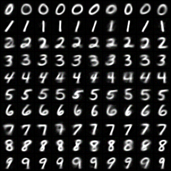
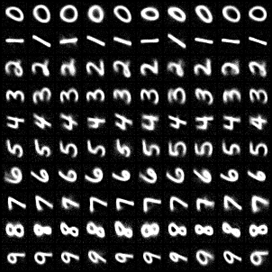
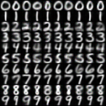
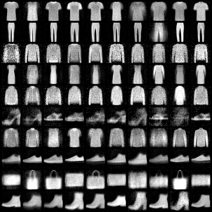
Figure 5: Condensed dataset. Top left: MNIST, top right: RMNIST, bottom left: USPS, bottom right: FMNIST.

For MNIST, RMNIST, FMNIST, and USPS we condensed the dataset using Gradient Matching Zhao et al. [2021]. The setup for creating the condensed dataset was the same architecture and the same data preprocessing as used for training. Condensation was performed in two cases: 1 per label and 10 per label. The dataset after condensation is shown in Fig. 5. In CIFAR10, we used a more sophisticated dataset condensation [Nguyen et al., 2021]. Since compressed datasets were publicly available, we use them.

B.4 Setup in Fig. 1

Can we find the effective permutation for model merging without data? To answer the question, we generated a variety of permutations and plotted the correlations between test loss on the mixed dataset and neuronal permutation criteria in Fig. 1. The datasets used were MNIST and RMNIST-90. To produce permutation variations, we used $25$ patterns of FWM $\beta$ from $0$ to $1$ and max iteration of WM search from $\left[2,5,300\right]$ and random number seed $\left[0,1,2,3,4\right]$. Of the 375 permutations generated, 30 are unique.

B.5 Setup of Tab. 2

To test the stability of the merging models method, we loaded the checkpoints of the trained model A and B and experimented with different random number seeds. We merge the models five times to show the average test accuracy. The error bars are small enough to be omitted. Also, only SPLIT-CIFAR10 does not measure error bars due to computational cost issues.

B.6 Hardware and software

Our SPLIT-CIFAR10 experiments are done on a workstation with Intel Xeon(R) Gold 6128 CPU 8 cores, 128GB RAM, and 4 NVIDIA Tesla V100 GPU. Other experiments are done on M1 max mac book pro. The deep learning models are implemented in PyTorch Paszke et al. [2019].

Appendix C Additional Experiments

C.1 Preliminary Experiments for OT Fusion

Table 3: Test accuracy on MNIST (%).

	Model A	Model B	Model AB (Naïve)	Model AB (OT)
$\lambda=0.5$, ${\rm sr}=0.1$	95.29	88.06	80.25	85.98
$\lambda=0.5$, ${\rm sr}=0$	9.82	88.21	13.06	10.1
$\lambda=0.2$, ${\rm sr}=0.1$	95.29	88.06	82.07	94.43
$\lambda=0.2$, ${\rm sr}=0$	9.82	88.21	9.82	10.1

To evaluate the OT performance in the case of complete label separation, we conducted experiments varying the hyperparameters in Fig. 2 of the OT paper [Singh and Jaggi, 2020]. In Fig. 2 of the OT paper, Model A was trained using Label 4 and $10\%$ of labels other than 4, and Model B was trained using $100\%$ of data other than Label 4. Table 3 shows the test accuracy on the MNIST data. The $\lambda$ is the coefficients of model combination, and ${\rm sr}$ is the percentage of non-specific labels used. For example, if we use $10\%$ of labels other than Label 4 and 4 for Model A, then ${\rm sr}=0.1$. Here, experiments were conducted with ${\rm sr}=0.0$ as the difficult task, rather than ${\rm sr}=0.1$ used in the paper. We also experimented with $\lambda=0.5$, which is the simple average of the model parameters, and $\lambda=0.2$, which is the best parameter in the paper. Since MNIST is a simple dataset, even with ${\rm sr}=0.1$, Model-A achieves $95\%$ accuracy, while with ${\rm sr}=0.0$, only $4$ labels are trained, which reduces the accuracy to $10\%$. For $\lambda=0.2$ and ${\rm sr}=0.1$, the accuracy of Model-AB (OT) almost reproduces the previous study values with $82\%$. When ${\rm sr}=0$, the test accuracy of Model AB (OT) is $10\%$, indicating that OT has difficulty merging models between completely separated labels. For ${\rm sr}=0.1$, Model A contains all the label information, so it is optimal to merge Model A more as $\lambda=0.2$. On the other hand, for ${\rm sr}=0$, Model A is completely independent of the label, so it is optimal to merge half of the model as $\lambda=0.5$ is considered to be the optimal case of mixing half and half as $\lambda=0.5$.

C.2 Failed Idea: Fisher Connection

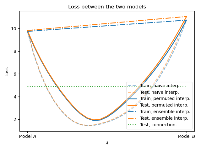
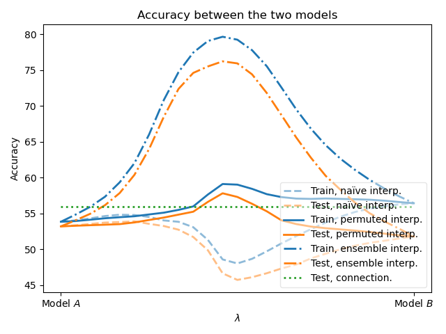
Figure 6: Fisher strategy

We show the advantage of switching from mean strategy to Fisher strategy for merging models after performing WM as Eq. (7). Figure 6 shows the loss and accuracy between MNIST and FMNIST. The green line represents the case of merging models using $\mathbf{w_{AB}}=\frac{1}{2}\left(F_{AB}\right)^{-1}\left(F_{A}\mathbf{w_{A}}+F_{B}\mathbf{w_{B}}\right)$ on $\lambda=0.5$. The Fisher strategy is less accurate than the average strategy. The Fisher strategy fails because it is numerically unstable due to the use of eigenvector directions with small eigenvalues of the Fisher information matrix around the flat solution.

C.3 Failed Idea: Flat Weight Matching

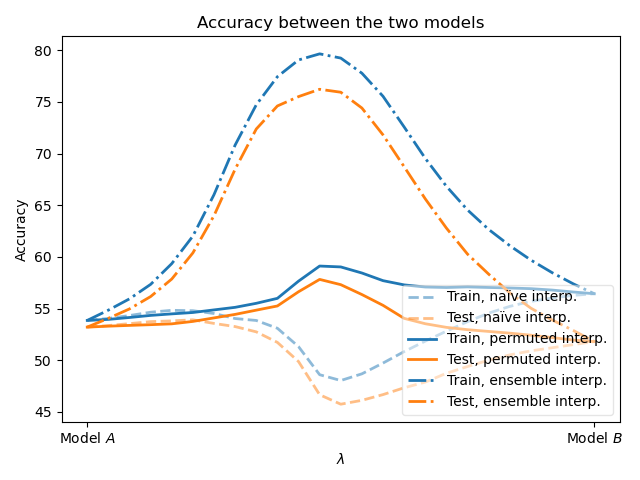
(a) WM

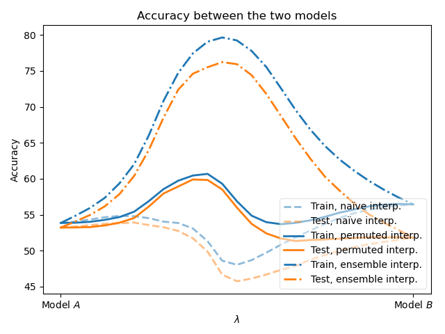
(b) FWM

Figure 7: Acc with FWM on MNIST-FMNIST

Section 3.3 shows that the flatness of the loss landscape is important for successful merging models. Thus, we propose Flat Weight Matching (FWM), which adds to the cost function of WM the regularization that not only the L2 distance is close, but also the loss landscape is flat as

$$\operatorname*{arg\,min}_{\pi}\left[\beta\left\|{\rm vec}\left(\mathbf{w_{A}}\right)-{\rm vec}\left(\pi\left(\mathbf{w_{B}}\right)\right)\right\|^{2}+\left(1-\beta\right)\left({\rm vec}\left(\mathbf{w_{A}}\right)-{\rm vec}\left(\pi\left(\mathbf{w_{B}}\right)\right)\right)\left.\frac{\partial\mathcal{L}_{B}}{\partial\mathbf{w}}\right|_{\mathbf{w}=\pi\left(\mathbf{w_{B}}\right)}\right],$$ (15)

where $\beta$ is the hyperparameter and the second term is a regularization that promotes flattening the loss landscape. The loss landscape of Model A is flat because it is optimized by SGD. Since the gradient of the permuted weight can be computed from a permutation of the pre-computed gradient, FWM has the advantage that the gradient does not need to be recomputed. In our experiments, we used $\beta=0.01$, which had the best performance among $\beta\in\left[0,1\right]$. Fig. 7 compares WM and FWM. Improvement with FWM was marginal. This is because regularization using local gradients on the optimal weights could not sufficient promote flatness as shown in Fig. 3.

C.4 Model Merging on Single Dataset

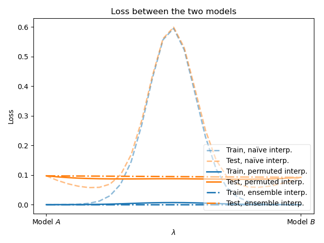
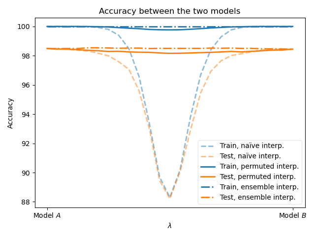
(a) MNIST

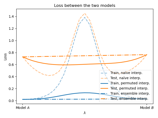
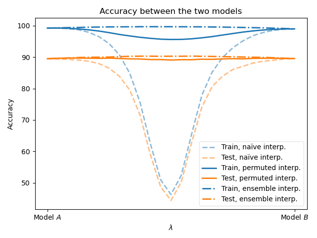
(b) FMNIST

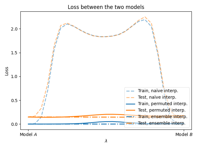
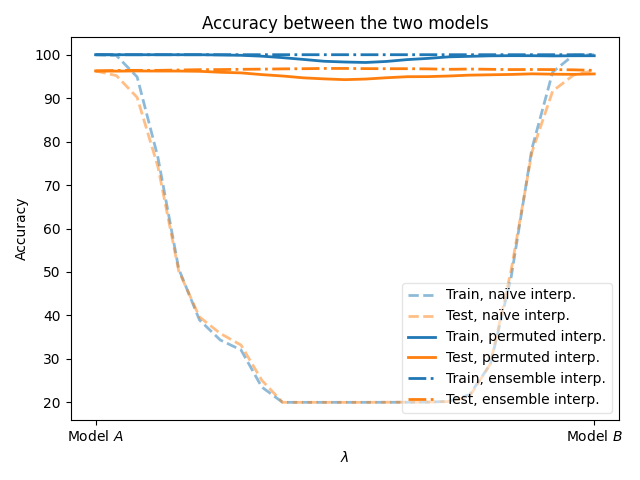
(c) SPLIT-CIFAR10-A with width multiplier 4

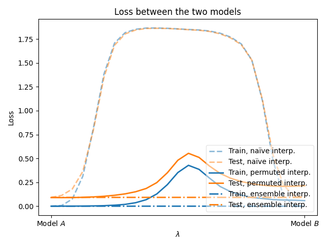
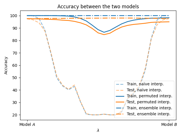
(d) SPLIT-CIFAR10-B with width multiplier 4

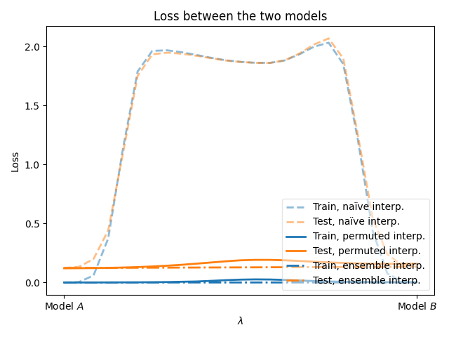
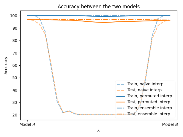
(e) SPLIT-CIFAR10-A with width multiplier 16

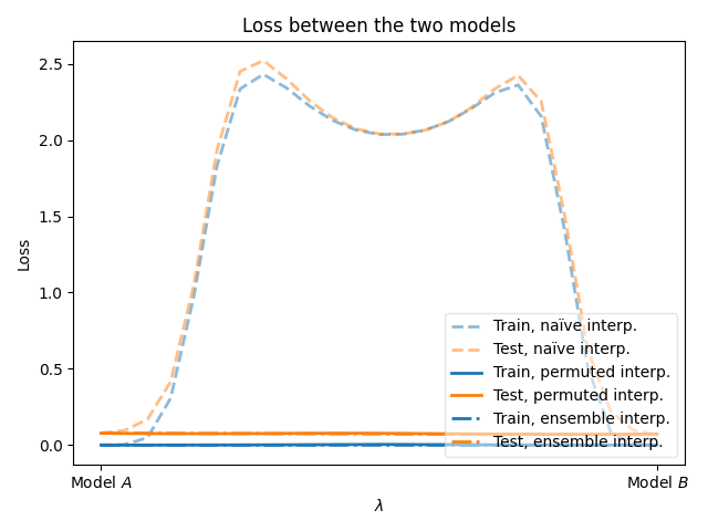
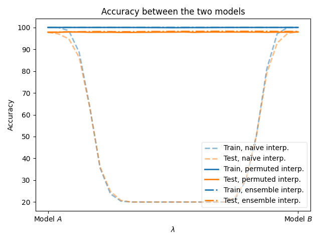
(f) SPLIT-CIFAR10-B with width multiplier 16

Figure 8: Loss and Acc of the merged model on single datasets.

This subsection presents preliminary experiments with WM merging models on a single dataset. Figure 8 shows loss and accuracy on MNIST, FMNIST, and SPLIT-CIFAR10, where SPLIT-CIFAR10 was used with ResNet20 widths of 4 and 16 times. MNIST and FMNIST successfully merge models with high accuracy in each case. SPLIT-CIFAR10 allowed for merging models with high accuracy by increasing the width by a factor of 16. For merging models between different datasets, we used merging models that can be merged on the single dataset.

C.5 Effect of Model Width

This section discusses the impact of Model Width on merging models. It is known that LMC on a single dataset is more valid the larger the Model Width is [Ainsworth et al., 2023]. Since it is difficult to synthesize models on different data if they are not synthesized well on the same dataset, the larger the Model Width on different datasets, the higher the accuracy after merging tends to be.

C.6 Overlap of Critical Weights

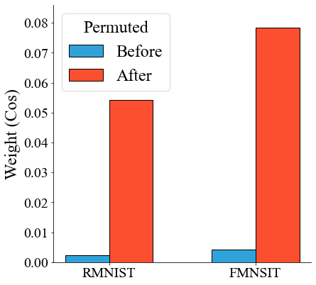
(a) Weight Vector

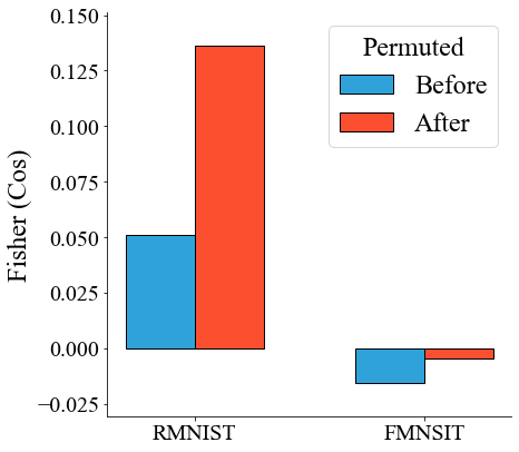
(b) Importance Vector

Figure 9: Overlap of weights and importance vector of weights between before and after permutations on MNIST-RMNIST and MNIST-FMNIST. Before and after permutation of RMNIST and FMNIST cos distance to MNIST.

To reveal the properties of weight permutations, we measure the importance vector as the diagonal components of the Fisher information matrix and evaluate the overlap between Models A and B. Existing methods for learning multiple datasets, such as continuous learning, embed knowledge of each dataset into a single network. These embeddings avoid overlapping weights that are important to the inference of each dataset [Kirkpatrick et al., 2017, Fernando et al., 2017]. In other words, different forward propagation paths are used in inference for different datasets. Our definition of the importance vector is a one-dimensional arrangement of the diagonal components of the Fisher information matrix on mixed datasets, as in Kirkpatrick et al. [2017]. The overlap of importance vectors is defined by the cos distance between the importance vectors of Models A and B. Figure 9 shows the results in MNIST-RMNIST and MNIST-FMNIST by using STE. They are the case of model merging with and without shared labels. The permutation for model merging shows that the overlap in the importance of the weights is not reduced. This is a different result from existing studies and does not indicate that different forward propagation path are used for different datasets. Furthermore, Fig. 9 shows the cos distance of the weights between Models A and B before and after the permutation. The permutation by STE also increased the cos distance of the weights as in the case of WM. This indicates that STE also reduces the L2 distance of weights between models.

References

- Ainsworth et al. [2023] Samuel Ainsworth, Jonathan Hayase, and Siddhartha Srinivasa. Git re-basin: Merging models modulo permutation symmetries. In The Eleventh International Conference on Learning Representations, 2023. URL https://openreview.net/forum?id=CQsmMYmlP5T.
- Akhlaghi and Sukhov [2018] Milad I. Akhlaghi and Sergey V. Sukhov. Knowledge fusion in feedforward artificial neural networks. Neural Processing Letters, 48(1):257–272, 2018. doi: 10.1007/s11063-017-9712-5. URL https://doi.org/10.1007/s11063-017-9712-5.
-
AUTOMATIC1111 [2022]
AUTOMATIC1111.
Stable diffusion web ui.
https://github.com/AUTOMATIC1111/stable-diffusion-webui, 2022. Accessed: May 8, 2023. - Breiman [1996] Leo Breiman. Bagging predictors. Machine learning, 24:123–140, 1996.
- Entezari et al. [2021] Rahim Entezari, Hanie Sedghi, Olga Saukh, and Behnam Neyshabur. The role of permutation invariance in linear mode connectivity of neural networks. arXiv preprint arXiv:2110.06296, 2021.
- Fernando et al. [2017] Chrisantha Fernando, Dylan Banarse, Charles Blundell, Yori Zwols, David Ha, Andrei A Rusu, Alexander Pritzel, and Daan Wierstra. Pathnet: Evolution channels gradient descent in super neural networks. arXiv preprint arXiv:1701.08734, 2017.
- Frankle and Carbin [2019] Jonathan Frankle and Michael Carbin. The lottery ticket hypothesis: Finding sparse, trainable neural networks. In International Conference on Learning Representations, 2019. URL https://openreview.net/forum?id=rJl-b3RcF7.
- Frankle et al. [2020] Jonathan Frankle, Gintare Karolina Dziugaite, Daniel Roy, and Michael Carbin. Linear mode connectivity and the lottery ticket hypothesis. In International Conference on Machine Learning, pages 3259–3269. PMLR, 2020.
- Garipov et al. [2018] Timur Garipov, Pavel Izmailov, Dmitrii Podoprikhin, Dmitry P Vetrov, and Andrew G Wilson. Loss surfaces, mode connectivity, and fast ensembling of dnns. Advances in neural information processing systems, 31, 2018.
- He et al. [2018] Xiaoxi He, Zimu Zhou, and Lothar Thiele. Multi-task zipping via layer-wise neuron sharing. Advances in Neural Information Processing Systems, 31, 2018.
- Hull [1994] Jonathan J. Hull. A database for handwritten text recognition research. IEEE Transactions on pattern analysis and machine intelligence, 16(5):550–554, 1994.
- Jordan et al. [2022] Keller Jordan, Hanie Sedghi, Olga Saukh, Rahim Entezari, and Behnam Neyshabur. Repair: Renormalizing permuted activations for interpolation repair. arXiv preprint arXiv:2211.08403, 2022.
- Kirkpatrick et al. [2017] James Kirkpatrick, Razvan Pascanu, Neil Rabinowitz, Joel Veness, Guillaume Desjardins, Andrei A Rusu, Kieran Milan, John Quan, Tiago Ramalho, Agnieszka Grabska-Barwinska, et al. Overcoming catastrophic forgetting in neural networks. Proceedings of the national academy of sciences, 114(13):3521–3526, 2017.
- Krizhevsky et al. [2009] Alex Krizhevsky, Geoffrey Hinton, et al. Learning multiple layers of features from tiny images. 2009.
- LeCun et al. [1998] Yann LeCun, Léon Bottou, Yoshua Bengio, and Patrick Haffner. Gradient-based learning applied to document recognition. Proceedings of the IEEE, 86(11):2278–2324, 1998.
- Leontev et al. [2020] Mikhail Iu Leontev, Viktoriia Islenteva, and Sergey V Sukhov. Non-iterative knowledge fusion in deep convolutional neural networks. Neural Processing Letters, 51(1):1–22, 2020.
- Li et al. [2022] Margaret Li, Suchin Gururangan, Tim Dettmers, Mike Lewis, Tim Althoff, Noah A Smith, and Luke Zettlemoyer. Branch-train-merge: Embarrassingly parallel training of expert language models. arXiv preprint arXiv:2208.03306, 2022.
- Mallya and Lazebnik [2018] Arun Mallya and Svetlana Lazebnik. Packnet: Adding multiple tasks to a single network by iterative pruning. In Proceedings of the IEEE conference on Computer Vision and Pattern Recognition, pages 7765–7773, 2018.
- McMahan et al. [2017] Brendan McMahan, Eider Moore, Daniel Ramage, Seth Hampson, and Blaise Aguera y Arcas. Communication-efficient learning of deep networks from decentralized data. In Artificial intelligence and statistics, pages 1273–1282. PMLR, 2017.
- Neyshabur et al. [2020] Behnam Neyshabur, Hanie Sedghi, and Chiyuan Zhang. What is being transferred in transfer learning? In H. Larochelle, M. Ranzato, R. Hadsell, M.F. Balcan, and H. Lin, editors, Advances in Neural Information Processing Systems, volume 33, pages 512–523, 2020.
- Nguyen et al. [2021] Timothy Nguyen, Roman Novak, Lechao Xiao, and Jaehoon Lee. Dataset distillation with infinitely wide convolutional networks. Advances in Neural Information Processing Systems, 34:5186–5198, 2021.
- Paszke et al. [2019] Adam Paszke, Sam Gross, Francisco Massa, Adam Lerer, James Bradbury, Gregory Chanan, Trevor Killeen, Zeming Lin, Natalia Gimelshein, Luca Antiga, Alban Desmaison, Andreas Kopf, Edward Yang, Zachary DeVito, Martin Raison, Alykhan Tejani, Sasank Chilamkurthy, Benoit Steiner, Lu Fang, Junjie Bai, and Soumith Chintala. Pytorch: An imperative style, high-performance deep learning library. In H. Wallach, H. Larochelle, A. Beygelzimer, F. d'Alché-Buc, E. Fox, and R. Garnett, editors, Advances in Neural Information Processing Systems 32, pages 8024–8035. Curran Associates, Inc., 2019. URL http://papers.neurips.cc/paper/9015-pytorch-an-imperative-style-high-performance-deep-learning-library.pdf.
- Schapire [1999] Robert E Schapire. A brief introduction to boosting. In International Joint Conference on Artificial Intelligence, volume 99, pages 1401–1406. Citeseer, 1999.
- Silver et al. [2013] Daniel L Silver, Qiang Yang, and Lianghao Li. Lifelong machine learning systems: Beyond learning algorithms. In 2013 Association for the Advancement of Artificial Intelligence spring symposium series, 2013.
- Singh and Jaggi [2020] Sidak Pal Singh and Martin Jaggi. Model fusion via optimal transport. Advances in Neural Information Processing Systems, 33:22045–22055, 2020.
- Wolpert [1992] David H Wolpert. Stacked generalization. Neural networks, 5(2):241–259, 1992.
- Xiao et al. [2017] Han Xiao, Kashif Rasul, and Roland Vollgraf. Fashion-mnist: a novel image dataset for benchmarking machine learning algorithms, 2017.
- Zhao et al. [2021] Bo Zhao, Konda Reddy Mopuri, and Hakan Bilen. Dataset condensation with gradient matching. In International Conference on Learning Representations, 2021. URL https://openreview.net/forum?id=mSAKhLYLSsl.