Kinematics and flux evolution of superluminal components in QSO B1308+326

Abstract

Context. Search for Doppler-boosting effect in flux evolution of superluminal components in blazars has been an important subject, which can help to clarify their kinematic and emission properties.

Aims. The kinematics and flux evolution observed at 15 GHz for the three superluminal components (knot-c, -i and -k) in QSO B1308+326 (z=0.997) were investigated in detail.

Methods. It is shown that the precessing jet nozzle model previously proposed by Qian et al. (1991, 2014, 2017, 2022a, 2022b) can be used to fully simulate their kinematics on pc-scales with a nozzle precession period of 16.9 yr.

Results. With the acceleration/deceleration in their motion found in the model-simulation of their kinematics we can derive their bulk Lorentz factor and Doppler factor as function of time and predict their Doppler-boosting effect.

Conclusions. Interstingly, the flux evolution of the three superluminal components can be well intrepreted in terms of their Doppler-boosting effect. The full explanation of both their kinematic behavior and flux evolution validates our precessing nozzle model and confirms that superluminal components are physical entities moving relativistically toward us at small viewing angles.

1 Introduction

B1308+326 is a high redshift quasar (z=0.997). In historical records it was observed as being optically variable with a long-term variability amplitude of $M_{B}\sim$5.6 mag and highly polarization and was classified as one of the most variable BL Lac objects (Angel & Stockman An80 (1980)). It is a $\gamma$-ray source detected by the ”Fermi Gamma-ray Observatory” (Ackermann et al. Ack11 (2011), Acero et al. Ac15 (2015)). So B1308+326 radiates across the entire electromagnetic spectrum from radio-mm-NIR-optical through X-ray to $\gamma$-ray bands. Very strong variability has been observed in all these wavebands with various timescales (hours/days to years).
B1308+326 is a low-synchrotron-peaked high polarization quasar, showing a radio core-jet structure on pc-scales with superluminal components ejected from its core. In the previous works (Qian et al. Qi17 (2017), Britzen et al. Br17 (2017)) the kinematic behaviors of the five superlumianl components (knot-c, -h, -i, -j and -k) observed at 15 GHz in B1308+326 were well model-simulated in terms of our precessing nozzle scenario with a precession period of 16.9$\pm$0.85 years, revealing their motion along the precessing common trajectory in the innermost jet regions corresponding to their precession phases.
The interesting results (including the modeled distribution of the precessing common trajectories, the model-fits of the observed trajectories, the periodic swing of their ejection position angle and the relation between the position angle and their initial viewing angle) are re-plotted in Figures 1 and 2. Although these results are ”very nice !!” as an anonymous referee commented, they are not consummate, because the bulk Lorentz factor and Doppler factor derived for the superluminal knots in our model-simulations were not further investigated to find out the association of their flux evolution with the Doppler-boosting effect. Therefore, one would ask the questions: What about the flux-density evolution of the superluminal knots ? Would the evolving line-of-sight of the feature trajectories and their bulk Lorentz factor produce measurable changes in the flux densities? Would the used precession model be able to predict (at least part of) the light curves of the different componnets ?
In this paper we shall discuss the flux evolution combined with the model-fitting of the kinematic behavior for three superluminal components (knot-c, -i and -k), demonstrating that their Doppler-boosting effect plays an important role for understanding their kinematic, dynamic and emission properties. That is, the inclusion of flux evolution can help to accurately interpret their VLBI-kinematics, correctly deriving their bulk Lorentz factor and Doppler factor as function of time in the model-simulations and showing that their flux evolution can be well explained in terms of the Doppler-boosting effect.

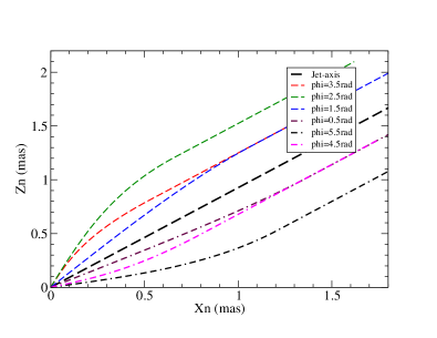
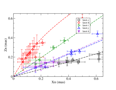
Figure 1: Left panel: the distribution of precessing common trajectories modeled for superluminal components in B1308+326 at precession phases $\phi$=0.5, 1.5, 2.5, 3.5, 4.5 and 5.5 rad. Right panel: model fits of the trajectories for knot-c, -h, -i, -j and -k in the innermost jet regions. Within $X_{n}$$\sim$0.3–0.5 mas all the trajectories can be well fitted in terms of the precessing common trajectory pattern.

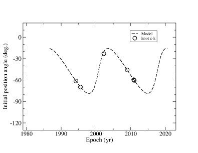
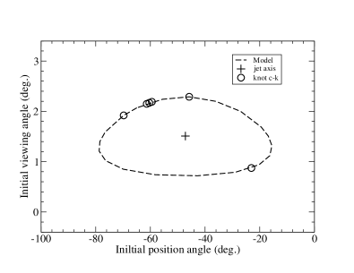
Figure 2: Left panel: the periodic swing of ejection position angle PA(t) produced by the precession of the jet-nozzle for knot-c, -d, -h, -i, -j and -k. Right panel: relation $\theta(PA)$ between the ejection position angle and the viewing angle for these components.

2 Recapitulation of the precessing nozzle scenario

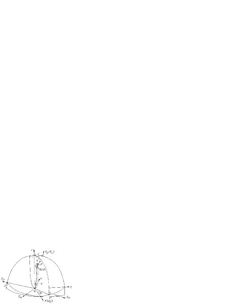
Figure 3: Geometry of the precession nozzle model (not to scale), adopted from Qian (Qi17 (2017)). Parameters $\epsilon$ and $\psi$ define the (X,Z)-plane relative to the coordinate system ($X_{n},Y_{n},Z_{n}$) with Z-axis taken as the axis of precession. The $Y_{p}$ axis indicates the direction toward the observer; the position of a superluminal component is defined by parameters (A, $\Phi$): $A(Z)$ is the amplitude function and $\Phi$ is the azimuthal angle (or phase); the plane ($X_{p}$,$Z_{p}$) represents the plane of the sky; $\theta$ denotes the angle between the knot’s velocity vector (${\bf{S}}$) and the direction toward the observer (${\bf{V}}$). $\eta$ is the initial half opening angle of the precessing jet cone.

In order to perform the model-fitting of the kinematics of B1308+326 we will use the precessing nozzle scenario previously proposed in Qian et al. (Qi17 (2017)). Firstly, we recapitulate the formalism of the model. The geometry of this model is shown in Figure 3, where three coordinate systems are used.
The coordinate system (${X_{p}},{Y_{p}},{Z_{p}}$) has the $Y_{p}$-axis directed toward the observer, i.e. the plane ($X_{p}$, $Z_{p}$) is defined as the sky plane. In this plane the $Z_{n}$-axis is defined as the direction toward the north pole and the $X_{n}$-axis as opposite to the direction of right ascension. The observed position angle of VLBI knots is measured in clockwise from the $Z_{n}$-axis. We define a third coordinate system $(X,Y,Z)$: the $X$-axis coincides with the axis $X_{p}$ and the $Z$-axis is situated in the $Y_{p}$-$Z_{p}$ plane forming an angle $\epsilon$ with the $Y_{p}$-axis. The $Z$-axis is defined as the jet-axis around which the precessing nozzle rotates. $\psi$ denotes the angle between the $X(X_{p})$-axis and the $X_{n}$-axis. The precession cone has an initial half opening angle of $\eta$.
We assume that the superluminal knots move along curved trajectories (as shown in Figure 3), defined by the amplitude function A(Z) and phase $\Phi$, which changes successively due to the nozzle precession. In Figure 3, ${\bf{S}}$ denotes the direction of the spatial velocity and ${\bf{V}}$ denotes the direction toward the observer (parallel to the direction $Y_{p}$). $\theta$ denotes the viewing angle of the knot’s motion.
Thus, the trajectory of a knot can be described in the $(X,Y,Z)$ system as follows.

$$X({Z},\Phi)=A({Z}){\cos{\Phi}},$$ (1)

$$Y({Z},\Phi)=A({Z}){\sin\Phi}.$$ (2)

The projection of the spatial trajectory on the sky plane is defined by

$${X_{n}({Z},{\Phi})}={X_{p}({Z,\Phi})}{\cos{\psi}}-{Z_{p}({Z,\Phi})}{\sin{\psi}},$$ (3)

$${Z_{n}({Z},{\Phi})}={X_{p}({Z,\Phi})}{\sin{\psi}}+{Z_{p}({Z,\Phi})}{\cos{\psi}},$$ (4)

where $\psi$ is the angle between the $X(X_{p})$-axis and the $X_{n}$-axis,

$${X_{p}(Z,\Phi)}=X(Z,\Phi),$$ (5)

$${Z_{p}(Z,\Phi)}={Z}{\sin{\epsilon}}-{Y({Z},\Phi)}{\cos{\epsilon}}.$$ (6)

We give the formulas for calculating the viewing angle $\theta$, Doppler factor $\delta$, apparent transverse velocity $v_{app}$ and elapsed time $T$ after ejection as follows.

• Viewing angle $\theta$

  $${\theta}=\arccos[\cos{\Delta}(\cos{\epsilon}+\sin{\epsilon}\tan{{\Delta}_{p}})].$$ (7)

  Where

  $${\Delta}=\arctan\left[\left(\frac{dX}{dZ}\right)^{2}+\left(\frac{dY}{dZ}\right)^{2}\right]^{1/2},$$ (8)

  $\Delta$ is the angle between the spatial velocity vector and the $Z$-axis, and

  $${{\Delta}_{p}}=\arctan\left(\frac{dY}{dZ}\right)$$ (9)

  is the projection of $\Delta$ on the $(Y,Z)$-plane.

• Apparent transverse velocity $v_{app}$ and Doppler factor $\delta$

  $${v_{app}}=c{{\beta}_{app}}={\frac{c{\beta}{\sin{\theta}}}{1-{\beta}{\cos{\theta}}}},$$ (10)

  and

  $${\delta}={\frac{1}{{\Gamma}(1-{\beta}{\cos{\theta}})}},$$ (11)

  where $\beta$=$\frac{v}{c}$, $v$ is the spatial velocity of the knot and $\Gamma$=$(1-{\beta}^{2})^{-1/2}$ is the bulk Lorentz factor.

• Elapsed time $T$, at which the knot reaches the axial distance $Z$:

  $${T}={\int_{0}^{Z}}{\frac{1+z}{{\Gamma}{\delta}{v}{\cos{{\Delta}_{s}}}}}{d{Z}},$$ (12)

  where $z$ is the redshift of B1308+326,

  $${\Delta}_{s}=\arccos\left[\left(\frac{dX}{dZ}\right)^{2}+\left(\frac{dY}{dZ}\right)^{2}+1\right]^{-1/2},$$ (13)

  where ${\Delta}_{s}$ is the instantaneous angle between the velocity vector and the $Z$-axis.

All coordinates and the amplitude $A(Z)$ are measured in units of milliarcsecond (mas). $\theta$ and v are instantaneous quantities at an elapsed time $T$.

2.1 Precessing common trajectory pattern

As defined above, each of the superluminal components moves along a curved (collimated) track described by the amplitude function A(Z) and a constant phase $\Phi$, while for the successive knots the phase changes due to precession. That is, the superluminal components move along the precessing common trajectory. We choose the following pattern for describing the precessing common trajectory.
Its amplitude $A(Z)$ is taken as a function of $Z$:
when $Z$${\leq}b$,

$${A(Z)}={A_{0}}{\frac{2b}{\pi}}{\sin\left(\frac{{\pi}{Z}}{2b}\right)},$$ (14)

and when $Z>b$,

$${A(Z)}={A_{0}}{\frac{2b}{\pi}}.$$ (15)

Parameter $b$ may be regarded as a ’collimation parameter’ to describe the shape of the jet collimation. The phase $\Phi$ is defined by parameter $\phi$ for a specific trajectory:

$${\Phi}={\phi}+{{\Phi}_{0}},$$ (16)

${\Phi}_{0}$ is an arbitrary constant and $\phi$ is defined as the precessing phase.

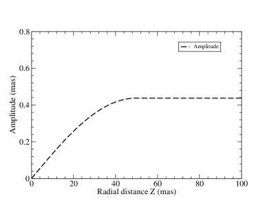
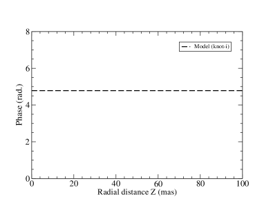
Figure 4: The assumed amplitude function $A(Z)$ and phase $\Phi$ for describing the trajectory of a knot. Here $\Phi$=$\Phi_{0}$+$\phi$=4.783 rad, corresponding to the precession phase $\phi$=1.0 rad and ${\Phi}_{0}$=3.783 rad. See text.

Since ${\frac{d\Phi}{dZ}}$=0, we have

$${\frac{dX}{dZ}}={\frac{dA}{dZ}}{\cos{\Phi}},$$ (17)

$${\frac{dY}{dZ}}={\frac{dA}{dZ}}{\sin{\Phi}}.$$ (18)

Thus, from Eqs. (8), (9) and (13) we have

$${\Delta}={\arctan\left(\frac{dA}{dZ}\right)},$$ (19)

$${{\Delta}_{p}}={\arctan\left(\frac{dA}{dZ}\sin{\Phi}\right)},$$ (20)

$${{{\Delta}_{s}}}=\arccos\left[\left(1+\left(\frac{dA}{dZ}\right)^{2}\right)^{-1/2}\right].$$ (21)

Substituting $\Delta$, ${\Delta}_{p}$ and ${\Delta}_{s}$ into Eqs. (7) and (10)–(12), we can calculate the viewing angle $\theta$, apparent velocity ${\beta}_{app}$, Doppler factor $\delta$ and elapsed time $T$.
We should point out that the assumed pattern of the precessing common trajectory (see Figure 4 below) closely represents the field structure configurations observed in the jets of radio galaxies and blazars. For example, the giant radio galaxy M87 which has a powerful optical-radio jet and a supermassive black hole of $\sim$6$\times$$10^{9}{M_{\odot}}$, is the best possible target for studying the initial jet formation/collimation process (Biretta et al. Bi02 (2002)). Nakamura & Asada (Na13 (2013)) (also, Asada & Nakamura As12 (2012); Doeleman et al. Do12 (2012)) have found that its innermost jet emission components follow an extrapolated parabolic streamline, so that the jet has a single power-law structure with a nearly five orders of magnitude in the distance starting from the vicinity of the supermassive black hole, less than ten Schwarzschild radii. They have also proposed a magnetohydrodynamic nozzle model to interpret the property of the bulk jet acceleration and assumed that the MHD nozzle consists of a hollow parabolic tube. Most recently, Lu et al. (Lu23 (2023)) (also cf. Kim et al. Kim23 (2023)) present the parabolic jet profile extending to the jet-axis distance of $\sim$70$\mu$as (or $\sim$10$R_{s}$, $R_{s}$ – Schwarzschild radius).
Moreover, general relativistic MHD simulations (e.g., McKinney et al. Mc12 (2012)) reveal that the magnetic field structures (or configurations) near the horizon of a rotating black hole closely correspond to a parabolic configuration which is consistent with the analytic results given by Beskin & Zheltoukhov (Bes13 (2013)) for a field geometry: a radial field near the horizon and a vertical field far from the black hole. In these configurations, the distribution of the magnetic field and the field angular velocity profile near the horizon can be described in detail (Punsly Pu01 (2001); McKinney et al. Mc12 (2012); Beskin & Zheltoukhov Bes13 (2013)). In addition, the assumed pattern is also quite similar to the fork-structure observed in the prominent blazar OJ287 by Tateyama (Ta13 (2013)).
In fact, in the previous works we have already adopted such a kind of common precessing trajectory pattern to study the kinematics of the superluminal components in a few blazars, e.g., 3C279 (Qian et al. Qi19 (2019); Qian Qi12 (2012), Qi13 (2013),), 3C454.3 (Qian et al. Qi14 (2014), Qi21 (2021)), OJ287 (Qian 2018b ), 3C345 (Qian et al. Qi91 (1991), Qian 2022a , 2022b ), and also in the QSOs PG1302-132 (Qian et al. 2018a ) and NRAO 150 (Qian Qi16 (2016)).
In this paper we will adopt the concordant cosmology model with ${\Omega}_{\Lambda}$=0.73, ${\Omega}_{m}$=0.27 and Hubble constant $H_{0}$=71 km ${{\rm{s}}^{-1}}$ ${{\rm{Mpc}}^{-1}}$ (Spergel et al. Sp03 (2003)). For the redshift z=0.997 of B1308+326, we have its luminosity distance $D_{L}$=6.61 Gpc and the angular diameter distance $D_{A}$=1.66 Gpc (Hogg Ho99 (1999); Pen Pe99 (1999)). The angular scale is 1 mas=8.04 pc and the proper motion of 1 mas/yr is equivalent to an apparent velocity of 52.34c.

3 Selection of model parameters

In our precessing jet nozzle model, the jet nozzle precesses around a fixed jet axis and the knots are ejected from the nozzle, moving along their individual trajectories (of a common pattern, ballistic or helical, Qian Qi16 (2016)) with different bulk Lorentz factors. The precession of the nozzle leads to the rotation of the ejection direction of the knots or the periodic position angle swing. The combination of a sequence of isolated knots (and associated magnetized plasma flows) ejected from this nozzle will construct the structure of the whole jet and its evolution seen on VLBI-maps (e.g., Tateyama & Kingham Ta04 (2004); Qian et al. Qi17 (2017); Tateyama Ta09 (2009), Ta13 (2013); Qian Qi14 (2014)).
In order to model-fit the kinematics of the superluminal knots in terms of our precessing jet-nozzle model, the model parameters, defining the jet-axis direction ($\epsilon$, $\psi$), the pattern of the precessing common track ($A_{0}$, b), precession period $T_{p}$ and phase ($\Phi_{0}$, $\phi$) should be approriately selected. We shall adopt the same values as used in the previous work (Qian et al. Qi17 (2017)) as follows:

$\epsilon$ = $1.5^{\circ}$
$\psi$ = –$42.8^{\circ}$
$A_{0}$ = 1.375$\times{10^{-2}}$ mas
$b$ = 50 mas
${\Phi}_{0}$ = 3.783 rad
$T_{p}$ = 16.9 yr

The ejection epoch $t_{0}$ for the knots can be calculated from their precession phase $\phi$:

$${t_{0}}=1995.54+{\frac{T_{p}}{2\pi}}(6.0-{\phi}).$$ (22)

The kinematic parameters including the bulk Lorentz factor, viewing angle, apparent velocity and Doppler factor as function of time will be derived through the model-fitting process.
In order to model-fit the light curves of the superluminal knots the observed flux density ${S_{obs}}(\nu,t)$ can be calculated as:

$${{S_{obs}}(\nu,t)}={{S_{int}}(\nu,t)}{[\delta(t)]^{3+\alpha(\nu,t)}}$$ (23)

${S_{int}}(\nu,t)$ – intrinsic flux density; $\delta(t)$ – Doppler factor; $\alpha(\nu,t)$ – spectral index ($S_{\nu}$ $\propto$ ${\nu^{-\alpha}}$). In most cases ${S_{int}}(\nu,t)$=${S_{int}}(\nu)$ and $\alpha(\nu,t)$=$\alpha(\nu)$ are assumed.

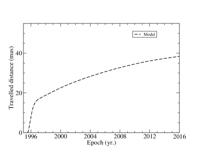
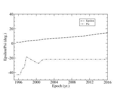
Figure 5: Knot-c: Model fitting of the entire kinematics (1995–2014). Left panel: the modeled traveled distance Z(t) along the Z-axis. Right panel: the modeled curves for parameters $\epsilon(t)$ and $\psi(t)$. After 1996.40 $\psi$ increased quickly, implying a rotation of the (X,Z)-plane relative to the coordinate system ($X_{n},Y_{n},Z_{n}$) and knot-c started to move along its own individual track.

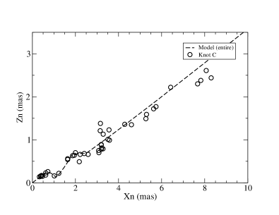
Figure 6: Knot-c: the model fit of the entire trajectory extending to core distance $r_{n}$$\sim$8.5 mas (during 1996–2014). The curvature within $X_{n}{\sim}$1.7 mas is well fitted.

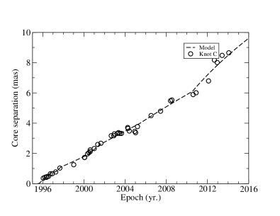
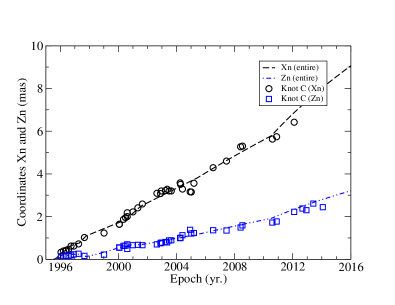
Figure 7: Knot-c: Model fitting of the entire kinematics (1995–2014). Left panel: the model-fit of the core separation $r_{n}(t)$. Right panel: the model-fits of coordinates $X_{n}(t)$ and $Z_{n}(t)$. All the kinematic features are well fitted in terms of the precessing nozzle model extending to core distance $r_{n}{\sim}$8.5 mas (during 1996–2014).

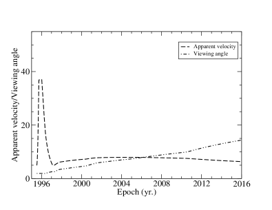
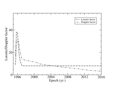
Figure 8: Knot-c: Model fitting of the entire kinematics (1995–2014). Left panel: the model-derived apparent velocity $\beta_{app}(t)$ and viewing angle $\theta(t)$. Right panel: the model-derived bulk Lorentz factor $\Gamma(t)$ and Doppler factor $\delta(t)$. The prominent feature is $\delta(t)$$<$$\Gamma(t)$ during the peaking stage.

4 Knot-c: Model-fitting results

The model fitting results for knot-c will be presented in two parts: (1) for entire kinematics (1995–2014) in Fig.5–8 and (2) for the inner jet region (1995–2001.5, $r_{n}{\leq}2.5$ mas) in Fig.9-13.

4.1 Knot-c: model-fitting of entire kinematics (1995-2014)

Its ejection epoch $t_{0}$=1995.54, corresponding to a precession phase $\phi$=6.0 rad.
In Fig.5 the traveled distance Z(t) along Z-axis (left panel) and the parameters $\epsilon(t)$ and $\psi(t)$ (right panel) are presented. During the time-interval $\sim$1996–2000 parameter $\psi$ changed quickly, implying a rotation of the XY-plane relative to the coordinate system ($X_{n},Z_{n}$).
The model-fits of the entire trajectory $Z_{n}(X_{n})$, core separation $r_{n}(t)$, coordinates $X_{n}(t)$ and $Z_{n}(t)$ are shown in Fig.6 and Fig.7, respectively. Within $r_{n}(t)\sim$8.6 mas (or till 2014.09) all these kinematic features were well fitted.
The model-derived apparent velocity $\beta_{app}(t)$ and viewing angle $\theta(t)$ (left panel) and bulk Lorentz factor $\Gamma(t)$ and Doppler factor $\delta(t)$ (right panel) are presented in Fig.8. Both show a peak structure during $\sim$1995.5–1997.0, coincident with the radio burst (see Fig.13, below).

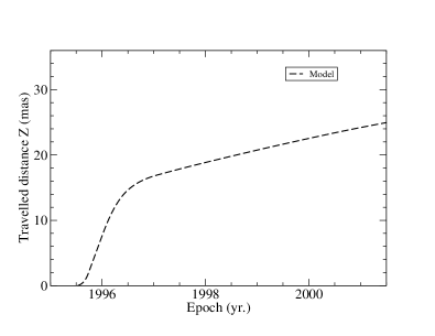
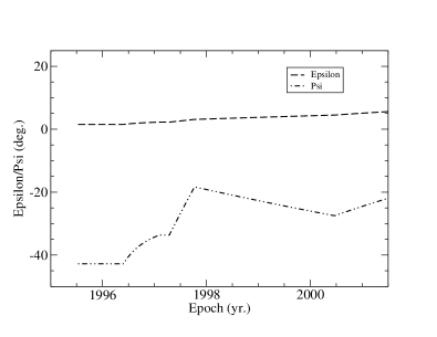
Figure 9: Knot-c: model fitting of the inner kinematics (1995.5–2001.5). Left panel: the modeled traveled distance Z(t) along the Z-axis. Right panel: the modeled curves for parameters $\epsilon(t)$ and $\psi(t)$. Within core separation $r_{n}\simeq$0.46 mas (or before 1996.40, corresponding to traveled distance Z$\leq$13.8 mas=106 pc) $\epsilon$=$1.5^{\circ}$ and $\psi$=–$42.8^{\circ}$, knot-c moved along the precessing common trajectory. Beyond $r_{n}$=0.46 mas, parameter $\psi$ increased quickly and knot-c started to move along its own individual track.

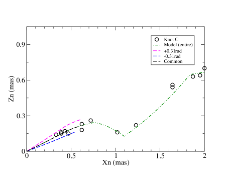
Figure 10: Knot-c: Model fitting of the inner trajectory ($X_{n}{\leq}$2 mas, 1995.5–2001.5). Within core separation $r_{n}$=0.46 mas (or coordinate $X_{n}{\leq}$0.43 mas) knot-c moved along the precessing common trajectory. Beyond that knot-c started to move along its own individual trajectory. The red and green curves are calculated for the precession phases $\phi{\pm}$0.31 rad ($\phi$=6.0 rad), demonstrating that the observational data-points are within the area confined by the two curves and showing that the precession period was derived correctly with an uncertainty of ${\sim}\pm$5% of the precession period.

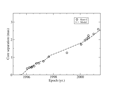
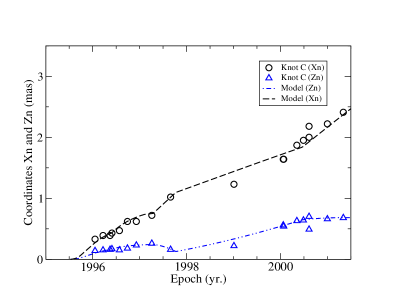
Figure 11: Knot-c: Model fitting of the kinematics (1995.5–2001.5). Left Panel: the model fit of the core separation $r_{n}(t)$. Right panel: the model fits of coordinates $X_{n}(t)$ and $Z_{n}(t)$. All the kinematic features are well fitted extending to $r_{n}{\sim}$ 2.5 mas. Before 1996.40 knot-c moved along the precessing common traejctory, while after that it started to move along its own individual track.

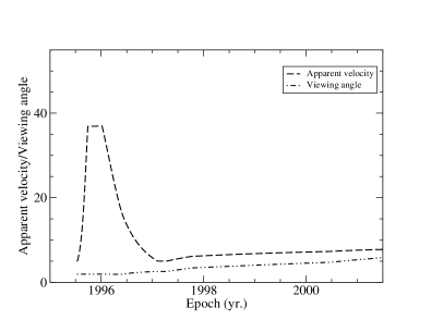
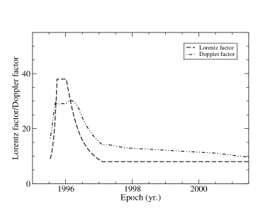
Figure 12: Knot-c: model fitting of the inner kinematics (1995.5–2001.5). Left panel: the model-derived apparent velocity $\beta_{app}(t)$ and viewing angle $\theta(t)$. Right panel: the model-derived bulk Lorentz factor $\Gamma(t)$ and Doppler factor $\delta(t)$. At 1996.15 $\delta$=$\delta_{max}$=30.2, $\Gamma$=29.7, $\beta$=29.6, while at 1996.02 $\Gamma$=$\Gamma_{max}$=38.0 and $\beta_{app}$=$\beta_{a,max}$=37.0. $\theta(t)$ varied in the range of [$1.92^{\circ}$, $5.32^{\circ}$] during 1995.5–2001.0. It is worthy of note that both $\Gamma(t)$ and $\delta(t)$ have a bump structure and during the peaking stage $\delta(t)$$<$$\Gamma(t)$.

4.2 Knot-c: Model-fitting of inner kinematics (1995.5-2001.5)

In order to investigate the flux evolution associated with its Doppler-boosting effect, the results of detailed studies on its kinematics in the inner jet regions (1995.5-2001.5) are presented in Figs.9–13.
The traveled distance Z(t) of knot-c along the jet-axis is shown in Fig.9 (left panel). The curves of parameters $\epsilon(t)$ and $\psi(t)$ are presented in the right panel. Before 1996.40 (Z$\leq$13.8 mas=106 pc) $\epsilon$=$1.5^{\circ}$ and $\psi$=–$42.8^{\circ}$ knot-c moved along the precessing common trajectory. After 1996.40 parameter $\psi$ quickly increased to $\sim$–$20^{\circ}$ and knot-c started to move along its own individual trajectory, deviating from the precessing common track. Such kind of transition from the common track pattern to the individual paths could involve some complex physical conditions (e.g., evolution of the kinetic and magnetic energy of the jet associated with the change in its current distribution, interaction between the jet and its surrounding environments, hydrodynamic and magnetohydrodynamic instabilities (e.g., Hardee Hard87 (1987), Har11 (2011); Falke et al. Fa96 (1996), Nakakura & Meier Na04 (2004), etc.).
The model-fit of the trajectory $Z_{n}(X_{n})$ during 1995.5–2001.5 is shown in Figure 10. Within coordinate $X_{n}$$\sim$0.46 mas knot-c moved along the precessing common trajectory and beyond that knot-c started to move along its own individual track, deviating from the precessing common trajectory. In the figure the red and green curves are calculated for precession phases $\phi{\pm}$0.31 rad ($\phi$=6.0 rad for ejection at 1995.54), indicating that the observational data-points are within the range defined by the two curves and the precession period is determined with an uncertainty of $\sim$$\pm$5% of the precession period (or $\sim$$\pm$0.85 yr.).
The model-fits of core separation $r_{n}(t)$ (left panel), coordinates $X_{n}(t)$ and $Z_{n}(t)$ are shown in Figure 11. Within $r_{n}{\sim}$0.46 mas knot-c moved along the precessing common trajectory and beyond that it started to move along its own individual track, deviatitng from the common track. $r_{n}(t)$, $X_{n}(t)$ and $Z_{n}(t)$ are all well fitted during 1995.5–2001.5 (in the range of $r_{n}$ extending to 2.5 mas).
The model-derived apparent velocity ${\beta_{app}}(t)$, viewing angle $\theta(t)$, bulk Lorentz factor $\Gamma(t)$ and Doppler factor $\delta(t)$ are shown in Figure 12. ${\beta_{app}}(t)$, $\Gamma(t)$ and $\delta(t)$ have a bump stracture: at 1996.15 $\delta$=$\delta_{max}$=30.2, $\Gamma$=29.7 and $\beta_{app}$=29.6. At 1996.02 $\Gamma$=$\Gamma_{max}$=38.0 and $\beta_{app}$=${\beta_{app,max}}$=37.0. $\theta(t)$ varied in the range of [$1.92^{\circ}$, $5.32^{\circ}$] during 1995.5–2001.0. It should be noted that during the peaking stage $\delta(t)$$<$$\Gamma(t)$.

4.3 Knot c: flux evolution and Doppler-boosting effect

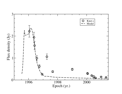
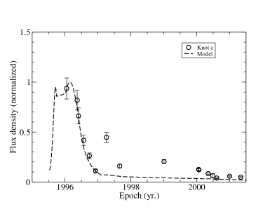
Figure 13: Knot-c. Left panel: the model-fit of the 15 GHz light curve with the modeled peak flux density of 2.37 Jy (at 1996.15) and the intrinsic flux density of 15.6 $\mu$Jy. Right panel: the light curve normalized by the modeled peak flux density is very well fitted by the Doppler-boosting profile $[\delta(t)/\delta_{max}]^{3+\alpha}$ with an assumed value $\alpha$=0.5. The data-points at 1997.26, 1997.66 and 1997.01 deviating from the Doppler-boosting profile obviously could be due to variations in its intrinsic flux density.

The model fit of the 15 GHz light curve is shown in Figure 13. The modeled peak flux density is 2.37 Jy (at 1996.15) and its intrinsic flux density 15.6$\mu$Jy. The light curve normalized by the modeled peak flux density is well fitted by the Doppler-boosting profile $[\delta(t)/\delta_{max}]^{3+\alpha}$ (with an assumed value $\alpha$=0.5). The flux fluctuations on shorter timescales (e.g. at 1997.26) which obviously deviate from the Doppler-boosting profile might be induced by the intrinsic flux variations of knot-c itself.

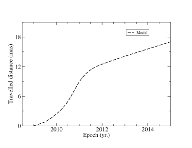
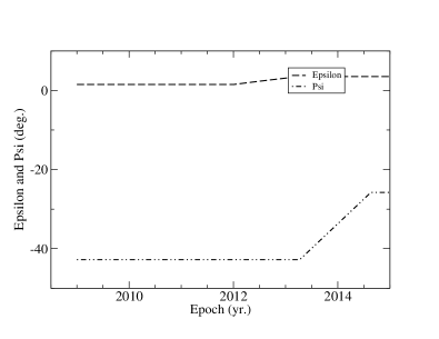
Figure 14: Knot-i. Left panel: the modeled traveled distance Z(t) along the jet-axis. Right panel: the modeled curves for parameters $\epsilon(t)$ and $\psi(t)$. Before 2012.0 (or Z(t) $\leq$12.5 mas=96.1 pc) $\epsilon$=$1.5^{\circ}$ and $\psi$=–$42.8^{\circ}$, knot-i moved along the precessing common trajectory. Beyond that distance its motion started to transfer to follow its own individual track, deviating from the precessing common trajectory.

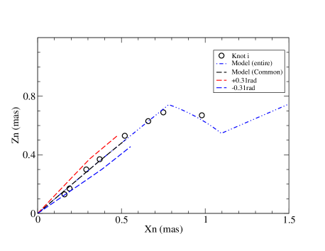
Figure 15: Knot-i: the model fit of the observed trajectory $Z_{n}(X_{n})$. Within coordinate $X_{n}{\simeq}$0.39 mas (Z$\leq$12.5 mas=96.1 pc), knot-i moved along the precessing common trajectory. Beyond that distance it started to follow its own individual track. The red and green curves are calculated for precession phases $\phi{\pm}$0.31 rad ($\phi$=1.0 rad), demonstrating that the observational data-points are within the area defined by the two curves and the precession period is determined correctly with an uncertainty of $\sim$${\pm}$5% of the precession period (or ${\sim}$$\pm$0.85 yr.).

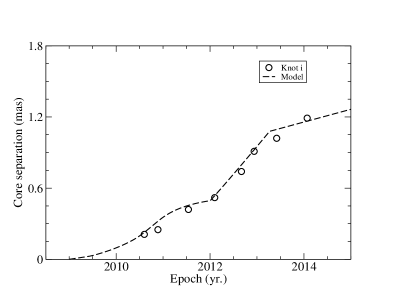
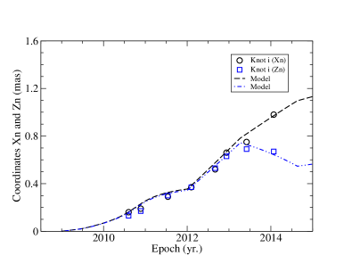
Figure 16: Knot-i. Left panel: the model fit of the core distance $r_{n}(t)$. Right panel: the model fits of the coordinates $X_{n}(t)$ and $Z_{n}(t)$. All the kinematic features are well fitted extending to $r_{n}\simeq$1.2 mas (during 2010.5–2014.5).

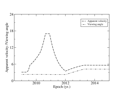
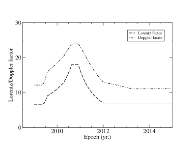
Figure 17: Knot-i. Left panel: the model-derived apparent velocity $\beta_{app}(t)$ and viewing angle $\theta(t)$. Right panel: the model-derived bulk Lorentz factor $\Gamma(t)$ and Doppler factor $\delta(t)$. $\beta_{app}(t)$, $\Gamma(t)$ and $\delta(t)$ all have a bump structure during 2009.5–2012.0, which was associated with a major burst (see Figure 18 below). At 2010.90 $\delta$= $\delta_{max}$=24.02 and $\Gamma$=$\Gamma_{max}$=13.80. At 2010.64 $\beta_{app}$=$\beta_{app,max}$=16.96. $\theta(t)$ varied in the range of [$2.27^{\circ}$, $4.18^{\circ}$] during 2009.5–2014.0.

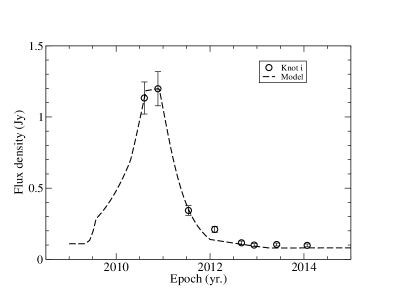
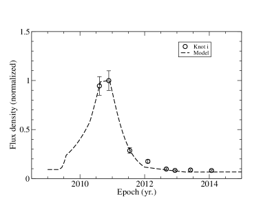
Figure 18: Knot-i. Left panel: the 15GHz light curve is well fitted with its modeled peak flux density of 1.20 Jy at 2010.90 and intrinsic flux density of 17.7$\mu$ Jy. Right panel: the light curve normalized by the modeled peak flux density is fitted very well by the Doppler-boosting profile $[\delta(t)/\delta_{max}]^{3+\alpha}$.

5 Knot i: Model-fitting results

The model-fitting results for knot-i are shown in Figures 14–18. Its ejection time $t_{0}$=2009.0 and the corresponding precession phase $\phi$=1.0 rad.

5.1 Knot-i: model-fit of kinematics

The modeled traveled distance Z(t) along the jet-axis and the modeled curves for parameters $\epsilon(t)$ and $\psi(t)$ are shown in Figure 14. Before 2012.00 (Z$\leq$12.5 mas=96.1 pc) $\epsilon$=$1.5^{\circ}$ and $\psi$=–$42.8^{\circ}$ knot-i moved along the precessing common trajectory, while after that $\epsilon$ increased knot-i started to move along its own individual track, deviating from the common precessing track ($\psi$ started to increase quickly after 2013.38).
The model fit of its projected trajectory $Z_{n}(X_{n})$ is shown in Figure 15. Within core separation $r_{n}$$\sim$0.49 mas knot-i moved along the common precessing track. Beyond that knot-i started to move along its own individual track, deviating from the common track. The red and green curves in the figure are calculated for precession phase $\phi{\pm}$0.31 rad ($\phi$=1.0 mas), indicating that the observational data-points are within the area defined by the two curves and the precession period is determined with an uncertainty of $\sim$${\pm}$5%.
Model fits of core separation $r_{n}(t)$ (left panel), coordinates $X_{n}(t)$ and $Z_{n}(t)$ are shown in Figure 16. Before 2012.00 ($r_{n}$$\leq$0.49 mas, $X_{n}$$\leq$0.39 mas) knot-c moved along the precessing common track, while after that knot-c stared to move along its own individual trajectory, deviating from the common precessing track. It can be seen that $r_{n}(t)$, $X_{n}(t)$ and $Z_{n}(t)$ are all well model-fitted during 2010.5–2014.0.
The model-derived apparent velocity $\beta_{app}(t)$, viewing angle $\theta(t)$, bulk Lorentz factor $\Gamma(t)$ and Doppler factor $\delta(t)$ are shown in figure 17. $\beta_{app}$, $\Gamma$ and $\delta$ all have a bump structure coincident with the radio burst (see Figure 18). At 2010.90 $\delta$=$\delta_{max}$=24.02, $\Gamma$=$\Gamma_{max}$=18.0. At 2010.64 $\beta_{app}$=$\beta_{app,max}$=16.94. $\theta(t)$ varied in the range of [$2.27^{\circ}$ (2009.0), $4.18^{\circ}$ (2014.0)].

5.2 Knot-i: flux evolution and Doppler-boosting effect

The model fit of the 15GHz light curve is shown in Fig.18 (left panel) with its modeled peak flux density 1.20 Jy (at 2010.90) and the intrinsic flux density 17.7$\mu$Jy. The light curve normalized by the modeled peak flux density was well fitted by its Doppler-boosting profile $[\delta(t)/\delta_{max}]^{3+\alpha}$ (right panel).

6 Knot k: Model-fitting results

The model fitting results of the kinematics and light curve for knot-k are shown in Figures 19–23. Its ejection time $t_{0}$=2010.88 and the corresponding precession phase $\phi$=0.30 rad.

6.1 Model-fitting of kinematics

The modeled traveled distance Z(t) along the jet-axis and the modeled curves for parameters $\epsilon(t)$ and $\psi(t)$ are shown in Figure 19. Before 2012.97 (or Z$\leq$7.2 mas=55.4 pc) $\epsilon$=$1.5^{\circ}$ and $\psi$=–$42.8^{\circ}$, knot-k moved along the precessing common track and after that $\epsilon$ decreased slightly knot-k started to move along its own individual track, slightly deviating from the precessing common trajectory.
The model-fit of the projected trajectory is shown in Figure 20. Within $X_{n}$=0.24 mas (or before 2012.97) knot-k moved along the precessing common track. Beyond that knot-k started to move along its own individual track, slightly deviating from the common precessing track. The red and green curves in the Figure are calculated for precession phases $\phi{\pm}$0.31 rad ($\phi$=0.30 rad), indicating that the observational data-points are within the area defined by the two curves and the precession period is determined with an uncertainty of $\sim$$\pm$5% of the period ($\sim$$\pm$0.85 years).
The model-fits of the core separation $r_{n}(t)$, coordinates $X_{n}(t)$ and $Z_{n}(t)$ are shown in Figure 21. Within $r_{n}$=0.26 mas (or $X_{n}$$\leq$0.24 mas; before 2012.97) knot-k moved along the precessing common track, while beyond that it started to move along its own individual track, deviating from the common track.
The model-derived apparent velocity $\beta_{app}(t)$, viewing angle $\theta(t)$, bulk Lorentz factor $\Gamma(t)$ and Doppler factor $\delta(t)$ are shown in Figure 22. $\beta_{app}$, $\Gamma$ and $\delta$ all have a bump structure: at 2013.00 $\delta$=$\delta_{max}$=24.50, $\Gamma$=16.06, $\beta_{app}$=13.62 and $\theta$=$1.99^{\circ}$. But $\Gamma_{max}$=16.50 (during 2012.81–2012.97) and $\beta_{app,max}$=14.4 (at 2012.81). Viewing angle $\theta(t)$ varied in the range of [$2.07^{\circ}$, $1.53^{\circ}$] during 2011.4–2014.0.

6.2 Knot k: flux evolution and Doppler-boosting effect

The model-fit of the 15 GHz light curve is shown in Fig.22 (left panel) with its modeled peak flux density 1.26 Jy (at 2013.00) and intrinsic flux density $S_{int}$=17.4 $\mu$Jy. The light curve normalized by the modeled peak flux density was well fitted by its Doppler-boosting profile $[\delta(t)/\delta_{max}]^{3+\alpha}$ with a presumed value $\alpha$=0.5 (right panel). The data-point at 2014.07, obviously deviating from the profile, might be due to the increasing of its intrinsic flux density.

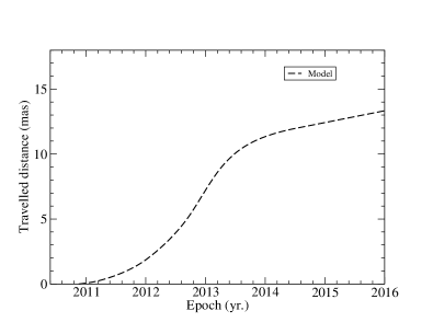
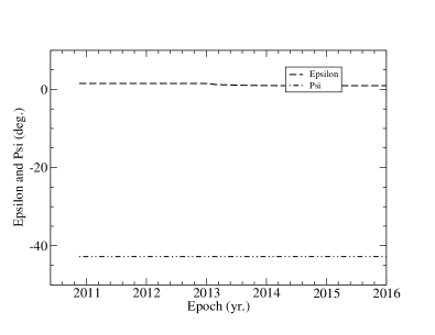
Figure 19: Knot-k. Left panel: the model-derived traveled distance Z(t). Right panel: the modeled curves of parameter $\epsilon(t)$ and $\psi(t)$. Before 2012.97 (corresponding to traveled distance Z$\leq$7.2 mas=55.4 pc) $\epsilon$=$1.5^{\circ}$ and $\psi$=–$42.8^{\circ}$, knot-k moved along the precessing common trajectory. After that epoch $\epsilon$ slightly decreased with time and knot-k started to move along its own individual trajectory, slighly deviating from the precessing common track.

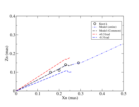
Figure 20: Knot-k: the model fit of the observed trajectory $Z_{n}(X_{n})$. Within $X_{n}{\leq}$0.24 mas (Z$\leq$7.2 mas=55.4 pc) knot-k moved along the preceessing common track. After that knot-k started to move along its own individual trajectory, deviating from the precessing common track. The red and green curves were calculated for the precession phases $\phi{\pm}$0.31 rad ($\phi$=0.30 rad), indicating that the observational data-points are within the area defined by the two curves and the precessing period is derived correctly with an uncertainty of $\sim$$\pm$5% of the period (or ${\sim}$$\pm$0.85 yr.).

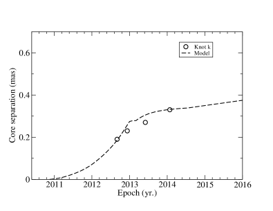
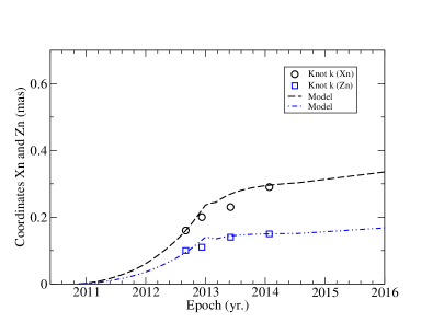
Figure 21: Knot-k. Left panel: the model fit of the core separation $r_{n}(t)$. Right panel: the model fits of the coordinates $X_{n}(t)$ and $Z_{n}(t)$. Before 2012.97 (or $r_{n}{\leq}0.26$ mas, $X_{n}{\leq}$0.24 mas) $\epsilon$=$1.5^{\circ}$ and $\psi$=–$42.8^{\circ}$, knot-k moved along the preceessing common track. After that knot-k started to move along its own individual trajectory, deviating from the precessing common track.

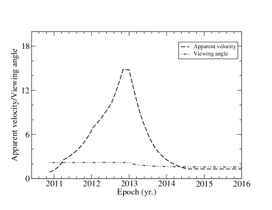
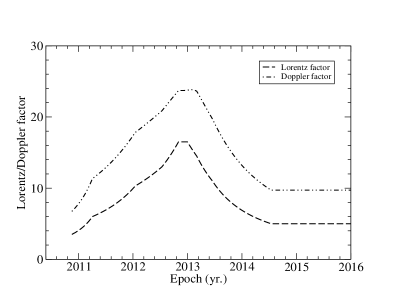
Figure 22: Knot-k. Left panel: the model-drived apparent velocity $\beta_{app}(t)$ and viewing angle $\theta(t)$. Right panel: the model-drived bulk Lorentz factor $\Gamma(t)$ and Doppler factor $\delta(t)$. At 2013.00 $\delta$= $\delta_{max}$=24.50, $\Gamma$=16.1 and $\beta_{app}$=13.6, while $\Gamma$=$\Gamma_{max}$=16.5 during 2012.81–2012.97 and $\beta_{app}$=$\beta_{app,max}$=14.4 at 2012.81. $\theta(t)$ varied in the range of [$2.07^{\circ}$, $1.53^{\circ}$] during 2011.4–2014.0.

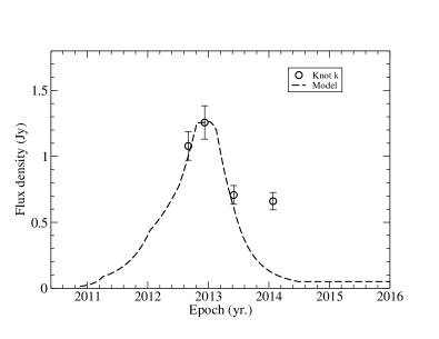
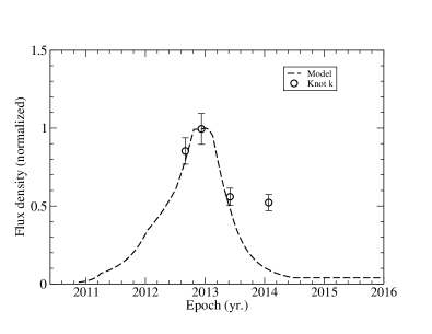
Figure 23: Knot-k. Left panel: the model fit of the 15 GHz light curve with its modeled peak flux density of 1.26 Jy (at 2013.0) and intrinsic flux density of 17.4 $\mu$Jy. Right panel: the light curve normalized by the modeled peak flux density is well fitted by the Doppler-boosting profile $[\delta(t)/\delta_{max}]^{3+\alpha}$ with an assumed $\alpha$=0.5. The data-point at 2014.07 deviating from the profile largely might be due to a variation in its intrinsic flux density.

7 Summary and conclusion

Based on our precessing jet-nozzle secnario (Qian et al. Qi17 (2017), Qi21 (2021)) we have successfully model-fitted the kinematics observed at 15 GHz on pc-scales for the three superluminal components (knot-c, -i and -k) in QSO B1308+326 and interpreted their light curves. We briefly summarize the results as follows:
(1) Superluminal components were ejected from the precessing jet-nozzle with a precession period of $\sim$16.9$\pm$0.85 years.
(2) The superluminal knots moved along the precessing common tracks corresponding to their precession phases (or ejection times) in the innermost jet regions (core separation $r_{n}\leq$0.30–0.5 mas), while in the outer jet-regions they started to deviate from the precessing common tracks and moved along their own individual trajectories.
(2) the periodic position angle swing observed for the superluminal components can be well explained in terms of our precessing nozzle scenario.
(3) The observed kinematic features (trajectory $Z_{n}(X_{n})$, core separation ($r_{n}(t)$), coordinates $X_{n}(t)$ and $Z_{n}(t)$ and apparent velocity $\beta_{app}(t)$) were consistently well model-fitted.
(4) The bulk Lorentz factor $\Gamma(t)$, viewing angle $\theta(t)$ and Doppler factor $\delta(t)$ for the superluminal components were properly derived.
(5) The 15 GHz light curves of the superluminal components can be well interpreted in terms of their Doppler-boosting effect.
Our precessing jet-nozzle scenario may be described by such a physically feasible conception:
In the nucleus of B1308+328 there is a energy-engine consisting of a rotating (Kerr) black-hole and a tilted magnetized accretion-disk around the hole. Due to the electromagnetic effects induced from the spin of the black hole and the rotation of the disk with its magnetosphere, a mini-jet (or beam) is formed with a nozzle steadily ejecting magnetized plasma and superluminal plasmoids along helical tracks around the axis of the disk. Moreover, due to the frame-dragging effect the gravitational torque of the rotating black hole will cause a global precession of the accretion disk with its mini-jet. Thus the precession of the mini-jet would naturally form the precessing common trajectory suggested in our scenario, producing the observed periodic position angle swing of superlumnal components and regular distribution of their inner trajectories. Obviously, in our scenario, the observed jet (as usually defined) is originated from the precession of the single mini-jet which ejects magnetized plasma and superlumnal plasmoids in a long period.
Our precessing nozzle scenario can be understood in the framework of available relativistic magnetohydrodynamic theories for the formation/collimation/acceleration of relativistic jets in blazars (cf. a detailed discussion in Qian et al. Qi17 (2017)). The structure of the jets observed in the radio galaxy M87 (parabolic hollow jet nozzle structure; Nakamura & Asada Na13 (2013)) and in OJ287 (fork-like jet structure; Tateyama Ta13 (2013)) may be regarded as observational evidence.
Theoretically, magnetic nozzles can be probably formed in disk-driven jets in the magnetospheres of rotating black-hole/accretion-disk systems. These magnetic nozzles may locate near the classical fast magnetosonic point where the magnetohydrodynamic flow remains Poynting flux dominated. In some self-similar axisymmetric MHD flow models, beyond the classic fast magnetosonic point, the jet will be accelerated untill approaching the modified fast magnetosonic point (Blandford & Znajek Bl77 (1977); Li et al. Li92 (1992); Vlahakis & Königl Vl04 (2004)). This extended acceleration is due to the dominance of Poynting flux at the classic magnetosonic point, thus having ample electromagnetic energy to be transformed plasma kinetic energy (Komissarov et al. Kom07 (2007), Komissarov Kom09 (2009), Millas et al. Mi14 (2014)).
. In the case of relativistic jets, the classical fast magnetosonic point is located in the force-free region of the magnetosphere where the magnetic energy dominates the plasma kinetic energy. The magnetic field lines anchored into the innermost disk and the magnetic nozzle would rotate rigidly with the disk (MacDonald & Throne Mac82 (1982)).
Additionally, in this extended acceleration region beyond the magnetic nozzle (or beyond the classical fast magnetosonic point), the inertia of the plasma becomes strong and the electromagnetic fields are neither degenerate nor force free, and the plasma would flow along its own streamlines, not following the local field lines and forming its own trajectory pattern. This can explain why the superluminal knots observed in B1308+326 move along the common precessing track.
Most recently, the black-hole/accretion-disk system in the giant radio galaxy M87 (having a hole-mass of $\sim$6.5$\times{10^{9}}$$M_{\odot}$) has been observed by using the world mm-VLBI-network (Lu et al. Lu23 (2023)). Both the mm-jet emanating from its centeral hole and the associated circumdisk structure have been mapped. The morphological strcuture and kinematic properties are well consistent with the whole picture expected by relativistic MHD theories for jet formation in black-hole/accretion disk systems.

References

- (1) Acero, F., Ackermann, M., Ajello, M., et al. 2015, ApJS, 218, 23
- (2) Ackermann, M., Ajello, M., Allafort, A., et al. 2011, ApJ, 743, 171
- (3) Angel, J.R.P., & Stockman, H.S. 1980, Ann. Rev. Astron. Astrophys., 8, 321
- (4) Asada, K., & Nakamura, M. 2012, ApJL, 745, L28
- (5) Beskin, V.S., & Zheltoukhov, A.A. 2013, Astronomy Letters, 39, 215
- (6) Biretta, J.A., Junor, W., & Livio, M. 2002, New Astronomy Review (NAR), 46,239
- (7) Blandford, R.D., & Znajek, R.L. 1977, MNRAS, 179, 433
- (8) Britzen, S., Qian, S.J., Steffen, W., et al. 2017, A&A, 602, A29
- (9) Doeleman, S.S., Fish, V.L., Schenck, D.E., et al. 2012, Science, 338, 355
- (10) Falcke H., Wilson A.S., Simpson C., Bower G.A., 1996, ApJ 470, L31
- (11) Hardee, P. E. 1987, ApJ, 318, 78
- (12) Hardee P.E., 2011, in Jets at all Scales, Proceedings of the International Astronomy Union, IAU Symposium 275, 41–49
- (13) Hogg, D. W. 1999, astro-ph/9905116
- (14) Kim J.Y., Savolainen T., Voitsik P., et al. 2023, arXiv e-prints, arXiv:2304.09816 [astro-ph.GA]
- (15) Komissarov, S.S., Barkov, M.V., Vlahakis, N., & Königl, A. 2007, MNRAS, 380, 51
- (16) Komissarov, S.S. 2009, Journal of the Korean Physical Society (JKPS), 54, 2503
- (17) Li, Z.Y., Chieuh, Z.H., & Begelman, M.C. 1992, ApJ, 394, 459
- (18) Lister, M.L., Cohen, M.H., Homan, D.C., et al. 2009, AJ, 138, 3718
- (19) Lu R.S., Asada K., Krichbaum t.P., et al., 2023, Nature 616 , 686-690
- (20) Macdonald, D., & Thorne, K.S. 1982, MNRAS, 198, 345
- (21) McKinney, J.C., Tchekhovskoy, A., & Blandford, R.D. 2012, MNRAS, 423, 2083
- (22) Milas, D., Katsoulakos, G., Lingri, D., et al. 2014, in High Energy Phenomena in Relativistic Outflows (International Journal of Modern Physics Conference series vol.28, id 1460200)
- (23) Nakamura, M. & Asada, K. 2013, ApJ, 775, 118
- (24) Nakamura M. & Meier D.L., 2004, ApJ 617, 123
- (25) Pen, Ue-Li. 1999, ApJS, 120, 49
- (26) Punsly, B. 2001, Black Hole Gravitohydromagnetics (New York: Springer)
- (27) Qian, S. J., Witzel, A., Krichbaum, T., et al. 1991, Acta Astron. Sin., 32, 369 (english translation: in Chin. Astro. Astrophys., 16, 137 (1992))
- (28) Qian, S.J. 2012, RAA, 12, 46
- (29) Qian, S.J. 2013, RAA, 13, 783
- (30) Qian, S.J., Britzen, S., Witzel, A., et al. 2014, RAA, 14, 249
- (31) Qian, S. J. 2016, RAA, 16, 20
- (32) Qian, S.J., Britzen S., Witzel, A. et al. 2017, A&A, 604, A90
- (33) Qian, S.J., Britzen S., Witzel, A. et al. 2018a, A&A, 615, A123
- (34) Qian S.J., 2018b, arXiv e-prints, arXiv:1811.1154 [astro-ph.GA]
- (35) Qian, S., Britzen S., Krichbaum T.P., Witzel A., 2019, A&A, 621, A11
- (36) Qian S.J., Britzen S., Krichbaum T.P., Witzel A., 2021, A&A, 653, A7
- (37) Qian S.J., 2022a, arXiv e-prints, arXiv:2202.01915 [astro-ph.GA]
- (38) Qian S.J., 2022b, arXiv e-prints, arXiv:2206.14995 [astro-ph.GA]
- (39) Spergel, D. N., Verde, L., Peiris, H. V., et al. 2003, ApJS, 148, 175
- (40) Tateyama, C. E., & Kingham, K. A. 2004, ApJ, 608, 149
- (41) Tateyama, C.E. 2009, ApJ, 705, 877
- (42) Tateyama, C.E. 2013, ApJS, 205, 15
- (43) Vlahakis, N., & Königl, A. 2004, ApJ, 605, 656