Spatial Re-parameterization for N:M Sparsity

Abstract

This paper presents a Spatial Re-parameterization (SpRe) method for the N:M sparsity in CNNs. SpRe is stemmed from an observation regarding the restricted variety in spatial sparsity present in N:M sparsity compared with unstructured sparsity. Particularly, N:M sparsity exhibits a fixed sparsity rate within the spatial domains due to its distinctive pattern that mandates N non-zero components among M successive weights in the input channel dimension of convolution filters. On the contrary, we observe that unstructured sparsity displays a substantial divergence in sparsity across the spatial domains, which we experimentally verified to be very crucial for its robust performance retention compared with N:M sparsity. Therefore, SpRe employs the spatial-sparsity distribution of unstructured sparsity to assign an extra branch in conjunction with the original N:M branch at training time, which allows the N:M sparse network to sustain a similar distribution of spatial sparsity with unstructured sparsity. During inference, the extra branch can be further re-parameterized into the main N:M branch, without exerting any distortion on the sparse pattern or additional computation costs. SpRe has achieved a commendable feat by matching the performance of N:M sparsity methods with state-of-the-art unstructured sparsity methods across various benchmarks. Code and models are anonymously available at https://github.com/zyxxmu/SpRe.

1 Introduction

Network sparsity has proven highly successful in reducing the complexity of Convolutional Neural Networks (CNNs) [11, 19, 25]. Concretely speaking, a sparse network can be obtained by pruning weights at different levels of granularity, from fine to coarse. Fine-grained sparsity (unstructured sparsity) [19, 7] prunes at the level of each individual weight, enabling a negligible performance drop even at high sparsity rates. Unfortunately, the deployment of fine-grained sparse networks on off-the-shelf hardware is cumbersome due to the irregularity of sparse weight matrices. On the other hand, coarse-grained sparsity (structured sparsity) [14, 21] achieves significant acceleration by eliminating entire convolution filters [24, 21] or weight blocks [16, 26], yet suffers severe performance degradation under high sparsity rates.

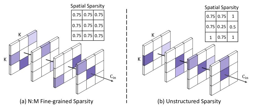
Figure 1: A toy example of the discrepancy in spatial sparsity between N:M sparsity at 1:4 pattern and unstructured sparsity at 75% sparsity rate. (a) N:M sparsity requires N non-zero components among M consecutive weights in the input channel dimension, resulting in equal spatial sparsity. (b) Unstructured sparsity removes weights at arbitrary locations, resulting in uneven spatial sparsity.

N:M sparsity has lately surfaced as a promising direction of augmenting the trade-off between acceleration effects and performance retention [36, 30]. By stipulating N non-zero components within M consecutive weights across the input channel dimension, it considerably improves the performance of structured sparsity while simultaneously ensuring expeditious inference aided by the N:M sparse tensor core [28]. In recent years, various methods have been proposed to train N:M sparse networks from pre-trained weights [28, 30] or randomly-initialized weights [36, 35]. In spite of the continuous progress, the efficacy of N:M sparsity concerning performance retention still lags behind unstructured sparsity, particularly at high sparsity rates such as 95% [23, 36]. We ask: what causes the performance gap between N:M sparsity and unstructured sparsity?

In this paper, we address this inquiry through empirical observation of network sparsity over the spatial domain, i.e., spatial sparsity. Particularly, N:M sparsity displays a consistent sparsity rate of $1-\frac{\text{N}}{\text{M}}$ at every spatial location of convolution filters owing to the distinctive sparse pattern depicted in the input channel dimension (Fig. 1a). Conversely, unstructured sparsity can exhibit a notable variation in spatial sparsity (Fig. 1b), which we confirm to be ubiquitous in existing unstructured sparsity methods and crucial for their robust performance retention compared with N:M sparsity methods (Sec. 3.2). To explain this, a heterogeneous distribution of weights across various positions aids in giving precedence to the most informative visual elements in the spatial domain, consequently resulting in enhanced performance for the sparse networks. Self-evidently, N:M sparsity falters to assign adequate weights for the informative visual elements especially when the sparsity rate is high, therefore leading to more performance degradation.

Driven by this analysis, we present Spatial Re-parameterization (SpRe) as a way of matching the performance between N:M sparsity and unstructured sparsity. SpRe utilizes the spatial sparsity distribution of unstructured sparsity to allocate an extra weight branch in conjunction with the original N:M sparse weights. This enables the N:M sparse network to maintain a sparsity distribution comparable to that of unstructured sparsity. Moreover, we constrain the newly introduced parameters to adhere to the N:M sparse distribution of the main branch in the input channel dimension. This results in an advantage for a re-parameterization after training, where the newly-added branch can be merged into the main block without impacting the output at inference stage. Thus, SpRe introduces no additional inference burden for the original N:M sparse networks. The advantages of our proposed SpRe include:

• Trackable. SpRE is traceable in principle, due to our innovative observation of the discrepancy in spatial sparsity between N:M sparsity and unstructured sparsity.

• Scalable. SpRe is easy to use and orthogonal to other methods of N:M sparsity, whether applied from randomly-initialized or pre-trained weights.

• High-performance. SpRe is validated to be highly successful in boosting the performance of N:M sparsity methods across various benchmarks. Specifically, SpRe enhances the top-1 accuracy of SR-STE [36], a leading N:M method, by 1.2% when training a 1:16 sparse ResNet-50 [13] on ImageNet [1]. Moreover, the boosted performance even surpasses state-of-the-art unstructured sparsity method GraNet [23] by 0.4% at a similar sparsity rate.

2 Related Work

Unstructured Sparsity. Unstructured sparsity removes individual weights at arbitrary positions of the network. Gradient [20], momentum [7] and magnitude [11] are often used to identify and remove insignificant weights. Recent advancements learn to train an unstructured sparse network. RigL [8] alternatively removes and revives weights based on magnitudes and gradients. Sparse Momentum [2] considers the mean momentum magnitude in each layer to redistribute weights. Besides, gradual sparsity is widely adopted to boost performance [37, 23]. Unstructured sparsity is demonstrated to well retain performance, even at a very high sparsity over 95% [23]. However, it defects in the resulting irregular sparse tensors that gain rare speedups on general hardware [33].

N:M Sparsity. N:M sparsity preserves N out of M consecutive weights along the input channel dimension of CNNs, and achieves practical speedups thanks to the hardware innovation of N:M sparse tensor core [28, 9]. The pioneering ASP [28] goes through model pre-training, high-magnitude weight removal [11], and model fine-tuning. Pool et al. [30] proposed channel permutation to increase performance of ASP. Sun et al. [31] proposed a layerwise fine-grained N:M sparsity to replace the common uniform version. To avoid heavy burden on model pre-training, Zhou et al. [36] proposed a sparse-refined straight-through estimator (SR-STE) to learn from scratch. LBC [35] further forms the N:M sparsity as a combinatorial problem and learns the best combination for the sparse weights.

Structural Re-parameterization. Structural re-parameterization mutually converts different architectures through an equivalent transformation of parameters. The representative RepVGG [6] merges kernels of smaller sizes to these of larger ones in inference. For example, 1$\times$1 kernels can be added onto the central points of the 3$\times$3 kernels. Along this line, researchers have devised various blocks to boost the performance of a regular CNN without extra inference costs, e.g., Asymmetric Convolution Block (ACB)  [3], RepLKNet [5]. Besides, structural re-parameterization is also leveraged to guide channel pruning [4], where the original CNN is re-parameterized into two parts to respectively maintain the performance and prune convolutional filters.

We focus on developing an N:M sparsity method that is orthogonal to the aforementioned methods for performance improvement, simply due to two advantages of our method: First, we utilize the distribution of unstructured sparsity across the spatial domain. Second, we re-parameterize a newly-added branch into the main branch of N:M block in the inference.

3 Methodology

3.1 Background

For convolutional weights $\mathbf{W}\in\mathbb{R}^{C_{o}\times C_{i}\times K\times K}$ ($C_{o}$: output channel, $C_{i}$: input channel, $K$: kernel size), the convolution operation with input features $\mathbf{X}\in\mathbb{R}^{H\times W\times C_{i}}$ ($H$: height, $W$: width) is generally formulated as:

$$\mathbf{Y}=BN(\mathbf{W}\circledast\mathbf{X}),$$ (1)

where $\circledast$ represents convolution operation and $BN(\cdot)$ stands for the follow-up batch normalization. Network sparsity can be realized with a $0$-$1$ mask $\mathbf{B}$ of the same shape to $\mathbf{W}$:

$$\mathbf{Y}=BN((\mathbf{B}\odot\mathbf{W})\circledast\mathbf{X}),$$ (2)

where $\odot$ denotes the element-wise multiplication. Therefore, $\mathbf{B}_{p,q,u,v}$ = $0$ removes $\mathbf{W}_{p,q,u,v}$ and $\mathbf{B}_{p,q,u,v}$ = $1$ preserves $\mathbf{W}_{p,q,u,v}$.

For unstructured sparsity, the zero entries are irregular in the positions of $\mathbf{B}$. Instead, N:M sparsity stipulates at N non-zero entries for every M consecutive weights along the input channel dimension. Therefore, $\mathbf{B}$ is restricted to satisfy:

$${\|\mathbf{B}_{p,\lfloor q/\text{M}\rfloor\cdot\text{M}:\lfloor q/\text{M}\rfloor\cdot\text{M}+\text{M},u,v}\|}_{0}=\text{N},$$ (3)

where $p,q,u,v$ enumerates $C_{o},C_{i},K,K$, respectively.

Besides, for ease of the following representation, we define Spatial Sparsity (SS) to measure the weight sparsity in the spatial domain. The spatial sparsity at location ($u$, $v$) is calculated as:

$$\text{SS}(\mathbf{B},u,v)=1-\frac{1}{C_{o}\cdot C_{i}}\sum_{p=1}^{C_{o}}\sum_{q=1}^{C_{i}}\mathbf{B}_{p,q,u,v}.$$ (4)

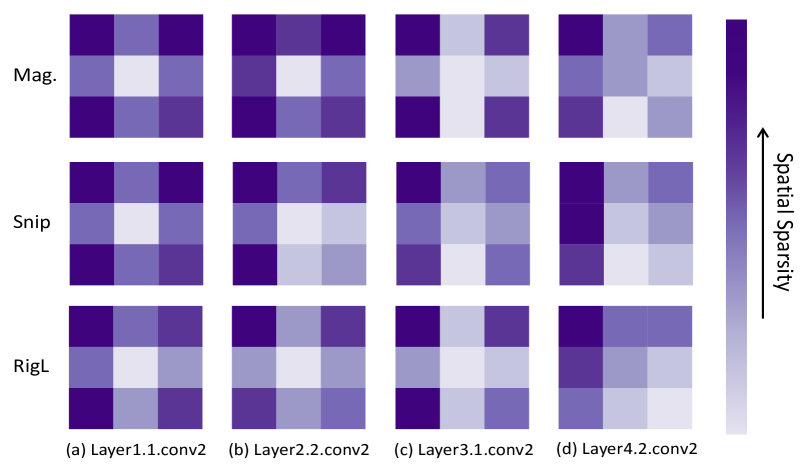
Figure 2: Spatial sparsity of common unstructured sparsity methods including Magnitude-based sparsity [11], RigL [8], GraNet [23]. We show spatial sparsity of 3$\times$3 kernels from different layers of ResNet-50 [13] with overall 95% sparsity, close to the sparsity level of 1:16 pattern. Experiments are performed on ImageNet-1K [1].

3.2 Discrepancy in Spatial Sparsity

Compared to unstructured sparsity, N:M sparsity achieves practical speedups with the support of the N:M sparse tensor core [28, 9], yet it suffers more performance degradation, particularly at high sparsity rates [36, 23]. In this section, we demonstrate that such a performance gap comes from a discrepancy in the spatial sparsity between N:M sparsity and unstructured sparsity. Simply due to the constraint of Eq. (3), N:M sparsity possesses consistent spatial sparsity across different positions and layers as

$$\text{SS}(\mathbf{B},u,v)=1-\frac{\text{N}}{\text{M}}.$$ (5)

In other words, N:M sparsity equally allocates weights across the spatial domain of convolution operation. On the other hand, such balanced spatial sparsity is not imperative for unstructured sparsity, given that no sparsity restriction is imposed across the channel dimension. Indeed, we observe that unstructured sparsity exhibits significant variability in terms of spatial sparsity, as illustrated by Fig. 2. This variability in spatial sparsity remains consistent across different layers and network types, irrespective of the specific unstructured sparsity technique employed [11, 8, 27].

Upon closer examination of Fig. 2, it can be inferred that the majority of unstructured weights even maintain a similar distribution spatial sparsity, more interestingly resembling a cross-like configuration in the shallow layers. This intriguing phenomenon warrants further exploration and investigation within the domain of unstructured sparsity. We do not delve deeply into this matter at present, but it is unequivocal that unstructured sparsity methods [11, 8, 27] allocate more weights to certain fixed visual points simultaneously.

CNNs analyze visual imagery by sliding filters along input features to empower each weight to interact with different visual regions. We conjecture that unstructured sparsity methods implicitly acquire weights in the spatial domain that can better tell importance of input visual regions, such that the sparse network learns to focus more on crucial visual areas. To verify our hypothesis, we destroy the variable spatial sparsity of the state-of-the-art unstructured sparsity method GraNet [23] by constraining the sparsity at any location ($u$, $v$) to be the same. Fig. 3 manifests the performance comparison. We can observe performance degenerates a lot, even close to the N:M method SR-STE [36], when the spatial sparsity variability crashes. Therefore, we can ascertain that the variable spatial sparsity is the key to the impressive performance of unstructured sparsity methods. From here we can also see that how to develop an enhancement policy to reimburse the spatial sparsity variability is the core to improve the performance of N:M methods.

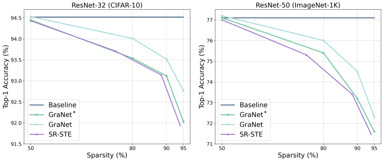
Figure 3: Performance comparison of sparse ResNet-50 [13] on ImageNet-1K [1] and ResNet-32 [13] on CIFAR-10 [17]. The involved methods include the dense version of ResNet-50 (Baseline), SR-STE [36] (N:M sparsity), unstructured sparse GraNet [23] and GraNet with the same spatial sparsity along the spatial dimension (GraNet^⋆). Performance drops when unstructured sparse method is confined to having the same spatial sparsity.

3.3 Spatial Re-parameterization

Based on the aforementioned analysis, we propose Spatial Re-parameterization (SpRe) as a way of attaining comparable performance to that of N:M sparsity and unstructured sparsity. To address the issue of limited variation in spatial sparsity observed in N:M sparsity, SpRe introduces an extra branch $\mathbf{B}^{S}\odot\mathbf{W}^{S}$ in conjunction with the original N:M sparse weights $\mathbf{B}\odot\mathbf{W}$ (Fig. 4). In particular, we first obtain mask $\mathbf{B}^{U}$ of unstructured sparsity with a sparsity rate $P=1-\frac{\text{N}}{\text{M}}$. Here we utilize the classic magnitude-based pruning [11], while other metrics for unstructured sparsity [27, 20, 32] can also adapt well. As previously shown in Eq. (5), the N:M weights $\mathbf{B}\odot\mathbf{W}$ maintain a constant spatial sparsity of rate $1-\frac{\text{N}}{\text{M}}$. Therefore, in the extra branch, we allocate parameters at spatial locations where unstructured sparsity exhibits less spatial sparsity than N:M sparsity as

$$\mathbf{B}^{S}_{:,:,u,v}=\left\{\begin{array}[]{ll}\mathbf{B}_{:,:,u,v},\;\textrm{if}\;\text{SS}(\mathbf{B}^{U},u,v)<1-\frac{\text{N}}{\text{M}},\\ 0,\;\textrm{otherwise,}\end{array}\right.$$ (6)

in which $u=1,...,K,v=1,...,K$. In terms of formula, the forward propagation of SpRe in the training stage for N:M sparsity can be expressed as

$$\mathbf{Y}=BN((\mathbf{B}\odot\mathbf{W})\circledast\mathbf{X})+BN((\mathbf{B}^{S}\odot\mathbf{W}^{S})\circledast\mathbf{X}).$$ (7)

In this manner, the spatial sparsity of N:M sparsity is reimbursed to a comparable level of unstructured sparsity during training. Moreover, the extra branch can be re-parameterized into the main branch without incurring additional inference burden. Particularly, the BN layer can be firstly merged into the convolution layer [6]. Then, the final N:M sparse weights are obtained by adding up the weights of the extra branch and the main branch in a point-wise manner. As $\mathbf{B}^{S}$ is a subset of $\mathbf{B}$ according to Eq. (6), neither interference on the N:M pattern nor extra inference burden is introduced by SpRe. Eventually, the forward propagation after sparse training returns to its original N:M form as:

$$\mathbf{Y}=(\mathbf{B}\odot\bar{\mathbf{W}})\circledast\mathbf{X},$$ (8)

where $\bar{\mathbf{W}}$ represents the merged weight.

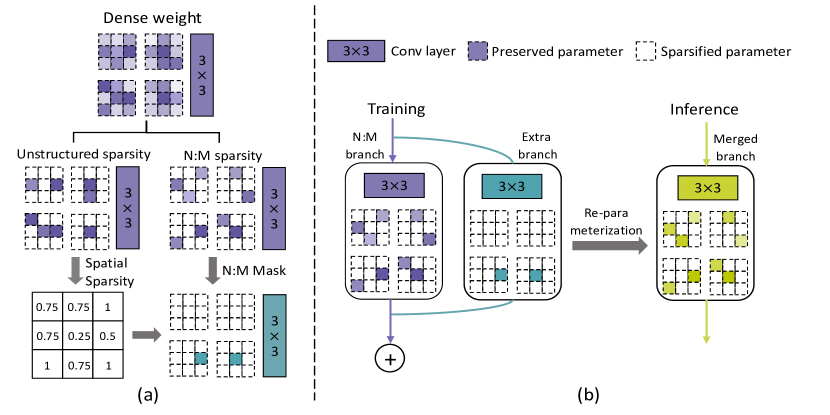
Figure 4: Framework of the proposed SpRe. (a) An extra branch is built upon the spatial sparsity arising from unstructured sparse weights and the N:M sparse mask (Eq. (6)). (b) The extra branch is trained in conjunction with the main N:M branch to reimburse the spatial sparsity. After training, a re-parameterization is performed to merge these two branches, without altering the output.

Implementation of SpRe. SpRe is orthogonal to existing N:M sparsity techniques and can be effortlessly employed to enhance their lack of spatial sparsity variety. For techniques that attain N:M sparsity after pre-training the dense weights [11, 30], SpRe can be directly applied to build the re-parameterization branch on the basis of pre-trained weights. After fine-tuning, the re-parameterization is employed to derive the N:M sparse weights for inference. For methods that excavate N:M sparsity from scratch in a sparse training manner [36, 35], SpRe can also dynamically adapt the binary mask $\mathbf{B}^{S}$ of the extra branch by looking at the updated weights during training. This ensures that the extra branch can simultaneously sustain proper spatial sparsity distribution and re-parameterization capability. As a result, SpRe can be readily integrated into existing N:M sparsity methods to gain a consistent enhancement in their performance, which is experimentally substantiated in the subsequent section.

4 Experiments

4.1 Settings

Our experiments include image classification on the CIFAR-10 [17] and ImageNet-1K datasets [1], object detection and instance segmentation on the COCO benchmark [22]. The specific settings are respectively expounded as follows. We validate the efficacy of SpRe in elevating the performance of prominent N:M sparsity methods, including ASP [28], SR-STE [36], and LBC [35]. We keep the same training configuration as their original implementation for a fair comparison. Our experiments cover a wide range of N:M patterns including 2:4, 1:4, and 1:16. For image classification, we sparsify ResNet-32 [13] on CIFAR-10 dataset, and ResNet-18 [13], ResNet-50 [13], MobileNet-V1 [15] on ImageNet-1K dataset. Besides, we exploit the efficacy of SpRe to aid SR-STE [36] in training 2:4 and 2:8 sparse Faster RCNN [10] for object detection and Mask RCNN [12] for instance segmentation, utilizing ResNet-50 as the backbone. We employ SpRe to all N:M weights except for 1$\times$ 1 kernels wherein the notion of spatial sparsity is deemed inapplicable. Our experiments are implemented with PyTorch [29] and run on NVIDIA Tesla A100 GPUs.

Table 1: Results for sparsifying ResNet-32 on CIFAR-10.

Model	Method	N:M	Top-1 Acc	N:M	Top-1 Acc	N:M	Top-1 Acc
ResNet-32	Baseline	-	95.2	-	95.2	-	95.2
ResNet-32	ASP [28]	2:4	95.0	1:4	94.3	1:16	92.6
ResNet-32	+SpRe	2:4	95.1(+0.1)	1:4	94.7(+0.4)	1:16	93.7(+1.1)
ResNet-32	SR-STE [36]	2:4	94.9	1:4	94.3	1:16	92.6
ResNet-32	+SpRe	2:4	95.1(+0.2)	1:4	94.6(+0.3)	1:16	93.9(+1.3)

Table 2: Results for sparsifying ResNet-18 on ImagNet-1K.

Model	Method	N:M	Top-1 Acc	N:M	Top-1 Acc	N:M	Top-1 Acc
ResNet-18	Baseline	-	70.9	-	70.9	-	70.9
ResNet-18	ASP [28]	2:4	70.6	1:4	69.1	1:16	65.0
ResNet-18	+SpRe	2:4	70.8(+0.2)	1:4	69.6(+0.5)	1:16	65.5(+0.4)
ResNet-18	SR-STE [36]	2:4	71.2	1:4	69.2	1:16	64.9
ResNet-18	+SpRe	2:4	71.3(+0.1)	1:4	69.9(+0.7)	1:16	65.7(+0.8)

Table 3: Results for sparsifying ResNet-50 on ImagNet-1K.

Model	Method	N:M	Top-1 Acc	N:M	Top-1 Acc	N:M	Top-1 Acc
ResNet-50	Baseline	-	77.2	-	77.2	-	77.2
ResNet-50	ASP [28]	2:4	77.4	1:4	76.5	1:16	71.5
ResNet-50	+SpRe	2:4	77.7(+0.3)	1:4	76.8(+0.3)	1:16	72.3(+0.8)
ResNet-50	SR-STE [36]	2:4	77.0	1:4	75.3	1:16	71.5
ResNet-50	+SpRe	2:4	77.2(+0.2)	1:4	76.1(+0.8)	1:16	72.7(+1.2)
ResNet-50	LBC [35]	2:4	77.2	1:4	75.9	1:16	71.8
ResNet-50	+SpRe	2:4	77.3(+0.1)	1:4	76.4(+0.5)	1:16	72.9(+1.1)

Table 4: Results for sparsifying MobileNet-V1 on ImageNet-1K.

Model	Method	N:M	Top-1 Acc	N:M	Top-1 Acc	N:M	Top-1 Acc
MobileNet-V1	Baseline	-	71.9	-	71.9	-	71.9
MobileNet-V1	ASP [28]	2:4	70.2	1:4	63.9	1:16	50.4
MobileNet-V1	+SpRe	2:4	70.5(+0.3)	1:4	66.6(+2.5)	1:16	58.0(+7.6)
MobileNet-V1	SR-STE [36]	2:4	70.4	1:4	63.2	1:16	25.4
MobileNet-V1	+SpRe	2:4	70.8(+0.4)	1:4	64.9(+1.7)	1:16	34.2(+8.8)

Table 5: Results of the N:M and unstructured sparsity methods for sparsifying ResNet-50.

Model	Method	Sparsity	Top-1 Acc	Sparsity	Top-1 Acc	Structured
ResNet-50	DNW [34]	90	74.0	95	68.3	✗
ResNet-50	RigL [8]	90	73.0	95	70.0	✗
ResNet-50	GMP [37]	90	73.9	95	70.6	✗
ResNet-50	STR [18]	91	74.0	95	70.4	✗
ResNet-50	GraNet [23]	90	74.2	95	72.3	✗
ResNet-50	SR-STE [36]	88(1:8)	73.8	94(1:16)	71.5	✓
ResNet-50	+SpRe	88(1:8)	74.7(+0.9)	94(1:16)	72.7(+1.2)	✓
ResNet-50	LBC [35]	88(1:8)	74.0	94(1:16)	71.8	✓
ResNet-50	+SpRe	88(1:8)	74.8(+0.8)	94(1:16)	72.9(+1.1)	✓

4.2 Image Classification

We first evaluate the efficacy of SpRe for sparsifying ResNet-32 on the CIFAR-10 dataset, which includes 50,000 training images and 10,000 validation images within 10 classes. Tab. 1 shows that SpRe can be effortlessly leveraged to enhance the performance of N:M methods. For instance, the top-1 classification accuracy of SR-STE is improved by 0.2%, 0.3%, and 0.9% for 2:4, 1:4, and 1:16 patterns, respectively. Given that no extra inference burden is introduced, the effectiveness of SpRe for N:M sparsity is obvious.

For the large-scale ImageNet-1K dataset that contains over 1.2 million images for training and 50,000 images for validation in 1,000 categories, we first present the quantitative results for sparsifying ResNet [13] with depths of 18 and 50 in Tab. 3. Encouragingly, SpRe substantially enlarges the performance of N:M methods over a wide range of sparse patterns. Without extra inference burden introduced, $0.2\%$ and $0.5\%$ top-1 accuracy improvements are gained by equipping ASP [28] with SpRe when sparsifying ResNet-18 at 2:4 and 1:4 patterns. The advantage of SpRe becomes more pronounced with an increase in the sparsity rate, where classic N:M sparsity methods fail to allocate enough weights for processing the important visual points due to a constant spatial sparsity. Upon training 1:16 sparse ResNet-50, SpRe exhibits a remarkable enhancement in the top-1 accuracy of SR-STE [36] and LBC [35] by 1.2% and 1.1%, respectively. This improvement can be intuitively attributed to compensation for the absence of weight preservation at crucial visual locations.

Furthermore, we examine the generalization capability of SpRe for sparsifying MobileNet-V1 [15], a lightweight network incorporating depth-wise convolution design and poses more challenges for compression. Tab. 4 demonstrates a distinct trend whereby the performance improvements achieved by SpRe remain consistent and increase as the sparsity level increases, irrespective of the specific N:M methods employed. For instance, SpRe is able to enhance the top-1 accuracy of ASP by $0.3\%$, $2.5\%$, and $7.6\%$ at 2:4, 1:4, 1:16 sparse patterns, respectively. These results well highlight the efficacy of SpRe in advancing existing N:M sparsity methods for sparsifying light-weight networks.

Additionally, we provide the performance comparison between unstructured sparsity and N:M sparsity methods in Tab. 5. The results reveal that N:M sparsity methods struggle to maintain accuracy on par with advanced unstructured sparsity techniques at comparable levels of sparsity. This disparity in performance can be attributed to the fact that unstructured sparsity, as we previously discussed, sustains adequate processing of crucial visual points at high levels of sparsity. In contrast, N:M sparsity fails to effectively handle this aspect due to its constant spatial sparsity and hence lags behind in achieving comparable outcomes. Fortunately, by allocating re-parameterizable weights that follow the spatial sparsity distribution of unstructured sparsity, SpRe effectively elevates the accuracy of N:M sparsity methods to the level of state-of-the-art unstructured sparsity methods without incurring any extra inference overhead. For instance, SR-STE surpassed the recent unstructured sparsity method GraNet [23] by 0.4% top-1 accuracy with the aid of SpRe (72.7% for SR-STE boosted by SpRe and 72.3% for GraNet at similar sparsity rates). Given the distinct advantage of N:M sparsity for practical acceleration on the N:M sparse tensor core, the significance of SpRe in bridging the performance gap between N:M sparsity and unstructured sparsity is apparent.

4.3 Object Detection and Instance Segmentation

Beyond fundamental image classification benchmarks, we exploit the generalization ability of SpRe on the object detection and instance segmentation tasks of COCO benchmark [22]. Tab. 7 compares our proposed SpRe to SR-STE for training N:M sparse Faster-RCNN [10]. Notably, SpRe yields robust performance improvement of $0.2$ and $0.3$ mAP at 2:4 and 2:8 sparse patterns, respectively. Similar trends can be observed from Table 7 when sparsifying Mask-RCNN [12] for the instance segmentation task. These results well substantiate the robustness and effectiveness of SpRe on downstream computer vision tasks.

Table 6: Results on object detection.

Model	Method	N:M	mAP
F-RCNN	Baseline	-	37.4
F-RCNN	SR-STE	2:4	38.2
F-RCNN	+SpRe	2:4	38.4(+0.2)
F-RCNN	SR-STE	2:8	37.2
F-RCNN	+SpRe	2:8	37.5(+0.3)

Table 7: Results on instance segmentation.

Model	Method	N:M	Box mAP	Mask mAP
M-RCNN	Baseline	-	38.2	34.7
M-RCNN	SR-STE	2:4	39.0	35.3
M-RCNN	+SpRe	2:4	39.2(+0.2)	35.7(+0.4)
M-RCNN	SR-STE	2:8	37.6	33.9
M-RCNN	+SpRe	2:8	37.9(+0.3)	34.2(+0.3)

Table 8: Results for different spatial sparsity distribution of the extra branch.

Model	Method	N:M	Top-1 Acc	N:M	Top-1 Acc	N:M	Top-1 Acc
ResNet-50	Baseline	2:4	77.0	1:4	75.3	1:16	71.8
ResNet-50	Same	2:4	77.2	1:4	75.8	1:16	72.1
ResNet-50	Inverse	2:4	77.0	1:4	75.4	1:16	71.6
ResNet-50	SpRe	2:4	77.2	1:4	76.1	1:16	72.7

4.4 Performance Analysis

We present performance analysis of SpRe by investigating two variants on the spatial sparsity distribution of the extra branch, i.e., Eq. (6). Experiments include 2:4, 1:4, and 1:16 patterns for sparsifying ResNet-50 on ImageNet-1K. The baseline method is SR-STE [36]. In detail, we first perform ablation that maintains the same mask with the main N:M sparse weights as $\mathbf{B}^{S}=\mathbf{B}$. This variation carries out more preserved weights in the extra branch, yet the spatial sparsity stays the same as the vanilla N:M sparsity. As seen from Tab. 8, more weights in the extra branch (denoted as Same) even bring less performance improvement. We attribute this phenomenon to limited variability in spatial sparsity as discussed in Sec. 3.2. Besides, we consider another variation that allocates parameters at spatial locations where unstructured sparsity exhibits less spatial sparsity than N:M sparsity (denoted as Inverse). As can be seen, the inverse allocation for the weights in the extra branch brings even negative performance, which further demonstrates our point that a correct spatial sparsity variation is the key to the performance retention of sparse networks.

5 Limitation

We further discuss unexplored limitations, which will be our future focus. SpRe is particularly presented for N:M sparsity in convolutional neural networks upon our observations of spatial sparsity variability. Although not the focus of this current work, it would be interesting for future work to examine similar discoveries to drive further enhancement for N:M sparsity in networks with different typologies, e.g., Vision Transformers (ViTs). Furthermore, apart from the notable performance improvement, SpRe also brings some extra burdens for N:M sparsity in the training time. A promising direction in the future is to develop more efficient ways to mitigate the lack in spatial sparsity variability of N:M sparsity.

6 Conclusion

In this work, we present Spatial Re-parameterization, an effective and easy-to-use method for N:M sparsity. By introducing a re-parameterizable branch that follows the spatial sparsity distribution of unstructured sparsity, SpRe is able to reimburse the spatial sparsity variability during the training time of N:M sparsity, which we examine to be the core for performance retention. Our proposed SpRe is benchmarked on several computer vision benchmarks, consistently delivering enhanced performance for representative N:M methods without extra inference burden. Notably, SpRe brings the performance of N:M sparsity methods to a comparable level with unstructured sparsity methods for the first time. Hopefully, this work shields a convincing trail to dive into the intrinsic property of N:M sparsity.

References

- [1] Jia Deng, Wei Dong, Richard Socher, Li-Jia Li, Kai Li, and Li Fei-Fei. Imagenet: A large-scale hierarchical image database. In IEEE Conference on Computer Vision and Pattern Recognition (CVPR), pages 248–255, 2009.
- [2] Tim Dettmers and Luke Zettlemoyer. Sparse networks from scratch: Faster training without losing performance. In Advances in Neural Information Processing Systems (NeurIPS), 2019.
- [3] Xiaohan Ding, Yuchen Guo, Guiguang Ding, and Jungong Han. Acnet: Strengthening the kernel skeletons for powerful cnn via asymmetric convolution blocks. In IEEE International Conference on Computer Vision (ICCV), pages 1911–1920, 2019.
- [4] Xiaohan Ding, Tianxiang Hao, Jianchao Tan, Ji Liu, Jungong Han, Yuchen Guo, and Guiguang Ding. Resrep: Lossless cnn pruning via decoupling remembering and forgetting. In IEEE International Conference on Computer Vision (ICCV), pages 4510–4520, 2021.
- [5] Xiaohan Ding, Xiangyu Zhang, Jungong Han, and Guiguang Ding. Scaling up your kernels to 31x31: Revisiting large kernel design in cnns. In IEEE Conference on Computer Vision and Pattern Recognition (CVPR), pages 11963–11975, 2022.
- [6] Xiaohan Ding, Xiangyu Zhang, Ningning Ma, Jungong Han, Guiguang Ding, and Jian Sun. Repvgg: Making vgg-style convnets great again. In IEEE Conference on Computer Vision and Pattern Recognition (CVPR), pages 13733–13742, 2021.
- [7] Xiaohan Ding, Xiangxin Zhou, Yuchen Guo, Jungong Han, Ji Liu, et al. Global sparse momentum sgd for pruning very deep neural networks. In Advances in Neural Information Processing Systems (NeurIPS), pages 6382–6394, 2019.
- [8] Utku Evci, Trevor Gale, Jacob Menick, Pablo Samuel Castro, and Erich Elsen. Rigging the lottery: Making all tickets winners. In International Conference on Machine Learning (ICML), pages 2943–2952, 2020.
- [9] Chao Fang, Aojun Zhou, and Zhongfeng Wang. An algorithm–hardware co-optimized framework for accelerating N:M sparse transformers. IEEE Transactions on Very Large Scale Integration (VLSI) Systems, 30(11):1573–1586, 2022.
- [10] Ross Girshick. Fast r-cnn. In IEEE International Conference on Computer Vision (ICCV), pages 1440–1448, 2015.
- [11] Song Han, Jeff Pool, John Tran, and William Dally. Learning both weights and connections for efficient neural network. In Advances in Neural Information Processing Systems (NeurIPS), pages 1135–1143, 2015.
- [12] Kaiming He, Georgia Gkioxari, Piotr Dollar, and Ross Girshick. Mask r-cnn. In IEEE International Conference on Computer Vision (ICCV), 2017.
- [13] Kaiming He, Xiangyu Zhang, Shaoqing Ren, and Jian Sun. Deep residual learning for image recognition. In IEEE Conference on Computer Vision and Pattern Recognition (CVPR), pages 770–778, 2016.
- [14] Yihui He, Xiangyu Zhang, and Jian Sun. Channel pruning for accelerating very deep neural networks. In IEEE International Conference on Computer Vision (ICCV), pages 1389–1397, 2017.
- [15] Andrew G Howard, Menglong Zhu, Bo Chen, Dmitry Kalenichenko, Weijun Wang, Tobias Weyand, Marco Andreetto, and Hartwig Adam. Mobilenets: Efficient convolutional neural networks for mobile vision applications. arXiv preprint arXiv:1704.04861, 2017.
- [16] Yu Ji, Ling Liang, Lei Deng, Youyang Zhang, Youhui Zhang, and Yuan Xie. Tetris: Tile-matching the tremendous irregular sparsity. In Advances in Neural Information Processing Systems (NeurIPS), 2018.
- [17] Alex Krizhevsky, Geoffrey Hinton, et al. Learning multiple layers of features from tiny images. 2009.
- [18] Aditya Kusupati, Vivek Ramanujan, Raghav Somani, Mitchell Wortsman, Prateek Jain, Sham Kakade, and Ali Farhadi. Soft threshold weight reparameterization for learnable sparsity. In International Conference on Machine Learning (ICML), pages 5544–5555, 2020.
- [19] Yann LeCun, John Denker, and Sara Solla. Optimal brain damage. In Advances in Neural Information Processing Systems (NeurIPS), pages 598–605, 1989.
- [20] Namhoon Lee, Thalaiyasingam Ajanthan, and Philip Torr. Snip: Single-shot network pruning based on connection sensitivity. In International Conference on Learning Representations (ICLR), 2019.
- [21] Mingbao Lin, Rongrong Ji, Yan Wang, Yichen Zhang, Baochang Zhang, Yonghong Tian, and Ling Shao. Hrank: Filter pruning using high-rank feature map. In IEEE Conference on Computer Vision and Pattern Recognition (CVPR), pages 1529–1538, 2020.
- [22] Tsung-Yi Lin, Michael Maire, Serge Belongie, James Hays, Pietro Perona, Deva Ramanan, Piotr Dollár, and C Lawrence Zitnick. Microsoft coco: Common objects in context. In European Conference on Computer Vision (ECCV), pages 740–755, 2014.
- [23] Shiwei Liu, Tianlong Chen, Xiaohan Chen, Zahra Atashgahi, Lu Yin, Huanyu Kou, Li Shen, Mykola Pechenizkiy, Zhangyang Wang, and Decebal Constantin Mocanu. Sparse training via boosting pruning plasticity with neuroregeneration. In Advances in Neural Information Processing Systems (NeurIPS), 2021.
- [24] Zechun Liu, Haoyuan Mu, Xiangyu Zhang, Zichao Guo, Xin Yang, Tim Kwang-Ting Cheng, and Jian Sun. Metapruning: Meta learning for automatic neural network channel pruning. In IEEE International Conference on Computer Vision (ICCV), pages 3296–3305, 2019.
- [25] Jian-Hao Luo, Jianxin Wu, and Weiyao Lin. Thinet: A filter level pruning method for deep neural network compression. In IEEE International Conference on Computer Vision (ICCV), pages 5058–5066, 2017.
- [26] Fanxu Meng, Hao Cheng, Ke Li, Huixiang Luo, Xiaowei Guo, Guangming Lu, and Xing Sun. Pruning filter in filter. In Advances in Neural Information Processing Systems (NeurIPS), pages 17629–17640, 2020.
- [27] Pavlo Molchanov, Stephen Tyree, Tero Karras, Timo Aila, and Jan Kautz. Pruning convolutional neural networks for resource efficient inference. In International Conference on Learning Representations (ICLR), 2017.
- [28] Nvidia. Nvidia a100 tensor core gpu architecture. https://www.nvidia.com/content/dam/en-zz/Solutions/Data-Center/nvidia-ampere-architecture-whitepaper.pdf, 2020.
- [29] Adam Paszke, Sam Gross, Francisco Massa, Adam Lerer, James Bradbury, Gregory Chanan, Trevor Killeen, Zeming Lin, Natalia Gimelshein, Luca Antiga, et al. Pytorch: An imperative style, high-performance deep learning library. In Advances in Neural Information Processing Systems (NeurIPS), pages 8026–8037, 2019.
- [30] Jeff Pool and Chong Yu. Channel permutations for N:M sparsity. In Advances in Neural Information Processing Systems (NeurIPS), 2021.
- [31] Wei Sun, Aojun Zhou, Sander Stuijk, Rob Wijnhoven, Andrew O Nelson, Henk Corporaal, et al. Dominosearch: Find layer-wise fine-grained N:M sparse schemes from dense neural networks. In Advances in Neural Information Processing Systems (NeurIPS), 2021.
- [32] Chaoqi Wang, Guodong Zhang, and Roger Grosse. Picking winning tickets before training by preserving gradient flow. In International Conference on Learning Representations (ICLR), 2020.
- [33] Ziheng Wang. Sparsert: Accelerating unstructured sparsity on gpus for deep learning inference. In Proceedings of the ACM International Conference on Parallel Architectures and Compilation Techniques (ICPACT), pages 31–42.
- [34] Mitchell Wortsman, Ali Farhadi, and Mohammad Rastegari. Discovering neural wirings. In Advances in Neural Information Processing Systems (NeurIPS), pages 2680–2690, 2019.
- [35] Yuxin Zhang, Mingbao Lin, Zhihang Lin, Yiting Luo, Ke Li, Fei Chao, Yongjian Wu, and Rongrong Ji. Learning best combination for efficient N:M sparsity. In Advances in Neural Information Processing Systems (NeurIPS), 2022.
- [36] Aojun Zhou, Yukun Ma, Junnan Zhu, Jianbo Liu, Zhijie Zhang, Kun Yuan, Wenxiu Sun, and Hongsheng Li. Learning N:M fine-grained structured sparse neural networks from scratch. In International Conference on Learning Representations (ICLR), 2021.
- [37] Michael Zhu and Suyog Gupta. To prune, or not to prune: exploring the efficacy of pruning for model compression. In International Conference on Learning Representations Workshop (ICLRW), 2017.