A Unified Generative Approach to Product Attribute-Value Identification

Abstract

Product attribute-value identification (pavi) has been studied to link products on e-commerce sites with their attribute values (e.g., $\langle$Material, Cotton$\rangle$) using product text as clues. Technical demands from real-world e-commerce platforms require pavi methods to handle unseen values, multi-attribute values, and canonicalized values, which are only partly addressed in existing extraction- and classification-based approaches. Motivated by this, we explore a generative approach to the pavi task. We finetune a pre-trained generative model, t5, to decode a set of attribute-value pairs as a target sequence from the given product text. Since the attribute-value pairs are unordered set elements, how to linearize them will matter; we, thus, explore methods of composing an attribute-value pair and ordering the pairs for the task. Experimental results confirm that our generation-based approach outperforms the existing extraction- and classification-based methods on large-scale real-world datasets meant for those methods.

1 Introduction

Since organized product data play a crucial role in serving better product search and recommendation to customers, product attribute value identification (pavi) has been a core task in the e-commerce industry. For attributes pre-defined by e-commerce sites, the task aims to link values of those attributes to products using product titles and descriptions as clues (Figure 1). For example, from the title “D&G Cotton piqué polo shirt Designed and manufactured in Italy,” models are required to return a set of possible attribute-value pairs, namely $\{\langle$Brand, Dolce & Gabbana$\rangle$, $\langle$Material, Cotton$\rangle$, $\langle$Country of origin, Italy$\rangle$, $\langle$Country of design, Italy$\rangle\}$.

In the literature, pavi has been addressed basically by extraction from the product text by using named entity recognition (Probst et al., 2007; Wong et al., 2008; Putthividhya and Hu, 2011; Bing et al., 2012; Shinzato and Sekine, 2013; More, 2016; Zheng et al., 2018; Rezk et al., 2019; Karamanolakis et al., 2020; Zhang et al., 2020) or question answering (Xu et al., 2019; Wang et al., 2020; Shinzato et al., 2022; Yang et al., 2022). However, since pavi requires canonicalized values rather than raw value strings in the product text, some researchers have started to solve pavi as classification (Chen et al., 2022; Fuchs and Acriche, 2022).

To adopt pavi models in real-world e-commerce platforms, there are the following challenges.

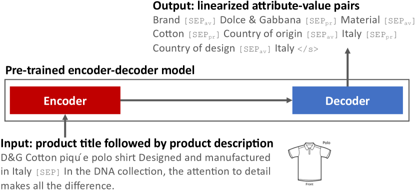
Figure 1: Overview of our generative approach for pavi; it takes product text to return a set of attribute-value pairs. In this example, the model generates Dolce & Gabbana as a brand, which is a canonicalized form of D&G, and two attributes have the entity Italy as values.

Unseen values.

Since values can be entities such as brands, models need to identify values unseen in the training data (Zheng et al., 2018). Since the classification-based approach assumes a pre-defined set of target classes (attribute-value pairs), it cannot handle such unseen attribute-value pairs.

Multi-attribute values.

When values can be associated with multiple attributes (e.g., Italy in Figure 1), models need to identify multiple attributes for a single value string in the text. To address this, the extraction-based approach must solve nested named entity recognition (Wang et al., 2020).

Canonicalized values.

E-commerce vendors need attribute values in the canonical form (e.g., Dolce & Gabbana for D&G) in actual services such as faceted product search Chen et al. (2022). The extraction-based approach needs a further step to canonicalize extracted raw value strings (Putthividhya and Hu, 2011; Zhang et al., 2021).

Approach	Unseen	Multi	Canon
Extraction	Support	Partially	Not
Classification	Not	Support	Support
Generation (ours)	Support	Support	Support

Table 1: Comparison of different pavi approaches in terms of the challenges: handling unseen values, multi-attribute values, and canonicalized values.

Motivated by the shortcomings of the existing approaches to pavi (Table 1), we propose to cast pavi as sequence-to-set generation, which can handle all the challenges by using canonicalized attribute-value pairs for training (Figure 1). We expect that 1) generation can decode unseen values by considering corresponding values in the input, 2) generation can decode the same string in the input multiple times as values for different attributes, and 3) generation can learn how to canonicalize raw strings in input. We finetune the pre-trained generative model t5 (Raffel et al., 2020) to autoregressively decode a set of attribute-value pairs from the given text. As discussed in (Vinyals et al., 2016; Yang et al., 2018; Madaan et al., 2022), the output order will matter to decode sets as a sequence. We therefore explore methods of composing an attribute-value pair and ordering the pairs for the task.

We evaluate our generative framework on two real-world datasets, mave (Yang et al., 2022) and our in-house product data. The experimental results demonstrate that our generation-based approach outperforms extraction- and classification-based methods on their target datasets.

Our contribution is as follows.

• We have solved the product attribute-value identification task as a sequence-to-set generation for the first time.

• We revealed the effective order of attribute-value pairs for the t5 model among various ordering schemes (Table 2).

• We provided the first comprehensive comparison among extraction-, classification-, and generation-based models on two real-world pavi datasets, and empirically confirmed that the generation-based models outperformed the others (Table 6) while addressing all challenges in pavi (Tables 9, 11 and 12).

2 Related Work

Product Attribute-Value Extraction

Traditionally, a myriad of previous studies formulated pavi as named entity recognition (ner) (Probst et al., 2007; Wong et al., 2008; Putthividhya and Hu, 2011; Bing et al., 2012; Shinzato and Sekine, 2013; More, 2016; Zheng et al., 2018; Rezk et al., 2019; Karamanolakis et al., 2020; Zhang et al., 2020). However, since the number of attributes in real-world e-commerce sites can exceed ten thousand (Xu et al., 2019), the ner-based models suffer from the data sparseness problem, which makes the models perform poorly. While the extraction-based approach can identify unseen values in the training data, it cannot canonicalize values by itself and is difficult to handle overlapping values, although nested ner (surveyed in Wang et al. (2022)) can remedy the latter issue.

Ordering	Attribute-value pairs placed in the target sequence
Rare-first	Material [sepav] Nylon [seppr] Color [sepav] Red [seppr] Color [sepav] White
Common-first	Color [sepav] White [seppr] Color [sepav] Red [seppr] Material [sepav] Nylon
Random	Color [sepav] Red [seppr] Material [sepav] Nylon [seppr] Color [sepav] White

Table 2: Example of attribute-value pair ordering with the attribute-then-value composition. We assume that the frequency of the pairs is $\langle$Color, White$\rangle>\langle$Color, Red$\rangle>\langle$Material, Nylon$\rangle$.

To mitigate the data sparseness problem, some studies leveraged qa models for the pavi task (Xu et al., 2019; Wang et al., 2020; Yang et al., 2022; Shinzato et al., 2022), by assuming the target attribute for extraction as additional input. These qa-based approaches take an attribute as query and product text as context, and extract attribute values from the context as answer for the query. Similar to the traditional ner-based models, these extractive qa-based models do not work for canonicalized values. To improve the ability to find unseen values, Roy et al. (2021) generated a value for the given product text and attribute. However, we need to apply these qa-based models to the same context with each of thousands of attributes, unless comprehensive attribute taxonomy is designed to narrow down possible attributes; such taxonomy is not always available and is often imperfect, as investigated by Mao et al. (2020) for Amazon.com.

Product Attribute-Value Identification as Classification

Chen et al. (2022) solved pavi as multi-label classification (mlc), assuming attribute-value pairs as target labels. One of the problems in this approach is that the distribution between positive and negative labels is heavily skewed because the number of possible attribute values per product is much smaller than the total number of attribute values. To alleviate the imbalanced label problem, they introduced a method called label masking to reduce the number of negative labels using an attribute taxonomy designed by the e-commerce platform. To mitigate the extreme multi-class classification, Fuchs and Acriche (2022) decomposed the target label, namely attribute-value pair, into two atomic labels, attribute and value, to perform a hierarchical classification. Although these classification-based approaches support canonicalized values and multi-attribute values, they cannot handle unseen values.

In this study, we adopt a generative approach to return a set of attribute-value pairs from given product data, and empirically compare it with the above two approaches. Our approach can be applied to the task settings adopted by the qa-based models, by simply feeding one (or more) target attributes as additional input (e.g., title [sep] description [sep] attributes) to decode their values in order.

3 Proposed Method

As mentioned above, previous studies formalize pavi as either sequence tagging or multi-label classification problems. These approaches do not address all the challenges derived from real-world e-commerce sites at the same time (Table 1).

We thus propose a unified generative framework that formalizes pavi as a sequence-to-set problem. Let us denote $\bm{x}=\{x_{1},x_{2},\ldots,x_{n}\}$ as product data (title and description) where $n$ is the number of tokens in $\bm{x}$. Given product data $\bm{x}$, the model is trained to return a set of attribute-value pairs $\bm{y}=\{\langle\bm{a_{1}},\bm{v_{1}}\rangle,\langle\bm{a_{2}},\bm{v_{2}}\rangle,\dots,\langle\bm{a_{k}},\bm{v_{k}}\rangle\}$ for $\bm{x}$, where $k$ is the number of attribute-value pairs associated with the product; $\bm{a}_{i}=\{a_{1},a_{2},\ldots,a_{m_{i}}\}$ and $\bm{v}_{i}=\{v_{1},v_{2},\ldots,v_{l_{i}}\}$ are corresponding attribute and value. $m_{i}$ and $l_{i}$ are the numbers of tokens in $\bm{a}_{i}$ and $\bm{v}_{i}$, respectively.

As the backbone of our approach, we employ t5 (Raffel et al., 2020), a pre-trained generative model based on Transformer (Vaswani et al., 2017) that maps an input sequence to an output sequence.

The key issue in formulating the pavi task as sequence-to-sequence generation is how to linearize a set of attribute-value pairs into a sequence. Firstly, we should consider how to associate attributes and their corresponding values in the output sequence. Secondly, the autoregressive generation decodes output tokens (here, attributes and values) one by one conditioned on the previous labels. Thus, if specific (or informative) tokens are first decoded, it will make it easy to decode the remaining tokens. However, due to the exposure bias, decoding specific (namely, infrequent) tokens are more likely to fail. To address the challenge, we decompose the issue on linearization into two subproblems on how to compose an attribute-value pair and how to order attribute-value pairs. In what follows, we will describe these subproblems.

	mave			In-House Product Data
	Train	Dev.	Test	Train	Dev.	Test
The number of examples	640,000	100,000	290,773	640,000	100,000	100,000
without values	150,412	23,220	67,936	0	0	0
The number of distinct attributes	693	660	685	1,320	1,119	1,123
The number of distinct attribute values	54,200	21,734	37,092	13,328	8,402	8,445
The number of distinct attribute-value pairs	63,715	25,675	43,605	14,829	9,310	9,356
The number of attribute-value pairs	1,594,855	249,543	722,130	2,966,227	463,463	462,507
with unseen values	0	4,667	13,578	0	443	491
with multi-attribute (or nested) values	134,290	20,832	60,832	103,727	16,280	15,843
whose values appear as raw strings in the product text	1,594,855	249,543	722,130	1,340,043	210,181	207,997
The average number of subwords per example (input)	253.73	253.73	253.56	357.87	359.89	356.93
The average number of subwords per example (output)	10.35	10.39	10.32	46.43	46.44	46.31
The average number of attributes per example	1.64	1.64	1.64	3.24	3.25	3.23
The average number of values per example	2.25	2.25	2.25	4.62	4.62	4.61
The average number of subwords per attribute	2.84	2.82	2.85	4.77	4.72	4.69
The average number of subwords per value	4.15	3.46	3.81	4.09	3.96	3.93

Table 3: Detailed statistics of the datasets. We used the t5 tokenizer to tokenize examples, attributes and values.

3.1 Composition of Attribute-Value Pair

We consider the following ways to compose an attribute-value pair. In both ways, attributes and values are separated by a special token [sep_av].

Attribute-then-value, $\langle$A, V$\rangle$

Attribute is placed, and then its value (e.g., Color [sep_av] White). In general, the vocabulary size of attributes is much smaller than that of values. Thus, models will be easier to decode attributes than values.

Value-then-attribute, $\langle$V, A$\rangle$

Value is placed, and then its attribute (e.g., White [sep_av] Color). This will be effective when the target values appear as raw strings in the given text and are easier to decode than attributes.

3.2 Ordering of Attribute-Value Pairs

In this work, we design three different types of the attribute-value pair ordering (Table 2). We use a special token [sep_pr] as a separator between pairs.

Rare-first

Specific attribute values (e.g., brands) can help models decode other attribute values. For example, since Levi’s has many products made of denim, it is easy to decode the material if Levi’s is decoded in advance. Meanwhile, since there are many brands that have products made of denim, decoding denim as a material in advance is useless to decode the brands. To capture this inter-value dependency, we assume a correlation between the frequency and specificity of attribute-value pairs, and place attribute-value pairs to the target sequence in rare-first ordering of attribute-value pair frequency calculated from the training data. The attribute-value pairs with the same ranking will be placed randomly for this and following ordering.

Common-first

When the model autoregressively decodes outputs, intermediate errors affect future decoding. Thus, it is important to decode from confident attribute-value pairs. Since models will be easier to decode attribute-value pairs that have more training examples, we place attribute-value pairs to the target sequence in the common-first ordering of attribute-value pair frequency. This approach is adopted by Yang et al. (2018) in solving multi-label document classification as generation.

Random

To see whether the orders matter, we randomly sort attribute-value pairs in the target sequence; more precisely, we collect, uniquify, and shuffle attribute-value pairs taken from all training examples, and sort the pairs in each example according to the obtained order of the pairs. If this random ordering shows inferior performance against the above orderings, we can conclude output orders matter in this task.

4 Experiments

We evaluate our generative approach to pavi using two real-world datasets. In the literature, different types of approaches are rarely compared due to the proprietary nature of codes and datasets in this task. We thus compare our generation-based model with extraction- and classification-based models, all of which are based on public pre-trained models, using not only in-house but also public datasets.

4.1 Datasets

We used mave (Yang et al., 2022) and our in-house product data for experiments. The mave dataset is designed to evaluate the extraction-based pavi models, while the in-house dataset is designed to evaluate classification-based models (Table 3).

Title	Description	(original attribute-value info.)	Attribute-value pairs
Chicago Blackhawks Pet Dog Hockey Jersey LARGE	Chicago Blackhawks pet jersey - size LARGE. This great-looking jersey features screened-on logos on the sleeves and screened-on team name/number on the back.	$\langle$ Type, Jersey, 0, 34, 40 $\rangle$, $\langle$ Type, jersey, 1, 23, 29 $\rangle$, $\langle$ Type, jersey, 1, 63, 69 $\rangle$, $\langle$ Clothing Type, Jersey, 0, 34, 40 $\rangle$, $\langle$ Clothing Type, jersey, 1, 23, 29 $\rangle$, $\langle$ Clothing Type, jersey, 1, 63, 69 $\rangle$, $\langle$ Special use, None $\rangle$	$\langle$ Type, Jersey $\rangle$, $\langle$ Type, jersey $\rangle$, $\langle$ Clothing Type, Jersey $\rangle$, $\langle$ Clothing Type, jersey $\rangle$, $\langle$ Special use, None $\rangle$
Northwave [northwave] Espresso Original Red Men’s / Women’s / Sneakers 25 - 27cm	Product description. These sneakers are the perfect accent for your feet and come in a soft red color. The sole is made of lightweight rubber to reduce weight. It is a popular color.	$\langle$ Shoe size (cm), 25.0 $\rangle$, $\langle$ Shoe size (cm), 26.0 $\rangle$, $\langle$ Shoe size (cm), 27.0 $\rangle$, $\langle$ Color, Red $\rangle$	$\langle$ Shoe size (cm), 25.0 $\rangle$, $\langle$ Shoe size (cm), 26.0 $\rangle$, $\langle$ Shoe size (cm), 27.0 $\rangle$, $\langle$ Color, Red $\rangle$

Table 4: Example product data in mave (top) and our in-house datasets (bottom, translated from Japanese), which include multi-attribute values (e.g., jersey) and non-canonicalized values (e.g., 25). mave provides tuples of an attribute, value, paragraph ID, and the value’s beginning and ending positions in the paragraph, while our in-house data provides canonicalized attribute values. To train bert-ner, values in text are annotated by using the value positions in mave and by matching with the canonicalized values in the in-house data. To train t5 and bert-mlc and evaluate all models, we use attribute-value pairs (right).

MAVE dataset compiles the product data taken from Amazon Review Data (Ni et al., 2019). The dataset contains various kinds of products such as shoes, clothing, watches, books, and home decor decals. Each example consists of product titles and descriptions, attribute, value, and span of the attribute value. To construct such tuples, Yang et al. (2022) trained five aveqa models (Wang et al., 2020) using a large amount of silver data where attribute values were annotated using manually tailored extraction rules. Then, they applied the trained models to the Amazon Review Data in order to detect spans of values corresponding to attributes given to the models. To produce attribute value spans with high precision, they chose only attribute values that all five models extracted (positive). In addition, if no span is extracted from either model, and there is no extracted span from the extraction rules, they consider that there are no values for the attributes (negative); refer to Table 4 for example product data. As a result, mave consists of 2,092,898 product data for training and 290,773 product data for testing. Similar to Yang et al. (2022), to make the training faster, we randomly selected 640,000 and 100,000 product data as the training and development sets from the original training data, respectively. We used the test data in mave for our evaluation as it is.

In-House Product Data is taken from our e-commerce platform, Rakuten, which sells a wide range of products such as smartphones, car supplies, furniture, clothing, and kitchenware. Each example consists of a tuple of title, description, and a set of attribute-value pairs. The sellers assign products attribute-value pairs defined in the attribute taxonomy provided by the e-commerce platform. Since both attributes and values in the taxonomy are canonicalized, there exist spelling gaps between values in the taxonomy and those in the product text (e.g., Dolce & Gabbana in the taxonomy and D&G in the title). For experiments, among our in-house product data with one or more attribute-value pairs, we randomly sampled 640,000, 100,000, and 100,000 product data for training, development, and testing, respectively.

	mave			In-House Product Data
	bert-ner	bert-mlc	t5	bert-ner	bert-mlc	bert-mlc w/ tax	t5
Training (10 epochs)	22	22	24 $\times$ 10	22	22	22	24 $\times$ 10
Inference (the dev set)	8	8	80 $\times$ 10	8	8	8	80 $\times$ 10
Inference (the test set)	1.6	1.6	16 $\times$ 6	0.8	0.8	0.8	8 $\times$ 6
Total	31.6	31.6	1,136	30.8	30.8	30.8	1,088

Table 5: GPU hours to perform our experiments. For t5, we finetune and evaluate *-first models for each composition (2 $\times$ 2 models). For the random ordering, we train three models for each composition (3 $\times$ 2 models), and check the performance on the development set to choose the model with the best micro F₁ for testing.

4.2 Models

We compare the following models:

BERT-NER: extraction-based model. On the top of bert, we place a classification layer that uses the outputs from the last layer of bert as feature representations of each subword. Each subword is classified into one of the labels. We employ bilou chunking scheme (Sekine et al., 1998; Ratinov and Roth, 2009); the total number of labels is $N\times 4+1$, where $N$ is the number of distinct attributes in the training data. We have used bert as the backbone here because the common extraction-based baseline (Zheng et al., 2018) uses classic BiLSTM-CRF as the backbone (Huang et al., 2015) and bert-based models outperform in qa-based models (Wang et al., 2020); bert-ner can be a stronger and easily replicable baseline.

To annotate entities in text, we referred the beginning and ending positions in tuples for mave, and performed a dictionary matching for our in-house dataset. If annotations are overlapped, we keep the longest token length value, and drop all other overlapping values. For multi-attribute values, we adopt the most frequent attribute-value pair.

BERT-MLC: classification-based model. We put a classification layer on the top of bert, and feed the embeddings of the cls token to the classification layer as a representation of given text (Chen et al., 2022). The model predicts all possible attribute values from the representation through the classification layer. The total number of labels is the number of attribute values in the training data.

BERT-MLC w/ Tax: the current state-of-the-art classification-based model that can be comparable with the other methods. We added to bert-mlc the label masking (Chen et al., 2022), which leverages the skewed distributions of attributes in training and testing, using an attribute taxonomy defined for our in-house data. Although this is the state-of-the-art classification-based method, it requires the attribute taxonomy as extra supervision. Since the mave dataset does not provide the attribute taxonomy, we train and evaluate this model only on our in-house dataset.

T5: generation-based model of ours. We finetune t5 on the training data obtained by each element in $\{$Attribute-then-value, Value-then-attribute$\}\times\{$Random, Rare-first, Common-first$\}$. For random ordering, we create three training data with different random seeds, next train a model on each training data, and then chose the model that achieves the best micro F₁ on the development set.

4.3 Implementations

			mave						In-House Product Data
Models			Micro			Macro			Micro			Macro
			P (%)	R (%)	F1	P (%)	R (%)	F1	P (%)	R (%)	F1	P (%)	R (%)	F1
extraction-based
bert-ner			96.38	84.91	90.28	80.36	57.75	64.61	96.09	40.26	56.75	45.26	18.12	23.50
classification-based
bert-mlc			93.52	70.37	80.31	40.53	20.72	25.40	94.53	74.43	83.29	40.81	18.05	22.82
bert-mlc w/ tax			-	-	-	-	-	-	93.65	77.47	84.79	58.19	32.76	39.33
generation-based (ours)
t5	$\langle$A, V$\rangle$	Rare-first	95.45	91.70	93.54	77.57	64.35	68.97	88.61	81.50	84.91	66.33	47.25	53.10
		Common-first	95.29	92.16	93.70	78.26	66.94	70.63	85.30	82.83	84.05	62.10	41.85	47.49
		Random	95.10	91.46	93.24	77.24	62.71	67.45	87.73	81.41	84.45	61.64	42.47	47.92
	$\langle$V, A$\rangle$	Rare-first	95.24	91.97	93.57	80.59	68.02	72.51	89.82	80.73	85.03	65.73	44.61	50.93
		Common-first	94.62	92.85	93.73	80.50	69.72	73.47	84.25	82.97	83.60	63.61	43.61	49.13
		Random	95.13	92.04	93.56	80.56	67.28	71.83	88.25	81.41	84.69	63.06	42.09	48.10

Table 6: Performance of each model on two pavi datasets; The best score is in bold face and the second best score is underlined. bert-mlc w/ tax uses the extra supervision (taxonomy) for label masking, and it reduces the size of labels relevant to inputs from 14,829 to 405 on average.

We implemented all models in PyTorch. We used t5-base and sonoisa/t5-base-japanese in Transformers (Wolf et al., 2020), both of which have 220M parameters, as the pre-trained t5 models for mave and our in-house data, respectively. For training and testing, we used the default hyperparameters provided with each model. We ran teacher forcing in training, and performed beam search of size four in testing. For bert-based models, we used bert-base-cased for mave, and cl-tohoku/bert-base-japanese for our in-house dataset, both of which have 110M parameters. We set 0.1 of a dropout rate to a classification layer.

We use Adam (Kingma and Ba, 2015) optimizer with learning rates shown in Table 14 in Appendix. We trained the models up to 10 epochs with a batch size of 32 and chose the models that perform the best micro F₁ on the development set.

Computing Infrastructure

We used NVIDIA DGX A100 GPU on a Linux (Ubuntu) server with a AMD EPYC 7742 CPU at 2.25 GHz with 2 TB main memory for performing the experiments. Table 5 shows GPU hours taken for the experiments.

4.4 Evaluation Measure

Following the literature Xu et al. (2019); Wang et al. (2020); Yang et al. (2022); Shinzato et al. (2022); Chen et al. (2022), we used micro and macro precision (P), recall (R), and F₁ as metrics. We compute macro performance in attribute-basis. Since the goal of pavi is not to detect spans of values in text but to assign attribute-value pairs to products, we pick one attribute-value pair from multiple identical attribute-value pairs in mave (e.g., $\langle$Type, jersey$\rangle$ in Table 4). Note that we do not need this unification process for our in-house dataset because it provides unique attribute-value pairs.

Since attribute values in the mave dataset are based on outputs from qa-based models (Wang et al., 2020) and those in our in-house data are assigned voluntarily by sellers on our marketplace, both datasets may contain some missing values. To reduce the impact of those missing attribute-value pairs, we discard predicted attribute-value pairs if there are no ground truth labels for the attributes.

In the mave dataset, there are attributes whose values do not appear in the text (negative). For the ground truth with such no attribute values, models can predict no values (NN), or incorrect values (FP_n) while for the ground truth with concrete attribute values, the model can predict no values (FN), correct values (TP), or incorrect values (FP_p). Based on those types of predicted values, P and R are computed as follows:

$$\text{P}=\frac{\lvert\text{TP}\rvert}{\lvert\text{TP}\rvert+\lvert\text{FP}_{\mathrm{p}}\rvert+\lvert\text{FP}_{\mathrm{n}}\rvert}\text{ , }\text{R}=\frac{\lvert\text{TP}\rvert}{\lvert\text{TP}\rvert+\lvert\text{FN}\rvert}.$$

F₁ is computed as $2\times\text{P}\times\text{R}$ / ($\text{P}+\text{R}$). Note that since there are no attributes with no values in our in-house dataset, the value of $|$FP${}_{\mathrm{n}}\rvert$ is always 0.

4.5 Results

Table 6 shows the performance of each model on mave and our in-house datasets. Our generation-based models with *-first ordering mostly outperformed the extraction- and classification-based baselines in terms of F₁. The differences between the best models and the baselines were significant ($p<0.0005$) under approximate randomized test (Noreen, 1989). The higher recall of our generation-based models suggests the impact of capturing inter-value dependencies (§ 3.2).

The impact of the composition of attribute-value pairs depends on whether the output values are canonicalized. On the mave dataset, the models with the value-then-attribute composition outperformed those with attribute-then-value composition in terms of macro F₁. This is because all output values appear in the mave dataset. Thus, to the models, it is easier to generate values than attributes. Meanwhile, the advantage of value-then-attribute composition is smaller on our in-house dataset since there is no guarantee that the target values appear in the text as raw strings.

The impact of the ordering of attribute-value pairs depends on the number of attribute-value pairs per example. On the in-house dataset, the models with rare-first ordering consistently outperformed those with common-first ordering in terms of F₁. This result implies that decoding specific attribute-value pairs in advance is more helpful to generate general attribute-value pairs on the in-house dataset. Meanwhile, there is no clear difference between the models with *-first orderings on the mave dataset, since the number of attribute-value pairs per example is small.

These results confirm that the generative approach learns to flexibly perform canonicalization if it is required in the training data. Meanwhile, the performance of extraction- and classification-based approaches depends on whether the attribute-value pairs are canonicalized or not.

	Models		# of distinct values (med: 19)
			(19, $\infty$)	(0, 19]	all
# training	hi	ner	90.5 / 80.1	90.2 / 69.3	90.5 / 77.3
examples		mlc	80.7 / 40.2	85.5 / 34.9	80.8 / 38.9
(med: 268)		t5	93.9 / 86.9	94.4 / 78.2	93.9 / 84.7
	lo	ner	77.0 / 71.6	72.0 / 41.7	74.6 / 50.3
		mlc	18.7 / 9.3	35.7 / 10.0	27.3 / 9.8
		t5	81.1 / 76.7	79.4 / 54.8	80.3 / 61.1
	all	ner	90.4 / 78.0	87.0 / 49.9	90.3 / 64.6
		mlc	80.4 / 32.6	78.4 / 17.4	80.3 / 25.4
		t5	93.8 / 84.4	91.7 / 61.7	93.7 / 73.5

Table 7: Micro / macro F₁ values of each approach on the mave dataset. ‘lo’ and ‘hi’ are intervals for the number of training examples, (0, 268] and (268, $\infty$], respectively. t5 refers to the common-first model with $\langle$V, A$\rangle$ composition, which achieves the best micro F₁.

Quantitative comparison of each approach

To see the detailed behaviors of individual approaches, we categorized the attributes in the mave and our in-house datasets according to the number of training examples and the number of distinct values per attribute. We divide the attributes into four according to median frequency and number of values.

Tables 7 and  8 list micro and macro F₁ values of each approach for each category of attributes on the mave and our in-house datasets, respectively. From the table, we can see that t5 shows the best performance in all categories. This suggests that t5 is more robust than bert-ner and bert-mlc in the pavi task. We can also observe that the performance of bert-mlc drops significantly for attributes with a small number of training examples compared to those with a large number of training examples; the classification-based approach makes an effort to better classify more frequent attributes. Meanwhile, the performance drops of bert-ner and t5 are more moderate than bert-mlc, especially on the mave dataset. Moreover, we can see that t5 shows better micro F₁ for attributes that have a smaller number of distinct values on our in-house dataset, whereas it shows better micro F₁ for attributes that have a larger number of distinct values on the mave dataset. This implies that, although it is easy for the generation-based approaches to extract diverse values from text, it is still difficult to canonicalize those diverse values.

4.6 Analysis

From the better macro F₁ of t5 with *-first ordering than with random ordering, we confirmed that our generation-based models successfully capture inter-value dependencies to decode attribute-value pairs. In what follows, we perform further analysis to see if the generative approach addresses the three challenges; namely, unseen, multi-attribute (or nested), and canonicalized values (Table 1).

Can generative models identify unseen values?

To see how effective our generative models are for unseen attribute values, we compare its performance with bert-ner on attribute-value pairs in the test data that do not appear in the training data (13,578 and 491 unseen values exist in the mave and in-house datasets, respectively).

	Models		# of distinct values (med: 3)
			(3, $\infty$)	(0, 3]	all
# training	hi	ner	56.4 / 29.6	62.9 / 31.6	56.8 / 30.2
examples		mlc	83.5 / 34.1	82.1 / 44.6	83.4 / 37.2
(med: 44)		t5	85.0 / 63.2	87.8 / 71.8	85.1 / 65.7
	lo	ner	25.2 / 14.8	27.7 / 14.0	26.8 / 14.3
		mlc	5.0 / 1.6	8.9 / 3.1	7.4 / 2.7
		t5	44.5 / 31.3	47.4 / 29.9	46.3 / 30.4
	all	ner	56.4 / 26.0	62.0 / 20.6	56.7 / 23.5
		mlc	83.5 / 26.3	80.6 / 18.8	83.3 / 22.8
		t5	84.9 / 55.5	86.8 / 45.7	85.0 / 50.9

Table 8: Micro / macro F₁ values of each approach on the in-house dataset. ‘lo’ and ‘hi’ are intervals for the number of training examples, (0, 44] and (44, $\infty$], respectively. t5 refers to the rare-first model with $\langle$V, A$\rangle$ composition, which achieves the best micro F₁.

Models			mave F1		In-House F1
			Micro	Macro	Micro	Macro
bert-ner			34.57	22.16	14.29	3.02
t5	$\langle$A, V$\rangle$	Rare-first	38.21	27.87	19.44	5.08
		Common-first	37.34	29.02	17.03	6.55
		Random	36.65	27.64	15.94	5.93
	$\langle$V, A$\rangle$	Rare-first	37.44	29.10	18.15	5.89
		Common-first	38.19	31.22	18.61	6.15
		Random	36.59	28.98	12.64	2.34

Table 9: Performance on unseen values. The scores of bert-mlc models are 0.

Table 9 shows the results. We can see that the t5 models outperform bert-ner, especially in terms of macro F₁. Although the extraction-based approach can extract unseen values, the unified generative approach works better for extracting unseen values than the extraction-based approach.

Required processing	Attribute-value pair	Text
Understand structured values	$\langle$Series, iPhone (Apple)$\rangle$	iPhone 6S iPhone Softbank…
	$\langle$Chest (cm), 104 - 112$\rangle$	…Size [L] Chest 110cm Length 66cm…
Refer to the world knowledge	$\langle$Sleeve length, Long$\rangle$	Women’s Trench Coat Dark Brown…
	$\langle$Indication, Rhinitis$\rangle$	For runny nose, nasal congestion, sore throat,…
Recognize paraphrase	$\langle$Material, Polyurethane$\rangle$	Material: PU leather / Plastic
	$\langle$Compatible brand, Galaxy S8 plus$\rangle$	SC-03J Galaxy S8$\mathit{+}$ Galaxy…
Understand text	$\langle$Feature, With card holder$\rangle$	The card slot is on the left.
	$\langle$With or without casters, With casters$\rangle$	Table leg: Pipe, twin-wheel casters with stopper…

Table 10: Example of canonicalization that t5 models need to perform to generate values that do not appear in text. Substrings in text that can be regarded as a clue to generate the values are in italic.

Models			mave F1		In-House F1
			Micro	Macro	Micro	Macro
bert-ner			47.85	35.60	81.35	45.54
bert-mlc			68.79	24.95	76.43	30.47
bert-mlc w/ tax			-	-	77.19	41.55
t5	$\langle$A, V$\rangle$	Rare-first	75.14	54.30	79.90	58.44
		Common-first	75.31	53.89	80.16	55.09
		Random	74.73	52.48	80.45	53.50
	$\langle$V, A$\rangle$	Rare-first	75.40	56.11	80.13	57.81
		Common-first	75.38	57.07	80.16	60.83
		Random	74.97	54.28	80.18	56.08

Table 11: Performance on attribute-value pairs that can be obtained only by identifying multi-attribute values.

Can generative models identify multi-attribute values?

Next, to see how effective our generative models are for identifying multi-attribute values, we compare its performance to the baselines on attribute-value pairs in the test data that appear only as multi-attribute (or nested) values in input text. The number of such values in the mave and our in-house datasets is 60,832 and 15,843, respectively.

Table 11 shows the results. We can see that the t5 models outperform all baselines in terms of macro F₁. Although the classification-based models can identify multi-attribute values, the generative models outperformed those models.

Can generative models identify canonicalized values?

Lastly, to verify how effective our generative models are for identifying canonicalized values, we compare its performance with bert-mlc (w/ tax) on 207,997 attribute-value pairs whose values do not appear as raw strings in the corresponding product text in our in-house dataset.

Table 12 shows the results. The t5 models show comparable performance to and outperform the baselines in terms of micro and macro F₁, respectively. To see what types of canonicalization the t5 models need to perform when the canonicalized values do not appear in the text, we manually inspect attribute-value pairs whose values do not appear in text on the development set.

Table 10 exemplifies canonicalization that t5 models need to perform. From the table, we can see that the canonicalization included understanding structure in values (labels) (e.g., iPhone is a product of Apple), referring the world knowledge (the coat has long sleeves), recognizing paraphrases (PU is an abbreviation of polyurethane), and understanding product descriptions (“the card slot is on the left” entails that the product has a card holder). We conclude that our generative model addressed all the challenges in the pavi task better than the other two approaches.

Models			Micro F1	Macro F1
bert-mlc			72.49	20.10
bert-mlc w/ tax			73.87	35.12
t5	$\langle$A, V$\rangle$	Rare-first	73.09	43.40
		Common-first	71.91	39.07
		Random	72.48	39.19
	$\langle$V, A$\rangle$	Rare-first	72.93	40.08
		Common-first	71.20	37.95
		Random	72.30	37.20

Table 12: Performance on attribute-value pairs whose values do not appear as raw strings in input text in our in-house test data. The score of bert-ner is 0.

5 Conclusions

We have proposed a generative framework for product attribute-value identification (pavi), which is a task to return a set of attribute-value pairs from product text on e-commerce sites. Our model can address the challenges of the pavi task; unseen values, multi-attribute values, and canonicalized values. We finetune a pre-trained model t5 to autoregressively decode a set of attribute-value pairs from the given product text. To linearize the set of attribute-value pairs, we explored two types of attribute-value composition and three types of the orderings of the attribute-value pairs. Experimental results on two real-world datasets demonstrated that our generative approach outperformed the extraction- and classification-based baselines.

We plan to augment the ability to decode unseen values by using a pluggable copy mechanism Liu et al. (2021). We will evaluate our model on another pavi setting where the target attribute(s) are given.

6 Limitations

Since our generative approach to product attribute-value identification autoregressively decodes a set of attribute-value pairs as a sequence, the inference is slow (Table 5) and how to linearize the set of attribute-value pairs in the training data will affect the performance (Table 6). The best way of composing an attribute-value pair and ordering the pairs will depend on the characteristics of the datasets such as the existence of canonicalized values and the number of attribute-value pairs per example. Those who attempt to apply our method to their own datasets should keep this in mind.

			mave						In-House Product Data
Models			Micro			Macro			Micro			Macro
			P (%)	R (%)	F1	P (%)	R (%)	F1	P (%)	R (%)	F1	P (%)	R (%)	F1
extraction-based (large)
bert-ner			96.85	86.65	91.47	79.85	61.76	67.71	96.33	40.26	56.79	46.57	18.60	24.23
classification-based (large)
bert-mlc			93.19	51.63	66.45	17.31	7.40	9.49	NaN	0	NaN	NaN	0	NaN
bert-mlc w/ tax			-	-	-	-	-	-	94.36	77.99	85.40	52.36	28.01	33.92
generation-based (ours)
t5	$\langle$A, V$\rangle$	Rare-first	95.45	91.70	93.54	77.57	64.35	68.97	88.61	81.50	84.91	66.33	47.25	53.10
		Common-first	95.29	92.16	93.70	78.26	66.94	70.63	85.30	82.83	84.05	62.10	41.85	47.49
		Random	95.10	91.46	93.24	77.24	62.71	67.45	87.73	81.41	84.45	61.64	42.47	47.92
	$\langle$V, A$\rangle$	Rare-first	95.24	91.97	93.57	80.59	68.02	72.51	89.82	80.73	85.03	65.73	44.61	50.93
		Common-first	94.62	92.85	93.73	80.50	69.72	73.47	84.25	82.97	83.60	63.61	43.61	49.13
		Random	95.13	92.04	93.56	80.56	67.28	71.83	88.25	81.41	84.69	63.06	42.09	48.10

Table 13: Performance of each model on two pavi datasets. We used bert_large as a base model for extraction- and classification-based approaches. The best score is in bold face and the second best score is underlined. bert-mlc w/ tax uses the extra supervision (taxonomy) for label masking, and it reduces the size of labels relevant to inputs from 14,829 to 405 on average.

Hyperparameters	bert-ner	bert-mlc	t5
Max token length (encoder)	512	512	512
Max token length (decoder)	n/a	n/a	256
Epoch	10	10	10
Batch size	32	32	32
Dropout rate (classifier)	0.1	0.1	n/a
Learning rate	5e-5	5e-5	3e-4
Weight decay	0	0	0

Table 14: Hyperparameters for training models.

Appendix A Final Hyperparameters Used for Each Model

Table 14 shows the hyperparameters we used for training models. Other than those, we follow the default hyperparameters of t5  and bert  available from the HuggingFace models.

Appendix B Performance of Models Using bert_large

Table 13 shows the performance of models when we use bert_large as the base model for extraction- and classification-based approaches. We adopt bert-large-cased for mave and cl-tohoku/bert-large-japanese for our in-house data. From the table, we can see that training bert-mlc did not work well on both datasets. Especially, we cannot compute the performance on our in-house data because the model did not predict any attribute-value pairs for all inputs. Although bert_large has a larger number of parameters (330M) than the t5 models (220M), bert-ner based on bert_large still shows lower performance than our generative models on both datasets. This result means that our generative approach is more effective in the pavi task than the extraction-based approaches based on bert-ner. Meanwhile, bert-mlc w/ tax shows a slightly better micro F₁ score than ours. Given that it requires an attribute taxonomy as the extra supervision and exhibits low macro F₁, the generative approach is sufficiently comparable to the classification-based approach.

References

- Bing et al. (2012) Lidong Bing, Tak-Lam Wong, and Wai Lam. 2012. Unsupervised extraction of popular product attributes from web sites. In Information Retrieval Technology, pages 437–446, Berlin, Heidelberg. Springer Berlin Heidelberg.
- Chen et al. (2022) Wei-Te Chen, Yandi Xia, and Keiji Shinzato. 2022. Extreme multi-label classification with label masking for product attribute value extraction. In Proceedings of The Fifth Workshop on e-Commerce and NLP (ECNLP 5), pages 134–140, Dublin, Ireland. Association for Computational Linguistics.
- Fuchs and Acriche (2022) Gilad Fuchs and Yoni Acriche. 2022. Product titles-to-attributes as a text-to-text task. In Proceedings of The Fifth Workshop on e-Commerce and NLP (ECNLP 5), pages 91–98, Dublin, Ireland. Association for Computational Linguistics.
- Huang et al. (2015) Zhiheng Huang, Wei Xu, and Kai Yu. 2015. Bidirectional LSTM-CRF models for sequence tagging. CoRR, arXiv:1508.01991.
- Karamanolakis et al. (2020) Giannis Karamanolakis, Jun Ma, and Xin Luna Dong. 2020. TXtract: Taxonomy-aware knowledge extraction for thousands of product categories. In Proceedings of the 58th Annual Meeting of the Association for Computational Linguistics, pages 8489–8502, Online. Association for Computational Linguistics.
- Kingma and Ba (2015) Diederik P. Kingma and Jimmy Ba. 2015. Adam: A method for stochastic optimization. In Proceedings of the third International Conference on Learning Representations, San Diego, CA, USA.
- Liu et al. (2021) Yi Liu, Guoan Zhang, Puning Yu, Jianlin Su, and Shengfeng Pan. 2021. BioCopy: A plug-and-play span copy mechanism in Seq2Seq models. In Proceedings of the Second Workshop on Simple and Efficient Natural Language Processing, pages 53–57, Virtual. Association for Computational Linguistics.
- Madaan et al. (2022) Aman Madaan, Dheeraj Rajagopal, Niket Tandon, Yiming Yang, and Antoine Bosselut. 2022. Conditional set generation using seq2seq models. In Proceedings of the 2022 Conference on Empirical Methods in Natural Language Processing, pages 4874–4896, Abu Dhabi, United Arab Emirates. Association for Computational Linguistics.
- Mao et al. (2020) Yuning Mao, Tong Zhao, Andrey Kan, Chenwei Zhang, Xin Luna Dong, Christos Faloutsos, and Jiawei Han. 2020. Octet: Online catalog taxonomy enrichment with self-supervision. In Proceedings of the 26th ACM SIGKDD International Conference on Knowledge Discovery & Data Mining, KDD ’20, page 2247–2257, New York, NY, USA. Association for Computing Machinery.
- More (2016) Ajinkya More. 2016. Attribute extraction from product titles in ecommerce. In KDD 2016 Workshop on Enterprise Intelligence, San Francisco, CA, USA.
- Ni et al. (2019) Jianmo Ni, Jiacheng Li, and Julian McAuley. 2019. Justifying recommendations using distantly-labeled reviews and fine-grained aspects. In Proceedings of the 2019 Conference on Empirical Methods in Natural Language Processing and the 9th International Joint Conference on Natural Language Processing (EMNLP-IJCNLP), pages 188–197, Hong Kong, China. Association for Computational Linguistics.
- Noreen (1989) Eric W. Noreen. 1989. Computer-intensive methods for testing hypotheses. Wiley, New York.
- Probst et al. (2007) Katharina Probst, Rayid Ghani, Marko Krema, Andrew E. Fano, and Yan Liu. 2007. Semi-supervised learning of attribute-value pairs from product descriptions. In Proceedings of the 20th International Joint Conference on Artificial Intelligence, IJCAI’07, pages 2838–2843, Hyderabad, India. Morgan Kaufmann Publishers Inc.
- Putthividhya and Hu (2011) Duangmanee Putthividhya and Junling Hu. 2011. Bootstrapped named entity recognition for product attribute extraction. In Proceedings of the 2011 Conference on Empirical Methods in Natural Language Processing, pages 1557–1567, Edinburgh, Scotland, UK. Association for Computational Linguistics.
- Raffel et al. (2020) Colin Raffel, Noam Shazeer, Adam Roberts, Katherine Lee, Sharan Narang, Michael Matena, Yanqi Zhou, Wei Li, and Peter J. Liu. 2020. Exploring the limits of transfer learning with a unified text-to-text transformer. J. Mach. Learn. Res., 21(140):1–67.
- Ratinov and Roth (2009) Lev Ratinov and Dan Roth. 2009. Design challenges and misconceptions in named entity recognition. In Proceedings of the Thirteenth Conference on Computational Natural Language Learning (CoNLL-2009), pages 147–155, Boulder, Colorado. Association for Computational Linguistics.
- Rezk et al. (2019) Martin Rezk, Laura Alonso Alemany, Lasguido Nio, and Ted Zhang. 2019. Accurate product attribute extraction on the field. In Proceedings of the 35th IEEE International Conference on Data Engineering, pages 1862–1873, Macau SAR, China. IEEE.
- Roy et al. (2021) Kalyani Roy, Pawan Goyal, and Manish Pandey. 2021. Attribute value generation from product title using language models. In Proceedings of The 4th Workshop on e-Commerce and NLP, pages 13–17, Online. Association for Computational Linguistics.
- Sekine et al. (1998) Satoshi Sekine, Ralph Grishman, and Hiroyuki Shinnou. 1998. A decision tree method for finding and classifying names in Japanese texts. In Sixth Workshop on Very Large Corpora, pages 171–178, Quebec, Canada.
- Shinzato and Sekine (2013) Keiji Shinzato and Satoshi Sekine. 2013. Unsupervised extraction of attributes and their values from product description. In Proceedings of the Sixth International Joint Conference on Natural Language Processing, pages 1339–1347, Nagoya, Japan. Asian Federation of Natural Language Processing.
- Shinzato et al. (2022) Keiji Shinzato, Naoki Yoshinaga, Yandi Xia, and Wei-Te Chen. 2022. Simple and effective knowledge-driven query expansion for QA-based product attribute extraction. In Proceedings of the 60th Annual Meeting of the Association for Computational Linguistics (Volume 2: Short Papers), pages 227–234, Dublin, Ireland. Association for Computational Linguistics.
- Vaswani et al. (2017) Ashish Vaswani, Noam Shazeer, Niki Parmar, Jakob Uszkoreit, Llion Jones, Aidan N Gomez, Łukasz Kaiser, and Illia Polosukhin. 2017. Attention is all you need. In Advances in Neural Information Processing Systems, volume 30, pages 5998–6008, Red Hook, NY, USA. Curran Associates, Inc.
- Vinyals et al. (2016) Oriol Vinyals, Samy Bengio, and Manjunath Kudlur. 2016. Order matters: Sequence to sequence for sets. In The fourth International Conference on Learning Representations, San Juan, Puerto Rico.
- Wang et al. (2020) Qifan Wang, Li Yang, Bhargav Kanagal, Sumit Sanghai, D. Sivakumar, Bin Shu, Zac Yu, and Jon Elsas. 2020. Learning to extract attribute value from product via question answering: A multi-task approach. In Proceedings of the 26th ACM SIGKDD International Conference on Knowledge Discovery and Data Mining, KDD ’20, pages 47–55, New York, NY, USA. Association for Computing Machinery.
- Wang et al. (2022) Yu Wang, Hanghang Tong, Ziye Zhu, and Yun Li. 2022. Nested named entity recognition: A survey. ACM Trans. Knowl. Discov. Data, 16(6):1–29.
- Wolf et al. (2020) Thomas Wolf, Lysandre Debut, Victor Sanh, Julien Chaumond, Clement Delangue, Anthony Moi, Pierric Cistac, Tim Rault, Remi Louf, Morgan Funtowicz, Joe Davison, Sam Shleifer, Patrick von Platen, Clara Ma, Yacine Jernite, Julien Plu, Canwen Xu, Teven Le Scao, Sylvain Gugger, Mariama Drame, Quentin Lhoest, and Alexander Rush. 2020. Transformers: State-of-the-art natural language processing. In Proceedings of the 2020 Conference on Empirical Methods in Natural Language Processing, pages 38–45, Online. Association for Computational Linguistics.
- Wong et al. (2008) Tak-Lam Wong, Wai Lam, and Tik-Shun Wong. 2008. An unsupervised framework for extracting and normalizing product attributes from multiple web sites. In Proceedings of the 31st Annual International ACM SIGIR Conference on Research and Development in Information Retrieval, SIGIR ’08, page 35–42, New York, NY, USA. Association for Computing Machinery.
- Xu et al. (2019) Huimin Xu, Wenting Wang, Xin Mao, Xinyu Jiang, and Man Lan. 2019. Scaling up open tagging from tens to thousands: Comprehension empowered attribute value extraction from product title. In Proceedings of the 57th Annual Meeting of the Association for Computational Linguistics, pages 5214–5223, Florence, Italy. Association for Computational Linguistics.
- Yang et al. (2022) Li Yang, Qifan Wang, Zac Yu, Anand Kulkarni, Sumit Sanghai, Bin Shu, Jon Elsas, and Bhargav Kanagal. 2022. MAVE: A product dataset for multi-source attribute value extraction. In Proceedings of the Fifteenth ACM International Conference on Web Search and Data Mining, WSDM ’22, page 1256–1265, New York, NY, USA. Association for Computing Machinery.
- Yang et al. (2018) Pengcheng Yang, Xu Sun, Wei Li, Shuming Ma, Wei Wu, and Houfeng Wang. 2018. SGM: Sequence generation model for multi-label classification. In Proceedings of the 27th International Conference on Computational Linguistics, pages 3915–3926, Santa Fe, New Mexico, USA. Association for Computational Linguistics.
- Zhang et al. (2021) Danqing Zhang, Zheng Li, Tianyu Cao, Chen Luo, Tony Wu, Hanqing Lu, Yiwei Song, Bing Yin, Tuo Zhao, and Qiang Yang. 2021. QUEACO: Borrowing treasures from weakly-labeled behavior data for query attribute value extraction. In Proceedings of the 30th ACM International Conference on Information and Knowledge Management, CIKM ’21, page 4362–4372, New York, NY, USA. Association for Computing Machinery.
- Zhang et al. (2020) Hanchu Zhang, Leonhard Hennig, Christoph Alt, Changjian Hu, Yao Meng, and Chao Wang. 2020. Bootstrapping named entity recognition in E-commerce with positive unlabeled learning. In Proceedings of The 3rd Workshop on e-Commerce and NLP, pages 1–6, Seattle, WA, USA. Association for Computational Linguistics.
- Zheng et al. (2018) Guineng Zheng, Subhabrata Mukherjee, Xin Luna Dong, and Feifei Li. 2018. OpenTag: Open attribute value extraction from product profiles. In Proceedings of the 24th ACM SIGKDD International Conference on Knowledge Discovery and Data Mining, KDD ’18, pages 1049–1058, New York, NY, USA. Association for Computing Machinery.