Operator growth and Krylov Complexity in Bose-Hubbard Model

Abstract

We study Krylov complexity of a one-dimensional Bosonic system, the celebrated Bose-Hubbard Model. The Bose-Hubbard Hamiltonian consists of interacting bosons on a lattice, describing ultra-cold atoms. Apart from showing superfluid-Mott insulator phase transition, the model also exhibits both chaotic and integrable (mixed) dynamics depending on the value of the interaction parameter. We focus on the three-site Bose Hubbard Model (with different particle numbers), which is known to be highly mixed. We use the Lanczos algorithm to find the Lanczos coefficients and the Krylov basis. The orthonormal Krylov basis captures the operator growth for a system with a given Hamiltonian. However, the Lanczos algorithm needs to be modified for our case due to the instabilities instilled by the piling up of computational errors. Next, we compute the Krylov complexity and its early and late-time behaviour. Our results capture the chaotic and integrable nature of the system. Our paper takes the first step to use the Lanczos algorithm non-perturbatively for a discrete quartic bosonic Hamiltonian without depending on the auto-correlation method.

1 Introduction

Quantum mechanics is a staple ingredient in the playground of every theoretical physicist and is also responsible for most modern developments in natural sciences. A basic idea during our introductory lessons in quantum mechanics is the evolution of a simple operator $\mathcal{O}$ with time $t$ for a system governed by a Hamiltonian $H$. In the Heisenberg picture, the simple operator $\mathcal{O}$ at $t=0$ grows in the Hilbert Space into a complex operator $\mathcal{O}(t)$ through $e^{iHt}\mathcal{O}e^{iHt}$. This growth quantifies the spread of local information supported by a single or small number of sites to the entire system. The nature of the operator growth depends on the system’s Hamiltonian. An operator, for example, will grow into an integrable and non-integrable system in distinct ways. Using the Baker-Campbell-Hausdorff formula, the operator growth is expressed in terms of complicated nested commutators $[H,[H,\cdots[H,\mathcal{O}]]]$. We soon realize that the evaluation becomes rapidly difficult to perform with each level of the nested commutator. Nevertheless, this simple notion of operator growth plays a massive role in diverse areas of physics. The ‘dissipative’ behaviour of the operator growth is recently found to be connected to the thermalization of a given system vonKeyserlingk:2017dyr ; Nahum:2017yvy ; Khemani:2017nda ; Rakovszky:2017qit ; Gopalakrishnan:2018wyg .

Another common way of describing the operator growth in the space-time picture is by the out-of-time-ordered (OTOC) commutator 1969JETP…28.1200L ; Xu:2018dfp ; Nahum:2017yvy ; vonKeyserlingk:2017dyr ; Gu:2021xaj . The classical chaos makes the OTOC grow exponentially, also known as the Lyapunov exponent. The interesting conjecture is that the Lyapunov exponent is bounded from above Maldacena:2015waa for a few strongly coupled large-N models (the Sachdev-Ye-Kitaev (SYK) model, for example, having a dual in the gravity side) Maldacena:2016hyu ; Kitaev15 ; PhysRevLett.70.3339 . However, the bound on the Lyapunov exponent is not seen universally, especially for generic, non-integrable Hamiltonians outside of the semi-classical, large-N limit Khemani:2017nda ; PhysRevE.89.012923 ; Xu:2018xfz ; Xu:2018dfp .

A general theory of operator growth under generic, non-integrable Hamiltonian dynamics is recently given by Parker et al Parker:2018yvk . The authors argued that, with each increasing level of the nested commutators in the operator growth, the growing operators increase exponentially in time. The exponential size of the computation enables the system to be essentially treated as a thermodynamic entity, thus, emerging a statistical picture. This gave rise to the idea of governing the operator growth with some universal properties, even for non-integrable systems in arbitrary dimensions. The hypothesis for universal operator growth in Parker:2018yvk is based on the notion of a recursive technique, the Lanczos algorithm. Starting with a test operator $|\mathcal{O}(t=0))$, the Lanczos algorithm iteratively generates a set of orthonormal basis operators. This basis of orthonormal operators is called the Krylov basis $|\mathcal{O}_{n})$, which can have fewer elements than the dimension of the Hilbert space, depending on the dynamics and the choice of the initial operator. Along with the basis operators $|\mathcal{O}_{n})$ (where $n=0,1,\cdots,$ denotes the dimension of Krylov space), a set of coefficients $\{b_{n}\}$ is generated, known as Lanczos coefficients. The time evolved operator $|\mathcal{O}(t))$ is expanded in terms of the Krylov basis $|\mathcal{O}_{n})$ and time-dependent coefficients $\phi_{n}(t)$, which obeys discrete Schrödinger equations Parker:2018yvk . The operator dynamics is encoded in these time-dependent coefficients, which can also be thought of as wavefunctions distributed over the Krylov basis. The operator growth can be understood as the delocalization of an initial operator which we choose to be $|\mathcal{O}_{0})$ over the Kyrlov basis with time, and the hopping amplitudes are given by the Lanczos coefficients.

The concept of various notions of complexity follows naturally from the above observation. For example, Parker et.al Parker:2018yvk have introduced the notion of Krylov complexity, ( or K-complexity) as a measure of quantum chaos in the thermodynamic limit, that depends on the local Hamiltonian, a specific choice of an inner product, and the choice of the reference operator. K-Complexity of a generic operator in a finite-dimensional system size exhibits a specific profile with time which was first shown in Barbon:2019wsy and then in Rabinovici:2020ryf . With an aim to find the chaotic nature of the system, we perform a numerical analysis to find the profile of K-Complexity at all time scales, including the scrambling phase and the late time phase, and compare our results to those of Barbon:2019wsy ; Rabinovici:2020ryf .

The Lanczos coefficients ${b_{n}}$, in a quantum chaotic system, are hypothesized to grow fast. The maximum possible growth varies linearly with $n$ Parker:2018yvk , modified by a logarithmic correction in local $(1+1$)-dimensional lattice systems. This is in contrast, to the integrable models, Barbon:2019wsy where the Lanczos coefficients grow as $b_{n}\sim\alpha n^{\delta}$, where $0<\delta<1$. This behaviour of the Lanczos coefficients $b_{n}$, implies that the K-complexity grows exponentially in time in chaotic systems and powerlike in an integrable system. In recent times this has motivated lots of studies. Interested readers are referred to some of these references, which are by no means exhaustive Barbon:2019wsy ; Jian:2020qpp ; DymarskyPRB2020 ; PhysRevLett.124.206803 ; Yates2020 ; Rabinovici:2020ryf ; Rabinovici:2021qqt ; Yates:2021lrt ; Yates:2021asz ; Dymarsky:2021bjq ; Noh2021 ; Trigueros:2021rwj ; https://doi.org/10.48550/arxiv.2207.13603 ; Fan_2022 ; Kar_2022 ; https://doi.org/10.48550/arxiv.2109.03824 ; PhysRevE.106.014152 ; https://doi.org/10.48550/arxiv.2204.02250 ; Bhattacharjee_2022 ; Bhattacharjee_2022a ; Du:2022ocp ; Banerjee:2022ime ; https://doi.org/10.48550/arxiv.2205.12815 ; https://doi.org/10.48550/arxiv.2207.05347 ; H_rnedal_2022 ; https://doi.org/10.48550/arxiv.2208.13362 ; Bhattacharjee:2022lzy ; Rabinovici:2022beu ; Alishahiha:2022anw ; Avdoshkin:2022xuw ; Kundu:2023hbk ; Rabinovici:2023yex ; Zhang:2023wtr ; Nizami:2023dkf ; Hashimoto:2023swv ; Nandy:2023brt ; Balasubramanian:2022tpr ; Balasubramanian:2021mxo ; Caputa2022PRB ; Caputa:2022yju ; https://doi.org/10.48550/arxiv.2208.10520 ; Erdmenger:2023shk ; Bhattacharya:2023zqt ; Chattopadhyay:2023fob ; Pal:2023yik .

Motivated by all these, we have initiated a study of operator growth for the Bose-Hubbard model in this paper. It has found important application in the field of ultracold atom physics jaksch1998cold . This model exhibits Superfluidity-Mott insulator phase transition sachdev1999quantum , which has been observed experimentally with ultracold atoms in optical lattice Sengupta:2005 . More importantly, this model provides us with a rich parameter space, tuning by which it can behave as chaotic or non-chaotic (integrable) systems PhysRevA.74.033601 ; Viscondi_2011 ; PhysRevA.101.053604 . Although for the system with fewer degrees of freedom, this kind of mixed behaviour can be expected FEINGOLD1983433 ; PhysRevA.30.509 ; PhysRevA.35.1464 , but for a generic quantum many-body system mixed systems are less common Nakerst:2022prc . So this model provides us with an ideal playground to study operator growth as well as the associated Krylov complexity for both the chaotic and integrable regime and make a comparison. In Nakerst:2022prc , the authors have considered a classical limit by parametrizing the interaction by $\beta=U\,N$, where $U$ is the on-site interaction and the particle number is $N$, and then showed that in the limits $\beta\rightarrow 0$ and $\beta\rightarrow\infty$, the three-site Bose-Hubbard model possess integrable nature due to the vanishing of the only positive Lyapunov exponent $\lambda_{\text{max}}.$ Also, this model presents us with an excellent opportunity to study the operator growth and the Krylov complexity for a quantum-many body system consisting of bosonic degrees of freedom system containing quartic interaction terms using the Lanczos algorithm non-perturbatively. To the best of our knowledge, in the past, only limited studies of this kind have been made for non-quadratic systems .

The paper is organized as follows. In Sec. 2, we introduce the necessary details of the celebrated Bose-Hubbard model, used in the context of our current analysis. In Sec. 4, we dive into the details of the Krylov basis and spanning of the Krylov space, which is significantly different from the Hilbert space. Then, in Sec. 5, we revisit the Lanczos algorithm. Even after being a powerful technique, Lanczos method suffers terribly from instabilities and errors rounding up in the process. This lead to this Sec. 5, where we discuss the resolution to apply the modified version of the Lanczos method. Our results of the operator growth for the Bose-Hubbard model is presented in Sec. 6 and that of the Krylov complexity is presented in Sec. 7. Finally we end with a summary of our results and future directions in Sec. 8. We also have incorporated Appendices (A), (B) and (C) explaining more details of our numerical analysis.

2 Bose-Hubbard model

In this section, we start by summarising the necessary details of the one-dimensional Bose-Hubbard model. The Bose-Hubbard model consists of interacting bosons placed on a lattice. The model rose to prominence to describe the dynamics of ultracold bosonic atoms in an optical lattice, with the system parameters being completely controllable by laser light jaksch1998cold . We restrict the model to open-boundary chains of length $M$ with a vanishing chemical potential. The Hamiltonian is given by

$$H=-J\sum_{<i,j>}^{M-1}(a_{i}^{{\dagger}}a_{j}+a_{j}^{{\dagger}}a_{i})+\frac{U}{2}\sum_{i=1}^{M}\hat{n}_{i}(\hat{n}_{i}-1)$$ (1)

where $<i,j>\equiv<j,i>$ denotes the summation over adjacent sites $(j=i\pm 1)$, $a_{i}^{{\dagger}}$ and $a_{i}$ are the bosonic creation and annihilation operators on the site $i$ (with the site $i$ running from 1 to the site number). Also, $\hat{n}_{i}=a_{i}^{{\dagger}}a_{i}$ is the number operator that counts the number of particles on that site $i$. Here, $M$ denotes the site number, and $N$ is the particle number. In the first term, the summation runs up to $M-1$ when we consider the fixed boundary condition, such that particles are to be arranged in a linear chain with non-interacting walls at the end. Another possible boundary condition is to put the particles in a circle with the $M+1$-th site being identified as the first site. In this periodic boundary condition, the summation over the first term runs up to $M$. $J$ is the tunnelling coefficient which signifies the energy gained due to the particles hopping from one site to its neighbouring site. In this paper, we will only use open boundary condition. The first term proportional to $J$ is the kinetic term of the Hamiltonian. On the other hand, the parameter $U$ characterizes the two-particle on-site repulsive interaction strength. A point of importance is that the parameters $J$ and $U$ can be adjusted by various means. The model with a finite value of chemical potential shows two different phases depending on the ratio of the two parameters $\Lambda\equiv\frac{U}{J}$ measured in terms of the energies. For $\Lambda<<1$, the phase is identified by weak coupling and strong hopping, giving rise to the super-fluid phase. Additionally, $\Lambda>>1$ with strong coupling and weak hopping characterizes the Mott-insulator phase Marvin .

The Hamiltonian has a $U(1)$ symmetry associated with the conservation of a total number of particles. The symmetry group of the open boundary Hamiltonian can therefore be written as a $U(1)$. For closed boundary conditions, the symmetry group of the Hamiltonian becomes $U(1)\otimes D_{M}$, where the symmetry $D_{M}$ is the combination of translation and reflection symmetries. The dimension of the Hilbert space $\mathcal{H}$ with the total number of atom $N$ and number of sites $M$ is found to be

$$D=\frac{(N+M-1)!}{N!(M-1)!}\,.$$ (2)

The dimension $D$ grows with the number of particles $N$ as $D\sim N^{M+1}$ for a fixed $M$. A classical limit exists in the Bose-Hubbard model when the particle number $N\to\infty$ with the site number $M$ is kept fixed. The classical limit is similar to the discreet non-linear Schrodinger equation. The interaction is usually parametrized in the classical limit by $\mathfrak{\beta}=UN$. The model in the $\beta=0$ and $\beta=\infty$ limits are integrable, thus, analytically solvable. For the site number $M=2$, the model is solvable for all values of $\beta$. Otherwise, for $M\geq 3$ and finite $\beta$, the Bose-Hubbard model is non-integrable Nakerst:2022prc . However, for $M=3$, the model shows neither strongly chaotic nor integrable behaviour. It is said to exhibit highly mixed behaviour. Our findings in Sec 6, also confirm the said behaviour. In the following sections, we analyze the Bose-Hubbard model for site number $M=3$ with different values of the particle number $N$ and $\Lambda\equiv\frac{U}{J}$. It is possible to generalize our results for higher particle and site numbers. However, the computations grow excessively expensive and are thus limited by the computational power. We will study the time evolution of an operator with a fixed Hamiltonian Eq.(1) in Krylov space. We use the Lanczos algorithm to find the appropriate Krylov basis and the corresponding Lanczos coefficients. To the best of our understanding, this is the first time the Lanczos algorithm (appropriately modified, discussed in later sections) is being used for a bosonic lattice system.

3 Revisiting the Krylov Space

In this section, we review the details of the Krylov Basis and its relation to the Krylov space. The Krylov basis is an ordered, orthonormal set of base kets that contains information about the time evolution of an operator. We begin by choosing an appropriate basis associated with the Hilbert space $\mathcal{H}$ with dimension $dim(\mathcal{H})=D$. The associated Hilbert space of linear operators $L(\mathcal{H})\equiv\hat{\mathcal{H}}$ that acts on $\mathcal{H}$, is of dimension $D^{2}$. Next, we choose a system of $N$ particles in $M$ sites governed by the Hamiltonian ($H$) defined in Eq.(1) and an operator $\mathcal{O}$ ($H,\mathcal{O}\in\hat{\mathcal{H}}$) Rabinovici:2020ryf . A natural choice of basis for the Bose-Hubbard Hamiltonian is the base ket with the occupation numbers in each site, i.e. $\ket{{n_{1},n_{2},\cdots,n_{M}}}$, which are eigenstates of number operators $\hat{n_{i}}$

$$\hat{n_{i}}\,\ket{{n_{1},n_{2},\cdots,n_{M}}}=n_{i}\,\ket{{n_{1},n_{2},\cdots,n_{M}}}.$$ (3)

Here, $n_{i}\geq 0$ and $\sum_{i=1}^{N}\,n_{i}=N$. One can construct all the basis vectors with appropriate $N$, and $M$ following the rules mentioned in Zhang_2010 .

Next, we choose an initial operator $\mathcal{O}\in\hat{\mathcal{H}}$ and evolve it in time. The operator $\mathcal{O}$ gradually explores a subspace of the space of operators of the given system during its evolution. This subspace is called the Krylov space. The orthonormal Krylov basis $\mathcal{K}$ and the structure of the Krylov space can be analyzed using the powerful algorithm known as the Lanczos algorithm Parker:2018yvk . The Lanczos algorithm also captures the rate at which a typical operator span the Krylov space. The Krylov basis $\mathcal{K}$ depends on the choice of the initial operator, and the dynamics of the system may not expand the entire Hilbert space $\mathcal{H}$. We use the smooth-ket notation $|\mathcal{O})$ to denote the element of the operator space corresponding to an operator $\mathcal{O}$ throughout the paper. In the following paragraph, we explain the notions of the Krylov Basis and Krylov space in the context of an operator growth $\mathcal{O}(t)$.

In the Heisenberg picture, the time evolution of $|\mathcal{O})$ is given by

$$\Big{|}\mathcal{O}(t)\Big{)}=e^{iHt}|\mathcal{O})e^{-iHt}=e^{i\mathcal{L}t}|\mathcal{O}).$$ (4)

Here, $\mathcal{L}$ is the Liouvillian operator defined by $\mathcal{L}|\mathcal{O})=\Big{|}[H,\mathcal{O}]\Big{)}$ with $H$ being the system Hamiltonian Eq.(1). Thus, using the Baker-Campbell-Hausdorff formula in Eq.(4), the Krylov space $\mathcal{H}_{\mathcal{O}}$ associated with the operator $\mathcal{O}$, can be defined as the linear span of all nested commutators of the Hamiltonian with the operator:

$$\mathcal{H}_{\mathcal{O}}=\text{span}\Big{\{}\mathcal{L}^{n}\,\mathcal{O}\Big{\}}^{+\infty}_{n=0}=\text{span}\{\mathcal{O},[H,\mathcal{O}],[H,[H,\mathcal{O}]],\cdots\}.$$ (5)

The dimension of the Krylov space $dim(\mathcal{H}_{\mathcal{O}})\equiv K$, is less than the dimension of the operator space $\hat{\mathcal{H}}$, $(dim(\hat{\mathcal{H}})=D^{2}$). For most systems, even though this set mentioned in Eq.(5) has infinite elements, only a few of them are linearly independent. One can do a spectral decomposition Rabinovici:2020ryf of $\mathcal{O}$ in the energy basis in order to obtain a precise result :

$$|\mathcal{O})=\sum_{a,b}^{D}O_{ab}\ket{E_{a}}\bra{E_{b}}$$ (6)

where $\{E_{a},\ket{E_{a}}\}_{a=1}^{D}$ are the eigenvalues and eigenstates (respectively) of $H$. It can be shown following Rabinovici:2020ryf that the elements of the sum in (6) are the eigenstates of the Liouvillian $\mathcal{L}$ :

$$\mathcal{L}|\omega_{ab})=\omega_{ab}|\omega_{ab}),$$ (7)

with $|\omega_{ab})\equiv\ket{E_{a}}\bra{E_{b}}$, and (phases) $\omega_{ab}=E_{a}-E_{b}$. In general, the Krylov dimension $K$ is equal to the number of nonvanishing projections of $\mathcal{O}$ over the eigenspaces of the Liouvillian Rabinovici:2020ryf . Therefore, the upper bound of the dimension $K$ is given by :

$$K\leq D^{2}-D+1.$$ (8)

This consists only of the unavoidable degeneracies, i.e, the zero eigenvalue phase $\omega_{aa}=0$ and has the degeneracy of $D$. The upper bound $K=D^{2}-D+1$ is only saturated for cases with no degeneracies other than the diagonal null phases $\omega_{aa}$. The dimension of the Krylov space decreases with the increase of degeneracies in the Liouvillian spectrum.

Ideally, a typical Liouvillian operator in a chaotic system has no degeneracies other than the null phases and is known to saturate Rabinovici:2020ryf the upper bound of Eq.(8) while for integrable systems, the Krylov dimension $K$ is substantially smaller than the bound.

4 Details of the Lanczos method

After reviewing the necessary details of the Krylov space, we are now ready to construct it for our system. In this section, we review the Lanczos algorithm Lanczos:1950zz ; vish123 to construct the Krylov Basis and, subsequently, the Krylov Space before discussing its shortcomings.

Given a certain inner product in the operator space, one can construct an orthonormal basis for Krylov space associated with an operator $\mathcal{O}$, with a fixed Hamiltonian $H$. This operation is done by the Lanczos algorithm, which is another version of the Gram-Schmidt orthogonalization procedure. In this paper, we make use of the infinite-temperature inner product, namely the Frobenius inner product :

$$(\mathcal{O}_{1}|\mathcal{O}_{2})=\frac{1}{D}\text{Tr}\Big{[}\mathcal{O}_{1}^{{\dagger}}\mathcal{O}_{2}\Big{]},\,\,\,\,\,||\mathcal{O}||^{2}=(\mathcal{O}|\mathcal{O})=\frac{1}{D}\text{Tr}\Big{[}\mathcal{O}^{{\dagger}}\mathcal{O}\Big{]},$$ (9)

where $||.||$ is the induced norm. The Lanczos algorithm generalizes to the following systematic steps Lanczos:1950zz ; vish123 ; Rabinovici:2020ryf :

1. Set $b_{-1}\equiv 0$, $b_{0}\equiv 0$, and $|\mathcal{O}_{-1})=0\,,$

2. Set $|\mathcal{O}_{0})=\frac{1}{||\mathcal{O}||}|\mathcal{O})\,,$

3. For $n\geq 1$: $|\mathcal{A}_{n})=\mathcal{L}|\mathcal{O}_{n-1})-b_{n-1}|\mathcal{O}_{n-2})\,,$

4. with $b_{n}=||\mathcal{A}_{n}||\,,$

5. If $b_{n}=0$ stop; otherwise set $|\mathcal{O}_{n})=\frac{1}{b_{n}}|\mathcal{A}_{n})$ and go to step 3.

The above algorithm constructs an orthonormal basis for $\mathcal{H}_{\mathcal{O}}$, $\Big{\{}|\mathcal{O}_{n})\Big{\}}^{K-1}_{n=0}$ known as the Krylov basis and a set of coefficients $\Big{\{}b_{n}\Big{\}}^{K-1}_{n=0}$ known as the Lanczos coefficients. Thus, starting from $|\mathcal{O}_{0})$, each iteration of the Lanczos algorithm produces an element $|\mathcal{A}_{n})$ orthogonal to all previous Krylov basis elements $|\mathcal{O}_{m})$, with $m<n$. $|\mathcal{A}_{n})\neq 0$ for all $n<K$ as the orthogonal basis $\mathcal{K}$ has a rank $K$ or $K$ independent directions. At the next iterative level, $|\mathcal{A}_{K})$ is orthogonal to $\Big{\{}|\mathcal{O}_{n})\Big{\}}^{K-1}_{n=0}$, which is already a complete orthonormal basis of $\mathcal{H}_{\mathcal{O}}$ and must therefore vanish. This explains the reason for $b_{K}=0$ in Step 5 and the termination of the iteration. Therefore, we conclude that the Lanczos algorithm must terminate once all the independent directions in $\mathcal{H}_{\mathcal{O}}$ are exhausted.

One important aspect of writing the operator space $\mathcal{H}_{\mathcal{O}}$ in the Krylov basis $\mathcal{K}$ is that the Liouvillian $\mathcal{L}$ in the Krylov basis simplifies to a tridiagonal matrix $(\mathcal{O}_{m}|\mathcal{L}|\mathcal{O}_{n})=\mathcal{L}_{mn}$. The entries of this tridiagonal matrix are given by the Lanczos coefficients. Alternatively,

$$(\mathcal{L}_{mn})=\begin{bmatrix}0&b_{1}&0&\cdots&0&0&0\\ b_{1}&0&b_{2}&\cdots&0&0&0\\ 0&b_{2}&0&\cdots&0&0&0\\ \vdots&\vdots&\vdots&\ddots&\vdots&\vdots&\vdots\\ 0&0&0&\cdots&0&b_{K-2}&0\\ 0&0&0&\cdots&b_{K-2}&0&b_{K-1}\\ 0&0&0&\cdots&0&b_{K-1}&0.\end{bmatrix}$$ (10)

The Lanczos sequence $\{b_{n}\}$ behaves in a particular manner for chaotic and integrable systems. In both cases $\{b_{n}\}$ initially grows and then decreases to terminate for finite-dimensional systems. The nature of the $\{b_{n}\}$ sequence is fluctuating. Therefore, in Rabinovici:2021qqt the authors have introduced the variance of Lanczos coefficients as a possible relation between the chaoticity of the system and it is given by,

$$\sigma^{2}\equiv\text{Var}(x_{i})=\langle{x^{2}}\rangle-\langle{x}\rangle^{2},\,\,\,\,\,x_{i}\equiv\ln{\left(\frac{b_{2i-1}}{b_{2i}}\right)},$$ (11)

where $i$ runs from 1 to $K-1$ , and $\langle\cdots\rangle$ represents the mean value. The variance $\sigma^{2}$ depends on the nature of the $b_{n}$ distribution.

Before we end this section, we should keep in mind that, even after being a very powerful algorithm, the general Lanczos algorithm discussed above fails to construct an orthonormal basis often due to numerical instabilities. These numerical instabilities can occur due to the accumulation of errors at each level of the iteration. These instabilities can be removed using the reorthogonalisation technique discussed in the next section.

5 Reliability of Lanczos algorithm?

One of the most significant consequences of using the Lanczos algorithm is that it is supposed to ensure the orthogonality of the Krylov basis obtained through each iteration in $n$. The algorithm is designed to stop when the Lanczos co-efficient $b_{n}$ hits zero. However, the Lanczos algorithm suffers major instabilities in numerical calculations parlett1998symmetric ; articleSimon ; 10.2307/2006037 ; Rabinovici:2020ryf . While computing the Krylov elements $|\mathcal{A}_{n})$ in step 3 of the Lanczos algorithm described in the Sec. 4, we need the information of its previous two elements. Hence, the errors arising from the finite precision keep piling up, resulting in significant overlaps between the Krylov elements in each iteration. The more iterations, the faster the orthogonality is lost between the Krylov basis. This results in the Lanczos coefficients $b_{n}$ growing initially but never reaching zero. The $b_{n}$’s start to oscillate drastically around some average value after the initial growth. This unfaithful behaviour of the Lanczos coefficients was also reported in complex SYK Rabinovici:2020ryf , and our analysis of the Bose-Hubbard model also went through similar errors.

Nevertheless, there exist several ways to deal with the numerical errors piling up in the Lanczos algorithm, namely Full-orthogonalization (FO) and Partial re-orthogonalization Rabinovici:2020ryf ; parlett1998symmetric ; 2020PhRvB.102s5419Y ; PFO . We found a useful resolution for our case, by implementing the Full-orthogonalization procedure. The key to implementing the FO algorithm is to execute the Gram-Schmidt at each iterative step $n$ twice and also use the information about all the Krylov elements (not only the previous two, as described in the previous section) to confirm the orthogonality between the Krylov basis (upto the error coming due to the machine precision). It is beneficial to explicitly mention the FO algorithm we have used successfully for the Bose-Hubbard Model. We start by computing the zeroth-operator $|\mathcal{O}_{0})$ from the initial operator $|\mathcal{O})$ using Eq.(9) and step 2 of the Lanczos sequence.

1. Start with $|\mathcal{O}_{0})=\frac{1}{||\mathcal{O}||}|\mathcal{O})\,,$

2. Next Krylov element is $|\mathcal{A}_{n})=\mathcal{L}|\mathcal{O}_{n-1})\leavevmode\nobreak\ \leavevmode\nobreak\ \forall\;n\geq 1\,,$

3. Perform re-orthogonalization using all of the previous Krylov elements by $|\mathcal{A}_{n})\longrightarrow|\mathcal{A}_{n})-\sum_{m=0}^{n-1}|\mathcal{O}_{m})(\mathcal{O}_{m}|\mathcal{A}_{n})$ (key difference from the usual Lanczos algorithm) ,

4. Perform step 3 again (another key difference from the usual Lanczos algorithm) ,

5. Now, define the Lanczos coefficient $b_{n}=\sqrt{(\mathcal{A}_{n}|\mathcal{A}_{n})}\,,$

6. Next, set Krylov basis $|\mathcal{O}_{n})=\frac{1}{b_{n}}|\mathcal{A}_{n})$ and return to step 2 ,

7. Stop when $b_{n}=0\,.$

6 Numerical results

Now armed with the above discussion, we present our numerical analysis of operator growth for the Bose-Hubbard model, the Hamiltonian of which is given by Eq.(1). In particular, we study operator growth in Krylov space and the associated Lanczos coefficients respectively for a three-site and three-particle model, ${\bf(M,N)=(3,3)}$, ${\bf(3,5)}$, and for a ${\bf(3,7)}$ model with different values of $\Lambda\equiv\frac{U}{J}$. We restrict ourselves to two ranges of values of $\Lambda$: $\Lambda\rightarrow{0}$, and $\Lambda=\text{finite}$ where we expect that the integrable and chaotic behaviour will appear following our previous discussion in Sec. 2.

First, we choose an appropriate hermitian operator for numerical computations. The operator that we choose is given by:

$$\mathcal{O}=\hat{n}_{j}+\hat{n}_{j+1}-i(a^{{\dagger}}_{j}a_{j+1}-a^{{\dagger}}_{j+1}a_{j}),\,\,\,\,j\in M$$ (12)

This choice of the operator has both the number operator at $j^{th}$ site $\hat{n}_{j}$ and the imaginary hopping term. One can, in general, also choose other operators, such as the number operator at a particular site $\hat{n}_{i}=a^{{\dagger}}_{i}a_{i}$ or an imaginary hopping term $i(a^{{\dagger}}_{j}a_{j+1}-a^{{\dagger}}_{j+1}a_{j})$. We found that for all the choices mentioned above of the initial operator, the behaviour of the Lanczos coefficients $b_{n}$, and Krylov complexity $C_{K}$ typically remains the same and the conclusions drawn in this paper remain same. One can further refer to Appendix (A) where we have shown the numerical results for a different choice of initial operator (16). The operator growth in the Krylov basis for the initial operator mentioned in Eq.(12) using the Lanczos algorithm is shown for the first two steps in the Appendix (C). Below, we discuss the numerical analysis done to find out the full Lanczos sequence for different system configurations.

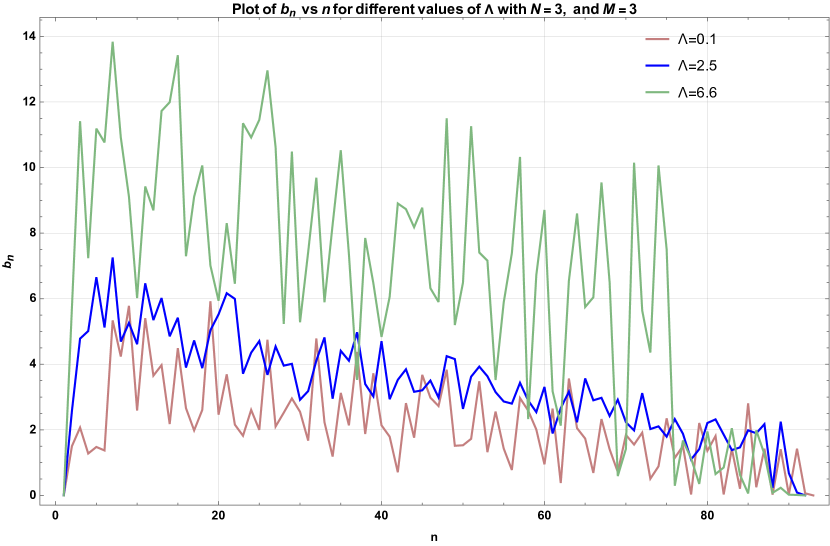
(a) Lanczos sequence for M=3, N=3.

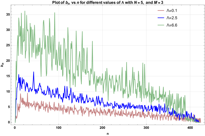
(b) Lanczos sequence for M=3, N=5.

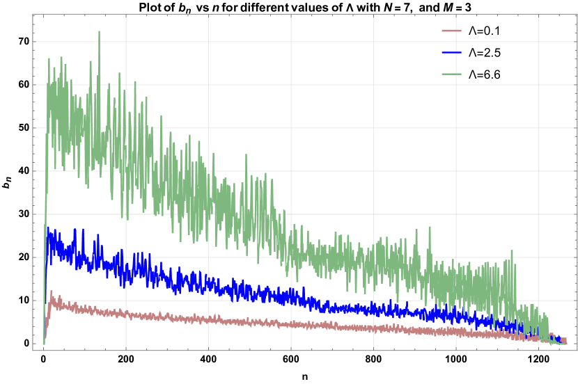
(c) Lanczos sequence for M=3, N=7

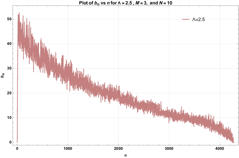
(d) Lanczos sequence for M=3, N=10

Figure 1: Lanczos sequence for different configurations of M, and N. Fig.(1(a)) shows the Lanczos sequence for N=3, and M=3, Fig.(1(b)) for N=5, and M=3, and Fig.(1(c)) for N=7, and M=3 respectively for the values of $\Lambda=0.1,2.5,6.6$. Fig.(1(d)) plots the Lanczos coefficients $b_{n}$ for $\Lambda=2.5$, N=10, and M=3. For all the cases, the Lanczos coefficients $b_{n}$ initially grows linearly with n up to $n\sim\ln{D}$, and then slowly decrease to zero with a slope of order $\sim-\frac{1}{D^{2}}\sim-\frac{1}{K}$. The Lanczos sequence $\{b_{n}\}$ smoothens as we increase the system size.

We restrict our analysis to the a three-site Bose-Hubbard model with particle numbers $N=3,5,7$. We state our numerical results for the three-site Bose-Hubbard model with an initial operator mentioned in Eq.(18), and for different values of interaction strength parameter $\Lambda$ as following:

• For $\Lambda=0$, the Lanczos iteration stops at the fifth iterative order with $b_{5}=0$. So, the dimension $K=4$ of Krylov basis is much smaller than the dimension of the Hilbert space of operators $D^{2}=100$ and hence, confirms the bound mentioned in Eq.(8). For smaller values of $\Lambda\sim 10^{-7}-10^{-3}$, the Lanczos iteration stops at the fifth iterative order with $b_{5}\sim 10^{-6}.$ This kind of behavior is expected as the Bose-Hubbard model is learned to be integrable Nakerst:2022prc for $\Lambda\rightarrow 0$ as $\Lambda=0$ or $U=0$ is just a Gaussian model and hence this is consistent.

• Similarly, for large $\Lambda\sim 10^{15}$, the Lanczos iteration stops at a very small value of $K$, which is in agreement with the integrable nature of the Bose-Hubbard model at $\Lambda\rightarrow\infty$ Nakerst:2022prc as in this limit, the only possible Lyaponuv exponent is found to be exactly zero.

• The Lanczos iteration saturates the upper bound mentioned in Eq.(8) for finite values of $\Lambda$. The plots of $b_{n}$ with $n$ show a phase of initial growth up to $n\sim\ln{D}$. The initial phase of growth is then followed by a regime of steady decrease towards zero with a generally constant negative slope of the order $\sim-10^{-2}\sim K^{-1}$. This is shown in the Fig. (1(a)), (1(b)) and (1(c)) for different values of $(M,N)$.

These observations suggest that the operator growth via the nature of the Lanczos coefficients can distinguish the system as being chaotic or non-chaotic (integrable), providing further evidence to the earlier claims Parker:2018yvk ; Rabinovici:2022beu ; Rabinovici:2021qqt . We summarize our conclusions regarding the nature of the Lanczos coefficients in the Table 1.

$\mathbf{n}$	Nature of Lanczos coefficients $\mathbf{b_{n}}$
$1<<n<\ln{D}$	$b_{n}$ grows linearly with n: $b_{n}\sim c\,n$
$\ln{D}<<n<D^{2}$	a steady fall-off of $b_{n}$ with n having slope $\sim\frac{1}{K}$
$n\sim D^{2}$	$b_{n}$ falls off to zero

Table 1: The table summarises different behaviors of Lanczos coefficients $b_{n}$ with n for a chaotic system having the dimension of Krylov basis $K$.

Variance of Lanczos coefficients

Before we end the section, we numerically study the variance of ${b_{n}}$ due to their fluctuating behaviour, for the integrable and chaotic regimes as a function of the parameter $\Lambda$.

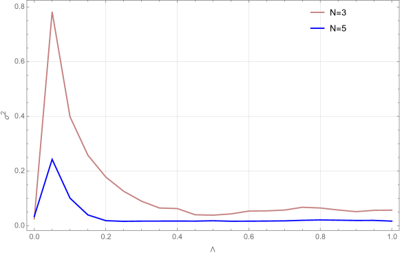
Figure 2: The above figure plots the variance $\sigma^{2}$ as a function of the interaction parameter $\Lambda$ for $(N,M)=(3,3),(3,5)$. It can be seen from the plot that as $\Lambda$ becomes finite starting from $\Lambda=0$, the variance decreases and becomes close to zero for $\Lambda=1$. This behaviour of the variance points towards the transition from integrable to chaotic.

• In Fig. 2, we have shown the nature of the variance $\sigma^{2}$ as a function of the interaction parameter $\Lambda$. We notice that as the value of the parameter $\Lambda$ increases from 0 to 1, the variance $\sigma^{2}$ becomes closer to zero. The above behavior of the variance is typically true for chaotic systems Hashimoto:2023swv ; Rabinovici:2021qqt and hence we conclude that the system is integrable for $\Lambda=0$ and becomes more and more chaotic as $\Lambda$ approaches the value 1.

• Also, as we increase the system size, the Lanczos sequence smoothens out for the chaotic system, bringing the variance closer to zero and causing a more smooth transition from the integrable regime, $\Lambda=0$ to the chaotic one $\Lambda>0$.

• One can notice a sharp fall-off in $\sigma^{2}$ values as the value of the $\Lambda$ increases from zero. It marks the transistion of the system from a integrable to a chaotic one as was expected from our previous analysis of the Lanczos coefficients.

• Also, one can find that a similar sharp peak can be obtained at $\Lambda\sim\mathcal{O}(10^{2})$ which marks the transition from chaotic to an integrable system.

• Also, in Fig. 2 one can notice “kinks” near $\Lambda\sim 0.1$, $\Lambda\sim 0.15$ etc. These kinks are due to the unsmooth behavior of Lanczos coefficients for small system size. As we increase the system size and $b_{n}$s become smooth, these kinks disappear. One can immediately get a hint of this from the $N=5$ plot where some of the kinks disappear.

We have listed our findings from the numerical analysis of $b_{n}$ pointwise above where we have analysed three-site Bose-Hubbard model for different system configurations. Note that the disordered average of $b_{n}$ has been considered in Rabinovici:2020ryf for the SYK₄ model and in Trigueros:2021rwj for a many-body localization (MBL) systems, e.g., one-dimensional (1D) spin chain with $L$ sites and open boundary conditions, where in both cases values for the interaction strengths are drawn randomly from a certain random distribution and then $\{b_{n}\}$ are averaged over all the random realizations. The interaction parameter $\Lambda$ in the Bose-Hubbard model does not follow from a random distribution. We do our analysis for particular values of $\Lambda$ to characterize the chaotic and non-chaotic (integrable) behaviour.

7 Krylov Complexity

Now we investigate the Krylov complexity, often termed as K-complexity that was introduced by Parker et.al Parker:2018yvk as a useful diagnostic of quantum chaos in thermodynamic limit which measures an operator’s complexification over the orthonormal Krylov basis. Parker:2018yvk . Also motivated by our study of the variance of Lanczos coefficients in the previous section, we will mainly focus on the finite $\Lambda$ regime where the model is expected to show chaotic behaviour. It is obtained by first constructing the Krylov basis using the Lanczos algorithm given by (5) and then using the Lanczos coefficients $b_{n}$ to reduce the analysis of the time-evolution of an operator $\mathcal{O}$ into the solution of a differential recurrence equation Parker:2018yvk . The definition of Krylov complexity is outlined below.

The time-evolved operator can be expanded in the Krylov basis as:

$$|\mathcal{O}(t))=e^{it\mathcal{L}}|\mathcal{O})=\sum_{n=0}^{K-1}\phi_{n}(t)|\mathcal{O}_{n}),$$ (13)

where $\phi_{n}(t)$ can be thought of as single-particle wavefunctions distributed over the Krylov basis, which via the Heisenberg equation $\frac{d\mathcal{O}}{dt}=i[H,\mathcal{O}]$ satisfies the following differential recurrence equation,

$$-i\dot{\phi}_{n}(t)=\sum_{m=0}^{K-1}L_{mn}\phi_{m}(t)=b_{n+1}\phi_{n+1}(t)+b_{n}\phi_{n-1}(t).$$ (14)

To solve this equation we need an initial conditions which is:

$$\phi_{n}(t=0)=\delta_{n0},$$

For a normalised operator $\mathcal{O}(0)=\mathcal{O}_{0}$, and $\phi_{-1}(t)\equiv 0$ to make Eq. (14) consistent with Eq. (13) we need to impose this initial condition. Furthermore, the boundary conditions $b_{0}=b_{K}=0$ are fixed to ensure the finiteness of this operator-evolution problem. One can also infer from the equation of motion mentioned Eq. (14) of the wavefunctions $\phi_{n}(t)$ as a single-particle hopping problem on a semi-infinite chain called the Krylov chain, with the hopping amplitudes given by the Lanczos coefficients $b_{n}$ and $\phi_{n}(t)$ are the wave-packets traveling on the chain Parker:2018yvk . Since the initial operator is normalized at the first step of the Lanczos algorithm mentioned in Sec. (5), the notion of unitarity suggests that the wavefunction $\phi_{n}(t)$ is normalized at all times:

$$\sum_{n=0}^{K-1}|\phi_{n}(t)|^{2}=1.$$

Then Krylov complexity or K-complexity is defined as the time-dependent average position of the distribution $\phi_{n}(t)$ over the ordered Krylov basis Parker:2018yvk :

$$\mathcal{C}_{K}(t)=\sum_{n=0}^{K-1}n|\phi_{n}(t)|^{2}.$$ (15)

We discuss the behavior of the K-complexity emerging from the numerical analysis in the following points:

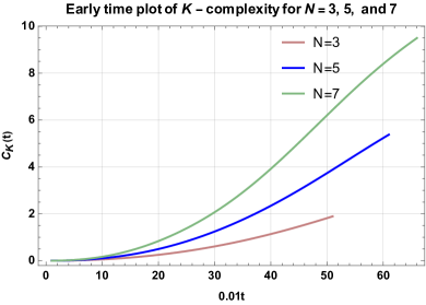
Figure 3: Early time plot (scrambling) of Krylov complexity $C_{K}(t)$ for $\Lambda=2.5$ with time t. The magenta, blue, and green line represents plot of $C_{K}(t)$ for $\{N=3,M=3,t_{s}=0.36\}$, $\{N=5,M=3,t_{s}=0.48\}$, $\{N=7,M=3,t_{s}=0.55\}$ respectively.

• We observe an exponential growth in K-complexity $\mathcal{C}_{K}(t)$ at very early times until $t_{s}=\log{(\log{D})}$. This is known as the scrambling time. The value of scrambling time $t_{s}$ changes as the system configuration changes which is shown in Fig. 3.

  

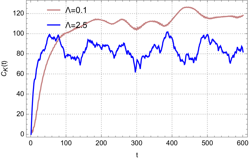
  (a)

  

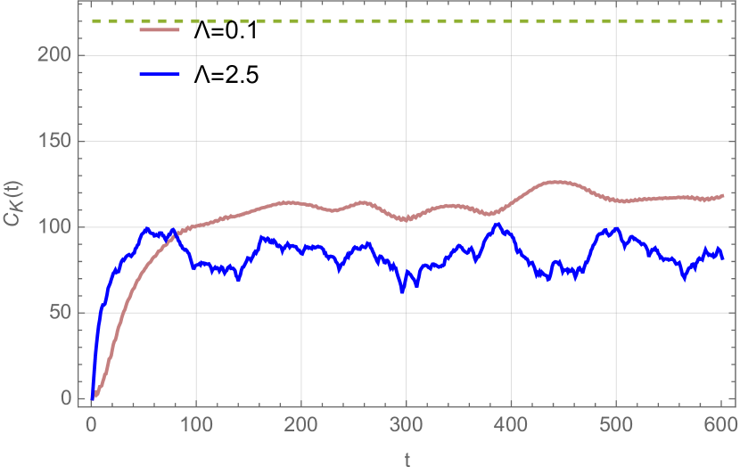
  (b)

  Figure 4: Plot of K-complexity at all time scales for $\Lambda=0.1,2.5$ with $N=5$, and $M=3$. The linear growth and the saturation can be observed at times of $\mathcal{O}(D)$, and at $\mathcal{O}(D^{2})$ respectively. For $N=5$, and $M=3$, $D=441$ and $K=421$. The saturation value of $\mathcal{C}_{k}(t)$ is $\frac{K}{2}=220$ is shown by the dashed line in the second figure.

• After the scrambling time $t_{s}$, the K-complexity $\mathcal{C}_{K}(t)$ features a linear increase in time until times of order $t\sim D$ and finally at very late times of order $t\sim D^{2}$ it saturates (with fluctuations around that saturation value as shown in Fig. 4) typically at the values of order $\frac{K}{2}$. This phenomenon can be understood physically as a uniform distribution of operator in Krylov basis. The behavior of the K-complexity at all time scales is shown in Fig. 4 for different values interaction parameter $\Lambda$.

The above results are summarised in Table 2. The characteristics of K-complexity described above clearly agree with the results of Barbon:2019wsy where the profile of K-complexity for generic operators in a finite-size system was first shown . One can refer to Appendix.(B) where numerical fit is performed to analyse the behaviour of K-complexity at different time scales.

$\mathbf{t}$	Nature of Krylov complexity $\mathbf{C_{K}(t)}$
$0\leq t\leq\log{(\ln{D})}$	$C_{K}(t)$ grows exponentially in time t : $C_{K}(t)\sim\exp{c\,t}$
$t\sim D$	linear growth of $\mathcal{C}_{K}(t)$ with t
$t\sim D^{2}$	$C_{K}(t)$ saturates

Table 2: The table distinguishes different behaviors of Krylov complexity $C_{K}(t)$ with t for a chaotic system.

8 Discussion

In this article, we considered the Bose-Hubbard model as a quantum many-body model that is neither integrable nor strongly chaotic. It also has a quartic term in the Hamiltonian, providing a platform to study Krylov complexity beyond the quadratic discrete bosonic quantum many-body system. The ultra-cold atom Hamiltonian is directly related to the Bose-Hubbard Hamiltonian. We investigate a considerably more basic form of the model with a chemical potential $\mu=0$ and, thus, does not exhibit any phase transition.

We start by analyzing the operator growth in Krylov basis in a three-site $(M=3)$ Bose-Hubbard model for different parameter $\Lambda$ values. Furthermore, we perform a numerical analysis to explore operator growth in the Bose-Hubbard model. We study cases with different particle sizes, $N$. Although we have shown the results for a specific initial operator, overall features remain the same even if we consider different initial operators. An important observation of our work is that the standard method of performing the Lanczos algorithm fails for this model due to the piling of errors at each level of the iteration. We remove this difficulty by performing the Full orthogonalization (FO) method to find the appropriate Krylov basis and the Lanczos coefficients.

One of our crucial findings was that the dimension of the Krylov basis $(K)$ is much smaller than the dimension of the Hilbert space for the operators when $\Lambda\rightarrow 0$ or $\Lambda\rightarrow\infty$. This confirms the fact that the three-site Bose-Hubbard model becomes integrable at the asymptotic limits of $\Lambda$. The Lanczos coefficient $b_{n}$ displays ramp and plateau behaviour for finite values of $\Lambda$. This indicates that for finite values of $\Lambda$, the three-site Bose-Hubbard model becomes chaotic, and the dimension of the Krylov basis saturates the upper bound as mentioned in Eq. (8). Also, in addition to the study of the behaviour of Lanczos coefficients $b_{n}$, we also study the variance $\sigma^{2}$ of the Lanczos sequence as a function of the interaction parameter $\Lambda$ which arises naturally as $\{b_{n}\}$ are fluctuating in nature. We observed that the variance follows the typical nature of being close to zero Hashimoto:2023swv as we approach from an integrable system to a chaotic one. It will be interesting to figure out in future how we can extract the information about spectral statistics, which encodes the information of the quantum chaos from the statistics of $b_{n}$ perhaps following the study of Erdmenger:2023shk ; Hashimoto:2023swv .

Furthermore, we investigate the Krylov complexity for finite $\Lambda$. We have investigated the behaviour of K-complexity at three different time scales. We discovered that the K-complexity exhibits exponential increase at initial time scales, typically of $\mathcal{O}(\log(\ln{D}))$, followed by a linear growth over time. K-complexity saturates in time at very late times, of the order of the dimension of the operator Hilbert space. This demonstrates that the three-site Bose-Hubbard model becomes chaotic for finite $\Lambda$. The emergence of these three distinct time scales matches with the general claim made in the literature, e.g. Barbon:2019wsy .

There are various future directions that will be interesting to pursue. One can study the Liouvillian spectrum and operator matrix elements in energy eigenbasis to find universal chaotic behaviour of the system from ETH approachprogress . Throughout our studies, we have set the chemical potential to zero. However, the system can undergo quantum phase transitions in the presence of non-vanishing chemical potential. It will be interesting to perform our analysis for this case and whether we can comment on the phase transition using Krylov complexity. This will provide a possibility of comparing with the results coming from the circuit complexity analysis for the Bose-Hubbard model as well as connecting with results from holography Sood:2021cuz ; Sood:2022lfx ; Huang:2021xjl . Also, it will be interesting to extend our computation for finite temperature case and compare with the results of Avdoshkin:2019trj ; Avdoshkin:2022xuw ; Camargo:2022rnt whether we get a staggered-like behaviour for Lanczos coefficients. Recently emergence is scar-like states which evade thermalization has been demonstrated in Bose-Hubbard type models 2020PhRvL.124p0604Z ; 2022arXiv221212046H ; Su:2022glk . It will be interesting to study the (spread) complexity of such states along the line of Nandy:2023brt . Furthermore, we like the continuous limit of this model study the Krylov complexity and hope to connect with the recent studies of it for field theories Avdoshkin:2019trj ; Camargo:2022rnt ; Dymarsky:2021bjq . We hope to address some of these issues in the near future and report on them. Last but not least, as mentioned earlier, the Bose-Hubbard model emerges from various physical scenarios involving ultra-cold atom gas in periodic potential (e.g. dimerized magnets 2012arXiv1210.1270L , interaction-induced tunnelling 2012PhRvL.108k5301S ) and can potentially be used as a quantum-simulator Yang:2020yer , we hope that our study of operator growth and the associated complexity for this system might shed important light in this context and initiate further studies.

Appendix A An alternate choice of initial operator

In this section, we provide the numerical results obtained from studying the Lanczos coefficients and Krylov complexity for a choice of the initial operator that is different from the initial operator considered in the main text. We work in $M=3$ and $N=5$ system. The appropriate hermitian operator that we choose for numerical computations is given by the number operator at the first and second sites:

$$\mathcal{O}_{\text{in}}=\hat{n}_{1}+\hat{n}_{2}$$ (16)

The numerical results obtained are shown in the Fig (5). One can take other choices of different hermitian operators that do not commute with the Bose-Hubbard Hamiltonian (1). For instance, the choice of the initial operator where the number operator at all sites is taken commute with the Hamiltonian (1) and thus makes the Lanczos algorithm trivial.

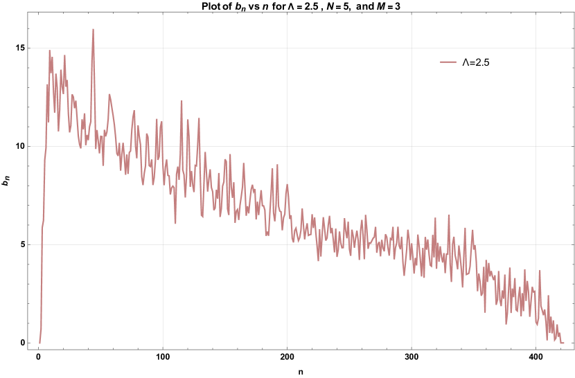
(a)

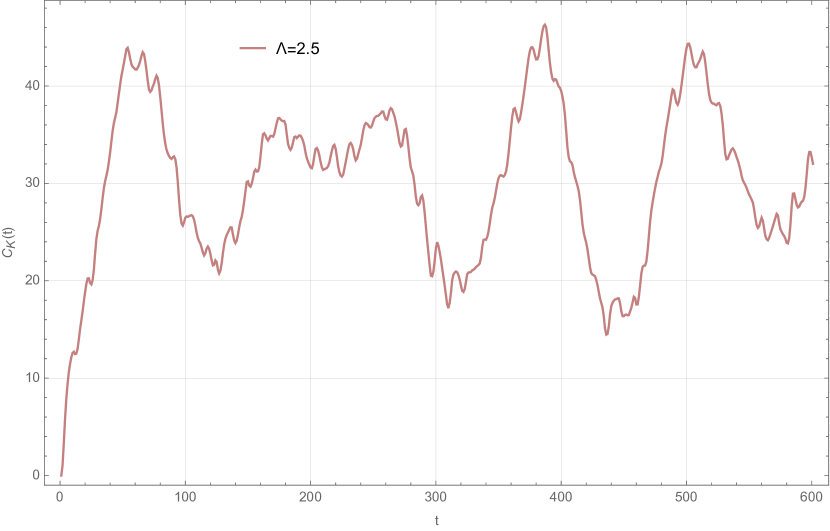
(b)

Figure 5: Lanczos sequence Fig.(5(a)) and K-complexity Fig.(5(b)) for a different choice of initial operator (16). Fig.(5(a)) shows the Lanczos sequence for $N=5$, and $M=3$. One can easily see and relate to the previous results and conclude that the Lanczos coefficients $b_{n}$ initially grow linearly with n up to $n\sim\ln{D}$, and then slowly decrease to zero with a slope of order $\sim-\frac{1}{D^{2}}\sim-\frac{1}{K}$. Fig.(5(b)) plots K-complexity at all time scales for $\Lambda=2.5$ with $N=5$, and $M=3$. The linear growth and the saturation can be observed at times of $\mathcal{O}(D)$, and at $\mathcal{O}(D^{2})$ respectively. For $N=5$, and $M=3$, $D=441$ and $K\sim 421$.

Appendix B Numerical fits of K-complexity at different time scales

Below we discuss the numerical fits done to obtain the different behaviours of $C_{k}(t)$ at different time scales. We have shown a case where $\Lambda=0.1$, $N=5$, and $M=3$. We found that the exponent $\alpha=0.49635$ controlling the exponential behaviour of K-complexity at early times is approximately equal to the slope of $b_{n}$, $\beta=0.53538$ in the linear regime as was expected.

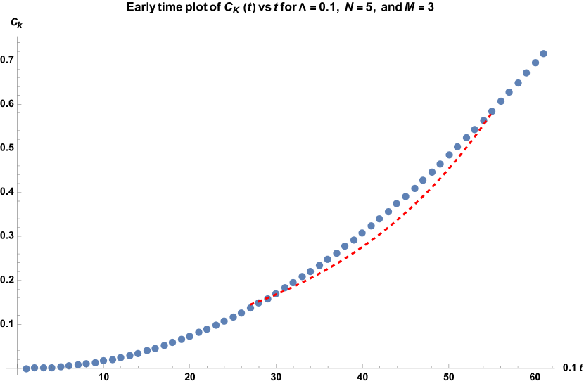
(a)

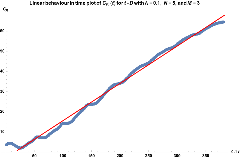
(b)

Figure 6: Plot of K-complexity at all different scales for $\Lambda=0.1$ with $N=5$, and $M=3$. Numerical fits are included at both the early time plot in Fig.(6(a)) near the scrambling time $t_{s}=0.48$ and at times $\sim\mathcal{O}(D)$ in Fig.(6(b)) respectively. Fig.(6(a)) shows the exponential growth of K-complexity at early times ($t\sim\log(lnD)$). The non-linear fit function is $C_{K}(t)=0.0379053\,\exp{(0.49635\,t)}$ with $r^{2}=0.989944$ denoted by red dashed lines. Fig.(6(b)) shows the linear growth of K-complexity at times of $\mathcal{O}(D)$.The linear fit function is given by $C_{K}(t)=-2.92944+1.85039\,t$ with $r^{2}=0.992016$ denoted by red line.

Appendix C More on the operator growth and Lanczos coefficients

We give an example of the growth of the operator in the Krylov basis. Given the Hamiltonian in 1, and the general form of the initial operator in 12, we examine the steps of the Lanczos algorithm. We use the notion of Frobenius inner product defined in 9 and the bosonic commutation relation is given by

$$[a_{n},a^{{\dagger}}_{n}]=1\,,$$ (17)

where the subscript $n$ represents the site number. We start with the three-particle and three-site Bose-Hubbard model where $\Lambda=2.5$, and the initial operator is given by

$$\mathcal{O}_{ini}=\hat{n}_{1}+\hat{n}_{2}-i(a^{{\dagger}}_{1}a_{2}-a^{{\dagger}}_{2}a_{1})$$ (18)

where $\hat{n}_{1}=a^{{\dagger}}_{1}a_{1}$ and $\hat{n}_{2}=a^{{\dagger}}_{2}a_{2}$ are the number operators on the 1st and 2nd site respectively.

• $\mathcal{O}_{0}$: The operator $\mathcal{O}_{ini}$ is not normalised. We normalise it using the inner product defined in 9 to get our starting operator $\mathcal{O}_{0}$ as:

  $$|\mathcal{O}_{0})=\frac{1}{||\mathcal{O}_{ini}||}|\mathcal{O}_{ini})=0.353|\mathcal{O}_{ini}).$$ (19)

• $\mathcal{O}_{1}$: Computing $\mathcal{O}_{1}$ needs the evaluation of $\mathcal{A}_{1}$:

  $$\mathcal{A}_{1}=[H,\mathcal{O}_{0}]\,.$$ (20)

  Next, we perform reorthogonalization on $\mathcal{A}_{1}$ by writing

  $$|\mathcal{A}_{1})\longrightarrow|\mathcal{A}_{1})-|\mathcal{O}_{0})(\mathcal{O}_{0}|\mathcal{A}_{1})$$ (21)

  and get

  $$\mathcal{A}_{1} = 0.707i(\hat{n}_{2}-\hat{n}_{1})+0.353(a^{{\dagger}}_{2}a_{3}-a^{{\dagger}}_{3}a_{2}-i\,a^{{\dagger}}_{1}a_{3}-i\,a^{{\dagger}}_{3}a_{1})+$$ (22)

  $$0.884\,i\,(a^{{\dagger}}_{2}a^{{\dagger}}_{1}a_{2}a_{2}+a^{{\dagger}}_{2}a^{{\dagger}}_{2}a_{2}a_{1}-a^{{\dagger}}_{1}a^{{\dagger}}_{1}a_{2}a_{1}-a^{{\dagger}}_{2}a^{{\dagger}}_{1}a_{1}a_{1})\,.$$

  The first Lanczos coefficient is:

  $$b_{1}=\sqrt{(\mathcal{A}_{1}|\mathcal{A}_{1})}=2.574.$$ (23)

  The matrix representation of the operators $\mathcal{A}$ is written in the $D=10$ dimensional Hilbert space. As a result, at this level of iteration, the orthogonalized Krylov operator is:

  $$\mathcal{O}_{1}=\frac{1}{b_{1}}\,|\mathcal{A}_{1}) = 0.275\,i(\hat{n}_{2}-\hat{n}_{1})+0.137(a^{{\dagger}}_{2}a_{3}-a^{{\dagger}}_{3}a_{2}-i\,a^{{\dagger}}_{1}a_{3}-ia^{{\dagger}}_{3}a_{1})+$$ (24)

  $$0.343\,i\,(a^{{\dagger}}_{2}a^{{\dagger}}_{1}a_{2}a_{2}+a^{{\dagger}}_{2}a^{{\dagger}}_{2}a_{2}a_{1}-a^{{\dagger}}_{1}a^{{\dagger}}_{1}a_{2}a_{1}-a^{{\dagger}}_{2}a^{{\dagger}}_{1}a_{1}a_{1})\,.$$

  Note that, the operator $\mathcal{O}_{0}$ is a double-site operator. It grows to $\mathcal{O}_{1}$, which is a mix of double-site and quadruple-site operators. At the next step, the operator $\mathcal{O}_{1}$ will grow to a six-site operator contribution to give $\mathcal{O}_{2}$. However, the operators cannot grow more than a six-site contribution because of the restriction on the total number of particles $N=3$. Thus, the operator remains as a six-site operator until it exhausts all the linearly independent contributions. The rest of the orthonormal operators of the Krylov basis can be generated using the same approach. In this case, the algorithm terminates at the $n=92$ level of iteration giving $b_{92}=0$. Hence the Krylov dimension is $K=91$ which exactly saturates the bound mentioned in 8. For a larger value of $N$, the operator growth does not stop at a six-site operator. Hence, the analysis becomes more and more tedious and can be performed by a numerical analysis owing to the results in the main text.

References

- (1) C. von Keyserlingk, T. Rakovszky, F. Pollmann and S. Sondhi, Operator hydrodynamics, OTOCs, and entanglement growth in systems without conservation laws, Phys. Rev. X 8 (2018) 021013 [1705.08910].
- (2) A. Nahum, S. Vijay and J. Haah, Operator Spreading in Random Unitary Circuits, Phys. Rev. X 8 (2018) 021014 [1705.08975].
- (3) V. Khemani, A. Vishwanath and D. A. Huse, Operator spreading and the emergence of dissipation in unitary dynamics with conservation laws, Phys. Rev. X 8 (2018) 031057 [1710.09835].
- (4) T. Rakovszky, F. Pollmann and C. W. von Keyserlingk, Diffusive hydrodynamics of out-of-time-ordered correlators with charge conservation, Phys. Rev. X 8 (2018) 031058 [1710.09827].
- (5) S. Gopalakrishnan, D. A. Huse, V. Khemani and R. Vasseur, Hydrodynamics of operator spreading and quasiparticle diffusion in interacting integrable systems, Phys. Rev. B 98 (2018) 220303 [1809.02126].
- (6) A. I. Larkin and Y. N. Ovchinnikov, Quasiclassical Method in the Theory of Superconductivity, Soviet Journal of Experimental and Theoretical Physics 28 (1969) 1200.
- (7) S. Xu and B. Swingle, Locality, Quantum Fluctuations, and Scrambling, Phys. Rev. X 9 (2019) 031048 [1805.05376].
- (8) Y. Gu, A. Kitaev and P. Zhang, A two-way approach to out-of-time-order correlators, JHEP 03 (2022) 133 [2111.12007].
- (9) J. Maldacena, S. H. Shenker and D. Stanford, A bound on chaos, JHEP 08 (2016) 106 [1503.01409].
- (10) J. Maldacena and D. Stanford, Remarks on the Sachdev-Ye-Kitaev model, Phys. Rev. D 94 (2016) 106002 [1604.07818].
- (11) A. Kitaev, A simple model of quantum holography, .
- (12) S. Sachdev and J. Ye, Gapless spin-fluid ground state in a random quantum heisenberg magnet, Phys. Rev. Lett. 70 (1993) 3339.
- (13) B. V. Fine, T. A. Elsayed, C. M. Kropf and A. S. de Wijn, Absence of exponential sensitivity to small perturbations in nonintegrable systems of spins 1/2, Phys. Rev. E 89 (2014) 012923.
- (14) S. Xu and B. Swingle, Accessing scrambling using matrix product operators, Nature Phys. 16 (2019) 199 [1802.00801].
- (15) D. E. Parker, X. Cao, A. Avdoshkin, T. Scaffidi and E. Altman, A Universal Operator Growth Hypothesis, Phys. Rev. X 9 (2019) 041017 [1812.08657].
- (16) J. L. F. Barbón, E. Rabinovici, R. Shir and R. Sinha, On The Evolution Of Operator Complexity Beyond Scrambling, JHEP 10 (2019) 264 [1907.05393].
- (17) E. Rabinovici, A. Sánchez-Garrido, R. Shir and J. Sonner, Operator complexity: a journey to the edge of Krylov space, JHEP 06 (2021) 062 [2009.01862].
- (18) S.-K. Jian, B. Swingle and Z.-Y. Xian, Complexity growth of operators in the SYK model and in JT gravity, JHEP 03 (2021) 014 [2008.12274].
- (19) A. Dymarsky and A. Gorsky, Quantum chaos as delocalization in krylov space, Phys. Rev. B 102 (2020) 085137.
- (20) D. J. Yates, A. G. Abanov and A. Mitra, Lifetime of almost strong edge-mode operators in one-dimensional, interacting, symmetry protected topological phases, Phys. Rev. Lett. 124 (2020) 206803.
- (21) D. J. Yates, A. G. Abanov and A. Mitra, Dynamics of almost strong edge modes in spin chains away from integrability, Physical Review B 102 (2020) .
- (22) E. Rabinovici, A. Sánchez-Garrido, R. Shir and J. Sonner, Krylov localization and suppression of complexity, JHEP 03 (2022) 211 [2112.12128].
- (23) D. J. Yates, A. G. Abanov and A. Mitra, Long-lived period-doubled edge modes of interacting and disorder-free Floquet spin chains, 2105.13766.
- (24) D. J. Yates and A. Mitra, Strong and almost strong modes of Floquet spin chains in Krylov subspaces, Phys. Rev. B 104 (2021) 195121 [2105.13246].
- (25) A. Dymarsky and M. Smolkin, Krylov complexity in conformal field theory, Phys. Rev. D 104 (2021) L081702 [2104.09514].
- (26) J. D. Noh, Operator growth in the transverse-field ising spin chain with integrability-breaking longitudinal field, Physical Review E 104 (2021) .
- (27) F. B. Trigueros and C.-J. Lin, Krylov complexity of many-body localization: Operator localization in Krylov basis, 2112.04722.
- (28) C. Liu, H. Tang and H. Zhai, Krylov complexity in open quantum systems, 2022. 10.48550/ARXIV.2207.13603.
- (29) Z.-Y. Fan, Universal relation for operator complexity, Physical Review A 105 (2022) .
- (30) A. Kar, L. Lamprou, M. Rozali and J. Sully, Random matrix theory for complexity growth and black hole interiors, Journal of High Energy Physics 2022 (2022) .
- (31) P. Caputa, J. M. Magan and D. Patramanis, Geometry of krylov complexity, 2021. 10.48550/ARXIV.2109.03824.
- (32) R. Heveling, J. Wang and J. Gemmer, Numerically probing the universal operator growth hypothesis, Phys. Rev. E 106 (2022) 014152.
- (33) K. Adhikari, S. Choudhury and A. Roy, rylov omplexity in uantum ield heory, 2022. 10.48550/ARXIV.2204.02250.
- (34) B. Bhattacharjee, S. Sur and P. Nandy, Probing quantum scars and weak ergodicity breaking through quantum complexity, Phys. Rev. B 106 (2022) 205150 [2208.05503].
- (35) B. Bhattacharjee, X. Cao, P. Nandy and T. Pathak, Krylov complexity in saddle-dominated scrambling, Journal of High Energy Physics 2022 (2022) .
- (36) B.-n. Du and M.-x. Huang, Krylov Complexity in Calabi-Yau Quantum Mechanics, 2212.02926.
- (37) A. Banerjee, A. Bhattacharyya, P. Drashni and S. Pawar, From CFTs to theories with Bondi-Metzner-Sachs symmetries: Complexity and out-of-time-ordered correlators, Phys. Rev. D 106 (2022) 126022 [2205.15338].
- (38) W. Mück and Y. Yang, Krylov complexity and orthogonal polynomials, 2022. 10.48550/ARXIV.2205.12815.
- (39) A. Bhattacharya, P. Nandy, P. P. Nath and H. Sahu, Operator growth and krylov construction in dissipative open quantum systems, 2022. 10.48550/ARXIV.2207.05347.
- (40) N. Hörnedal, N. Carabba, A. S. Matsoukas-Roubeas and A. del Campo, Ultimate speed limits to the growth of operator complexity, Communications Physics 5 (2022) .
- (41) S. Guo, Operator growth in su(2) yang-mills theory, 2022. 10.48550/ARXIV.2208.13362.
- (42) B. Bhattacharjee, X. Cao, P. Nandy and T. Pathak, An operator growth hypothesis for open quantum systems, 2212.06180.
- (43) E. Rabinovici, A. Sánchez-Garrido, R. Shir and J. Sonner, Krylov complexity from integrability to chaos, JHEP 07 (2022) 151 [2207.07701].
- (44) M. Alishahiha and S. Banerjee, A universal approach to Krylov State and Operator complexities, 2212.10583.
- (45) A. Avdoshkin, A. Dymarsky and M. Smolkin, Krylov complexity in quantum field theory, and beyond, 2212.14429.
- (46) A. Kundu, V. Malvimat and R. Sinha, State Dependence of Krylov Complexity in CFTs, 2303.03426.
- (47) E. Rabinovici, A. Sánchez-Garrido, R. Shir and J. Sonner, A bulk manifestation of Krylov complexity, 2305.04355.
- (48) R. Zhang and H. Zhai, Universal Hypothesis of Autocorrelation Function from Krylov Complexity, 2305.02356.
- (49) A. A. Nizami and A. W. Shrestha, Krylov construction and complexity for driven quantum systems, 2305.00256.
- (50) K. Hashimoto, K. Murata, N. Tanahashi and R. Watanabe, Krylov complexity and chaos in quantum mechanics, 2305.16669.
- (51) S. Nandy, B. Mukherjee, A. Bhattacharyya and A. Banerjee, Quantum state complexity meets many-body scars, 2305.13322.
- (52) V. Balasubramanian, P. Caputa, J. M. Magan and Q. Wu, Quantum chaos and the complexity of spread of states, Phys. Rev. D 106 (2022) 046007 [2202.06957].
- (53) V. Balasubramanian, M. DeCross, A. Kar, Y. C. Li and O. Parrikar, Complexity growth in integrable and chaotic models, JHEP 07 (2021) 011 [2101.02209].
- (54) P. Caputa and S. Liu, Quantum complexity and topological phases of matter, Phys. Rev. B 106 (2022) 195125.
- (55) P. Caputa, N. Gupta, S. S. Haque, S. Liu, J. Murugan and H. J. R. Van Zyl, Spread complexity and topological transitions in the Kitaev chain, JHEP 01 (2023) 120 [2208.06311].
- (56) M. Afrasiar, J. K. Basak, B. Dey, K. Pal and K. Pal, Time evolution of spread complexity in quenched lipkin-meshkov-glick model, 2022. 10.48550/ARXIV.2208.10520.
- (57) J. Erdmenger, S.-K. Jian and Z.-Y. Xian, Universal chaotic dynamics from Krylov space, 2303.12151.
- (58) A. Bhattacharya, P. Nandy, P. P. Nath and H. Sahu, On Krylov complexity in open systems: an approach via bi-Lanczos algorithm, 2303.04175.
- (59) A. Chattopadhyay, A. Mitra and H. J. R. van Zyl, Spread complexity as classical dilaton solutions, 2302.10489.
- (60) K. Pal, K. Pal, A. Gill and T. Sarkar, Time evolution of spread complexity and statistics of work done in quantum quenches, 2304.09636.
- (61) D. Jaksch, C. Bruder, J. I. Cirac, C. W. Gardiner and P. Zoller, Cold bosonic atoms in optical lattices, Physical Review Letters 81 (1998) 3108.
- (62) S. Sachdev, Quantum Phase Transitions. Cambridge University Press, 1999.
- (63) K. Sengupta and N. Dupuis, Mott-insulator–to–superfluid transition in the bose-hubbard model: A strong-coupling approach, Physical Review A 71 (2005) .
- (64) S. Mossmann and C. Jung, Semiclassical approach to bose-einstein condensates in a triple well potential, Phys. Rev. A 74 (2006) 033601.
- (65) T. F. Viscondi and K. Furuya, Dynamics of a bose einstein condensate in a symmetric triple-well trap, Journal of Physics A: Mathematical and Theoretical 44 (2011) 175301.
- (66) M. Rautenberg and M. Gärttner, Classical and quantum chaos in a three-mode bosonic system, Phys. Rev. A 101 (2020) 053604.
- (67) M. Feingold and A. Peres, Regular and chaotic motion of coupled rotators, Physica D: Nonlinear Phenomena 9 (1983) 433.
- (68) M. Feingold, N. Moiseyev and A. Peres, Ergodicity and mixing in quantum theory. ii, Phys. Rev. A 30 (1984) 509.
- (69) D. Wintgen and H. Friedrich, Classical and quantum-mechanical transition between regularity and irregularity in a hamiltonian system, Phys. Rev. A 35 (1987) 1464.
- (70) G. Nakerst and M. Haque, Chaos in the three-site Bose-Hubbard model: Classical versus quantum, Phys. Rev. E 107 (2023) 024210 [2203.09953].
- (71) V. Balasubramanian, J. M. Magan and Q. Wu, A Tale of Two Hungarians: Tridiagonalizing Random Matrices, 2208.08452.
- (72) H. A. Camargo, V. Jahnke, K.-Y. Kim and M. Nishida, Krylov complexity in free and interacting scalar field theories with bounded power spectrum, JHEP 05 (2023) 226 [2212.14702].
- (73) M. Pinkwart, Thermalization and Integrability in the one-dimensional Bose-Hubbard Model, 2014.
- (74) J. M. Zhang and R. X. Dong, Exact diagonalization: the bose–hubbard model as an example, European Journal of Physics 31 (2010) 591.
- (75) C. Lanczos, An iteration method for the solution of the eigenvalue problem of linear differential and integral operators, J. Res. Natl. Bur. Stand. B 45 (1950) 255.
- (76) V. Viswanath and G. Müller, The recursion method: Application to many body dynamics, .
- (77) B. Parlett, The Symmetric Eigenvalue Problem, Classics in Applied Mathematics. Society for Industrial and Applied Mathematics, 1998.
- (78) H. Simon, The lanczos algorithm with partial reorthogonalization, Mathematics of Computation - Math. Comput. 42 (1984) 115.
- (79) B. N. Parlett and D. S. Scott, The lanczos algorithm with selective orthogonalization, Mathematics of Computation 33 (1979) 217.
- (80) D. J. Yates, A. G. Abanov and A. Mitra, Dynamics of almost strong edge modes in spin chains away from integrability, Physical Review B 102 (2020) 195419 [2009.00057].
- (81) H. D. Simon, The lanczos algorithm with partial reorthogonalization, Mathematics of Computation 42 (1984) 115.
- (82) A. Bhattacharyya, W. Chemissany, S. S. Haque, J. Murugan and B. Yan, The Multi-faceted Inverted Harmonic Oscillator: Chaos and Complexity, SciPost Phys. Core 4 (2021) 002 [2007.01232].
- (83) M. A. Nielsen, A geometric approach to quantum circuit lower bounds, Science 311 (2006) 92 [0502070].
- (84) M. R. Nielsen, M. A.and Dowling, M. Gu and A. M. Doherty, Quantum Computation as Geometry, Science 311 (2006) 1133 [0603161].
- (85) A. Bhattacharyya, D. Ghosh and P. Nandi, work in progress, .
- (86) U. Sood and M. Kruczenski, Circuit complexity near critical points, J. Phys. A 55 (2022) 185301 [2106.12648].
- (87) U. Sood and M. Kruczenski, Non-analyticity in holographic complexity near critical points, J. Phys. A 56 (2023) 045301 [2211.00212].
- (88) W.-H. Huang, Complexity of Bose-Hubbard Model : Quantum Phase Transition, 2112.13066.
- (89) A. Avdoshkin and A. Dymarsky, Euclidean operator growth and quantum chaos, Phys. Rev. Res. 2 (2020) 043234 [1911.09672].
- (90) H. Zhao, J. Vovrosh, F. Mintert and J. Knolle, Quantum Many-Body Scars in Optical Lattices, Physical Review Letters 124 (2020) 160604 [2002.01746].
- (91) Q. Hummel, K. Richter and P. Schlagheck, Genuine many-body quantum scars along unstable modes in Bose-Hubbard systems, arXiv e-prints (2022) arXiv:2212.12046 [2212.12046].
- (92) G.-X. Su, H. Sun, A. Hudomal, J.-Y. Desaules, Z.-Y. Zhou, B. Yang et al., Observation of many-body scarring in a Bose-Hubbard quantum simulator, Phys. Rev. Res. 5 (2023) 023010 [2201.00821].
- (93) C. A. Lamas, A. Ralko, M. Oshikawa, D. Poilblanc and P. Pujol, Statistics of holes and nature of superfluid phases in Quantum dimer models, arXiv e-prints (2012) arXiv:1210.1270 [1210.1270].
- (94) T. Sowiński, O. Dutta, P. Hauke, L. Tagliacozzo and M. Lewenstein, Dipolar Molecules in Optical Lattices, Physical Review Letters 108 (2012) 115301 [1109.4782].
- (95) B. Yang, H. Sun, R. Ott, H.-Y. Wang, T. V. Zache, J. C. Halimeh et al., Observation of gauge invariance in a 71-site Bose–Hubbard quantum simulator, Nature 587 (2020) 392 [2003.08945].