A brief review of contrastive learning applied to astrophysics

Abstract

Reliable tools to extract patterns from high-dimensionality spaces are becoming more necessary as astronomical datasets increase both in volume and complexity. Contrastive Learning is a self-supervised machine learning algorithm that extracts informative measurements from multi-dimensional datasets, which has become increasingly popular in the computer vision and Machine Learning communities in recent years. To do so, it maximizes the agreement between the information extracted from augmented versions of the same input data, making the final representation invariant to the applied transformations. Contrastive Learning is particularly useful in astronomy for removing known instrumental effects and for performing supervised classifications and regressions with a limited amount of available labels, showing a promising avenue towards Foundation Models. This short review paper briefly summarizes the main concepts behind contrastive learning and reviews the first promising applications to astronomy. We include some practical recommendations on which applications are particularly attractive for contrastive learning.

1 Introduction

As astronomical data become larger in volume and higher in dimension, new tools are needed to visualize and extract the relevant information contained in these datasets. Although dating back to the 1950s and 1960s (see, e.g., Biehl, 2022 for a comprehensive and historical overview), the field of machine learning (ML) has, over the past decade in particular, proven versatile as a statistical tool for data analysis and the deduction and prediction of trends from massive data sets (see, e.g., Huertas-Company & Lanusse, 2023; Smith & Geach, 2022 for recent reviews on deep learning applied to astronomy and astrophysics). Whereas supervised ML is widely used in astronomy for classification and other tasks, it is in many situations limited by the availability of labeled samples. Since most data is generally unlabeled, self- and unsupervised ML are potentially powerful tools for uncovering correlations hidden in complex data sets. Applications in astronomy are still relatively limited, however, mainly because it is generally difficult to interpret the results which can also be biased by non-physical properties of the data. In this paper, we review the use and promise of contrastive learning (CL) in astrophysics. CL is a self-supervised representation learning technique that aims to combine the power of unsupervised ML while avoiding some of its most obvious dangers. This review work assumes that the reader is familiar with basic concepts of ML and, in particular, with modern deep learning techniques.

1.1 A brief history of representation learning

Representation learning (e.g., Bengio et al., 2013) refers to the general idea of automatically learning a mapping between raw high-dimensional data and a feature space—typically but not always of smaller dimension —that efficiently captures the relevant and most informative correlations in the data. The concept of representation learning is tightly connected to those of dimensionality reduction and feature extraction, although some subtle differences exist. Feature extraction, which is the process of extracting meaningful information from data, can be manual or automatic while representation learning generally refers to techniques with no direct human supervision. Dimensionality reduction methods (e.g., Van Der Maaten et al., 2009) also find a lower-dimension representation of the data but do not necessarily offer a mapping that can be used to evaluate new data points, as opposed to representation learning. The textbooks by Bishop (2006) and Murphy (2022) provide excellent introductions to these basic concepts.

The origins of representation learning go back to principal component analysis (PCA, Pearson, 1901), where a high-dimensional space can be represented by a reduced number of orthogonal eigenvectors. With the goal of mapping high-dimensional data onto a lower-dimensional space, algorithms that preserve distances like multidimensional scaling (MDS, Young, 1987) were developed. Like PCA, MDS is a robust linear approach to extract features but is based on pairwise distances. While PCA finds linearly uncorrelated parameters that minimize the variance in the input data, MDS finds a linear decomposition that best reproduces the pairwise distances of the input space. However, these methods have poor performance when the data have a nonlinear distribution as they provide a linear decomposition of the data. This motivated the development of methods that bypass the non-linearity of the data with an additional transformation (Kernel PCA, Schölkopf et al. 1997) or that also (or only) consider local distances (neighbours in the input space will also be neighbours in the feature space) like isomap (Tenenbaum et al. 2000), locally linear embedding (Roweis & Saul, 2000), Laplacian eigenmaps (Belkin & Niyogi, 2003), Hessian eigenmaps (Donoho & Grimes, 2003) or t-SNE (van der Maaten & Hinton, 2008). A limitation of these latter approaches is that they are unable to predict the projection of a new input object into the lower dimension space which makes them suboptimal for representation learning. More recent tools overcome this (e.g., UMAP, McInnes et al. 2018).

1.2 Representation learning in the deep learning era

With the rapid advances in neural network architectures over the past decade, deep learning-based methods for representation learning have become common. The general idea is to use a neural network to approximate some properties of a dataset (e.g., Hinton & Salakhutdinov, 2006). In the process, the neural network is expected to learn some meaningful representations of the data. There are generally two broad types of approaches which are referred to as generative and discriminative. They differ based on the target function the neural network is used to approximate.

Given a dataset $X$ of high dimension - typically images or spectra in astronomy - and eventually some labels $Y$ associated with it - class or physical quantity - generative models aim at estimating the probability distribution of the data $\{x\in X\}$ $p(x)$ - or $p(x|y)$ if some labels $\{y\in Y\}$ are available - by using a latent variable $z$ of generally lower dimension than $x$. For example, $p(x)$ can be the joint probability distribution of the pixel values of a set of images . Once trained, $p(x)$ can be sampled to generate new data points. However, for the purpose of representation learning, the interesting part is that in the process of learning $p(x)$, the network encapsulates some information about the dataset in the latent variable $z$, which can be, to some extent, interpreted as a representation of $x$.

Discriminative methods, on the other hand, estimate a conditional probability distribution $p(y|x)$. As opposed to generative approaches, which can be applied with or without labels, they require a label by construction. The neural network is indeed used to approximate a non-linear mapping between $x$ and some label $y$. As for the generative case, in the process of learning the mapping a (lower) dimensionality projection of the data is represented in the layers of the network, which can be used as a representation space.

Discriminative methods are usually trained with supervised approaches since they require labels. In fact, any modern neural network trained for classification or regression can be used as a representation learning framework (see, for example, Walmsley et al., 2022a for an application to galaxy morphology). Generative approaches can be trained both in supervised and unsupervised mode. The most popular approaches in the astronomy literature over the past years are Variational AutoEncoders (Kingma & Welling, 2013; Rezende et al., 2014; Doersch, 2016; Higgins et al., 2017; Chen et al., 2018a) or Generative Adversarial Networks (Goodfellow et al., 2014; Radford et al., 2016; Salimans et al., 2016; Arjovsky et al., 2017; Karras et al., 2019; Brock et al., 2018). Other generative models such as Neural Flows (Rezende & Mohamed, 2015; Dinh et al., 2017; Kingma et al., 2016; Papamakarios et al., 2017; Grathwohl et al., 2019; Chen et al., 2018b) or Diffusion Models (Sohl-Dickstein & Weiss, 2015; Song et al., 2019; Ho et al., 2020; Grathwohl et al., 2021; Chen & Bach, 2021; Liu et al., 2021) are rapidly increasing in popularity, although they do not necessarily require dimensionality reduction.

Both approaches have pros and cons. Discriminative models are usually easy to train but require labels, which limits their applicability. Additionally, the representations learned by these methods are limited by the generality of the labels used for training. For instance, a network trained to identify foreground stars in galaxy images may not produce relevant features for studying galaxy morphology. However, Walmsley et al. (2022a) showed that a model trained with a combination of labels describing galaxy morphology generalizes well to new tasks. Generative models attempt to overcome some of these issues, but at an important computational cost. Properly modeling $p(x)$ solely for obtaining representations may be considered overkill and a waste of resources and time.

1.3 Self-supervised learning

Self-supervised approaches try to get the best of both worlds – discriminative and generative – by adapting discriminative approaches to the case where no labels are available. They do so by creating a pretext task $\hat{y}$, which the neural network is trained to predict. By using this trick, the neural network can be trained under a discriminative setting without the need for labels. Pretext tasks can be of different types; for example, one can predict the rotation angle of a given image. Table 1 concisely summarizes the different approaches to representation learning with neural networks and the role of self-supervised learning. In recent years, however, arguably the most successful self-supervised approaches are the so-called contrastive models, whose origins trace back to DrLIM (Chopra et al. 2005, Hadsell et al. 2006). In contrastive models, the pretext task is set to be a measurement of similarity between data points – see Section 2 for a detailed explanation. In particular, contrastive models started to attract attention a few years ago when the representations learned through contrastive learning used in a supervised classification problem, achieved better accuracy than a pure supervised training (Chen et al., 2020a). Since then, there have been numerous applications and proposed improvements in the ML literature. For example Le-Khac et al. (2020) give a nice overview of self-supervised and contrastive learning from a pure ML perspective.

Table 1: Approaches to representation learning with neural networks

Approach Data type	Discriminative		Generative
	Target Function	Method	Target Function	Method
Labels	$p(y|x)$	All supervised networks with bottleneck	$p(x|y)$	Conditional generative models
No Labels	$p(\hat{y}|x)$	Self-supervised learning	$p(x)$	Generative models, Autoencoders

Although contrastive learning is a relatively young method, there already exist a number of applications in astrophysics. This short work reviews the main ideas behind self-supervised contrastive learning techniques and how this has been applied to astrophysics so far. We also discuss the potential for future applications from a very practical point of view.

The paper proceeds as follows. In Section 2 we briefly describe the main technical aspects of a contrastive learning framework. Section 3 makes a census of the applications of contrastive learning in astronomy so far and Section 4 discusses some practical considerations regarding contrastive learning. The final Section offers a brief conclusion.

2 What is contrastive learning?

Contrastive learning (CL) is a self-supervised framework to learn meaningful representations from a dataset $X$. It consists of a trainable function $f:X\rightarrow\mathbb{R}^{n}$, parametrized by a neural network (NN), that is optimized so that the representations $\boldsymbol{z}=f(\boldsymbol{x})$ - with ${\boldsymbol{z}\in\mathbb{R}^{n}}$ and ${\boldsymbol{x}\in X}$ - become invariant to different views of the same object.

The different views of the same object are identified as positive pairs (there can be more than one pair per object), while any other combination will represent a negative pair. The key difference with other representation learning methods is that the positive pairs (or neighbours) in CL do not necessarily depend on a distance definition in the input space.

The way the positive pairs are defined determines the pretext task that the NN is optimized to solve. Since the similarity is measured in the representation space, positive pairs can be different data types that represent the same objects (e.g., images and spectra of the same source in astrophysics), a cutout of the input data, or any other transformed copy of it, such that the two versions of each individual input are identified as positive pairs. This is particularly beneficial when complex noise and/or selection effects exist in the input data. In such cases, the individual data points that share semantic information may not be well represented by a linear combination of neighbors in the input space.

Modern CL has been predominantly applied to imaging data, where views are easily defined. For example, Figure 1 illustrates some common image augmentations applied to a galaxy image from the Sloan Digital Sky Survey (SDSS) I DR7 (Abazajian et al., 2009): cutouts, blurring, rotation (and flip), jitter, color shifts, crop, and the addition of noise.

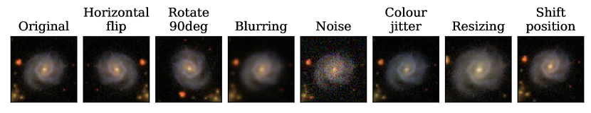
Figure 1: Common transformations used on galaxy imaging to produce positive pairs. From left to right: original $gri$-band composite, horizontal flip, rotation, blurring, noise addition, colour jitter, resizing and position shift.

In the next subsections we present the most commonly used loss functions applied to CL approaches and briefly review the most common NN architectures usually employed.

2.1 Contrastive loss

All CL frameworks share some version of the so-called contrastive loss function, which is generally optimized such that each positive pair is projected together in the representation space ${\boldsymbol{z}\in\mathbb{R}^{n}}$ and the negative pairs are repelled, although some of the latest proposed versions do not use negative pairs, as we discuss below.

The loss is calculated in the latent space of representations ${\boldsymbol{z}\in\mathbb{R}^{n}}$, which is the image of the trainable function $f$, where a pairwise distance metric $\langle\cdot,\cdot\rangle$ is defined. Given a set of representations ${\boldsymbol{z}\in\mathbb{R}^{n}}$, where each $\boldsymbol{z}$ has one identified positive pair $\boldsymbol{z}^{+}$ or more, the contrastive loss is a function that is minimized when the distance between positive pairs is minimized. The main difficulty is avoiding the trivial solution where all positive representations collapse into the same representation value. Several approaches have been proposed in the literature, which we briefly review now.

2.1.1 Spring loss

Chopra et al. (2005) and Hadsell et al. (2006) define a loss function that takes the pairwise Euclidean distance as metric. This resembles a spring system, where positive pairs of $\boldsymbol{z}_{i}$ are attracted, and the negative pairs that are within an $m$-distance of $\boldsymbol{z}_{i}$ are repelled. The introduction of negative pairs prevents the collapse into a trivial solution. This loss $L^{S}$ is defined pairwise for $\boldsymbol{z}_{i}$ and $\boldsymbol{z}_{j}$ as

$$L^{S}_{i,j}=Y\frac{1}{2}\langle\boldsymbol{z}_{i},\boldsymbol{z}_{j}\rangle^{2}+\frac{1}{2}(1-Y)\max{0,m-\langle\boldsymbol{z}_{i},\boldsymbol{z}_{j}\rangle},$$ (1)

where $Y$ is equal to one if $\boldsymbol{z}_{i}$ and $\boldsymbol{z}_{j}$ are identified as positive pairs, or zero if not. Therefore, either the left or right term in Eq.,1 is canceled, respectively.

2.1.2 Triplet loss

The triplet loss $L^{T}$ (Weinberger & Saul, 2009), who use a Mahalanobis distance metric (Chechik et al., 2010) with a bilinear model for the similarity measure, is similar to the spring loss, but each term is calculated considering three representations: the anchor ($i$), a positive ($i^{+}$), and a negative pair ($n$), as

$$L^{T}_{i,i^{+},n}=\max{0,\langle z_{i},z_{i}^{+}\rangle-\langle z_{i},z_{n}\rangle+d}.$$ (2)

Here, $d$ is a hyperparameter determining the distance between positive and negative pairs. This results in a more relaxed condition on the positive pairs than the Spring loss, as the latter attracts the positive pair to the same point in the representation space while repelling the negatives. In contrast, the Triplet loss only seeks to repel the negative representations a distance $d$ longer than the positive pairs, which favors repelling hard negatives.

2.1.3 Normalized cross entropy

Modern contrastive models are based on the noise-contrastive estimation (infoNCE) or normalized temperature-scaled cross entropy (NT-Xent) losses (Oord et al., 2018; Misra & van der Maaten, 2019; Chen et al., 2020a). It is generally defined element-wise as

$$L^{P}_{i}=-\log\frac{\exp(\langle\boldsymbol{z}_{i},\boldsymbol{z}i^{+}\rangle/h)}{\sum{k},,\exp(\langle\boldsymbol{z}_{i},\boldsymbol{z}_{k}\rangle/h)},$$ (3)

for the $i$-th object in the set, where $k$ iterates over all the representations $\boldsymbol{z}$ in the batch, and $\langle,,\rangle$ is a pairwise similarity measure, generally the cosine distance or a bilinear model. $h$ is a normalizing factor - temperature - that plays a similar role to $m$ in the previous approach, as it determines the concentration of the representation space by weighing the pairwise distances. This loss can be understood as a multiclass loss, where each representation’s correct class corresponds to its positive pair. The probability that a given object is assigned to its class over the other "wrong" classes is parameterized by the softmax function, and a cross-entropy loss is optimized.

As CL frameworks typically benefit from a large number of negative samples, the $L^{P}$ losses are more efficient (faster convergence) than the $L^{S}$ ones as every object accounts for the negative pairs of the object $\binom{N}{2}\times N$, while in the $L^{S}$ and $L^{T}$, only up to $\binom{N}{2}$ negative pairs are considered in total.

Some works have proposed losses based on mutual information (MI) maximization (Hjelm et al., 2019), where MI measures the dependence that a random variable $W$ has with another random variable $V$ and is defined as

$$I(w,v)=\mathbb{E}_{p(w,v)}\left[\log\frac{p(w,v)}{p(w)p(v)}\right].$$ (4)

While the MI-based approaches were proposed independently, the infoNCE optimization is analogous to the MI one, as the first is equivalent to maximizing a lower bound on MI (Oord et al. 2018).

2.1.4 Contrastive loss without negative pairs

More recently, Grill et al. (2020) proposed a loss that is calculated with the cosine distance between the positive pairs only and therefore departs from the standard CL setup:

$$L^{B}_{i}=2-2\frac{\langle\boldsymbol{z}_{i},\boldsymbol{z}_{i}^{+}\rangle}{||{z}_{i}||_{2}.||{z}_{i}^{+}||_{2}}$$ (5)

To avoid collapsing to the trivial solution, they use a twin network where one branch (target) is prevented to update its weights through back-propagation (Chen & He 2020). Instead, the weights of the target branch are a function of those in the symmetric branch (online) which has the same architecture (see Section 2.2 for more details)

In addition to these common augmentations, one of the most attractive properties of CL is the possibility to define custom augmentations which are domain-specific and allow one to marginalize over known nuisance effects. We will discuss this in more detail in sections 3 and 4.

2.2 Contrastive learning architectures

The representations $\boldsymbol{z}$ are computed using NNs. Over the past years, a number of frameworks have been developed, varying the structure and hyper-parameters of the NNs to obtain better performances.

Given that CL is primarily designed for datasets without labels, the evaluation and comparison of different approaches is not always straightforward. Architectures are therefore generally tested on standardized datasets for which labels do exist. The underlying idea to validate a new approach is that if extracted representations are meaningful, then a simple supervised classifier should be able to correctly classify the data. This way, the performance of the algorithms can be tested on supervised tasks, also known as downstream tasks. Therefore, when an approach is presented as more accurate than another in the literature, it generally refers to the accuracy in the downstream supervised task.

Although it is outside the scope of this brief overview to cover all existing implementations of CL, we attempt to summarize the major architecture conceptions that have resulted in significant performance improvements in downstream tasks in the following. A schematic view of these different architectures is presented in Figure 2.

2.2.1 CMC (Contrastive Multiview Coding)

Hadsell et al. (2006) stated that the representations benefit from a large number of negative examples. However, this comes at the computational cost of calculating an increasing number of loss terms and more representations in each learning step. This motivated following works to include a memory bank (Misra & van der Maaten 2019, Wu et al. 2018, Tian et al. 2019) that would store the representations calculated in previous iterations to increase the number of negative examples. In each iteration the loss is calculated considering the newly calculated representations in the mini-batch together with $m$ randomly sampled representations from the memory bank. This approach benefits from an adjustable number of negative examples without needing to compute more representations than those in the mini-batch.

2.2.2 MoCo (Momentum Contrastive)

Other implementations replace the memory bank with a parallel network that acts as a momentum encoder (MoCo, He et al. 2019), whose weights are updated as a moving average of the main branch’s weights. The momentum encoder calculates updated representations, which are later queued in a dictionary (a subset of the training set). The oldest representations in the dictionary are replaced by new ones as the network is trained. In contrast to the memory bank approach, the negative examples are sampled from the dictionary which is progressively updated. This prevents the network from using outdated representations from previous epochs as it is restricted to the representations of the immediately previous mini-batches as negative examples. He et al. (2019) found that this framework benefits from a slowly evolving momentum encoder to provide consistent representations over mini-batches and hypothesized that this is due to the rapidly changing main branch encoder.

2.2.3 SimCLR (Simple Contrastive Learning)

Chen et al. (2020a) propose a single Convolutional Neural Network (CNN) and no memory bank, so the negative examples are limited by the batch size. This sets a requirement on a minimum amount of memory for training. They show that this setup gets comparable results to the MoCo framework using large batch sizes (1024). Chen et al. (2020a) also prove that more parameters in the network, and more and stronger augmentations result in more accurate representations learned. Another important result of this work is that adding a set of fully connected layers before the loss calculation yields better representations in previous layers. This feature is then included in subsequent works (Chen et al. 2020b, Grill et al. 2020).

2.2.4 BYOL (Bootstrap Your Own Latent)

In the case of Grill et al. (2020) and Chen & He (2020), a set of twin networks is implemented. The networks’ architectures are identical on both branches except that one branch has an additional projection function. This is the branch where the back-propagation is implemented. The differences between the two implementations shed some light on understanding how these setups work. While BYOL’s target branch is progressively updated with the twin network’s weights to stabilize the output, SimSiam shares the weights in both branches. BYOL incorporates a set of fully connected layers after the CNN in both branches, although Chen & He (2020) claim that these layers do not improve the representations learned. However, both approaches agree on the need to limit the back-propagation to the online branch to avoid collapsing to a trivial solution, as the loss is calculated only with positive pairs (see subsection 2.1).

2.2.5 CLIP (Contrastive Language-Image Pre-training)

Recent architectures have started to use different types of networks for feature extraction, which are optimized for different data types. This allows for the combination of, for example, text and images. For example, Radford et al. (2021) train language and image encoders with a contrastive learning model to obtain representations of both inputs. They show that introducing descriptive text of an image in the CL setting produces better generalization and improves zero-shot learning.

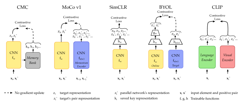
Figure 2: A reduced number of frameworks are shown in a simplified scheme to exemplify the variations of the Contrastive Learning framework zoo. On the left, Contrastive Multiview Coding (CMC, Tian et al. 2019) stores the representations computed in previous mini-batches in a memory bank to increase the number of negative examples. Although CMC proposes a twin network for comparing distinct versions of the input data, we represent in the figure only one branch to exemplify the memory bank setup. Second from the left, Momentum Contrastive (MoCo, He et al. 2019) has a parallel network that provides a queue of updated representations of negative examples. In the centre, Simple Contrastive Learning of visual Representations (SimCLR, Chen et al. 2020a) uses a unique CNN with a projection head ($h$) to compute the loss and extracts the final representations from the layer before $h$ after training. Second from the right, Boostrap Your Own Latent (BYOL, Grill et al. 2020) uses a parallel network to compute with the stop gradient operation on one branch to compute a positive pairs-only contrastive loss. On the right, Contrastive Language Image Pre-training (CLIP, Radford et al., 2021) trains simultaneously language and visual encoders to generate representations that match both domains.

3 Applications of contrastive learning in astronomy

Table 2 summarizes applications of deep CL to astrophysics so far. The first publications are from 2021, which illustrates the fact that the success of CL is relatively recent. Interestingly, the majority of the applications are in the field of galaxy formation. A possible explanation could be that there are large imaging datasets publicly and easily accessible.

Overall, CL is used either for pure data exploration - in which case it is usually followed by some sort of clustering - or to perform a downstream supervised classification or regression / inference using the representations obtained.

3.1 Inference from representations

3.1.1 Classification with limited amount of labels

Hayat et al. (2021) first applied the CL framework MoCo (see Figure 2 and Subsection 2.2) to a set of images from the SDSS I and II. They used the learned representations to perform two downstream tasks: galaxy morphology classification and photometric redshift estimation, as well as for data visualization. The work illustrated two main advantages of self-supervised CL. First, the authors showed the importance of using domain knowledge to obtain more robust representations. For example, they introduced custom augmentation to marginalize over reddening. As discussed in Section 2, CL easily allows for new augmentations to be included, making it a very flexible framework for representation learning. Second, Hayat et al. (2021) showed that when the representations are used for galaxy classification and photometric redshift estimation, one can achieve similar accuracies as with a pure supervised approach but with an order of magnitude fewer objects (Figure 3). This confirms that contrastive learning is helpful for reducing the volume of labeled datasets in astrophysics, as was demonstrated with natural images.

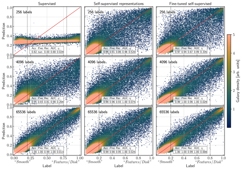
Figure 3: Application of contrastive learning (MoCo) to galaxy morphology classification by Hayat et al. (2021). The three columns show the classification performance in a supervised setting (left), a linear classifier directly on the self-supervised representations (center), and when fine-tuning the self-supervised encoder for a few epochs (right). $\eta$ measures the outlier fraction. While a pure supervised setting fails at providing meaningful morphology estimations with 256 examples (top left) a supervised model trained on the representations obtains significantly more accurate results (top middle).

A similar conclusion is reached by Slijepcevic et al. (2022) in an application to radio galaxy classification. By using the BYOL framework (see Figure 2 and subsection 2.2) they show that a classification based on the representations achieves comparable accuracy to a complete supervised approach. Lamdouar et al. (2022) explore the accuracy of CL for classifying time series of solar magnetic field measurements. They show again that CL is an efficient way of obtaining high classification accuracies when only limited labeled data is available (see also Mercea et al. (2023) for an extensive analysis of CL representations to classify seismic emissions in the solar surface).

3.1.2 Domain adaptation

Wei et al. (2022) also apply CL followed by a morphological classification downstream task, reaching similar conclusions, i.e., accuracies comparable to supervised classifications are reached but with a small amount of labels. Interestingly, they also show that the representations extracted with self-supervised learning generalize well to multiple imaging datasets. The concept of generalization to multiple tasks (i.e., domain adaptation and generalization) is an important property of CL. Domain adaptation with NNs generally refers to techniques used to improve the performance of a NN model trained on a source domain when applied to a different but related unlabeled target domain, by reducing the discrepancy between the two domains (see Li et al., 2021 for a review of the topic). Walmsley et al. (2022b) explore this in more detail for galaxy morphology applications. They use, in particular, what they call a hybrid contrastive-supervised approach to perform galaxy classifications from a set of visually classified galaxy images. This is performed by adding a supervised term to the BYOL framework, allowing for the performance of classifications while extracting representations that remain invariant to perturbations. They show that the representations learned by the hybrid approach can be efficiently fine-tuned with a few labels to perform supervised tasks for which no labels were provided. They apply this to find new ring galaxy candidates (Figure 4). In a more recent work, Ćiprijanović et al. (2023) also explore the concept of a universal domain adaptation approach for galaxy morphology. Instead of using a pure CL framework as the ones discussed in this review, they propose instead a custom approach based on an Adaptive Clustering loss (Saito et al., 2020; Li et al., 2021) on the latent representation. They test their approach by transferring a trained model from SDSS to the Dark Energy Camera Legacy Survey (DECaLS; Dey et al., 2019).

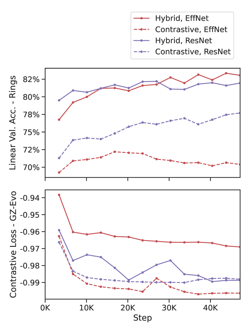
Figure 4: Performance of an hybrid CL approach to identify ring galaxies. The top and bottom panel show the accuracy and the evolution of the contrastive loss function of the downstream classification as a function of training steps. The hybrid CL/supervised approach reaches even higher accuracies than a pure CL one. Figure from Walmsley et al. (2022b).

3.1.3 Probabilistic inference

In addition to classification, CL representations can be employed as summary statistics for probabilistic inference. This is the case for example of the work by Shen et al. (2022) in which the CL representations are coupled to a Neural Density Estimator (Neural Flow) to estimate an approximate posterior distribution of physical properties of black hole mergers given the gravitational wave emission. In this case, using CL as conditioning for the Neural Flow has the advantage of improving the inference robustness to noise since the augmentations enable a marginalization over S/N.

3.2 Data visualization and clustering

Another set of applications is oriented towards data visualization and exploration. In these cases, a specific downstream task is not sought, but the main purpose of the representations is to explore and find patterns in the data. In that respect, it is closer to a purely unsupervised application.

Sarmiento et al. (2021), for example, use SimCLR (see Figure 2 and Subsection 2.2) to extract meaningful representations of inferred stellar population and kinematic maps for $\sim 10,000$ galaxies in the Mapping Nearby Galaxies at Apache Point Observatory (MaNGA; Bundy et al., 2015; Abdurro’uf et al., 2022) survey. They show that the contrastive framework naturally orders galaxies based on their physical properties without supervision and rediscovers some well-known relations with a purely data-driven approach. Interestingly, they also find that, for that particular case, other representation learning strategies such as PCA fail to extract physical properties and focus more on instrumental effects. The flexibility of contrastive learning to include custom domain-driven augmentations is key to obtain more physical representations (Figure 5). More recently,Vega-Ferrero et al. (2023) has applied a similar approach to images of galaxies from the Cosmic Evolution Early Release Science survey (CEERS,Finkelstein et al., 2022). By introducing an augmentation that goes from a noiseless to a noisy version of images, they show that the CL representations offer a morphological description that becomes robust to noise, a property lacking in most previous morphology classifications.

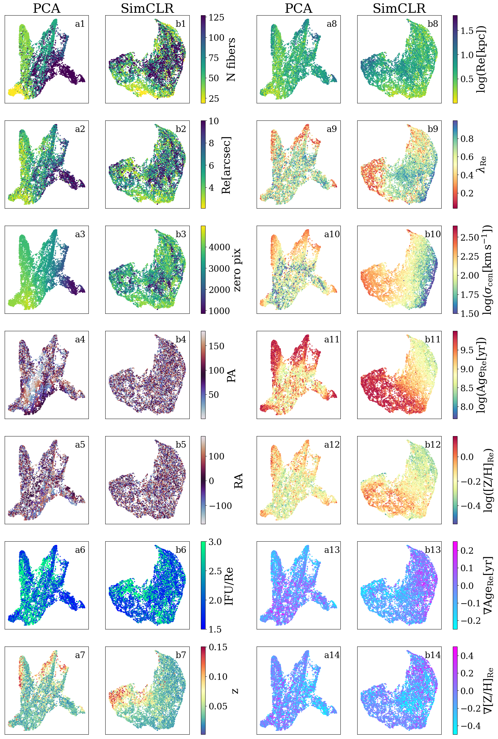
Figure 5: Application of contrastive learning (SimCLR) for data visualization and clustering from Sarmiento et al. (2021). The different panels show a UMAP projection of PCA and SimCLR representations color coded by instrumental and other nuisance parameters (leftmost columns) and physical properties (rightmost columns). While PCA capture mostly instrumental effects, the CL representation are able to marginalize over those.

Guo et al. (2022) use a similar contrastive-learning (BYOL) followed by clustering applied to galaxy images in the far-infrared from the Wide-field Infrared Survey Explorer (WISE) survey (Wright et al., 2010). They demonstrate that the method successfully organizes objects based on similarity and discuss the properties for the different obtained clusters. The work does not, however, discuss the advantages of CL over other representation learning settings in this particular case.

3.3 Similarity search and anomaly detection

Two straightforward applications of robust representations are similarity search and anomaly detection. Given that CL representations, by construction, are similar for objects with similar properties - marginalized over the nuisance properties encoded in the augmentations - one can query the representations to look for similar data or for isolated objects. Stein et al. (2021) demonstrate efficient similarity search using CL representations, as illustrated in Figure 6 where the model is queried to identify galaxy images with similar properties.

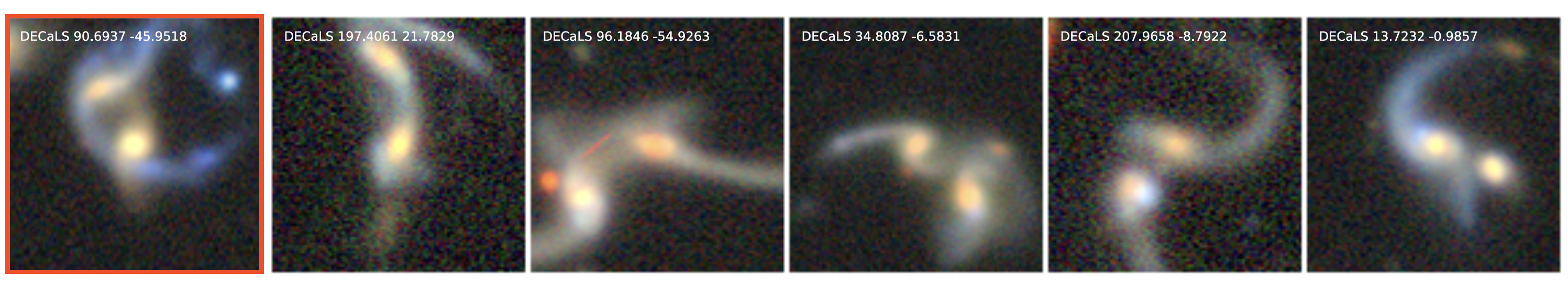
Figure 6: Application of contrastive learning for similarity search of galaxy images with similar morphological features. The leftmost image shows a galaxy candidate and the others are similar image candidates based on the representations. Figure adapted from Stein et al. (2021)

.

3.4 Other applications

Recent work by Doorenbos et al. (2022) uses CL for a different purpose: generating galaxy spectra from images. This illustrates how meaningful representations can be used for a wide number of applications and shows a possible evolution for the near future. The authors use a conditional diffusion model (e.g., Chen et al., 2021) to generate possible candidates of spectra given an image of a galaxy. Diffusion models are a class of generative models that learn the dynamics of how a distribution evolves over time by iteratively applying a diffusion process to a simple initial distribution, making them well-suited for tasks such as density estimation, generative modeling, and image synthesis (see the introduction section for more references on this type of generative models). Then they use CL to find common representations of real spectra and their corresponding images. Among all candidates resulting from the sampling of the diffusion model, the best candidate is selected by identifying the spectrum producing the closest CL representation to the target image (Figure 7). In addition to the specific application, which is potentially interesting for data exploration, this work illustrates the unique capability of CL to obtain simultaneous representations of heterogeneous data such as spectra and images.

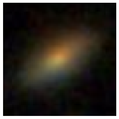
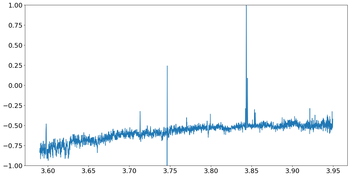
Figure 7: Application of contrastive learning for spectra generation from images. The leftmost column shows the image from SDSS for which a spectrum is predicted. The middle column shows the target spectrum and the rightmost one shows the best candidate according to CL. Figure adapted from Doorenbos et al. (2022).

Table 2: CL applied to astrophysics

Article	Astronomy field	Data	Based on	Downstream task
Hayat et al. (2021)	Galaxies	Photometric Imaging	MoCo	Regression (photo-z, morphology)
		(SDSS)	He et al. (2019)
Sarmiento et al. (2021)	Galaxies	Integral Field Spectroscopy	SimCLR	Clustering
		(MaNGA)	Chen et al. (2020a)
Stein et al. (2021)	Galaxies	Photometric Imaging	MoCo	Similarity search
		(DESI Legacy Imaging Survey)	He et al. (2019)
Walmsley et al. (2022b)	Galaxies	Photometric Imaging	BYOL (loss)	Transfer Learning
			Grill et al. (2020)
Slijepcevic et al. (2022)	Galaxies		BYOL	Morphology classification of radio galaxies
			Grill et al. (2020)
Wei et al. (2022)	Galaxies	Photometric Imaging	SimCLR	Morphology classification
		SDSS	Chen et al. (2020a)
Shen et al. (2022)	Gravitational Waves	surrogate waveforms	SimCLR (NT-Xent loss)	Regression (masses, spin, quasinormal modes)
		simulations + LIGO	Chen et al. (2020a)
Doorenbos et al. (2022)	Galaxies	Photometric Imaging and Spectra	SimCLR (NT-Xent loss)	Predict spectra from images (combined with multimodal conditional diffusion models)
		(SDSS)	Chen et al. (2020a)
Lamdouar et al. (2022)	Solar		(Triplet loss)
Guo et al. (2022)	Galaxies	Photometric Imaging	BYOL	Clustering
		(WISE)	Grill et al. (2020)
Mercea et al. (2023)	Solar	Photospheric Dopplergram maps	SimCLR& SupCon	Classification (sunquake detection)
		Michelson Doppler Imager	Chen et al. (2020a)
		Helioseismic and Magnetic Imager	Khosla et al. (2020)
Vega-Ferrero et al. (2023)	Galaxies	Photometric Imaging	SimCLR	Domain adaptation and Clustering
		JWST and TNG50 simulations	Chen et al. (2020a)
Ćiprijanović et al. (2023)	Galaxies	Photometric Imaging	Adaptive Clustering	Domain adaptation and Clustering
		SDSS and DECaLS

4 Discussion

CL has emerged as an efficient approach for representation learning over the past years with some successful applications in astronomy as described in the previous section. We discuss in the following some practical considerations for non-expert readers interested in using CL methods for other astrophysical problems.

4.1 What is contrastive learning useful for?

CL has been shown to be primarily a promising way to address the issue of the lack of labeled data for supervised classification and inference.

Over the past few years, deep learning applications have become more frequent in astronomy, with supervised approaches still being the most common (e.g.,Huertas-Company & Lanusse, 2023). One of the main bottlenecks of such applications is the availability of labeled data. The vast majority of astronomical data is unlabeled, limiting the applicability of ML for classification or inference. In this context, the community needs methods that can work on small datasets when only a limited amount of labels is available or that can generalize well across domains and, therefore, be applied to different datasets (see e.g., Ćiprijanović et al., 2023). From the few works exploring CL in astronomy, it appears as a promising approach to at least partially solve some of these issues. For instance,Hayat et al. (2021) have shown that CL can reduce the number of required labels for supervised classification and regression by an order of magnitude. Along the same lines,Walmsley et al. (2022b) have shown that adding a CL component seems to be a promising avenue towards general "foundation" models for morphology classification, i.e., models that can be applied to a variety of different datasets. In addition to being a feature extraction method for supervised downstream tasks, CL can also be used alone as a visualization/exploratory tool (see e.g.,Sarmiento et al., 2021; Stein et al., 2021). Although there are various techniques for representation learning (see the introduction) and for transferring trained models (see e.g.,Domínguez Sánchez et al., 2019; Ćiprijanović et al., 2020), CL has unique properties that make it particularly useful for astrophysics.

Arguably, the main advantage of CL is that, unlike other approaches, it does not have a predefined encoded metric, allowing it to be adapted for every application using domain knowledge. The similarity pretext task that CL solves is determined by the augmentations, which defines the positive pairs. In that respect, although there are some standard augmentations that can be used for imaging applications (see Figure 1), CL has room for domain-specific augmentations. This allows one to introduce domain knowledge in the representations without explicitly defining a metric. This is particularly relevant for astrophysics, in which there usually exist selection and instrumental effects that are known and fairly easy to model, but can potentially bias other representation learning algorithms with a fixed metric. CL enables a relatively straightforward marginalization over these nuisance parameters. Several works have already shown the advantages of using domain-specific augmentation. Mercea et al. (2023) discuss the use of different transformations on regression power maps derived from solar photospheric dopplergrams. They use time-based mixing (stacking of subsequent maps), a low-pass filter followed by solarization, and random erasing of signals. Sarmiento et al. (2021) use specific observational effects from the MaNGA survey, while Abul Hayat et al. (2021) include reddening as part of the augmentation sets. Generally speaking, any dataset affected by known nuisance effects that can be modeled might potentially be a good candidate for application of CL.

Another important consequence of the flexibility of CL for defining the similarity metric is that it opens the door for obtaining representations of different data types. There are a number of recent successful applications of CL in the ML community combining speech and images, for example (e.g., Ramesh et al., 2021). In astronomy, it is potentially an interesting avenue to extract simultaneous information from images and spectra, a task that is difficult to achieve with other approaches. The first work to have explored this, to our knowledge, is the one by Doorenbos et al. (2022), with encouraging results that open new, interesting research avenues.

4.2 What is contrastive learning not useful for?

It is important to emphasize that CL is not particularly efficient as a dimensionality reduction algorithm. In fact, several works have shown that increasing the dimensionality of the representation space generally results in an improved performance (e.g.,Chen et al., 2020a; Sarmiento et al., 2021). As a result, the obtained representations are still of fairly high dimension and not easy to visualize. This is why several authors have coupled the resulting representations with a pure dimensionality reduction algorithm for visualization purposes (see e.g. Hayat et al., 2021). Therefore CL is not the approach to use for inferring the true dimensionality of a dataset. In fact, unlike PCA, there are no constraints on the representations obtained and therefore it is always the case that the different representations are highly correlated.

This also implies a more challenging interpretability of the extracted features compared to other representation learning algorithms. Both the high dimensionality and the correlation between features significantly complicate the task of physically interpreting the extracted representations. CL is probably not the preferred approach for gaining physical insight by exploring the representations. However, CL frameworks can be coupled with other methods to increase interpretability. One could also potentially add regularization terms into the loss functions to penalize strong correlations in the latent space.

5 Summary and Conclusions

This work briefly reviews contrastive methods for representation learning and their application to astrophysics. CL is a self-supervised learning method which obtains meaningful representations of high-dimensionality datasets by solving a similarity pretext task. Compared to other representation learning techniques, the similarity metric is not encoded but is defined through augmentations of the input dataset. By defining positive pairs as the set of all augmented versions of the same data point, the representations become invariant to such transformations.

We review a dozen existing works using CL in astrophysics, the vast majority in the field of galaxy formation. Applications are roughly divided in two main families: downstream regression, inference and classification; and data exploration. From these works, we conclude that CL is as a powerful method to train supervised algorithms with a limited amount of labels. The flexibility of the augmentations allowing domain-specific perturbations makes CL a suitable method for marginalizing over known instrumental or other nuisance effects which can be modeled in astronomy. An interesting avenue for the future, which is also enabled by CL and has just started to be explored in astrophysics, is the combinations of different data types such as imaging and spectra.

Data Availability

No data are used in this review work.

References

- Abazajian et al. (2009) Abazajian, K. N., Adelman-McCarthy, J. K., Agüeros, M. A., Allam, S. S., Allende Prieto, C., An, D., Anderson, K. S. J., Anderson, S. F., Annis, J., Bahcall, N. A., Bailer-Jones, C. A. L., Barentine, J. C., Bassett, B. A., Becker, A. C., Beers, T. C., Bell, E. F., Belokurov, V., Berlind, A. A., Berman, E. F., Bernardi, M., Bickerton, S. J., Bizyaev, D., Blakeslee, J. P., Blanton, M. R., Bochanski, J. J., Boroski, W. N., Brewington, H. J., Brinchmann, J., Brinkmann, J., Brunner, R. J., Budavári, T., Carey, L. N., Carliles, S., Carr, M. A., Castander, F. J., Cinabro, D., Connolly, A. J., Csabai, I., Cunha, C. E., Czarapata, P. C., Davenport, J. R. A., de Haas, E., Dilday, B., Doi, M., Eisenstein, D. J., Evans, M. L., Evans, N. W., Fan, X., Friedman, S. D., Frieman, J. A., Fukugita, M., Gänsicke, B. T., Gates, E., Gillespie, B., Gilmore, G., Gonzalez, B., Gonzalez, C. F., Grebel, E. K., Gunn, J. E., Györy, Z., Hall, P. B., Harding, P., Harris, F. H., Harvanek, M., Hawley, S. L., Hayes, J. J. E., Heckman, T. M., Hendry, J. S., Hennessy, G. S., Hindsley, R. B., Hoblitt, J., Hogan, C. J., Hogg, D. W., Holtzman, J. A., Hyde, J. B., Ichikawa, S.-i., Ichikawa, T., Im, M., Ivezić, Ž., Jester, S., Jiang, L., Johnson, J. A., Jorgensen, A. M., Jurić, M., Kent, S. M., Kessler, R., Kleinman, S. J., Knapp, G. R., Konishi, K., Kron, R. G., Krzesinski, J., Kuropatkin, N., Lampeitl, H., Lebedeva, S., Lee, M. G., Lee, Y. S., French Leger, R., Lépine, S., Li, N., Lima, M., Lin, H., Long, D. C., Loomis, C. P., Loveday, J., Lupton, R. H., Magnier, E., Malanushenko, O., Malanushenko, V., Mandelbaum, R., Margon, B., Marriner, J. P., Martínez-Delgado, D., Matsubara, T., McGehee, P. M., McKay, T. A., Meiksin, A., Morrison, H. L., Mullally, F., Munn, J. A., Murphy, T., Nash, T., Nebot, A., Neilsen, Eric H., J., Newberg, H. J., Newman, P. R., Nichol, R. C., Nicinski, T., Nieto-Santisteban, M., Nitta, A., Okamura, S., Oravetz, D. J., Ostriker, J. P., Owen, R., Padmanabhan, N., Pan, K., Park, C., Pauls, G., Peoples, John, J., Percival, W. J., Pier, J. R., Pope, A. C., Pourbaix, D., Price, P. A., Purger, N., Quinn, T., Raddick, M. J., Re Fiorentin, P., Richards, G. T., Richmond, M. W., Riess, A. G., Rix, H.-W., Rockosi, C. M., Sako, M., Schlegel, D. J., Schneider, D. P., Scholz, R.-D., Schreiber, M. R., Schwope, A. D., Seljak, U., Sesar, B., Sheldon, E., Shimasaku, K., Sibley, V. C., Simmons, A. E., Sivarani, T., Allyn Smith, J., Smith, M. C., Smolčić, V., Snedden, S. A., Stebbins, A., Steinmetz, M., Stoughton, C., Strauss, M. A., SubbaRao, M., Suto, Y., Szalay, A. S., Szapudi, I., Szkody, P., Tanaka, M., Tegmark, M., Teodoro, L. F. A., Thakar, A. R., Tremonti, C. A., Tucker, D. L., Uomoto, A., Vanden Berk, D. E., Vandenberg, J., Vidrih, S., Vogeley, M. S., Voges, W., Vogt, N. P., Wadadekar, Y., Watters, S., Weinberg, D. H., West, A. A., White, S. D. M., Wilhite, B. C., Wonders, A. C., Yanny, B., Yocum, D. R., York, D. G., Zehavi, I., Zibetti, S., & Zucker, D. B., 2009. The Seventh Data Release of the Sloan Digital Sky Survey, ApJS, 182(2), 543–558.
- Abdurro’uf et al. (2022) Abdurro’uf, Accetta, K., Aerts, C., Silva Aguirre, V., Ahumada, R., Ajgaonkar, N., Filiz Ak, N., Alam, S., Allende Prieto, C., Almeida, A., Anders, F., Anderson, S. F., Andrews, B. H., Anguiano, B., Aquino-Ortíz, E., Aragón-Salamanca, A., Argudo-Fernández, M., Ata, M., Aubert, M., Avila-Reese, V., Badenes, C., Barbá, R. H., Barger, K., Barrera-Ballesteros, J. K., Beaton, R. L., Beers, T. C., Belfiore, F., Bender, C. F., Bernardi, M., Bershady, M. A., Beutler, F., Bidin, C. M., Bird, J. C., Bizyaev, D., Blanc, G. A., Blanton, M. R., Boardman, N. F., Bolton, A. S., Boquien, M., Borissova, J., Bovy, J., Brandt, W. N., Brown, J., Brownstein, J. R., Brusa, M., Buchner, J., Bundy, K., Burchett, J. N., Bureau, M., Burgasser, A., Cabang, T. K., Campbell, S., Cappellari, M., Carlberg, J. K., Wanderley, F. C., Carrera, R., Cash, J., Chen, Y.-P., Chen, W.-H., Cherinka, B., Chiappini, C., Choi, P. D., Chojnowski, S. D., Chung, H., Clerc, N., Cohen, R. E., Comerford, J. M., Comparat, J., da Costa, L., Covey, K., Crane, J. D., Cruz-Gonzalez, I., Culhane, C., Cunha, K., Dai, Y. S., Damke, G., Darling, J., Davidson, James W., J., Davies, R., Dawson, K., De Lee, N., Diamond-Stanic, A. M., Cano-Díaz, M., Sánchez, H. D., Donor, J., Duckworth, C., Dwelly, T., Eisenstein, D. J., Elsworth, Y. P., Emsellem, E., Eracleous, M., Escoffier, S., Fan, X., Farr, E., Feng, S., Fernández-Trincado, J. G., Feuillet, D., Filipp, A., Fillingham, S. P., Frinchaboy, P. M., Fromenteau, S., Galbany, L., García, R. A., García-Hernández, D. A., Ge, J., Geisler, D., Gelfand, J., Géron, T., Gibson, B. J., Goddy, J., Godoy-Rivera, D., Grabowski, K., Green, P. J., Greener, M., Grier, C. J., Griffith, E., Guo, H., Guy, J., Hadjara, M., Harding, P., Hasselquist, S., Hayes, C. R., Hearty, F., Hernández, J., Hill, L., Hogg, D. W., Holtzman, J. A., Horta, D., Hsieh, B.-C., Hsu, C.-H., Hsu, Y.-H., Huber, D., Huertas-Company, M., Hutchinson, B., Hwang, H. S., Ibarra-Medel, H. J., Chitham, J. I., Ilha, G. S., Imig, J., Jaekle, W., Jayasinghe, T., Ji, X., Johnson, J. A., Jones, A., Jönsson, H., Katkov, I., Khalatyan, Arman, D., Kinemuchi, K., Kisku, S., Knapen, J. H., Kneib, J.-P., Kollmeier, J. A., Kong, M., Kounkel, M., Kreckel, K., Krishnarao, D., Lacerna, I., Lane, R. R., Langgin, R., Lavender, R., Law, D. R., Lazarz, D., Leung, H. W., Leung, H.-H., Lewis, H. M., Li, C., Li, R., Lian, J., Liang, F.-H., Lin, L., Lin, Y.-T., Lin, S., Lintott, C., Long, D., Longa-Peña, P., López-Cobá, C., Lu, S., Lundgren, B. F., Luo, Y., Mackereth, J. T., de la Macorra, A., Mahadevan, S., Majewski, S. R., Manchado, A., Mandeville, T., Maraston, C., Margalef-Bentabol, B., Masseron, T., Masters, K. L., Mathur, S., McDermid, R. M., Mckay, M., Merloni, A., Merrifield, M., Meszaros, S., Miglio, A., Di Mille, F., Minniti, D., Minsley, R., Monachesi, A., Moon, J., Mosser, B., Mulchaey, J., Muna, D., Muñoz, R. R., Myers, A. D., Myers, N., Nadathur, S., Nair, P., Nandra, K., Neumann, J., Newman, J. A., Nidever, D. L., Nikakhtar, F., Nitschelm, C., O’Connell, J. E., Garma-Oehmichen, L., Luan Souza de Oliveira, G., Olney, R., Oravetz, D., Ortigoza-Urdaneta, M., Osorio, Y., Otter, J., Pace, Z. J., Padilla, N., Pan, K., Pan, H.-A., Parikh, T., Parker, J., Peirani, S., Peña Ramírez, K., Penny, S., Percival, W. J., Perez-Fournon, I., Pinsonneault, M., Poidevin, F., Poovelil, V. J., Price-Whelan, A. M., Bárbara de Andrade Queiroz, A., Raddick, M. J., Ray, A., Rembold, S. B., Riddle, N., Riffel, R. A., Riffel, R., Rix, H.-W., Robin, A. C., Rodríguez-Puebla, A., Roman-Lopes, A., Román-Zúñiga, C., Rose, B., Ross, A. J., Rossi, G., Rubin, K. H. R., Salvato, M., Sánchez, S. F., Sánchez-Gallego, J. R., Sanderson, R., Santana Rojas, F. A., Sarceno, E., Sarmiento, R., Sayres, C., Sazonova, E., Schaefer, A. L., Schiavon, R., Schlegel, D. J., Schneider, D. P., Schultheis, M., Schwope, A., Serenelli, A., Serna, J., Shao, Z., Shapiro, G., Sharma, A., Shen, Y., Shetrone, M., Shu, Y., Simon, J. D., Skrutskie, M. F., Smethurst, R., Smith, V., Sobeck, J., Spoo, T., Sprague, D., Stark, D. V., Stassun, K. G., Steinmetz, M., Stello, D., Stone-Martinez, A., Storchi-Bergmann, T., Stringfellow, G. S., Stutz, A., Su, Y.-C., Taghizadeh-Popp, M., Talbot, M. S., Tayar, J., Telles, E., Teske, J., Thakar, A., Theissen, C., Tkachenko, A., Thomas, D., Tojeiro, R., Hernandez Toledo, H., Troup, N. W., Trump, J. R., Trussler, J., Turner, J., Tuttle, S., Unda-Sanzana, E., Vázquez-Mata, J. A., Valentini, M., Valenzuela, O., Vargas-González, J., Vargas-Magaña, M., Alfaro, P. V., Villanova, S., Vincenzo, F., Wake, D., Warfield, J. T., Washington, J. D., Weaver, B. A., Weijmans, A.-M., Weinberg, D. H., Weiss, A., Westfall, K. B., Wild, V., Wilde, M. C., Wilson, J. C., Wilson, R. F., Wilson, M., Wolf, J., Wood-Vasey, W. M., Yan, R., Zamora, O., Zasowski, G., Zhang, K., Zhao, C., Zheng, Z., Zheng, Z., & Zhu, K., 2022. The Seventeenth Data Release of the Sloan Digital Sky Surveys: Complete Release of MaNGA, MaStar, and APOGEE-2 Data, ApJS, 259(2), 35.
- Abul Hayat et al. (2021) Abul Hayat, M., Harrington, P., Stein, G., Lukić, Z., & Mustafa, M., 2021. Estimating Galactic Distances From Images Using Self-supervised Representation Learning, arXiv e-prints, p. arXiv:2101.04293.
- Arjovsky et al. (2017) Arjovsky, M., Chintala, S., & Bottou, L., 2017. Wasserstein gan, arXiv preprint arXiv:1701.07875.
- Belkin & Niyogi (2003) Belkin, M. & Niyogi, P., 2003. Laplacian eigenmaps for dimensionality reduction and data representation, Neural Computation, 15, 1373–1396.
- Bengio et al. (2013) Bengio, Y., Courville, A., & Vincent, P., 2013. Representation learning: A review and new perspectives, IEEE transactions on pattern analysis and machine intelligence, 35(8), 1798–1828.
- Biehl (2022) Biehl, M., 2022. The Shallow and the Deep: A biased introduction to neural networks and old school machine learning, Rijksuniversiteit Groningen.
- Bishop (2006) Bishop, C. M., 2006. Pattern recognition and machine learning, Springer.
- Brock et al. (2018) Brock, A., Donahue, J., & Simonyan, K., 2018. Large scale gan training for high fidelity natural image synthesis, in International Conference on Learning Representations.
- Bundy et al. (2015) Bundy, K., Bershady, M. A., Law, D. R., Yan, R., Drory, N., MacDonald, N., Wake, D. A., Cherinka, B., Sánchez-Gallego, J. R., Weijmans, A.-M., Thomas, D., Tremonti, C., Masters, K., Coccato, L., Diamond-Stanic, A. M., Aragón-Salamanca, A., Avila-Reese, V., Badenes, C., Falcón-Barroso, J., Belfiore, F., Bizyaev, D., Blanc, G. A., Bland-Hawthorn, J., Blanton, M. R., Brownstein, J. R., Byler, N., Cappellari, M., Conroy, C., Dutton, A. A., Emsellem, E., Etherington, J., Frinchaboy, P. M., Fu, H., Gunn, J. E., Harding, P., Johnston, E. J., Kauffmann, G., Kinemuchi, K., Klaene, M. A., Knapen, J. H., Leauthaud, A., Li, C., Lin, L., Maiolino, R., Malanushenko, V., Malanushenko, E., Mao, S., Maraston, C., McDermid, R. M., Merrifield, M. R., Nichol, R. C., Oravetz, D., Pan, K., Parejko, J. K., Sanchez, S. F., Schlegel, D., Simmons, A., Steele, O., Steinmetz, M., Thanjavur, K., Thompson, B. A., Tinker, J. L., van den Bosch, R. C. E., Westfall, K. B., Wilkinson, D., Wright, S., Xiao, T., & Zhang, K., 2015. Overview of the SDSS-IV MaNGA Survey: Mapping nearby Galaxies at Apache Point Observatory, ApJ, 798(1), 7.
- Chechik et al. (2010) Chechik, G., Sharma, V., Shalit, U., & Bengio, S., 2010. Large scale online learning of image similarity through ranking, Journal of Machine Learning Research, 11(36), 1109–1135.
- Chen et al. (2018a) Chen, R. T., Li, X., Grosse, R. B., & Duvenaud, D. K., 2018a. Isolating sources of disentanglement in variational autoencoders, in Advances in Neural Information Processing Systems, pp. 7512–7523.
- Chen et al. (2018b) Chen, R. T., Rubanova, Y., Bettencourt, J., & Duvenaud, D., 2018b. Neural ordinary differential equations, in Advances in Neural Information Processing Systems, pp. 6571–6583.
- Chen et al. (2021) Chen, R. T., Fan, J., Agrawal, S., & Duvenaud, D., 2021. Conditional diffusion models for continuous and discrete outcomes, in International Conference on Machine Learning, pp. 1716–1726.
- Chen et al. (2020a) Chen, T., Kornblith, S., Norouzi, M., & Hinton, G., 2020a. A simple framework for contrastive learning of visual representations.
- Chen & He (2020) Chen, X. & He, K., 2020. Exploring simple siamese representation learning.
- Chen et al. (2020b) Chen, X., Fan, H., Girshick, R., & He, K., 2020b. Improved baselines with momentum contrastive learning.
- Chen & Bach (2021) Chen, X.-J. & Bach, F., 2021. Stochastic differential equations as diffusions: Reinterpreting flow models as continuous-time markov chains, International Conference on Learning Representations.
- Chopra et al. (2005) Chopra, S., Hadsell, R., & LeCun, Y., 2005. Learning a similarity metric discriminatively, with application to face verification, in 2005 IEEE Computer Society Conference on Computer Vision and Pattern Recognition (CVPR’05), vol. 1, pp. 539–546 vol. 1.
- Ćiprijanović et al. (2020) Ćiprijanović, A., Snyder, G. F., Nord, B., & Peek, J. E. G., 2020. DeepMerge: Classifying high-redshift merging galaxies with deep neural networks, Astronomy and Computing, 32, 100390.