Monte Carlo inference for semiparametric Bayesian regression

Abstract

Data transformations are essential for broad applicability of parametric regression models. However, for Bayesian analysis, joint inference of the transformation and model parameters typically involves restrictive parametric transformations or nonparametric representations that are computationally inefficient and cumbersome for implementation and theoretical analysis, which limits their usability in practice. This paper introduces a simple, general, and efficient strategy for joint posterior inference of an unknown transformation and all regression model parameters. The proposed approach directly targets the posterior distribution of the transformation by linking it with the marginal distributions of the independent and dependent variables, and then deploys a Bayesian nonparametric model via the Bayesian bootstrap. Crucially, this approach delivers (1) joint posterior consistency under general conditions, including multiple model misspecifications, and (2) efficient Monte Carlo (not Markov chain Monte Carlo) inference for the transformation and all parameters for important special cases. These tools apply across a variety of data domains, including real-valued, integer-valued, compactly-supported, and positive data. Simulation studies and an empirical application demonstrate the effectiveness and efficiency of this strategy for semiparametric Bayesian analysis with linear models, quantile regression, and Gaussian processes.

Keywords: Bayesian nonparametrics; Gaussian processes; Nonlinear regression; Quantile regression; Transformations.

1 Introduction

Transformations are widely useful for statistical modeling and data analysis. A well-chosen or learned transformation can significantly enhance the applicability of fundamental statistical modeling frameworks, such as Gaussian models (Box and Cox,, 1964), linear and nonlinear regression models (Ramsay,, 1988; Carroll and Ruppert,, 1988), survival analysis (Cheng et al.,, 1995), discriminant analysis (Lin and Jeon,, 2003), and graphical models (Liu et al.,, 2009), among many other examples. This is especially true for data with complex marginal features, such multimodality, skewness, zero-inflation, and discrete or compact support, and for Bayesian probability models that must adapt to these features.

Consider the transformed regression model for paired data $\mathcal{D}_{n}=\{(x_{i},y_{i})\}_{i=1}^{n}$ with $x_{i}\in\mathcal{X}\subseteq\mathbb{R}^{d}$ and $y_{i}\in\mathcal{Y}\subseteq\mathbb{R}$:

$$g(y_{i}) =z_{i}$$ (1)

$$z_{i} \stackrel{{\scriptstyle indep}}{{\sim}}P_{Z\mid\theta,X=x_{i}}$$ (2)

where $g:\mathcal{Y}\to\mathbb{R}$ is a monotone increasing transformation and $P_{Z\mid\theta,X}$ is a covariate-dependent and continuous distribution with parameters $\theta\in\Theta\subseteq\mathbb{R}^{p}$. Informally, $P_{Z\mid\theta,X}$ may be considered the core statistical model, while the transformation $g$ serves to potentially improve the adequacy of this model for the given data $\mathcal{D}_{n}$. When the transformation is unknown and $P_{Z\mid\theta,X}$ is a parametric model, then (1)–(2) is a semiparametric regression model. Identifiability will be imposed on $P_{Z\mid\theta,X}$, typically by fixing the location and scale, and is discussed subsequently.

We focus on Bayesian analysis of (1)–(2), but acknowledge the rich history of frequentist inference for transformation models, including monotone stress minimization (Kruskal,, 1965) alternating conditional expectations (Breiman and Friedman,, 1985), additivity and variance stabilization (Tibshirani,, 1988), transnormal regression models (Fan et al.,, 2016), and many others.

There are various important examples of (1)–(2):

Example 1.

Consider the general regression model

$$z_{i}=f_{\theta}(x_{i})+\sigma\epsilon_{i}$$ (3)

where $f_{\theta}$ is parametrized by $\theta\in\Theta\subseteq\mathbb{R}^{p}$. Typically, the errors are $\epsilon_{i}\stackrel{{\scriptstyle iid}}{{\sim}}N(0,1)$ and thus $P_{Z\mid\theta,X=x_{i}}=N(f_{\theta}(x_{i}),\sigma^{2})$. Although this model may be applied directly to $y$ and offers flexibility via $f_{\theta}$, the Gaussian assumption for the errors is often restrictive and inadequate. The modeler must then consider whether to revise $f_{\theta}$, specify an alternative distribution for $\epsilon_{i}$, or incorporate a transformation via (1). We explore the latter option, and seek to provide excellent empirical performance, efficient algorithms, and strong theoretical guarantees for Bayesian inference.

Example 2.

Bayesian quantile regression specifies an error distribution for (3) such that $f_{\theta}(x)$ target the $\tau$th quantile of $P_{Z\mid\theta,X}$. The most common choice is the asymmetric Laplace distribution (ALD) with density $p_{\tau}(\epsilon)=\tau(1-\tau)\exp\{-\rho_{\tau}(\epsilon)\}$ and $\rho_{\tau}(\epsilon)=\epsilon\{\tau-I(\epsilon<0)\}$ is the check loss function (Yu and Moyeed,, 2001). However, the ALD is often a poor model for data, especially when $\tau$ is close to zero or one (see Section 3.2). A transformation can alleviate such inadequacy. The $\tau$th quantile of $z$ corresponds to the $g^{-1}(\tau)$th quantile of $y$, so $f_{\theta}(x)$ maintains interpretability and the transformed regression model readily provides quantile estimates for $y$ at $x$.

Example 3.

In survival analysis, it is common to express a time-to-event variable $y_{i}>0$ in the form of (1)–(3), referred to as a (linear) transformation model (Cheng et al.,, 1995; Chen et al.,, 2002; Mallick and Walker,, 2003). Specific modifications of (3) with $f_{\theta}(x)=-x^{\mathrm{\scriptscriptstyle T}}\theta$ and $\sigma=1$ produce popular semiparametric models. First, the proportional hazards model uses subject-specific hazard function $\lambda_{i}(t)=\lambda_{0}(t)\exp(x_{i}^{\mathrm{\scriptscriptstyle T}}\theta),$ where $\lambda_{0}$ is the (nonparametric) baseline hazard function and $S_{0}(t)=\exp\{-\int_{t}^{\infty}\lambda_{0}(r)\ dr\}$ is the baseline survival function. The proportional hazards model is obtained from (3) when $\epsilon_{i}$ follows the extreme-value distribution, $p(\epsilon)=\exp(\epsilon)\exp\{-\exp(\epsilon)\}$, while the transformation is linked to the baseline functions via $g(t)=\log[-\log\{S_{0}(t)\}]=\log\int_{0}^{t}\lambda_{0}(r)$. Alternatively, the proportional odds model uses the subject-specific odds function $\omega_{i}(t)=\mbox{pr}(y_{i}\leq t)\{1-\mbox{pr}(y_{i}\leq t)\}^{-1}=\omega_{0}(t)\exp(-x_{i}^{\mathrm{\scriptscriptstyle T}}\theta)$, where $\omega_{0}$ is the (nonparametric) baseline odds function. This model is obtained from (3) when $\epsilon_{i}$ follows the standard logistic distribution, $p(\epsilon)=\exp(-\epsilon)\{1+\exp(-\epsilon)\}^{-2}$, and the transformation is $g(t)=\log\omega_{0}(t)$. These are foundational models in survival analysis, and rely critically on the transformation $g$ to infer the nonparametric baseline functions.

In each example, the model $P_{Z\mid\theta,X}$ is supported on $\mathbb{R}$. A critical role of the transformation (1)—besides adding modeling flexibility for the marginal distribution of $y$—is to deliver probabilistic coherency for the support $\mathcal{Y}$, such as integer-valued data $\mathcal{Y}=\mathbb{Z}$, compactly-supported data $\mathcal{Y}=[0,1]$, or positive data $\mathcal{Y}=\mathbb{R}^{+}$. This broadens the applicability of each continuous model $P_{Z\mid\theta,X}$. Here, we assume that $\mathcal{Y}$ is continuous. The integer case requires special considerations for discrete data addressed in Kowal and Wu, (2022); however, that work focuses exclusively on a Gaussian linear model for (3) and uses a prior-based approximation strategy that cannot provide a proper notion of posterior consistency. Our analysis is significantly broader and more robust, and includes new methods and theory for general settings plus tailored algorithms and detailed analysis for linear variable selection, quantile regression, and Gaussian processes.

For Bayesian analysis, an unknown transformation must be modeled and accounted for with the joint posterior distribution $p(g,\theta\mid\mathcal{D}_{n})$. However, common Bayesian models for $g$ are either unnecessarily restrictive, computationally challenging and inefficient, or unwieldy for theoretical analysis. Parametric specifications of $g$ such as the extended Box-Cox family (Atkinson et al.,, 2021) are widely popular, especially in conjunction with regression or Gaussian process models for (3) (Pericchi,, 1981; De Oliveira et al.,, 1997; Bean et al.,, 2016; Rios and Tobar,, 2018; Lin and Joseph,, 2020). These parametric transformations are restrictive and unsuitable for certain domains, including integer-valued or compactly-supported data. Despite their simplicity, these approaches often remain computationally inefficient, especially for Markov chain Monte Carlo (MCMC) sampling.

Alternatively, $g$ may be modeled nonparametrically, including Gaussian processes (Lázaro-Gredilla,, 2012), mixtures of incomplete beta or hyperbolic functions (Mallick and Gelfand,, 1994; Mallick and Walker,, 2003; Snelson et al.,, 2003), splines (Wang and Dunson,, 2011; Song and Lu,, 2012; Tang et al.,, 2018; Wu et al.,, 2019; Mulgrave and Ghosal,, 2020; Kowal and Canale,, 2020), normalizing flows (Maroñas et al.,, 2021), or compositions (Rios and Tobar,, 2019). Each of these models requires constraints to ensure monotonicity of $g$. More critically, these approaches do not provide easy access to the joint posterior $p(g,\theta\mid\mathcal{D}_{n})$. Posterior modes and variational approximations are often inadequate for reliable uncertainty quantification (Huggins et al.,, 2018), while commonly used MCMC algorithms are complex and often inefficient, usually with Gibbs sampling blocks for $[g\mid\mathcal{D}_{n},\theta]$ and $[\theta\mid\mathcal{D}_{n},g]$—and often with sub-blocks for the coefficients that determine $g$. These additional blocks reduce Monte Carlo efficiency and can be difficult to implement and generalize. These factors limit the utility of existing approaches for semiparametric Bayesian regression via (1)–(2).

The proposed approach bears some resemblance to copula-based methods that decouple marginal and joint parameter estimation, called inference function for margins (Joe,, 2005). That framework uses a two-stage point estimation that is inadequate for joint uncertainty quantification, and predominantly is limited to copula models. Grazian and Liseo, (2017) introduced a Bayesian analog, which uses an empirical likelihood approximation with MCMC. Klein and Smith, (2019) and Smith and Klein, (2021) applied copula models for regression analysis, but again relied on MCMC for posterior and predictive inference. Alternatively, the rank likelihood (Pettitt,, 1982) eschews estimation of $g$ and provides inference for $\theta$ based only on the ranks of $y$. However, this approach does not produce a coherent posterior predictive distribution, requires computationally demanding MCMC sampling, and primarily focuses on copula models (Hoff,, 2007; Feldman and Kowal,, 2022).

This manuscript introduces a general methodological and computational framework for Bayesian inference and prediction for the transformed regression model (1)–(2). The proposed approach is easy to implement for a variety of useful regression models and delivers efficient Monte Carlo (not MCMC) inference (Section 2). Empirically, this framework improves prediction, variable selection, and estimation of $g$ for Bayesian semiparametric linear models; provides substantially more accurate quantile estimates and model adequacy for Bayesian quantile regression; and increases predictive accuracy for Gaussian processes (Section 3). Our theoretical analysis establishes and characterizes posterior consistency under key settings, including multiple model misspecifications (Section 4). Some limitations are addressed in Section 5. Supplementary material includes proofs of all results, additional simulation results, and reproducible R code.

2 Methods

2.1 General case

Our approach builds upon the decomposition of the joint posterior distribution

$$p(g,\theta\mid\mathcal{D}_{n})=p(g\mid\mathcal{D}_{n})\ p(\theta\mid\mathcal{D}_{n},g)$$ (4)

under model (1)–(2). The first term, $p(g\mid\mathcal{D}_{n})=\int_{\Theta}p(g,\theta\mid\mathcal{D}_{n})\ d\theta$, presents the more significant challenge for Bayesian modeling, computing, and theory, and is the focus of this paper. The second term is more straightforward: $p(\theta\mid\mathcal{D}_{n},g)$ is equivalent to the posterior distribution of $\theta$ under model (2) using data $z_{i}=g(y_{i})$ with known transformation $g$. Thus, the presence of the transformation does not introduce any additional challenges for this term: the conditional posterior $p(\theta\mid\mathcal{D}_{n},g)=p(\theta\mid\{x_{i},g(y_{i})\}_{i=1}^{n})$ is well-studied for many choices of (2), and often is available in closed form or can be accessed using existing algorithms for models of the form $P_{Z\mid\theta,X}$.

The central idea is to identify $g$ using the marginal distributions $P_{Y}$ and $P_{X}$ of the dependent and independent variables, respectively, under the assumed model (1)–(2). We target the posterior distributions of these relevant quantities, which induces a posterior distribution on $g$. Specifically, the marginal posterior (predictive) distributions satisfy $F_{Y\mid\mathcal{D}_{n}}(t)=\mbox{pr}(y\leq t\mid\mathcal{D}_{n})=\mbox{pr}\{z\leq g(t)\mid\mathcal{D}_{n}\}=F_{Z\mid\mathcal{D}_{n}}\{g(t)\}$, where the marginal posterior (predictive) distribution of $z$ is

$$F_{Z\mid\mathcal{D}_{n}}(t)=\int_{\mathcal{X}}\int_{\Theta}F_{Z\mid\theta,X=x}(t)\ p(\theta\mid\mathcal{D}_{n})\ p(x\mid\mathcal{D}_{n})\ d\theta\ dx=\int_{\mathcal{X}}F_{Z\mid X=x}(t)\ p(x\mid\mathcal{D}_{n})\ dx$$ (5)

and $F_{Z\mid\theta,X}$ is the cumulative distribution function of $P_{Z\mid\theta,X}$ in (2), $F_{Z\mid X}(t)=\int_{\Theta}F_{Z\mid\theta,X}(t)\ p(\theta\mid\mathcal{D}_{n})\ d\theta$, and we have assumed independence between $\theta$ and $X$. Thus, the transformation is

$$g(t)=F_{Z\mid\mathcal{D}_{n}}^{-1}\{F_{Y\mid\mathcal{D}_{n}}(t)\},$$ (6)

which directly depends on the marginal (posterior predictive) distributions $P_{Y}$ and $P_{X}$ and the model (2) via (5). The monotonicity of $g$ in (6) is guaranteed by construction and requires no additional constraints. An analogous prior (predictive) version of (6) may be constructed similarly.

We induce a model for $g$ by placing distinct marginal models on $P_{Y}$ and $P_{X}$. A natural strategy is to deploy Bayesian nonparametric models for the marginal distributions $P_{Y}$ and $P_{X}$, which provide a variety of highly flexible and well-studied options (Ghosal and Van der Vaart,, 2017). However, we also prioritize modeling strategies that admit efficient computing and convenient theoretical analysis for $g$, and must carefully consider the key equations (5) and (6). Although $p(\theta\mid\mathcal{D}_{n})$ appears in (5), our approach is carefully constructed to be robust to approximations of this term (Section 2.2); for instance, even using the prior $p(\theta)$ in defining $F_{Z\mid\mathcal{D}_{n}}$ produces highly competitive empirical results (Section 3). Asymptotic robustness is studied in Section 4.

First consider $P_{X}$. This term is a nuisance parameter: it is required only for the marginalization in (5) but does not otherwise appear in the model. Our default recommendation for $P_{X}$ is the Bayesian bootstrap (Rubin,, 1981). The Bayesian bootstrap may be constructed by placing a Dirichlet process prior over $\mathcal{X}$ and taking the limit as the concentration parameter goes to zero. Although more complex models for $P_{X}$ are available, such as Bayesian copula models for mixed data types (Hoff,, 2007; Feldman and Kowal,, 2022), such specifications may be unnecessarily complex, require customization and diagnostics, and impede computational performance. By comparison, the Bayesian bootstrap requires no tuning parameters, applies for mixed data types, and offers substantial modeling flexibility. In particular, the Bayesian bootstrap for $P_{X}$ delivers an exceptionally convenient and efficient Monte Carlo sampler for the posterior of $F_{Z\mid\mathcal{D}_{n}}$ in (5) (Algorithm 1). Because Algorithm 1 features Monte Carlo rather than MCMC, it avoids the need for lengthy runs and convergence diagnostics, yet still controls the approximation error via the number of simulations.

1. Sample $(\alpha_{1}^{x},\ldots,\alpha_{n}^{x})\sim\mbox{Dirichlet}(1,\ldots,1)$

2. Compute $\tilde{F}_{Z\mid\mathcal{D}_{n}}(t)=\sum_{i=1}^{n}\alpha_{i}^{x}F_{Z\mid X=x_{i}}(t)$

Algorithm 1 Monte Carlo sampling of $F_{Z\mid\mathcal{D}_{n}}$ for the Bayesian bootstrap.

The critical term $F_{Z\mid X}$ is discussed thoroughly in Section 2.2 and the subsequent examples.

Now consider $P_{Y}$. Many options from Bayesian nonparametrics are available, and at minimum must respect the support $\mathcal{Y}$. Our default specification is again the Bayesian bootstrap, for which the posterior distribution $F_{Y\mid\mathcal{D}_{n}}$ is accessed using Monte Carlo sampling (Algorithm 2).

1. Sample $(\alpha_{1}^{y},\ldots,\alpha_{n}^{y})\sim\mbox{Dirichlet}(1,\ldots,1)$

2. Compute $\tilde{F}_{Y\mid\mathcal{D}_{n}}(t)=\sum_{i=1}^{n}\alpha_{i}^{y}I(y_{i}\leq t)$

Algorithm 2 Monte Carlo sampling of $F_{Y\mid\mathcal{D}_{n}}$ for the Bayesian bootstrap.

We present our main algorithm for joint posterior and predictive inference in Algorithm 3. Here, $\tilde{y}(x)$ is a posterior predictive variable from $p\{\tilde{y}(x)\mid\mathcal{D}_{n}\}$, i.e., the posterior distribution of future or unobserved data at $x$ according to the model (1)–(2).

1. Simulate $g^{*}\sim p(g\mid\mathcal{D}_{n})$:

   1. Sample $\tilde{F}_{Z\mid\mathcal{D}_{n}}$ (Algorithm 1)

   2. Sample $\tilde{F}_{Y\mid\mathcal{D}_{n}}$ (Algorithm 2)

   3. Set $g^{*}(t)=\tilde{F}_{Z\mid\mathcal{D}_{n}}^{-1}\{n(n+1)^{-1}\tilde{F}_{Y\mid\mathcal{D}_{n}}(t)\}$

2. Simulate $\theta^{*}\sim p(\theta\mid\mathcal{D}_{n},g=g^{*})$

3. Simulate $\tilde{y}^{*}\sim p(\tilde{y}\mid\mathcal{D}_{n},g=g^{*},\theta=\theta^{*})$:

   1. Sample $\tilde{z}^{*}(x)\sim P_{Z\mid\theta=\theta^{*},X=x}$

   2. Compute $\tilde{y}^{*}(x)=(g^{*})^{-1}\{\tilde{z}^{*}(x)\}$

Algorithm 3 Joint Monte Carlo sampler for $(g^{*},\theta^{*},\tilde{y}^{*}(x))\sim p\{g,\theta,\tilde{y}(x)\mid\mathcal{D}_{n}\}$.

Algorithm 3 is a Monte Carlo sampler for $(g,\theta,\tilde{y}(x))$ jointly whenever the sampler for $p(\theta\mid\mathcal{D}_{n},g=g^{*})$—equivalently, the posterior distribution from model (2) using data $z_{i}^{*}=g^{*}(y_{i})$—is Monte Carlo, which is available for certain Gaussian (Zellner,, 1986), probit (Durante,, 2019), multinomial probit (Fasano and Durante,, 2020), and count data (Kowal and Wu,, 2022) regression models, among other special cases. Even when approximate sampling algorithms are required for the posterior of $\theta$, Algorithm 3 crucially avoids a Gibbs blocking structure for $[g\mid\mathcal{D}_{n},\theta]$ and $[\theta\mid\mathcal{D}_{n},g]$, which distinguishes the proposed approach from existing sampling algorithms. The monotonicity of each sampled $g^{*}$ is guaranteed by construction.

The role of $n(n+1)^{-1}$ is to avoid boundary issues: when the latent data model (2) is supported on $\mathbb{R}$, $\tilde{F}_{Z\mid\mathcal{D}_{n}}^{-1}(1)=\infty$ for any $t$ such that $\tilde{F}_{Y\mid\mathcal{D}_{n}}(t)=1$. Under the Bayesian bootstrap for $P_{Y}$, this occurs for $t\geq\max\{y_{i}\}$ and thus cannot be ignored. The rescaling eliminates this nuisance to ensure finite $g$ but is asymptotically negligible.

The predictive sampling step requires application of $(g^{*})^{-1}(s)=\tilde{F}_{Y\mid\mathcal{D}_{n}}^{-1}\{\tilde{F}_{Z\mid\mathcal{D}_{n}}(s)\}$. Thus, the posterior predictive distribution matches the support of $P_{Y}$. However, the Bayesian bootstrap for $P_{Y}$ is supported only on the observed data values $\{y_{i}\}_{i=1}^{n}$, even though $\mathcal{Y}$ is continuous. We apply a monotone and smooth interpolation of $g^{*}$ (Fritsch and Carlson,, 1980) prior to computing its inverse, which only impacts the predictive sampling step—not the sampling of $\theta$—yet expands the support of $\tilde{y}(x)$ to $[\min(y),\max(y)]$. These endpoints may be extended as appropriate.

2.2 Correction factors and robustness

Algorithm 3 faces two noteworthy obstacles. First, the sampler for $p(g\mid\mathcal{D}_{n})$ does not use the exact likelihood under model (1)–(2). We characterize this discrepancy with the following result.

Theorem 1.

Suppose that $F_{Y}$ and $F_{Z}$ are continuous distribution functions with densities that exist. Under model (1)–(2) with $\theta\sim p(\theta)$ and $x_{i}\sim P_{X}$ independently, the likelihood for $g$ is

$$p(y_{1},\ldots,y_{n}\mid g)=\frac{\mathbb{E}_{\theta}[\prod_{i=1}^{n}p_{Z\mid\theta}\{g(y_{i})\}]}{\prod_{i=1}^{n}\mathbb{E}_{\theta}[p_{Z\mid\theta}\{g(y_{i})\}]}\prod_{i=1}^{n}p_{Y}(y_{i})=\omega(y\mid g)\prod_{i=1}^{n}p_{Y}(y_{i})$$ (7)

where $\mathbb{E}_{\theta}$ is the expectation under $p(\theta)$ and $\omega(y\mid g)$ is a correction factor.

The correction factor $\omega(y\mid g)$ appears because model (1)–(2) implies (marginal) exchangeability but not independence for $\{y_{i}\}_{i=1}^{n}$. Algorithm 2 intentionally omits $\omega(y\mid g)$ and instead uses only $\prod_{i=1}^{n}p_{Y}(y_{i})$, which we refer to as the surrogate likelihood for $g$. The remaining sampling steps use the correct likelihood. This strategy is fruitful: it delivers efficient Monte Carlo (not MCMC) sampling (Algorithm 3) and consistent posterior inference for $g$ (Section 4), which further indicates that the omitted term $\omega(y\mid g)$ is indeed asymptotically negligible.

It is possible to correct for the surrogate likelihood using importance sampling. First, we apply Algorithm 3 to obtain $S$ draws $\{g^{s},\theta^{s},\tilde{y}^{s}(x)\}_{s=1}^{S}\sim p\{g,\theta,\tilde{y}(x)\mid\mathcal{D}_{n}\}$. Using this as the proposal distribution, the importance weights are $\omega(y\mid g)$, and may be used to estimate expectations or obtain corrected samples via sampling importance resampling. The latter version draws indices $\{s_{1}^{*},\ldots,s_{S^{*}}^{*}\}\subset\{1,\ldots,S\}$ with replacement proportional to $\omega(y\mid g^{s})$ and retains the subsampled draws $\{g^{s},\theta^{s},\tilde{y}^{s}(x)\}_{{s}=s_{1}^{*}}^{s_{S^{*}}^{*}}$ with $S^{*}<S$. However, our empirical results (see the supplementary material) suggest that even for $n=50$, this adjustment has minimal impact and is not necessary to achieve excellent performance.

The second challenge pertains to $F_{Z\mid\mathcal{D}_{n}}$ in (5) and Algorithm 1, which depends on $p(\theta\mid\mathcal{D}_{n})$. At first glance, this is disconcerting: the posterior of $\theta$ under model (1)–(2)—unconditional on the transformation $g$—is not easily accessible. However, a critical feature of the proposed approach (Algorithm 3) is that posterior and predictive inference is remarkably robust to approximations of $p(\theta\mid\mathcal{D}_{n})$ in (5). In particular, this quantity is merely one component that defines $g$ in (6), while the remaining posterior and predictive sampling steps in Algorithm 3 use the exact (conditional) posterior $p\{\theta,\tilde{y}(x)\mid\mathcal{D}_{n},g\}$. In fact, we show empirically that using the prior $p(\theta)$ as a substitute for $p(\theta\mid\mathcal{D}_{n})$ in (5) yields highly competitive results, even with noninformative priors (Section 3).

The general idea is to substitute an approximation $\hat{p}(\theta\mid\mathcal{D}_{n})$ into Algorithm 1 via

$$\hat{F}_{Z\mid X}(t)=\int_{\Theta}F_{Z\mid\theta,X}(t)\ \hat{p}(\theta\mid\mathcal{D}_{n})\ d\theta$$ (8)

which modifies only the sampling step for $p(g\mid\mathcal{D}_{n})$ in Algorithm 3 and not the subsequent draws of $\theta$ or $\tilde{y}(x)$. When (8) is not available analytically, we may estimate it using Monte Carlo: $\hat{F}_{Z\mid X}(t)\approx S^{-1}\sum_{s=1}^{S}F_{Z\mid\theta=\theta^{s},X}(t)$ where $\{\theta^{s}\}_{s=1}^{S}\sim\hat{p}(\theta\mid\mathcal{D}_{n})$ and $F_{Z\mid\theta,X}$ corresponds to (2).

We consider three options for $\hat{p}(\theta\mid\mathcal{D}_{n})$: (i) the prior $p(\theta)$, (ii) rank-based procedures that directly target $p(\theta\mid\mathcal{D}_{n})$ without estimating $g$ (Horowitz,, 2012), and (iii) plug-in approximations that target $p(\theta\mid\mathcal{D}_{n},g=\hat{g})$ for some point estimate $\hat{g}$. The rank-based approaches offer appealing theoretical properties, but are significantly slower, designed primarily for linear models, and produce nearly identical initial estimates and results as our implementation of (iii) (see the supplementary material). Thus, we focus on (i) and (iii) and discuss (ii) in the supplementary material.

Option (iii) considers approximations of the form $p(\theta\mid\mathcal{D}_{n},g=\hat{g})=p(\theta\mid\{x_{i},\hat{g}(y_{i})\}_{i=1}^{n})$, which is the posterior under model (2) given data $\{x_{i},\hat{g}(y_{i})\}_{i=1}^{n}$ and a fixed transformation, such as

$$\hat{g}(t)=\hat{F}_{Z\mid\mathcal{D}_{n}}^{-1}\{n(n+1)^{-1}\hat{F}_{Y\mid\mathcal{D}_{n}}(t)\}.$$ (9)

Many approximation strategies exist for $p(\theta\mid\mathcal{D}_{n},g=\hat{g})$; our default is the fast and simple Laplace approximation $\hat{p}(\theta\mid\mathcal{D}_{n},g=\hat{g})=N(\hat{\theta},\sigma^{2}\Sigma_{\hat{\theta}})$, where $\hat{\theta}$ estimates the posterior mode and $\sigma^{2}\Sigma_{\hat{\theta}}$ approximates the posterior covariance using data $\{x_{i},\hat{g}(y_{i})\}_{i=1}^{n}$. In (9), $\hat{F}_{Y\mid\mathcal{D}_{n}}(t)=n^{-1}\sum_{i=1}^{n}I(y_{i}\leq t)$ is the empirical distribution function of $y$, while $\hat{F}_{Z\mid\mathcal{D}_{n}}$ is updated in two stages. First, we initialize $\hat{F}_{Z\mid\mathcal{D}_{n}}=\Phi$ and then $\hat{g}$ via (9), and then compute $\hat{p}(\theta\mid\mathcal{D}_{n},g=\hat{g})$. From this initialization, we update $\hat{F}_{Z\mid\mathcal{D}_{n}}(t)=n^{-1}\sum_{i=1}^{n}\hat{F}_{Z\mid X=x_{i}}(t)$ using $\hat{F}_{Z\mid X}$ in (8), which supplies an updated transformation $\hat{g}$ via (9) and thus an updated approximation $\hat{p}(\theta\mid\mathcal{D}_{n},g=\hat{g})$. Finally, this approximation is deployed for (8) and substituted into Algorithm 1, and is a one-time cost for all samples of $p(g\mid\mathcal{D}_{n})$ in Algorithm 3. Again, this approximation utilized only for sampling $p(g\mid\mathcal{D}_{n})$, while the remaining steps of Algorithm 3 use the exact (conditional) posterior $p\{\theta,\tilde{y}(x)\mid\mathcal{D}_{n},g\}$.

Lastly, we may add a layer of robustness to partially correct for the approximation $\hat{p}$ in (8). First, observe that the location and scale of the latent data model (2) map to the location and scale of the transformation, and vice versa:

Lemma 1.

Consider a transformation $g_{1}$ that uses the distribution of $[\mu+\sigma Z\mid\mathcal{D}_{n}]$ instead of $[Z\mid\mathcal{D}_{n}]$, where $\mu$ and $\sigma$ are fixed constants. Then $g_{1}(t)=\mu+\sigma g(t)$.

Lemma 1 is not merely about identifiability, but also suggests a triangulation strategy for robustness to $\hat{p}$. If $\hat{p}$ induces the wrong location or scale for $F_{Z\mid\mathcal{D}_{n}}$ via (5) and (8), then this propagates to $p(g\mid\mathcal{D}_{n})$. Crucially, this effect is also reversible: the wrong location or scale for $p(g\mid\mathcal{D}_{n})$ can be corrected by suitably adjusting for the location and scale in the sampling step for $p\{\theta,\tilde{y}(x)\mid\mathcal{D}_{n},g\}$.

The proposed robustness strategy is as follows. First, we compute (or sample from) the posterior $p(g\mid\mathcal{D}_{n})$ under an identified model. Identifiability is typically ensured by fixing the center (e.g., $f_{\theta}(0)=0$) and scale (e.g., $\sigma=1$) of $P_{Z\mid\theta,X}$. Next, we reintroduce the location and scale in $P_{Z\mid\theta,X}$ to sample $p\{\theta,\tilde{y}(x)\mid\mathcal{D}_{n},g\}$ in Algorithm 3. Specifically, we replace $P_{Z\mid X,\theta}$ with $\mu+\sigma P_{Z\mid X,\theta}$ in (2), specify a diffuse prior for $(\mu,\sigma)$, and target the joint posterior (predictive) distribution $p\{\mu,\sigma,\theta,\tilde{y}(x)\mid\mathcal{D}_{n},g\}$. This modification is typically simple, but provides inference for $(\theta,\tilde{y}(x))$ that is robust against location-scale misspecification of $p(g\mid\mathcal{D}_{n})$. We confirm this effect both empirically (Section 3) and theoretically (Section 4).

It is natural to question the coherency of introducing model parameters in the midst of a sampling algorithm (Algorithm 3). First, we emphasize that these parameters $(\mu,\sigma)$ are not identified under model (1)–(2), and thus not strictly necessary in any analysis. Second, we may view $(\mu,\sigma)$ as an accompaniment to the approximation $\hat{p}$, which determines $p(g\mid\mathcal{D}_{n})$ via (8) and Algorithm 1. Instead of supplying a more sophisticated $\hat{p}$ to infer $g$, Lemma 1 suggests that we may equivalently apply a downstream adjustment via the latent data model (2). This motivates our use of $\mu+\sigma P_{Z\mid X,\theta}$.

We detail the proposed approach for semiparametric linear regression (Section 2.3), quantile regression (Section 2.4), and Gaussian processes (Section 2.5).

2.3 Semiparametric Bayesian linear regression

Suppose that (2) is the Gaussian linear regression model $P_{Z\mid\theta,X=x}=N(x^{\mathrm{\scriptscriptstyle T}}\theta,\sigma^{2})$ with prior $\theta\sim N(\mu_{\theta},\sigma^{2}\Sigma_{\theta})$. We focus on the $g$-prior (Zellner,, 1986) with $\mu_{\theta}=0$ and $\Sigma_{\theta}=\psi(X^{\mathrm{\scriptscriptstyle T}}X)^{-1}$ for $\psi>0$. For model identifiability, the scale is fixed at $\sigma=1$ and the intercept is omitted. We apply Algorithm 3 to obtain Monte Carlo posterior draws of $(g^{*},\theta^{*},\tilde{y}^{*}(x))$ as follows.

First, consider $g$. The necessary step is to construct $\hat{F}_{Z\mid X=x_{i}}$ and apply Algorithm 1 to sample $g^{*}\sim p(g\mid\mathcal{D}_{n})$. Using a preliminary approximation of the form $\hat{p}(\theta\mid\mathcal{D}_{n},g=\hat{g})=N(\hat{\theta},\Sigma_{\hat{\theta}})$, this key term is $\hat{F}_{Z\mid X=x_{i}}(t)=\Phi(t;x_{i}^{\mathrm{\scriptscriptstyle T}}\hat{\theta},1+x_{i}^{\mathrm{\scriptscriptstyle T}}\Sigma_{\hat{\theta}}x_{i})$. We consider two options for $\hat{p}$: the prior, $\hat{\theta}=0$ and $\Sigma_{\hat{\theta}}=\psi(X^{\mathrm{\scriptscriptstyle T}}X)^{-1}$, or the Laplace approximation, $\hat{\theta}=\Sigma_{\hat{\theta}}X^{{\mathrm{\scriptscriptstyle T}}}\hat{g}(y)$ with $\Sigma_{\hat{\theta}}=\psi(1+\psi)^{-1}(X^{\mathrm{\scriptscriptstyle T}}X)^{-1}$. The remaining steps for sampling $g^{*}\sim p(g\mid\mathcal{D}_{n})$ are straightforward.

Next, we sample $p(\theta\mid\mathcal{D}_{n},g=g^{*})$. The intercept is reintroduced and absorbed into $\theta$ and the scale is assigned the prior $\sigma^{-2}\sim\mbox{Gamma}(a_{\sigma},b_{\sigma})$. We jointly sample $p(\sigma,\theta\mid\mathcal{D}_{n},g)=p(\sigma\mid\mathcal{D}_{n},g)\ p(\theta\mid\mathcal{D}_{n},g,\sigma)$, where $[\sigma^{-2}\mid\mathcal{D}_{n},g=g^{*}]\sim\mbox{Gamma}(a_{\sigma}+n/2,b_{\sigma}+\{\|z^{*}\|^{2}-\psi(1+\psi)^{-1}(z^{*})^{\mathrm{\scriptscriptstyle T}}X(X^{\mathrm{\scriptscriptstyle T}}X)^{-1}X^{\mathrm{\scriptscriptstyle T}}z^{*}\}/2)$ for $z_{i}^{*}=g^{*}(y_{i})$ and $[\theta\mid\mathcal{D}_{n},g=g^{*},\sigma=\sigma^{*}]\sim N(Q_{\theta}^{-1}\ell_{\theta},Q_{\theta}^{-1})$ with $Q_{\theta}=(\sigma^{*})^{-2}(1+\psi)\psi^{-1}X^{\mathrm{\scriptscriptstyle T}}X$ and $\ell_{\theta}=(\sigma^{*})^{-2}X^{\mathrm{\scriptscriptstyle T}}z^{*}$. Even with the location-scale adjustment, all quantities are drawn jointly using Monte Carlo (not MCMC) sampling.

Finally, the predictive sampling step is $\tilde{z}^{*}(x)\sim N(x^{\mathrm{\scriptscriptstyle T}}\theta^{*},(\sigma^{*})^{2})$ and $\tilde{y}^{*}(x)=(g^{*})^{-1}\{\tilde{z}^{*}(x)\}$.

To apply the importance sampling adjustment (7), we may use the sampled weights $\alpha^{x}$ to target the densities that determine $\omega(y\mid g)$:

$$\omega(y\mid g)\approx\frac{S^{-1}\sum_{s=1}^{S}\prod_{i=1}^{n}\sum_{i^{\prime}=1}^{n}\alpha_{i^{\prime}}^{x}\phi\{g(y_{i});x_{i^{\prime}}^{\mathrm{\scriptscriptstyle T}}\theta^{s},1\}}{\prod_{i=1}^{n}\sum_{i^{\prime}=1}^{n}\alpha_{i^{\prime}}^{x}\phi\{g(y_{i});x_{i^{\prime}}^{\mathrm{\scriptscriptstyle T}}\mu_{\theta},1+x_{i^{\prime}}^{\mathrm{\scriptscriptstyle T}}\Sigma_{\theta}x_{i^{\prime}}^{\mathrm{\scriptscriptstyle T}}\}},\quad\{\theta^{s}\}_{s=1}^{S}\sim p(\theta)$$ (10)

where $\phi$ is the Gaussian density function and $\{\alpha_{i}^{x}\}_{i=1}^{n}$ and $g$ are sampled in Algorithm 3. In our simulated data examples, this adjustment has minimal impact on posterior (predictive) inference (see the supplementary material), which suggests that Algorithm 3 may be applied directly (i.e., without adjustment) in certain settings.

2.4 Semiparametric Bayesian quantile regression

We apply model (1)–(3) and Algorithm 3 to improve quantile estimation and posterior inference for Bayesian linear quantile regression. Posterior inference for Bayesian quantile regression is facilitated by a convenient parameter expansion for an asymmetric Laplace variable: $\epsilon=a_{\tau}\xi+b_{\tau}\sqrt{\xi}\eta$, where $a_{\tau}=(1-2\tau)/\{\tau(1-\tau)\}$, $b_{\tau}=\sqrt{2/\{\tau(1-\tau)\}}$, $\xi$ and $\eta$ are independent standard exponential and standard Gaussian random variables, respectively. Thus, the regression model (3) with $f_{\theta}(x)=x^{\mathrm{\scriptscriptstyle T}}\theta$ and ALD errors can be written conditionally (on $\xi$) as a Gaussian linear model. This representation suggests a Gibbs sampling algorithm that alternatively draws $\theta$ from a full conditional Gaussian distribution and each $\xi_{i}$ independently from a generalized inverse Gaussian distribution (Kozumi and Kobayashi,, 2011).

We adapt this strategy for Algorithm 3. The key step again is to construct $\hat{F}_{Z\mid X=x_{i}}$, which is necessary to apply Algorithm 1 and sample $g^{*}\sim p(g\mid\mathcal{D}_{n})$. For computational convenience, we pair an approximation $\hat{p}(\theta\mid\mathcal{D}_{n},g=\hat{g})=N(\hat{\theta},\Sigma_{\hat{\theta}})$ with a parameter expansion of the ALD for $P_{Z\mid\theta,X}$ in (2)–(3). Let $\theta\sim N(\mu_{\theta},\Sigma_{\theta})$ be the prior. The preliminary approximation $\hat{p}$ may be set at the prior, $\hat{\theta}=\mu_{\theta}$ and $\Sigma_{\hat{\theta}}=\Sigma_{\theta}$, or estimated from the data, e.g., using classical quantile regression for $\{x_{i},\hat{g}(y_{i})\}_{i=1}^{n}$. By marginalizing over this $\hat{p}$ as in (8), the parameter-expanded distribution is $P_{Z\mid X,\xi}=N(x^{\mathrm{\scriptscriptstyle T}}\hat{\theta}+a_{\tau}\xi,b_{\tau}^{2}\xi+x^{\mathrm{\scriptscriptstyle T}}\Sigma_{\hat{\theta}}x)$. Integrating over $\xi\sim\mbox{Exp}(1)$ requires a simple modification of the estimator from Section 2.3: $\hat{F}_{Z\mid X=x_{i}}(t)\approx S^{-1}\sum_{s=1}^{S}\Phi(t;x_{i}^{\mathrm{\scriptscriptstyle T}}\hat{\theta}+a_{\tau}\xi^{s},b_{\tau}^{2}\xi^{s}+x_{i}^{\mathrm{\scriptscriptstyle T}}\Sigma_{\hat{\theta}}x_{i})$, where $\{\xi^{s}\}_{s=1}^{S}\sim\mbox{Exp}(1)$. From our empirical studies, this approximation is accurate even when $S$ is small. The remaining steps to sample $g^{*}\sim p(g\mid\mathcal{D}_{n})$ are straightforward.

Next, we sample $\theta$ using the traditional Gibbs steps, $p(\theta\mid\mathcal{D}_{n},g=g^{*},\xi=\xi^{*})=N(Q_{\theta}^{-1}\ell_{\theta},Q_{\theta}^{-1})$ with $Q_{\theta}=X^{\mathrm{\scriptscriptstyle T}}\Sigma_{\xi^{*}}^{-1}X+\Sigma_{\theta}^{-1}$, $\ell_{\theta}=X^{\mathrm{\scriptscriptstyle T}}\Sigma_{\xi^{*}}^{-1}\{g^{*}(y)-a_{\tau}\xi^{*}\}+\Sigma_{\theta}^{-1}\mu_{\theta}$, and $\Sigma_{\xi^{*}}=\mbox{diag}(b_{\tau}^{2}\xi^{*})$ with $\xi^{*}=(\xi_{1}^{*},\ldots,\xi_{n}^{*})^{\mathrm{\scriptscriptstyle T}}$ drawn from the usual independent generalized inverse Gaussian full conditional distributions. As in Section 2.3, $\theta$ now includes an intercept; we omit the scale parameter for simplicity, but modifications to include $\sigma$ are available (Kozumi and Kobayashi,, 2011).

Finally, the predictive sampling step may draw $\tilde{z}^{*}(x)$ directly from an ALD or use the parameter expansion $\tilde{z}^{*}(x)\sim N(x^{\mathrm{\scriptscriptstyle T}}\theta^{*}+a_{\tau}\tilde{\xi},b_{\tau}^{2}\tilde{\xi})$ with $\tilde{\xi}\sim\mbox{Exp}(1)$, and then set $\tilde{y}^{*}(x)=(g^{*})^{-1}\{\tilde{z}^{*}(x)\}$.

Although this version of Algorithm 3 is MCMC, we emphasize that the key parameters $(g,\theta)$ are still blocked efficiently, with $g$ sampled unconditionally on $\theta$.

2.5 Scalable semiparametric Gaussian processes

An immensely popular model for (3) is the Gaussian process model $f_{\theta}\sim\mathcal{GP}(m_{\theta},\sigma^{2}K_{\theta})$ for mean function $m_{\theta}$ and covariance function $K_{\theta}$ parameterized by $\theta\sim p(\theta)$. The nonparametric flexibility of $f_{\theta}$ is widely useful for spatio-temporal modeling and regression analysis. However, the usual assumption of Gaussian errors is often inappropriate, especially for data that exhibit multimodality, skewness, zero-inflation, or with discrete or compact support. The transformation (1) helps resolve this critical limitation. However, existing Bayesian approaches rely on Box-Cox transformations (De Oliveira et al.,, 1997) and often report only posterior modes (Rios and Tobar,, 2018; Lin and Joseph,, 2020) or variational approximations (Lázaro-Gredilla,, 2012).

Algorithm 3 offers a solution. Once again, the critical step is to construct $\hat{F}_{Z\mid X=x_{i}}$ to apply Algorithm 1 and sample $g^{*}\sim p(g\mid\mathcal{D}_{n})$. To facilitate direct and feasible computation, we prioritize the uncertainty from $(g,f_{\theta},\tilde{y}(x))$ and fix $\theta$ at an optimal value; generalizations are discussed below. For inputs $\{x_{i},\hat{g}(y_{i})\}_{i=1}^{n}$, we compute the maximum likelihood estimator $\hat{\theta}$ for $\theta$ and the (conditional) posterior distribution for the regression function, $\hat{p}(f_{\hat{\theta}}\mid\mathcal{D}_{n},g=\hat{g})=N(\hat{f}_{\hat{\theta}},\sigma^{2}\Sigma_{f_{\hat{\theta}}})$, where $\hat{f}_{\hat{\theta}}=\{\hat{f}_{\hat{\theta}}(x_{i})\}_{i=1}^{n}$ are the point predictions at $\{x_{i}\}_{i=1}^{n}$ given data $\{x_{i},\hat{g}(y_{i})\}_{i=1}^{n}$ and $\Sigma_{f_{\hat{\theta}}}=(K_{\hat{\theta}}^{-1}+I_{n})^{-1}$ with $K_{\hat{\theta}}=\{K_{\hat{\theta}}(x_{i},x_{i^{\prime}})\}_{i,i^{\prime}=1}^{n}$. Importantly, these are standard quantities in Gaussian process estimation, and thus we can leverage state-of-the-art algorithms and software. Finally, the critical term for sampling $g^{*}\sim p(g\mid\mathcal{D}_{n})$ is $\hat{F}_{Z\mid X=x_{i}}(t)=\Phi[t;\hat{f}_{\hat{\theta}}(x_{i}),\sigma^{2}\{1+(\Sigma_{f_{\hat{\theta}}})_{ii}\}]$, where $\sigma=1$ is fixed for identifiability.

The remainder of Algorithm 3 is straightforward. Given $g^{*}\sim p(g\mid\mathcal{D}_{n})$ and reintroducing the scale $\sigma$ for robustness, we sample $f_{\hat{\theta}}^{*}\sim\hat{p}(f_{\hat{\theta}}\mid\{x_{i},g^{*}(y_{i})\}_{i=1}^{n})=N(\hat{f}_{\hat{\theta}},\sigma^{2}\Sigma_{f_{\hat{\theta}}})$, where $\hat{f}_{\hat{\theta}}$ are now the point predictions at $\{x_{i}\}_{i=1}^{n}$ given data $\{x_{i},g^{*}(y_{i})\}_{i=1}^{n}$. Sampling $\sigma$ may proceed using similar strategies as in Section 2.3. The predictive sampling step is $\tilde{z}^{*}(x)\sim N(f_{\hat{\theta}}^{*}(x_{i}),\sigma^{2})$ and $\tilde{y}^{*}(x)=(g^{*})^{-1}\{\tilde{z}^{*}(x)\}$; modifications for out-of-sample predictive draws are readily available.

If instead we wish to also account for the uncertainty of $\theta$, there are two main modifications required. First, given an approximate posterior $\hat{p}(\theta\mid\mathcal{D}_{n})$, we modify the key term in Algorithm 1: $\hat{F}_{Z\mid X=x_{i}}(t)\approx S^{-1}\sum_{s=1}^{S}\Phi[t;\hat{f}_{\theta^{s}}(x_{i}),\sigma^{2}\{1+(\Sigma_{f_{\theta^{s}}})_{ii}\}]$, where $\{\theta^{s}\}_{s=1}^{S}\sim\hat{p}(\theta\mid\mathcal{D}_{n})$. Second, we must sample $\theta^{*}\sim p(\theta\mid\mathcal{D}_{n},g=g^{*})$ and replace $\hat{\theta}$ with $\theta^{*}$ in the sampling steps for $f_{\theta}$. Of course, these approximate and conditional posterior distributions for $\theta$ will be specific to the mean function $m_{\theta}$ and covariance function $K_{\theta}$ in the Gaussian process model.

Yet even when $\theta=\hat{\theta}$ is fixed, posterior sampling of $f_{\theta}$ is a significant computational burden. We use a fast approximation that bypasses these sampling steps. Specifically, we fix $\hat{\theta}=\theta$, $f_{\hat{\theta}}=\hat{f}_{\hat{\theta}}$, and $\sigma=\hat{\sigma}$ at their maximum likelihood estimates from the initialization step using data $\{x_{i},\hat{g}(y_{i})\}$, where $\hat{\sigma}$ is included for robustness akin to Section 2.2. The key term in Algorithm 1 is now $\hat{F}_{Z\mid X=x_{i}}(t)=\Phi[t;\hat{f}_{\hat{\theta}}(x_{i}),\hat{\sigma}^{2}\{1+(\Sigma_{f_{\hat{\theta}}})_{ii}\}]$. Bypassing the sampling steps for $(\theta,f_{\theta},\sigma)$, the predictive sampling step is now simply $\tilde{z}^{*}(x)\sim N(\hat{f}_{\hat{\theta}}(x_{i}),\hat{\sigma}^{2})$ and $\tilde{y}^{*}(x)=(g^{*})^{-1}\{\tilde{z}^{*}(x)\}$.

Relative to point estimation for (untransformed) Gaussian processes, this latter approach requires only one additional optimization step and a series of simple and fast sampling steps. The fully Bayesian model for the transformation $g$ is especially important here: it helps correct not only for model inadequacies that may arise from a Gaussian model for $y$—for example, if the errors are multimodal or skewed or if $\mathcal{Y}$ is discrete or compact—but also for the approximations obtained by fixing parameters at point estimates. This strategy is evaluated empirically in Section 3.3.

3 Empirical results

3.1 Simulation study for semiparametric Bayesian linear regression

We evaluate the proposed semiparametric Bayesian linear models for prediction and inference using simulated data. Data are generated from a transformed linear model with $n$ observations and $p$ covariates, where the covariates are marginal standard Gaussian with $\mbox{corr}(x_{ij},x_{ij^{\prime}})=(0.75)^{|j-j^{\prime}|}$ and randomly permuted columns. Latent data are simulated from a Gaussian linear model with $p/2$ true regression coefficients set to one and the rest set to zero, and unit error standard deviation (0.25 and 1.25 produced similar results).

We consider three inverse transformation functions, which are applied to these latent data (after centering and scaling) to generate $y$. These transformations determine both the support $\mathcal{Y}$ and the complexity of the link between the linear term and $y$. First, we induce an approximate Beta marginal distribution with $g^{-1}(t)=F_{{\rm Beta}(0.1,0.5)}^{-1}\{\Phi(t)\}$, which yields $\mathcal{Y}=[0,1]$ with many $y$ values near zero (beta). Second, we generate a monotone and locally linear function by simulating 10 increments identically from a standard exponential distribution at equally-spaced points on $[-3,3]$ and linearly interpolating the cumulative sums, which produces positive data $\mathcal{Y}=\mathbb{R}^{+}$ with a nontrivial transformation (step). Third, we specify an inverse (signed) Box-Cox function with $\lambda=0.5$ (see below), which corresponds to a (signed) square-root transformation and thus $\mathcal{Y}=\mathbb{R}$ (box-cox). For each simulation, a testing dataset $(X^{test},y^{test})$ with 1000 observations is generated independently and identically. This process is repeated 100 times for each inverse transformation function and $(n,p)\in\{(50,10),(200,50)\}$.

We evaluate several Bayesian approaches. In each case, the linear coefficients are assigned a $g$-prior with $\mu_{\theta}=0$ and $\Sigma_{\theta}=n\sigma^{2}(X^{\mathrm{\scriptscriptstyle T}}X)^{-1}$. For the proposed approach, we implement Algorithm 3 for the semiparametric Bayesian linear model as in Section 2.3 using the Laplace approximation for $\hat{p}(\theta\mid\mathcal{D}_{n})$ (sblm) or the prior (sblm(prior)). We also include a simplification that fixes the transformation at the initialization (9), which does not account for the uncertainty in $g$ (sblm(fixed)). For benchmarking, we include a Bayesian linear model without a transformation (blm) and with a Box-Cox transformation $g(t;\lambda)=\{\mbox{sign}(t)|t|^{\lambda}-1\}/\lambda$ (blm(box-cox)). The Box-Cox model uses the prior $\lambda\sim N(0.5,0.5^{2})$ truncated to $(0,2)$, which centers the transformation at the (signed) square-root, and samples this parameter within the Gibbs sampler using a slice sampler (Neal,, 2003). For each implementation, we generate and store 1000 samples from the posterior of $\theta$ and the joint posterior predictive distribution on the testing data $\tilde{y}(X^{test})$.

First, we evaluate predictive performance by comparing the width and empirical coverage of the 90% out-of-sample posterior prediction intervals (Figure 1); similar trends are observed for continuous ranked probability scores (see the supplement). Most notably, both sblm and sblm(prior) are precise and well-calibrated: the prediction intervals are narrow and achieve approximately the nominal coverage. As expected, sblm(fixed) produces narrower intervals but below-nominal coverage, which shows the importance of accounting for the uncertainty of $g$. The competing methods blm and blm(box-cox) fail to provide both precision and calibration, even for the true box-cox design.

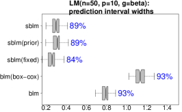
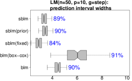
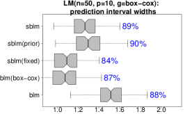
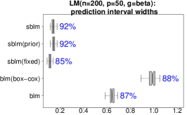
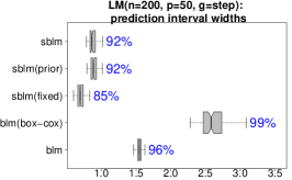
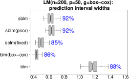
Figure 1: 90% prediction interval widths and empirical coverage (annotated) for out-of-sample prediction with semiparametric Bayesian linear models across various designs. The proposed semiparametric models provide narrow intervals that achieve approximately the correct nominal coverage, with dramatic gains over competing methods for more complex transformations.

Next, we evaluate inference for the regression coefficients $\theta$ using variable selection. Although the scale of $\theta$ depends on the transformation—and thus differs among competing methods—the determination of whether each $\theta_{j}\neq 0$ is more comparable. Here, we select variables if the 95% highest posterior density interval for $\theta_{j}$ excludes zero. The true positive and negative rates are averaged across 100 simulations and presented in Table 1. The transformation is critical: for the beta and step designs, the proposed sblm methods offer a massive increase in the power to detect true effects without incurring more false discoveries. Remarkably, both sblm and sblm(prior) are highly robust to the true transformation and improve rapidly with the sample size, even as $p$ grows. By comparison, blm and blm(box-cox) are excessively conservative in their interval estimates for the regression coefficients and perform well only when the true transformation belongs to the Box-Cox family.

$(n,p)$	design	blm	blm(box-cox)	sblm(fixed)	sblm(prior)	sblm
$(50,10)$	beta	$0.17\quad 0.96$	$0.13\quad 0.96$	$0.85\quad 0.94$	$0.73\quad 0.99$	$0.76\quad 0.98$
	step	$0.58\quad 0.97$	$0.59\quad 0.96$	$0.85\quad 0.94$	$0.74\quad 0.99$	$0.76\quad 0.98$
	box-cox	$0.66\quad 0.94$	$0.90\quad 0.96$	$0.84\quad 0.95$	$0.74\quad 0.99$	$0.76\quad 0.98$
$(200,50)$	beta	$0.18\quad 0.92$	$0.13\quad 0.92$	$1.00\quad 0.95$	$0.99\quad 0.99$	$0.99\quad 0.99$
	step	$0.73\quad 0.99$	$0.25\quad 1.00$	$1.00\quad 0.96$	$0.99\quad 0.99$	$0.99\quad 0.99$
	box-cox	$0.60\quad 0.91$	$1.00\quad 0.96$	$1.00\quad 0.96$	$0.99\quad 0.99$	$0.99\quad 0.99$

Table 1: True positive rates and true negative rates for variable selection across simulation designs for the transformed linear model. When the transformation is more complex, the proposed semiparametric Bayesian linear models deliver a massive increase in power to detect true effects.

We highlight the ability of the sblm and sblm(prior) to infer the various transformations on $\mathcal{Y}=[0,1]$, $\mathcal{Y}=\mathbb{R}^{+}$, and $\mathcal{Y}=\mathbb{R}$. Figure 2 presents 95% pointwise credible intervals for $g$ under these models and blm(box-cox) for a single simulated dataset from each design. The transformations are rescaled such that the posterior means and the true transformations are centered at zero with unit scale, and thus are comparable. Most notably, sblm and sblm(prior) are virtually indistinguishable and successfully concentrate around each true transformation as $n$ grows. By comparison, blm(box-cox) is insufficiently flexible and substantially underestimates the uncertainty about $g$.

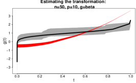
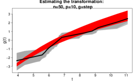
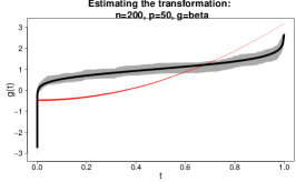
Figure 2: 95% credible intervals for the transformation $g$ using sblm (dark gray), sblm(prior) (light gray), and blm(box-cox) (red) compared to the truth (black). Both of the proposed semiparametric models capture all variety of shapes and concentrate around the truth as $n$ grows.

Remarkably, using the prior distribution for $\hat{p}(\theta\mid\mathcal{D}_{n})$ in (8) and Algorithm 1 (sblm(prior)) performs nearly identically to the data-driven Laplace approximation (sblm) for prediction of $y^{test}$, selection of coefficients $\theta_{j}\neq 0$, and estimation of the transformation $g$. This suggests that our approach, including the approximation strategy from Section 2.2, is robust to the choice of $\hat{p}(\theta\mid\mathcal{D}_{n})$. Clearly, the ability to substitute $p(\theta)$ is highly beneficial, as it is always available and requires no additional computations or tuning.

We briefly mention computing performance. Applying Algorithm 3 as described in Section 2.3, the joint Monte Carlo sampler for $(\theta,g,\tilde{y}(X^{test}))$ requires about 3.5 seconds per 1000 samples for the larger $n=200$, $p=50$ design (using R on a MacBook Pro, 2.8 GHz Intel Core i7). Because these are Monte Carlo (not MCMC) algorithms, no convergence diagnostics, burn-in periods, or inefficiency factors are needed.

3.2 Simulation study for semiparametric Bayesian quantile regression

We modify the simulation design from Section 3.1 to evaluate the proposed semiparametric approach for quantile regression. First, the latent data are generated from $z_{i}=x_{i}^{\mathrm{\scriptscriptstyle T}}\theta_{true}(1+\epsilon_{i})$ with $\epsilon_{i}\sim N(0,1)$, which introduces heteroskedasticity. Heteroskedasticity is a common motivation for quantile regression, since it often leads to different conclusions compared to mean regression. Second, the inverse transformation is simply the identity. Thus, the data-generating process does not implicitly favor the transformed regression model (1)–(3).

We implement the proposed semiparametric Bayesian quantile regression from Section 2.4 with similar variations for inferring $g$ as in Section 3.1. To specify $\hat{p}(\theta\mid\mathcal{D}_{n})$ in (8) and Algorithm 1, we consider both a Laplace approximation using classical quantile regression with bootstrap-based covariance estimate from the R package quantreg (sbqr) and the prior $p(\theta)$ (sbqr(prior)). We also consider the simplification with the transformation fixed at $\hat{g}$ in (6) (sbqr(fixed)). For comparisons, we include Bayesian quantile regression (bqr) without the transformation, which otherwise uses the same sampling steps as in Section 2.4, and frequentist quantile regression (qr) using default settings in quantreg. The Bayesian models use the same $g$-prior with $\mu_{\theta}=0$ and $\Sigma_{\theta}=n\sigma^{2}(X^{\mathrm{\scriptscriptstyle T}}X)^{-1}$. The models are estimated for quantiles $\tau\in\{0.05,0.25,0.50\}$; performance is comparable for large quantiles ($1-\tau$) and the results for $\tau=0.05$ and $\tau=0.10$ are similar. Quantile estimates on the testing data $X^{test}$ are computed using $X^{test}\hat{\theta}$ for qr and bqr and the posterior mean of $g^{-1}(X^{test}\theta)$ for the semiparametric methods.

We evaluate the quantile estimates by computing the proportion of testing data points that are below the estimated $\tau$th quantile (Figure 3). For a well-calibrated quantile estimate, this quantity should be close to $\tau$. Although all methods are well-calibrated for the median $(\tau=0.5)$, the existing frequentist (qr) and Bayesian (bqr) estimates become poorly calibrated as $\tau$ decreases (or increases; not shown). By comparison, the proposed semiparametric methods maintain calibration across all values of $\tau$, especially for the fully Bayesian implementations. Again, we see little difference between the data-driven approximation (sbqr) and the prior approximation (sbqr(prior)) central to (8), which highlights the robustness of Algorithm 1.

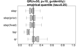
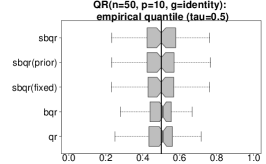
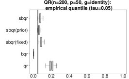
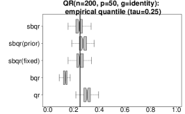
Figure 3: Proportion of testing data below the estimated $\tau$th quantile (vertical line at $\tau$) across 100 simulations. Each method is well-calibrated for the median $(\tau=0.5)$, but the proposed semiparametric estimators are significantly more accurate when $\tau$ is small (or large; not shown).

We emphasize the value of the transformation for improving Bayesian model adequacy. Specifically, we compute continuous ranked probability scores for the posterior predictive draws $\tilde{y}(X^{test})$ from each Bayesian model, and average those across all simulations (Table 2). These scores provide a comprehensive assessment of the out-of-sample posterior predictive distributions. Compared to the standard Bayesian quantile regression model (bqr), the proposed semiparametric modification offers massive improvements in predictive distributional accuracy. In particular, bqr is highly inaccurate for smaller $\tau$, while the sbqr methods are robust across $\tau$. Thus, the semiparametric approach alleviates concerns about the inadequacy of an ALD model and produces more accurate quantile estimates.

Quantile	bqr	sbqr(fixed)	sbqr(prior)	sbqr
$\tau=0.05$	7.55	0.50	0.49	0.50
$\tau=0.25$	1.07	0.41	0.41	0.41
$\tau=0.50$	0.66	0.40	0.40	0.40

Table 2: Continuous ranked probability scores on testing data for Bayesian quantile regression with $n=50,p=10$; results are similar for $n=200,p=50$. The proposed semiparametric Bayesian quantile models offer massive improvements in predictive distributional accuracy.

These important conclusions are confirmed visually by examining posterior predictive diagnostics for a single simulated dataset (Figure 4). We compute the empirical cumulative distribution function for the observed data and for each posterior predictive draw under the Bayesian quantile regression model for each $\tau\in\{0.05,0.25,0.5\}$. Traditional Bayesian quantile regression based on the ALD is clearly inadequate as a data-generating process for all values of $\tau$. By comparison, the proposed semiparametric alternative sbqr (and sbqr(prior); not shown) completely corrects these inadequacies to deliver a model that both infers the target quantiles accurately (Figure 3) and is globally faithful to the observed data (Table 2 and Figure 4).

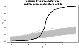
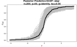
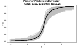
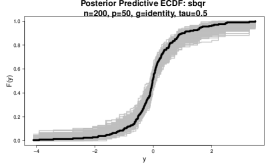
Figure 4: Posterior predictive diagnostics for Bayesian quantile regression based on the empirical cumulative distribution function for each $\tau\in\{0.05,0.25,0.5\}$. The posterior predictive draws (gray lines) are faithful to the observed data (black lines) for the proposed approach (bottom), while traditional Bayesian quantile regression (top) is highly inadequate.

3.3 Semiparametric Gaussian processes for Lidar data

We apply the semiparametric Bayesian Gaussian process model to the Lidar data from Ruppert et al., (2003). These data are a canonical example of a nonlinear and heteroskestastic curve-fitting problem (Figure 5). Instead of augmenting a Gaussian process model with a variance model—which requires additional model specification, positivity constraints, and more demanding computations—we simply apply the proposed semiparametric Bayesian Gaussian process (sbgp) approach from Section 2.5. The latent Gaussian process $f_{\theta}\sim\mathcal{GP}(m_{\theta},K_{\theta})$ features an unknown constant for the mean function $m_{\theta}$ and an isotropic Matérn covariance function $K_{\theta}$ with unknown variance, range, and smoothness parameters; these unknowns constitute $\theta$. Computations of the Gaussian process point estimates, predictions, and covariances are done using the GpGp package in R (Katzfuss and Guinness,, 2021).

First, we assess the sbgp fit to the full dataset ($n=221$). Figure 5 (left) presents the fitted curve and 90% pointwise prediction intervals. The sbgp model is capable of smoothly capturing the trend and the heteroskedasticity in the data—which is not explicitly modeled. More thorough posterior predictive diagnostics (Figure 5, right) confirm the adequacy of the model. Specifically, we compute the empirical cumulative distribution on the data and on each simulated predictive dataset, in both cases restricted to smaller ($x<500$) and larger ($x>500$) covariate values. Despite the notable differences in the distributions, the proposed sbgp is faithful to the data.

For comparison, we include an approximate version that fixes the transformation at $\hat{g}$ in (9) (sbgp(fixed)), and consider more standard Gaussian process models that omit the transformation (gp) or apply an unknown Box-Cox transformation (gp(box-cox)) using the same prior and sampler for $\lambda$ as in Section 3.1. Figure 5 shows that sbgp(fixed) naturally produces narrower prediction intervals, but more importantly, that gp(box-cox) is unable to capture the heteroskedasticity in the data. Thus, unlike the proposed nonparametric Bayesian transformation, the parametric Box-Cox transformation is inadequate for this key distributional feature.

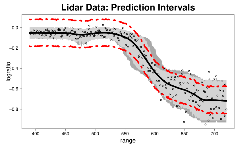
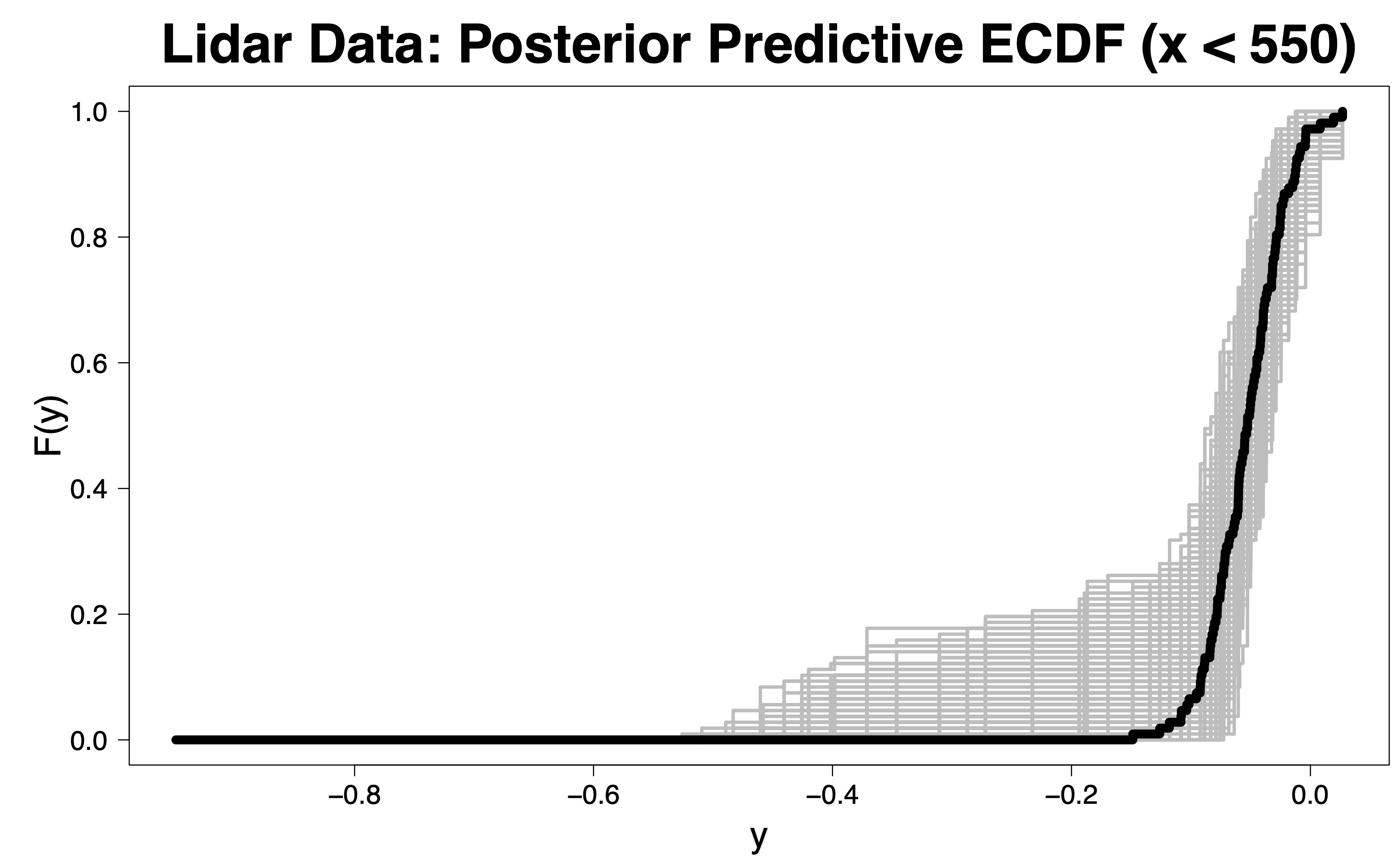
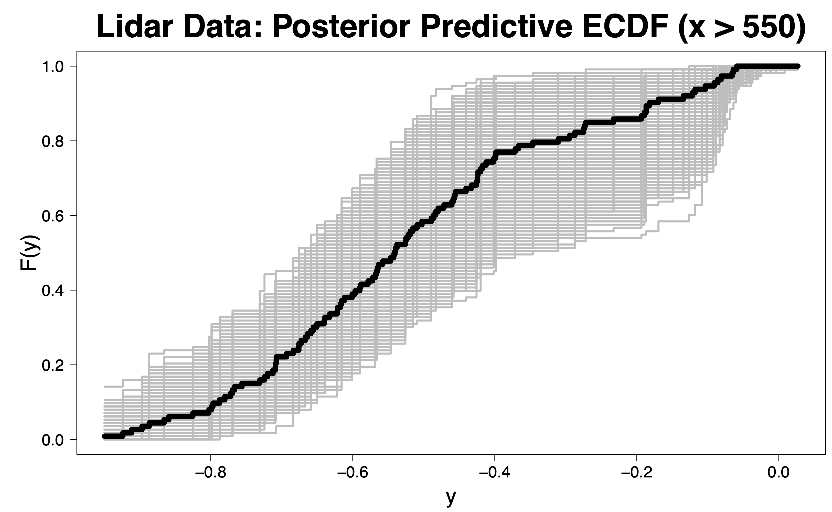
Figure 5: Left: 90% prediction intervals and median (black line) for the Lidar data. The proposed semiparametric Gaussian process model (dark gray) and approximate version (light gray) capture the heteroskedasticity in the data, while the Box-Cox version (dashed red) does not. Right: Posterior predictive diagnostics based on the marginal empirical cumulative distribution function restricted version for smaller (top) and larger (bottom) $x$ values. The posterior predictive draws (gray lines) from sbgp are faithful to the observed data (black lines).

We proceed with more formal evaluations based on 100 random training/testing splits of the data (80% training). Table 3 presents the average interval widths and empirical coverage for 95%, 90%, and 80% out-of-sample prediction intervals. Remarkably, sbgp delivers the exactly correct nominal coverage, often with narrower intervals than the competing gp and gp(box-cox) models. The intervals from the approximate version are narrower and typically close to nominal coverage. The proposed methods are both calibrated and sharp. This is confirmed using out-of-sample ranked probability scores (not shown), which show statistically significant improvements for sbgp(fixed) and sbgp relative to the Gaussian process competitors.

Nominal coverage	gp	gp(box-cox)	sbgp(fixed)	sbgp
95%	0.311 (92%)	0.313 (92%)	0.276 (93%)	0.329 (95%)
90%	0.261 (90%)	0.263 (90%)	0.223 (89%)	0.258 (90%)
80%	0.204 (86%)	0.205 (86%)	0.171 (80%)	0.197 (82%)

Table 3: Average interval width and empirical coverage (parenthetical) for prediction intervals for Lidar data across 100 random training/testing splits. The proposed approaches are well-calibrated (correct coverage) and sharper (narrower intervals) than competing methods.

Finally, we modified the approximate approach from Section 2.5 to include posterior sampling of $f_{\hat{\theta}}$, which accounts for the uncertainty in the regression function (but not the hyperparameters $\theta$). The results were visually indistinguishable from Figure 5, but the computing cost increased substantially: for the full dataset, sbgp required only about 4 seconds per 1000 Monte Carlo samples, while the augmented posterior sampler needed about 111 seconds. These discrepancies increase with $n$. In aggregate, our results suggest that sbgp successfully combines the efficiency of point optimization with the uncertainty quantification from the Bayesian nonparametric model for $g$ to deliver fast, calibrated, and sharp posterior predictive inference.

4 Theory

An important advantage of our modeling and algorithmic framework is that it enables direct asymptotic analysis. We consider generic models for $P_{X}$ and $P_{Y}$ within model (1)–(2) and show that our joint posterior for $(g,\theta)$ under Algorithm 3 is consistent under conditions on $P_{Y}$, $P_{X}$, and $P_{Z\mid\theta,X}$. Importantly, these results verify the asymptotic validity of (i) the surrogate likelihood, (ii) the approximation (8), and (iii) the location-scale robustness adjustment (Section 2.2).

Let $\mathcal{M}(\mathcal{Y})$ denote the space of monotone increasing functions mapping $\mathcal{Y}$ to $\mathbb{R}$ and let $\mathcal{T}$ be the topology of pointwise convergence. Let $F_{X,0}$ and $F_{Y,0}$ denote the true distribution functions of $X$ and $Y$, respectively. Finally, let $\tilde{g}$ be the restriction of $g$ to $\tilde{\mathcal{Y}}=\{y\in\mathcal{Y}:0<F_{Y,0}(y)<1\}$ and $\tilde{g}_{0}$ defined similarly for the true transformation $g_{0}$.

First, we establish posterior consistency for $p(\tilde{g}\mid\mathcal{D}_{n})$ at $\tilde{g}_{0}$.

Theorem 2.

Suppose that the true data-generating process $P_{g_{0},\theta_{0}}$ is identified by the parameters $g_{0}\in(\mathcal{M}(\mathcal{Y}),\mathcal{T})$ and $\theta_{0}\in\mathbb{R}^{d}$ under model (1)–(2). Under the assumptions

1. $F_{Z\mid\theta,X}(t)$ is continuous in $X$, $t$, and in $\theta$ for an open neighborhood of $\theta_{0}$ invariant to $(t,X)$;

2. the posterior approximation $\hat{p}(\theta\mid\mathcal{D}_{n})$ is (strongly) consistent at $\theta_{0}$; and

3. the marginal models $F_{X\mid\mathcal{D}_{n}},F_{Y\mid\mathcal{D}_{n}}$ are (strongly) consistent at $F_{X,0},F_{Y,0}$,

then the posterior distribution $p(\tilde{g}\mid\mathcal{D}_{n})$ is (strongly) consistent at $\tilde{g}_{0}$ under (i) $\mathcal{T}$ and (ii) the $L_{\infty}$-topology on any bounded subset of $\tilde{\mathcal{Y}}$.

Importantly, this posterior $p(\tilde{g}\mid\mathcal{D}_{n})$ refers to the one targeted by Algorithm 3, which uses (i) the surrogate likelihood and (ii) the approximation $\hat{p}(\theta\mid\mathcal{D}_{n})$ in (8). The examples from Section 2 satisfy the conditions on $F_{Z\mid\theta,X}$ (2.1), while the Bayesian bootstrap models for $P_{X}$ and $P_{Y}$ are (weakly) consistent for the margins (2.3). The requirement (2.2) admits many choices of $\hat{p}(\theta\mid\mathcal{D}_{n})$. Perhaps the simplest option is a point mass at some consistent estimator of $\theta_{0}$, such as using rank-based estimators (Horowitz,, 2012; see the supplementary material).

Corollary 1.

Let $\hat{p}(\theta\mid\mathcal{D}_{n})=\delta_{\tilde{\theta}}$, where $\tilde{\theta}\overset{p}{\to}\theta_{0}$ is a consistent point estimator. Under the conditions of Theorem 2, $p(\tilde{g}\mid\mathcal{D}_{n})$ is weakly consistent at $\tilde{g}_{0}$ under $\mathcal{T}$.

To strengthen Theorem 2, we consider special cases of the support $\mathcal{Y}$. The restriction to $\tilde{\mathcal{Y}}$ ensures that $g$ is finite, but the limiting cases are well-defined: we may set $g(t)=-\infty$ for any $t$ such that $F_{Y,0}(t)=0$ and similarly $g(t)=\infty$ whenever $F_{Y,0}(t)=1$. No such consideration is needed when $\mathcal{Y}$ is unbounded.

Corollary 2.

Suppose $\mathcal{Y}$ is unbounded. Under the conditions of Theorem 2, $p(g\mid\mathcal{D}_{n})$ is (strongly) consistent at $g_{0}$ under (i) $\mathcal{T}$ and (ii) the $L_{\infty}$-topology on any bounded subset of $\tilde{\mathcal{Y}}$.

When $\mathcal{Y}$ is compact, we can strengthen this result to uniform posterior consistency of $p(g\mid\mathcal{D}_{n})$ with no restrictions. Uniform posterior consistency ensures that the posterior converges to the true parameter at the same rate in all regions of the domain. This is particularly important when the shape of the true transformation is not known a priori.

Corollary 3.

Suppose $\mathcal{Y}$ is compact. Under the conditions of Theorem 2, $p(g\mid\mathcal{D}_{n})$ is weakly consistent at $g_{0}$ under the $L_{\infty}$-topology.

Building upon Theorem 2, we establish joint posterior consistency of $(g,\theta)$ by showing consistency of the conditional posterior $p(\theta\mid\mathcal{D}_{n},g)$ with fixed transformation $g$. For robustness, we provide sufficient conditions for strong posterior consistency of $p(\theta\mid\mathcal{D}_{n},g)$ without assuming the correctness of the model for $\theta$. Instead, we target the parameter that minimizes Kullback–Leibler (KL) divergence from an arbitrary data-generating process to the assumed model.

Theorem 3.

Let $P_{0}$ be the true data-generating process and $P_{g,\theta}$ the data-generating model induced by (1)–(2) with $g\in(\mathcal{M}(\mathcal{Y}),\mathcal{T})$ and $\theta\in\Theta\subseteq\mathbb{R}^{d}$. Let $\Pi_{\theta}$ be the prior on $\theta$ and $p(Y\mid g,\theta,X)$ the likelihood of $\theta$ at $(X,Y)$ and conditional on $g$. Under the assumptions

1. there exists a unique $\theta^{*}(g)\in\mbox{int}(\Theta)$ such that $\theta^{*}(g)=\arg\min_{\theta\in\Theta}KL(P_{0},P_{g,\theta})$;

2. $|\mathbb{E}_{P_{0}}\log p(Y\mid g,\theta,X)|<\infty$ for all $\theta\in\Theta$;

3. the mapping $\theta\mapsto\log p(Y\mid g,\theta,X)$ is concave almost surely $[P_{0}]$; and

4. $\Pi_{\theta}(\mathcal{U})>0$ for any open neighborhood $\mathcal{U}$ that contains $\theta^{*}(g)$,

then $p(\theta\mid\mathcal{D}_{n},g)$ is strongly consistent at $\theta^{*}(g)$ under the Euclidean topology for every fixed $g$.

The target posterior $p(\theta\mid\mathcal{D}_{n},g)=p(\theta\mid\{x_{i},g(y_{i})\}_{i=1}^{n})$ is equivalently the posterior distribution under (2) using transformed data $\{x_{i},g(y_{i})\}_{i=1}^{n}$ with known $g$. Thus, some form of posterior consistency is unsurprising for many continuous regression models (2). Instead, Theorem 3 is valuable because (i) it establishes strong consistency for $\theta^{*}(g)$ under model misspecification and (ii) it may be combined with the previous (strong) consistency results for $p(g\mid\mathcal{D}_{n})$ to establish the joint posterior consistency of $(g,\theta)$.

Corollary 4.

Suppose that the true data-generating process $P_{g_{0},\theta_{0}}$ is uniquely identified by the parameters $g_{0}\in(\mathcal{M}(\mathcal{Y}),\mathcal{T})$ and $\theta_{0}\in\mathbb{R}^{d}$ under model (1)–(2). If the assumptions (2.1)–(2.3), (3.1)–(3.4) hold for all $g$, and if $\theta^{*}(g)$ is continuous at $g_{0}$, then the joint posterior distribution $p(\tilde{g},\theta\mid\mathcal{D}_{n})$ is (strongly) consistent at $(\tilde{g}_{0},\theta_{0})$.

The conditions (2.2)–(2.3) refer to our model for $g$ under (6) and Algorithm 3, while (2.1) and (3.1)–(3.4) are regularity requirements on the model (2) and the prior for $\theta$. Additional restrictions such as those in Corollaries 1–3 may be applied similarly as before.

Finally, we assess the proposed robustness strategy to misspecification of $F_{Z\mid\mathcal{D}_{n}}$. When $F_{Z\mid\mathcal{D}_{n}}$ is misspecified in location or scale, accurate estimation of $g$ is impossible (Lemma 1). We consider the case in which $p(g\mid\mathcal{D}_{n})$ converges to the wrong transformation, and specifically one that differs by a shift and scaling. The proposed strategy (Section 2.2) is to replace $P_{Z\mid X,\theta}$ with $\mu+\sigma P_{Z\mid X,\theta}$ in (2), but only for the conditional posterior $p(\theta\mid\mathcal{D}_{n},g)$ in (4).

Theorem 4.

Let $P_{0}$ be the true data-generating process and $P_{g,\theta}$ the data-generating model induced by (1)–(2) with $g\in(\mathcal{M}(\mathcal{Y}),\mathcal{T})$ and $\theta\in\Theta\subseteq\mathbb{R}^{d}$. Suppose that $(g_{0},\theta_{0})=\arg\min_{g,\theta}\text{KL}(P_{0},P_{g,\theta})$ exists and is unique. Let $\mu+\sigma P_{Z\mid\theta,X}$ be identifiable with respect to $(\mu,\sigma,\theta)$ and assume prior independence $\Pi_{\mu,\sigma,\theta}=\Pi_{\mu,\sigma}\times\Pi_{\theta}$. Suppose that $p(\tilde{g}\mid\mathcal{D}_{n})$ is (strongly) consistent at $\mu_{0}+\sigma_{0}\tilde{g}_{0}$, where $\mu_{0}$ and $\sigma_{0}\neq 0$ are constants and $(\mu_{0},\sigma_{0})\in\text{supp}(\Pi_{\mu,\sigma})$. Under the key assumption

1. there exists a neighborhood $\mathcal{G}$ around $\mu_{0}+\sigma_{0}g_{0}$ under the topology $\mathcal{T}$ such that for any $g_{n}\to g$ in $\mathcal{G}$, $\sup_{\mu\in\mathbb{R},\sigma\in\mathbb{R}^{+},\theta\in\Theta}|KL(P_{0},P_{(g_{n}-\mu)/\sigma,\theta})-KL(P_{0},P_{(g-\mu)/\sigma,\theta})|\to 0$,

and if assumptions (3.1)–(3.4) hold for all $g$, then the joint posterior distribution $p(\tilde{g},\theta\mid\mathcal{D}_{n})$ is (strongly) consistent at $(\mu_{0}+\sigma_{0}\tilde{g}_{0},\theta_{0})$.

This theorem provides robustness guarantees for the model (1)–(2) under double misspecifications of both $\theta$ and $g$, and in particular ensures marginal (strong) consistency of $p(\theta\mid\mathcal{D}_{n})$ at $\theta_{0}$. Specifically, $\theta$ may be misspecified in the sense that the true parameter is not contained in the parameter set $\Theta$, and $g$ may be misspecified as a location-scale shift around $g_{0}$, where $g_{0}$ is a fixed monotonic transformation. Notably, this result does not require $g_{0}$ and $\theta_{0}$ to be the true parameters, but instead establishes posterior consistency for any pair of the transformation $g_{0}$ and the KL-minimizer $\theta_{0}$, as long as the conditions are satisfied. The main condition, (4.1) appears complex but is a common requirement in the asymptotic analysis of misspecified Bayesian semiparametric models. It is a variant of similar conditions related to posterior convergence under perturbations around “least-favorable submodels” of the true model (Bickel and Kleijn,, 2012).

5 Discussion

We introduced a Bayesian approach for semiparametric regression analysis. Our strategy featured a transformation layer (1) atop a continuous regression model (2) to enhance modeling flexibility, especially for irregular marginal distributions and various data domains. Most uniquely, the proposed sampling algorithm (Algorithm 3) delivered efficient Monte Carlo (not MCMC) inference with easy implementations for popular regression models such as linear regression, quantile regression, and Gaussian processes. Empirical results demonstrated exceptional prediction, selection, and estimation capabilities for Bayesian semiparametric linear models; substantially more accurate quantile estimates and model adequacy for Bayesian quantile regression; and superior predictive accuracy for Gaussian processes. Finally, our asymptotic analysis established joint posterior consistency under general conditions, including multiple model misspecifications.

The primary concerns with Algorithm 3 are (i) the use of the surrogate likelihood in place of (7) and (ii) the need for an approximation $\hat{p}(\theta\mid\mathcal{D}_{n})$ to infer $g$ via (8). We have attempted to address these concerns using both empirical and theoretical analysis. The empirical results are highly encouraging: the Monte Carlo samplers are efficient and simple for a variety of semiparametric Bayesian models and the posterior predictive distributions are calibrated and sharp for many challenging simulated and real datasets. These results are robust to the choice of the approximation, including simply the prior $\hat{p}(\theta\mid\mathcal{D}_{n})=p(\theta)$. Further, we introduced an importance sampling adjustment to provide posterior inference under the correct likelihood. Yet this adjustment does not appear to make any difference in practice, even for $n=50$, which is reassuring for direct and unadjusted application of Algorithm 3. Finally, the theoretical analysis establishes the asymptotic validity of the posterior targeted by Algorithm 3, even under multiple model misspecifications. This remains true for a broad class of (consistent) marginal models for $P_{Y}$ and $P_{X}$, which allows customization for settings in which the Bayesian bootstrap is not ideal.

References

- Atkinson et al., (2021) Atkinson, A. C., Riani, M., and Corbellini, A. (2021). The Box-Cox Transformation: Review and Extensions. Statistical Science, 36(2):239–255.
- Bean et al., (2016) Bean, A., Xu, X., and MacEachern, S. (2016). Transformations and Bayesian density estimation. Electronic Journal of Statistics, 10(2):3355–3373.
- Bickel and Kleijn, (2012) Bickel, P. J. and Kleijn, B. J. K. (2012). The semiparametric Bernstein–von Mises theorem. The Annals of Statistics, 40(1):206–237.
- Box and Cox, (1964) Box, G. E. P. and Cox, D. R. (1964). An analysis of transformations. Journal of the Royal Statistical Society: Series B (Methodological), 26(2):211–243.
- Breiman and Friedman, (1985) Breiman, L. and Friedman, J. H. (1985). Estimating optimal transformations for multiple regression and correlation. Journal of the American statistical Association, 80(391):580–598.
- Carroll and Ruppert, (1988) Carroll, R. J. and Ruppert, D. (1988). Transformation and weighting in regression, volume 30. CRC Press.
- Chen et al., (2002) Chen, K., Jin, Z., and Ying, Z. (2002). Semiparametric analysis of transformation models with censored data. Biometrika, 89(3):659–668.
- Cheng et al., (1995) Cheng, S. C., Wei, L. J., and Ying, Z. (1995). Analysis of transformation models with censored data. Biometrika, 82(4):835–845.
- De Oliveira et al., (1997) De Oliveira, V., Kedem, B., and Short, D. A. (1997). Bayesian prediction of transformed Gaussian random fields. Journal of the American Statistical Association, 92(440):1422–1433.
- Durante, (2019) Durante, D. (2019). Conjugate Bayes for probit regression via unified skew-normal distributions. Biometrika, 106(4):765–779.
- Fan et al., (2016) Fan, J., Xue, L., and Zou, H. (2016). Multitask quantile regression under the transnormal model. Journal of the American Statistical Association, 111(516):1726–1735.
- Fasano and Durante, (2020) Fasano, A. and Durante, D. (2020). A class of conjugate priors for multinomial probit models which includes the multivariate normal one. arXiv preprint arXiv:2007.06944.
- Feldman and Kowal, (2022) Feldman, J. and Kowal, D. R. (2022). Bayesian data synthesis and the utility-risk trade-off for mixed epidemiological data. Annals of Applied Statistics, 16(4):2577–2602.
- Fritsch and Carlson, (1980) Fritsch, F. N. and Carlson, R. E. (1980). Monotone piecewise cubic interpolation. SIAM Journal on Numerical Analysis, 17(2):238–246.
- Ghosal and Van der Vaart, (2017) Ghosal, S. and Van der Vaart, A. (2017). Fundamentals of nonparametric Bayesian inference, volume 44. Cambridge University Press.
- Grazian and Liseo, (2017) Grazian, C. and Liseo, B. (2017). Approximate Bayesian inference in semiparametric copula models. Bayesian Analysis, 12(4):991–1016.
- Hoff, (2007) Hoff, P. D. (2007). Extending the rank likelihood for semiparametric copula estimation. The Annals of Applied Statistics, 1(1):265–283.
- Horowitz, (2012) Horowitz, J. L. (2012). Semiparametric Methods in Econometrics, volume 131. Springer Science & Business Media.
- Huggins et al., (2018) Huggins, J. H., Campbell, T., Kasprzak, M., and Broderick, T. (2018). Practical bounds on the error of Bayesian posterior approximations: A nonasymptotic approach. arXiv preprint arXiv:1809.09505.
- Joe, (2005) Joe, H. (2005). Asymptotic efficiency of the two-stage estimation method for copula-based models. Journal of multivariate Analysis, 94(2):401–419.
- Katzfuss and Guinness, (2021) Katzfuss, M. and Guinness, J. (2021). A general framework for Vecchia approximations of Gaussian processes. Statistical Science, 36(1):124–141.
- Klein and Smith, (2019) Klein, N. and Smith, M. S. (2019). Implicit copulas from Bayesian regularized regression smoothers. Bayesian Analysis, 14(4):1143–1171.
- Kowal and Canale, (2020) Kowal, D. R. and Canale, A. (2020). Simultaneous Transformation and Rounding (STAR) Models for Integer-Valued Data. Electronic Journal of Statistics, 14(1):1744–1772.
- Kowal and Wu, (2022) Kowal, D. R. and Wu, B. (2022). Semiparametric discrete data regression with Monte Carlo inference and prediction. arXiv preprint arXiv:2110.12316.
- Kozumi and Kobayashi, (2011) Kozumi, H. and Kobayashi, G. (2011). Gibbs sampling methods for Bayesian quantile regression. Journal of statistical computation and simulation, 81(11):1565–1578.
- Kruskal, (1965) Kruskal, J. B. (1965). Analysis of factorial experiments by estimating monotone transformations of the data. Journal of the Royal Statistical Society: Series B (Methodological), 27(2):251–263.
- Lázaro-Gredilla, (2012) Lázaro-Gredilla, M. (2012). Bayesian warped Gaussian processes. In Advances in Neural Information Processing Systems, pages 1619–1627.
- Lin and Joseph, (2020) Lin, L.-H. and Joseph, V. R. (2020). Transformation and additivity in Gaussian processes. Technometrics, 62(4):525–535.
- Lin and Jeon, (2003) Lin, Y. and Jeon, Y. (2003). Discriminant analysis through a semiparametric model. Biometrika, 90(2):379–392.
- Liu et al., (2009) Liu, H., Lafferty, J., and Wasserman, L. (2009). The nonparanormal: Semiparametric estimation of high dimensional undirected graphs. Journal of Machine Learning Research, 10(10):2295–2328.
- Mallick and Gelfand, (1994) Mallick, B. K. and Gelfand, A. E. (1994). Generalized linear models with unknown link functions. Biometrika, 81(2):237–245.
- Mallick and Walker, (2003) Mallick, B. K. and Walker, S. (2003). A Bayesian semiparametric transformation model incorporating frailties. Journal of Statistical Planning and Inference, 112(1-2):159–174.
- Maroñas et al., (2021) Maroñas, J., Hamelijnck, O., Knoblauch, J., and Damoulas, T. (2021). Transforming Gaussian processes with normalizing flows. In International Conference on Artificial Intelligence and Statistics, pages 1081–1089. PMLR.
- Mulgrave and Ghosal, (2020) Mulgrave, J. J. and Ghosal, S. (2020). Bayesian Inference in Nonparanormal Graphical Models. Bayesian Analysis, 15(2):449–475.
- Neal, (2003) Neal, R. M. (2003). Slice sampling. Annals of Statistics, pages 705–741.
- Pericchi, (1981) Pericchi, L. R. (1981). A Bayesian approach to transformations to normality. Biometrika, 68(1):35–43.
- Pettitt, (1982) Pettitt, A. N. (1982). Inference for the linear model using a likelihood based on ranks. Journal of the Royal Statistical Society: Series B (Methodological), 44(2):234–243.
- Ramsay, (1988) Ramsay, J. O. (1988). Monotone regression splines in action. Statistical science, 3(4):425–441.
- Rios and Tobar, (2018) Rios, G. and Tobar, F. (2018). Learning non-Gaussian Time Series using the Box-Cox Gaussian Process. Proceedings of the International Joint Conference on Neural Networks, 2018-July.
- Rios and Tobar, (2019) Rios, G. and Tobar, F. (2019). Compositionally-warped Gaussian processes. Neural Networks, 118:235–246.
- Rubin, (1981) Rubin, D. B. (1981). The Bayesian bootstrap. The Annals of Statistics, pages 130–134.
- Ruppert et al., (2003) Ruppert, D., Wand, M. P., and Carroll, R. J. (2003). Semiparametric regression. Number 12. Cambridge University Press.
- Smith and Klein, (2021) Smith, M. S. and Klein, N. (2021). Bayesian inference for regression copulas. Journal of Business & Economic Statistics, 39(3):712–728.
- Snelson et al., (2003) Snelson, E., Ghahramani, Z., and Rasmussen, C. (2003). Warped gaussian processes. Advances in neural information processing systems, 16.
- Song and Lu, (2012) Song, X.-Y. and Lu, Z.-H. (2012). Semiparametric transformation models with Bayesian P-splines. Statistics and Computing, 22(5):1085–1098.
- Tang et al., (2018) Tang, N., Wu, Y., and Chen, D. (2018). Semiparametric Bayesian analysis of transformation linear mixed models. Journal of Multivariate Analysis, 166:225–240.
- Tibshirani, (1988) Tibshirani, R. (1988). Estimating transformations for regression via additivity and variance stabilization. Journal of the American Statistical Association, 83(402):394–405.
- Wang and Dunson, (2011) Wang, L. and Dunson, D. B. (2011). Semiparametric Bayes’ proportional odds models for current status data with underreporting. Biometrics, 67(3):1111–1118.
- Wu et al., (2019) Wu, Y., Chen, D., and Tang, N. (2019). Semiparametric Bayesian analysis of transformation spatial mixed models for large datasets. Statistics and Its Interface, 12(4):549–560.
- Yu and Moyeed, (2001) Yu, K. and Moyeed, R. A. (2001). Bayesian quantile regression. Statistics & Probability Letters, 54(4):437–447.
- Zellner, (1986) Zellner, A. (1986). On assessing prior distributions and Bayesian regression analysis with g-prior distributions. Bayesian inference and decision techniques.