Constraining supermassive primordial black holes with magnetically induced gravitational waves

Abstract

Primordial black holes (PBHs) can answer a plethora of cosmic conundra, among which the origin of the cosmic magnetic fields. In particular, supermassive PBHs with masses $M_{\mathrm{PBH}}>10^{10}M_{\odot}$ and furnished with a plasma-disk moving around them can generate through the Biermann battery mechanism a seed primordial magnetic field which can later be amplified so as to provide the magnetic field threading the intergalactic medium. In this work, we derive the gravitational wave (GW) signal induced by the magnetic anisotropic stress of such a population of magnetised PBHs. Interestingly enough, by using GW constraints from Big Bang Nucleosynthesis (BBN) and an effective model for the galactic/turbulent dynamo amplification of the magnetic field, we set a conservative upper bound constraint on the abundances of supermassive PBHs at formation time, $\Omega_{\mathrm{PBH,f}}$ as a function of the their masses, namely that $\Omega_{\mathrm{PBH,f}}\leq 2.5\times 10^{-10}\left(\frac{M}{10^{10}M_{\odot}}\right)^{45/22}$. Remarkably, these constraints are comparable, and, in some mass ranges, even tighter compared to the constraints on $\Omega_{\mathrm{PBH,f}}$ from large-scale structure (LSS) probes; hence promoting the portal of magnetically induced GWs as a new probe to explore the enigmatic nature of supermassive PBHs.

I Introduction

The origin of the primordial magnetic fields (MFs) threading the intergalactic medium constitutes one of the longstanding issues in cosmology. These cosmic MFs can play a crucial role in the processes of particle acceleration through the intergalactic medium Bagchi et al. (2002), of the propagation of cosmic rays Strong et al. (2007) while at the same time, they can affect significantly the Universe’s thermal state between inflation and recombination Grasso and Rubinstein (1996); Barrow et al. (1997); Subramanian (2006).

Among their generation mechanisms, there have been proposed processes related to phase transitions in the early Universe Turner and Widrow (1988); Quashnock et al. (1989), primordial scalar Ichiki et al. (2006); Naoz and Narayan (2013); Flitter et al. (2023) and vector perturbations Banerjee and Jedamzik (2003); Durrer (2007) as well as astrophysical ones seeding battery-induced MFs Biermann (1950). In particular, in the last years there has been witnessed a rekindled interest connecting the origin of primordial MFs with primordial black holes (PBHs) Safarzadeh (2018); Araya et al. (2021); Papanikolaou and Gourgouliatos (2023). As it was recently shown in Papanikolaou and Gourgouliatos (2023) supermassive PBHs furnished with a disk can generate through the Biermann-battery mechanism the seed for the primordial MFs of $10^{-18}\mathrm{G}$ observed in intergalactic scales Dermer et al. (2011).

Interestingly enough, PBHs, firstly introduced in ’70s can address a swathe of modern cosmological enigmas. In particular, they can naturally account for a fraction or even the totality of dark matter Chapline (1975); Clesse and García-Bellido (2018) explaining as well LSS formation through Poisson fluctuations Meszaros (1975); Afshordi et al. (2003); Carr and Rees (1984) and providing the seeds of the supermassive black holes residing in galactic centres Bean and Magueijo (2002); De Luca et al. (2023); Li et al. (2023); Su et al. (2023). At the same time, they are associated with numerous GW signals related to PBH merging events Nakamura et al. (1997); Eroshenko (2018); Raidal et al. (2017), Hawking radiation Anantua et al. (2009); Dong et al. (2016); Ireland et al. (2023) and enhanced cosmological Saito and Yokoyama (2009); Bugaev and Klimai (2010); Kohri and Terada (2018) adiabatic and isocurvature perturbations Papanikolaou et al. (2021); Domènech et al. (2021, 2022); Papanikolaou (2022). See here for recent reviews Sasaki et al. (2018); Domènech (2021).

In this work, we derive the GW signal induced by the magnetic anisortropic stress of a population of magnetised supermassive PBHs. Accounting as well for GW constraints from BBN we are able to set tight constraints on the abundances of supermassive PBHs promoting in this way the magnetically induced GWs (MIGWs) as a novel portal shedding light to the field of PBH physics.

II The seed primordial magnetic field à la Biermann

PBH accretion disks have been recently proposed as a candidate to generate the seed primordial MFs threading the intergalactic medium Safarzadeh (2018); Araya et al. (2021); Papanikolaou and Gourgouliatos (2023). In particular, the ab initio generation of a seed MF requires the relative motion between negative and positive charges, conditions which can be achieved in a highly turbulent medium such as the primordial plasma between BBN and recombination  Kurskov and Ozernoi (1974a, b); Trivedi et al. (2018); Roper Pol (2021). Under such conditions, a Biermann battery mechanism operates whenever the energy density and temperature gradients are not parallel to each other Blandford et al. (1983). Consequently, one is inevitably met with the following magnetic field induction equation

$$\partial_{t}{\bf B}=\nabla\left({\bf u}\times{\bf B}\right)-\frac{ck_{B}}{e}\frac{\nabla\rho\times\nabla T}{\rho}\,,$$ (1)

where the second term in the right hand side is the Biermann battery one.

In order to derive the Biermann battery induced MF one should assume an equation of state (EoS) for the vortex-like moving plasma around the black hole. Doing so, we assume a locally isothermal disk around the PBH D’Angelo and Lubow (2010), where the density and the pressure are related through the following relation:

$$p(R,\phi,z)=\rho(R,\phi,z)c_{s}^{2}(R)\,,$$ (2)

where $(R,\phi,z)$ are the cylindrical coordinates. This EoS can describe quite well a gas that radiates internal energy gained by shocks Lubow et al. (1999), here produced by the turbulent motion of the primordial plasma expected after BBN and before recombination era Kurskov and Ozernoi (1974a, b); Trivedi et al. (2018); Roper Pol (2021).

At the end, accounting for the random spatial distribution of PBHs and considering monochromatic PBH mass distributions, after a long but straightforward calculation [For more details see Papanikolaou and Gourgouliatos (2023)] one can extract the MF power spectrum, which can be recast as 

$$\begin{split}P_{B}(k,t_{\mathrm{s}})&\simeq 4\times 10^{-86}q^{2}\ell^{4}_{R}\Omega^{2}_{\mathrm{PBH,f}}\\ &\times\left(\frac{M}{10^{10}M_{\odot}}\right)^{2}\left(\frac{k}{\mathrm{Mpc}^{-1}}\right)^{3}\left[\mathrm{G^{2}Mpc^{3}}\right],\end{split}$$ (3)

where $\ell_{R}=R_{\mathrm{d}}/R_{\mathrm{ISCO}}$ is the ratio of the radius of the disk, $R_{\mathrm{d}}$ over the radius of the innermost stable circular orbit, $R_{\mathrm{ISCO}}$ and $q=H_{\mathrm{d}}/R_{\mathrm{ISCO}}$ is the ratio of the thickness of the disk $H_{\mathrm{d}}$ over $R_{\mathrm{ISCO}}$ which is less than $1$ since Eq. (5) was extracted within the thin-disk limit where one is usually met with sub-Eddington accretion Shakura and Sunyaev (1973); Pringle and Rees (1972); Lynden-Bell and Pringle (1974). It is important to notice that the above mentioned MF power spectrum was extracted at saturation time $t_{\mathrm{s}}$, namely at the end of the linear growth phase of the MF, [See the Biermann-battery term in Eq. (1)] and for scales larger than the PBH mean separation scale, so as not to enter the non-linear regime. This imposes a UV-cutoff scale $k_{\mathrm{UV}}$ which can be recast straightforwardly as $k_{\mathrm{UV}}=10^{19}M_{\odot}\Omega^{1/3}_{\mathrm{PBH,f}}\mathrm{Mpc}^{-1}/M$ Papanikolaou and Gourgouliatos (2023).

One can derive as well the mean MF amplitude which is defined as

$$\langle|{\boldsymbol{B}}_{\boldsymbol{k}}|\rangle\equiv\mathchoice{{\hbox{$\displaystyle\sqrt{\frac{k^{3}P_{B}(k)}{2\pi^{2}}\,}$}\lower 0.4pt\hbox{\vrule height=14.4711pt,depth=-11.57693pt}}}{{\hbox{$\textstyle\sqrt{\frac{k^{3}P_{B}(k)}{2\pi^{2}}\,}$}\lower 0.4pt\hbox{\vrule height=10.15553pt,depth=-8.12447pt}}}{{\hbox{$\scriptstyle\sqrt{\frac{k^{3}P_{B}(k)}{2\pi^{2}}\,}$}\lower 0.4pt\hbox{\vrule height=7.84859pt,depth=-6.2789pt}}}{{\hbox{$\scriptscriptstyle\sqrt{\frac{k^{3}P_{B}(k)}{2\pi^{2}}\,}$}\lower 0.4pt\hbox{\vrule height=7.84859pt,depth=-6.2789pt}}}.$$ (4)

Accounting therefore for cosmic expansion, i.e. $B\sim a^{-2}$, and plugging now Eq. (3) into Eq. (4) one gets the mean MF amplitude in intergalactic scales, i.e. $k\sim 100\mathrm{Mpc}^{-1}$, which reads as

$$B\sim 10^{-30}q\left(\frac{\ell_{\mathrm{R}}}{10^{6}}\right)^{2}\left(\frac{M_{\mathrm{PBH}}}{10^{14}M_{\odot}}\right)^{5/2}\quad(\mathrm{G}).$$ (5)

Interestingly enough, by taking typical values of $q\sim 0.001-1$ and varying the parameter $\ell_{R}$ with the range $\ell_{R}\in[10^{2},10^{11}]$ depending on the accretion rate McKinney et al. (2012), one can produce for PBH masses $M\in[10^{10},10^{16}]M_{\odot}$  a seed primordial MF of the order $10^{-32}-10^{-29}\mathrm{G}$, which is actually the minimum seed MF amplitude needed to give rise, through dynamo/turbulent amplification, to the present-day average magnetic field of order $10^{-18}\mathrm{G}$ in intergalactic scales Vachaspati (2021).

III The magnetic field anisotropic stress

Let us now extract the magnetic anisotropic stress induced by such a MF power spectrum. In particular, regarding the stress-energy tensor associated to a magnetic field ${\boldsymbol{B}}$, this can be recast in the following covariant form:

$$T^{(B)}_{ij}\equiv\frac{1}{4\pi}\left[\frac{B^{2}g_{ij}}{2}-B_{i}B_{j}\right].$$ (6)

From Eq. (6) one can define an associated anisotropic stress as follows

$$\Pi_{ij}({\boldsymbol{k}})\equiv\left(P^{l}_{i}P^{m}_{j}-\frac{P_{ij}P^{lm}}{2}\right)T_{lm}({\boldsymbol{k}}),$$ (7)

where $P_{ij}$ is a projection matrix defined as $P_{ij}\equiv\delta_{ij}-\hat{{\boldsymbol{k}}}_{i}\hat{{\boldsymbol{k}}}_{j}$ and $\hat{{\boldsymbol{k}}}={\boldsymbol{k}}/k$. From Eq. (7) one can define the equal-time 2-point correlator of the magnetic anisotropic stress as:

$$\langle\Pi_{ij}({\boldsymbol{k}},\eta)\Pi_{ij}({\boldsymbol{q}},\eta)\rangle\equiv\Pi_{B}(k,\eta)\delta({\boldsymbol{k}},{\boldsymbol{q}}),$$ (8)

where $\Pi_{B}({\boldsymbol{k}},\eta)$ is the power spectrum of the magnetic anisotropic stress related with the magnetic field power spectrum $P_{B}(k,\eta)$ as follows Caprini and Durrer (2006):

$$\Pi_{B}(k,\eta)=\int\mathrm{d}^{3}{\boldsymbol{q}}P_{B}(q,\eta)P_{B}(|{\boldsymbol{q}}-{\boldsymbol{k}}|,\eta)(1+\gamma^{2})(1+\beta^{2}),$$ (9)

where $\gamma=\hat{{\boldsymbol{k}}}\cdot\hat{{\boldsymbol{q}}}$ and $\beta=\hat{{\boldsymbol{k}}}\cdot\widehat{{\boldsymbol{k}}-{\boldsymbol{q}}}$.

Introducing now the auxiliary variables $v$ and $u$ such as that $u=|{\boldsymbol{q}}-{\boldsymbol{k}}|/k$ and $v=q/k$ after some algebraic manipulations one can recast the above equation in the following form:

$$\begin{split}&\Pi_{B}(k,\eta)=2\pi k^{3}\int_{0}^{\mathrm{\frac{k_{\mathrm{UV}}}{k}}}\mathrm{d}v\int_{|1-v|}^{1+v}\mathrm{d}uP_{B}(kv,\eta)P_{B}(ku,\eta)uv\\ &\times\left[1+\frac{(1+v^{2}-u^{2})^{2}}{4v^{2}}\right]\left[1+\left(1-\frac{1+v^{2}-u^{2}}{2v}\right)^{2}\right].\end{split}$$ (10)

At the end, plugging Eq. (3) in Eq. (9) one gets that

$$\begin{split}\Pi_{B}(k,\eta)&\simeq 10^{-170}q^{4}\ell^{8}_{R}\Omega^{4}_{\mathrm{PBH,f}}10^{-174}\left(\frac{k}{\mathrm{Mpc}^{-1}}\right)^{9}\\ &\times\left(\frac{M}{10^{10}M_{\odot}}\right)^{4}f\left(\frac{k_{\mathrm{UV}}}{k}\right)\mathrm{G^{4}Mpc^{3}},\end{split}$$ (11)

where $f(\frac{k_{\mathrm{UV}}}{k})$ is the double integral over $u$ and $v$ which is defined as follows:

$$\begin{split}f\left(\frac{k_{\mathrm{UV}}}{k}\right)\equiv&\int_{0}^{\frac{k_{\mathrm{UV}}}{k}}\mathrm{d}v\int_{|1-v|}^{1+v}\mathrm{d}uu^{4}v^{4}\left[1+\frac{(1+v^{2}-u^{2})^{2}}{4v^{2}}\right]\\ &\times\left[1+\left(1-\frac{1+v^{2}-u^{2}}{2v}\right)^{2}\right].\end{split}$$ (12)

After performing the integration one can show that

$$\begin{split}&f\left(y\equiv\frac{k_{\mathrm{UV}}}{k}\right)=\frac{32}{45}y^{9}-\frac{131y^{8}}{60}+\frac{293y^{7}}{98}-\frac{3323y^{6}}{1680}\\ &+\frac{27229y^{5}}{50400}-\frac{2y^{4}}{105}+\frac{26y^{3}}{3465}-\frac{2y^{2}}{1155}+\frac{8y}{15015}-\frac{19711}{6306300}.\end{split}$$ (13)

In the region away from the UV-cutoff scale $k_{\mathrm{UV}}$, namely when $k_{\mathrm{UV}}/k\gg 1$, one obtains that $f\left(y\equiv\frac{k_{\mathrm{UV}}}{k}\right)\simeq(32/45)(k_{\mathrm{UV}}/k)^{9}$.

IV Magnetically induced gravitational waves

Having extracted above the power spectrum of the magnetic anisotropic stress we study here the dynamics of the tensor perturbations $h_{\boldsymbol{k}}$ induced by such an anisotropic stress. In particular, the equation of motion for $h_{\boldsymbol{k}}$ can be recast as Caprini and Durrer (2006):

$$h_{\boldsymbol{k}}^{s,\prime\prime}+2\mathcal{H}h_{\boldsymbol{k}}^{s,\prime}+k^{2}h^{s}_{\boldsymbol{k}}=\frac{8\pi G}{a^{2}}\mathchoice{{\hbox{$\displaystyle\sqrt{\Pi_{B}(k,\eta)\,}$}\lower 0.4pt\hbox{\vrule height=7.5pt,depth=-6.00003pt}}}{{\hbox{$\textstyle\sqrt{\Pi_{B}(k,\eta)\,}$}\lower 0.4pt\hbox{\vrule height=7.5pt,depth=-6.00003pt}}}{{\hbox{$\scriptstyle\sqrt{\Pi_{B}(k,\eta)\,}$}\lower 0.4pt\hbox{\vrule height=5.25pt,depth=-4.20003pt}}}{{\hbox{$\scriptscriptstyle\sqrt{\Pi_{B}(k,\eta)\,}$}\lower 0.4pt\hbox{\vrule height=3.75pt,depth=-3.00002pt}}},$$ (14)

where $s=(+),(\times)$ stands for the two polarisation states of the tensor modes in general relativity.

An analytic solution to Eq. (14) can be obtained by using the Green’s function formalism. Namely, one gets that

$$h^{s}_{\boldsymbol{k}}(\eta)=8\pi G\int^{\eta}_{\eta_{0}}\mathrm{d}\bar{\eta}\,g_{\boldsymbol{k}}(\eta,\bar{\eta})\frac{\mathchoice{{\hbox{$\displaystyle\sqrt{\Pi_{B}(k,\bar{\eta})\,}$}\lower 0.4pt\hbox{\vrule height=7.5pt,depth=-6.00003pt}}}{{\hbox{$\textstyle\sqrt{\Pi_{B}(k,\bar{\eta})\,}$}\lower 0.4pt\hbox{\vrule height=7.5pt,depth=-6.00003pt}}}{{\hbox{$\scriptstyle\sqrt{\Pi_{B}(k,\bar{\eta})\,}$}\lower 0.4pt\hbox{\vrule height=5.67776pt,depth=-4.54224pt}}}{{\hbox{$\scriptscriptstyle\sqrt{\Pi_{B}(k,\bar{\eta})\,}$}\lower 0.4pt\hbox{\vrule height=5.67776pt,depth=-4.54224pt}}}}{a^{2}(\bar{\eta})},$$ (15)

where $g_{\boldsymbol{k}}(\eta,\bar{\eta})$ is the Green’s function being the solution of the homogeneous equation (14) without the source term [See Caprini and Durrer (2006) for more details]. For the case of an RD era, $w=1/3$, when PBHs typically form, one gets that

$$kg^{\mathrm{RD}}_{\boldsymbol{k}}(\eta,\bar{\eta})=\sin(x-\bar{x}).$$ (16)

One then can define the GW spectral abundance as $\Omega_{\mathrm{GW}}(\eta,k)\equiv\frac{1}{\rho_{\mathrm{c}}}\frac{\mathrm{d}\rho_{\mathrm{GW}}}{\mathrm{d}\ln k}$, where $\rho_{\mathrm{c}}=3H^{2}/(8\pi G)$ is the critical energy density, and show that it can be recast as Maggiore (2000); Kohri and Terada (2018)

$$\Omega_{\mathrm{GW}}(\eta,k)=\frac{1}{24}\left[\frac{k}{\mathcal{H}(\eta)}\right]^{2}\overline{\mathcal{P}}_{h}(\eta,k),$$ (17)

where $\mathcal{H}$ is the conformal Hubble parameter and $\mathcal{P}_{h}(\eta,k),$ is the tensor power spectrum defined as

$$\mathcal{P}_{h}(\eta,k)\equiv\frac{k^{3}|h_{\boldsymbol{k}}|^{2}}{2\pi^{2}}.$$ (18)

The bar denotes averaging over the sub-horizon oscillations of the tensor field, which is done in order to extract the envelope of the GW spectrum at those scales.

Combining therefore Eq. (11), Eq. (15), Eq. (16), Eq. (18) and Eq. (17), one obtains that the GW spectral abundance will read as

$$\begin{split}\Omega_{\mathrm{GW}}(\eta,k)&=10^{-70}I^{2}(x)\left(\frac{k}{\mathrm{Mpc}^{-1}}\right)\\ &\times\left(\frac{10^{10}M_{\odot}}{M}\right)^{4}\ell^{8}_{R}\Omega^{7}_{\mathrm{PBH,f}},\end{split}$$ (19)

where $x=k\eta$ and $I(x)$ is defined as

$$I(x)\equiv\int_{x_{\mathrm{dyn}}}^{x}\mathrm{d}\bar{x}\frac{\sin(x-\bar{x})}{\bar{x}^{2}}\left[1-\frac{x^{2}_{\mathrm{dyn}}}{\bar{x}^{2}}\right]^{2},$$ (20)

where $\eta_{\mathrm{dyn}}$ stands for the conformal disk dynamical time and $x_{\mathrm{dyn}}=k\eta_{\mathrm{dyn}}\simeq 1$ since the disk establishes very quickly its hydrostatic equilibrium on the vertical axis soon after the PBH formation time, which is standardly considered as the time when the typical size of the collapsing overdensity region $r\sim 1/k$ crosses the cosmological horizon, i.e. when $k=aH$. Thus, one has that $\eta_{\mathrm{dyn}}\simeq\eta_{\mathrm{f}}$ and that $x_{\mathrm{dyn}}=k\eta_{\mathrm{dyn}}\simeq k\eta_{\mathrm{f}}=k/(a_{\mathrm{f}}H_{\mathrm{f}})=1$.

V Non-amplified magnetically induced gravitational waves

In what follows, we will account for the contribution of the magnetic anisotropic stress during the time interval where the Biermann battery mechanism operates within its linear growth regime up to $t=t_{\mathrm{s}}$, hence underestimating the GW signal and considering that the tensor modes propagate as free GWs up to our present day soon after the end of the era of the linear growth of ${\boldsymbol{B}}$ at $t=t_{\mathrm{s}}$.

Thus, for $x=x_{\mathrm{s}}=\mathchoice{{\hbox{$\displaystyle\sqrt{2\,}$}\lower 0.4pt\hbox{\vrule height=6.44444pt,depth=-5.15558pt}}}{{\hbox{$\textstyle\sqrt{2\,}$}\lower 0.4pt\hbox{\vrule height=6.44444pt,depth=-5.15558pt}}}{{\hbox{$\scriptstyle\sqrt{2\,}$}\lower 0.4pt\hbox{\vrule height=4.51111pt,depth=-3.6089pt}}}{{\hbox{$\scriptscriptstyle\sqrt{2\,}$}\lower 0.4pt\hbox{\vrule height=3.22221pt,depth=-2.57779pt}}}x_{\mathrm{dyn}}$ Papanikolaou and Gourgouliatos (2023) one can check numerically that $I^{2}(x_{\mathrm{s}})\simeq 10^{-5}$. At the end, accounting for the fact that $a^{2}H^{2}\propto a^{-2}$ in the RD era one gets that

$$\begin{split}\Omega_{\mathrm{GW}}(\eta_{\mathrm{s}},k)&=10^{-75}\left(\frac{k}{\mathrm{Mpc}^{-1}}\right)\\ &\times\left(\frac{10^{10}M_{\odot}}{M}\right)^{4}\ell^{8}_{R}\Omega^{7}_{\mathrm{PBH,f}}.\end{split}$$ (21)

One then can compute the GW spectral abundance $\Omega_{\mathrm{GW}}(\eta,k)$ at our present epoch as follows:

$$\begin{split}\Omega_{\mathrm{GW}}(\eta_{0},k)&=\frac{\rho_{\mathrm{GW}}(\eta_{0},k)}{\rho_{\mathrm{c}}(\eta_{0})}=\frac{\rho_{\mathrm{GW}}(\eta_{\mathrm{s}},k)}{\rho_{\mathrm{c}}(\eta_{\mathrm{s}})}\left(\frac{a_{\mathrm{s}}}{a_{\mathrm{0}}}\right)^{4}\frac{\rho_{\mathrm{c}}(\eta_{\mathrm{s}})}{\rho_{\mathrm{c}}(\eta_{0})}\\ &=c_{g}\Omega^{(0)}_{\mathrm{r}}\Omega_{\mathrm{GW}}(\eta_{\mathrm{s}},k),\end{split}$$ (22)

where $c_{g}=\frac{\rho_{\mathrm{r,s}}a^{4}_{\mathrm{s}}}{\rho_{\mathrm{r,0}}a^{4}_{0}}\simeq 0.4$ Espinosa et al. (2018), $\Omega^{(0)}_{\mathrm{r}}\sim 10^{-5}$ and we have taken into account as well that $\Omega_{\mathrm{GW}}\sim a^{-4}$. The index $0$ refers to the present time. Finally, $\Omega_{\mathrm{GW}}(\eta_{0},k)$ will be recast as

$$\begin{split}\Omega_{\mathrm{GW}}(\eta_{0},k)&\simeq 3\times 10^{-81}\left(\frac{k}{\mathrm{Mpc}^{-1}}\right)\left(\frac{10^{10}M_{\odot}}{M}\right)^{4}q^{4}\ell^{8}_{R}\Omega^{7}_{\mathrm{PBH,f}}.\end{split}$$ (23)

Regarding now the GW frequency this will be given by $f=k/(2\pi a_{0})$ where we conventionally take $a_{0}=1$. Thus, since $k\leq k_{\mathrm{UV}}$, one can extract an upper bound constraint on the GW frequency, namely that

$$\begin{split}f&\leq f_{\mathrm{max}}=\frac{k_{\mathrm{UV}}}{2\pi}=10^{5}\frac{M_{\odot}}{M}\Omega^{1/3}_{\mathrm{PBH,f}}\\ &\leq 3\times 10^{-7}\left(\frac{10^{10}M_{\odot}}{M}\right)^{5/6}\leq 3\times 10^{-7}\quad\mathrm{(Hz)},\end{split}$$ (24)

since $M>10^{10}M_{\odot}$ and $\Omega_{\mathrm{PBH,f}}<2.6\times 10^{-5}\mathchoice{{\hbox{$\displaystyle\sqrt{\frac{M}{10^{10}M_{\odot}}\,}$}\lower 0.4pt\hbox{\vrule height=12.00775pt,depth=-9.60625pt}}}{{\hbox{$\textstyle\sqrt{\frac{M}{10^{10}M_{\odot}}\,}$}\lower 0.4pt\hbox{\vrule height=8.4333pt,depth=-6.74667pt}}}{{\hbox{$\scriptstyle\sqrt{\frac{M}{10^{10}M_{\odot}}\,}$}\lower 0.4pt\hbox{\vrule height=6.4222pt,depth=-5.13779pt}}}{{\hbox{$\scriptscriptstyle\sqrt{\frac{M}{10^{10}M_{\odot}}\,}$}\lower 0.4pt\hbox{\vrule height=6.4222pt,depth=-5.13779pt}}}$ so as not to overproduce PBHs at matter-radiation equality. Therefore the relevant MIGW signal is far away from the frequency bands of the Laser Space Inferometer Antenna (LISA) Caprini et al. (2016); Karnesis et al. (2022), Einstein Telscope (ET) Maggiore et al. (2020) and Big Bang Observer (BBO) Harry et al. (2006) GW detectors. Potentially, it can be well within the Square Kilometer Array (SKA) Janssen et al. (2015), the NANOGrav Agazie et al. (2023) and the PTA Reardon et al. (2023); Antoniadis et al. (2023) frequency detection band. However, for smaller mass PBHs furnished with a disk, which however will not be able to seed primordial MFs Papanikolaou and Gourgouliatos (2023) the GW frequency will increase and can be well within LISA, ET and BBO frequency detection bands.

Apart from the GW frequency, one should check as well the GW amplitude (23). In particular, considering that $k\leq k_{\mathrm{UV}}$, $\ell_{R}\leq 10^{11}$ and accounting for Eq. (23) as well as for the fact that for $M>10^{10}M_{\odot}$, $\Omega_{\mathrm{PBH,f}}<2.6\times 10^{-5}\left(\frac{M}{10^{10}M_{\odot}}\right)^{1/2}$, one gets an upper bound on $\Omega_{\mathrm{GW}}(\eta_{0})$ which reads as

$$\Omega_{\mathrm{GW}}(\eta_{0})<7\times 10^{-18}\left(\frac{10^{10}M_{\odot}}{M}\right)^{4/3}\leq 7\times 10^{-18},$$ (25)

and which is slightly below the lowest GW sensitivity of current and future GW detectors being of the order of $10^{-15}$. Consequently, these magnetically induced GWs can hardly be detected by current/future GW detectors.

VI Amplified magnetically induced gravitational waves

However, up to now, we have not accounted for the turbulent and galactic dynamo or the magnetorotational instability Velikhov (1959); Chandrasekhar (1960); Balbus and Hawley (1991) amplification which will play a significant role after matter-radiation equality during the non-linear growth of the matter perturbations. These amplification mechanisms can significantly enhance the MF amplitude and at the end the GW signal potentially putting it within the sensitivity bands of current/future GW detectors. To account therefore for these effects we introduce the amplification factor $\alpha(k)$ as the ratio between the amplified MF over the non-amplified MF, i.e.

$$\alpha(k)=\frac{B^{\mathrm{amplified}}(k)}{B^{\mathrm{non-amplified}}(k)}.$$ (26)

To extract the function $\alpha(k)$ over the different scales $k$ at hand one should run high-cost numerical MHD simulations so as to account for the various turbulent/galactic dynamo and instability processes, something which is beyond the scope of this work. Thus, in order to make below quantitative predictions for the GW signal, we will assume an effective power-law toy model for $\alpha(k)$ which can be recast as

$$\alpha(k)=\alpha(k_{*})\left(\frac{k}{k_{*}}\right)^{n_{B}},$$ (27)

where $k_{*}$ is a pivot scale and $n_{B}$ is the amplification spectral index which should be greater or equal to zero since in small scales one expects to have a greater MF amplification . In what follows, we will consider as our pivot scale the characteristic intergalactic scale $k_{*}=100\mathrm{Mpc}^{-1}$ where we know from observations that $B\sim 10^{-18}\mathrm{G}$ Dermer et al. (2011) and thus $\alpha(k_{*})$ will read as

$$\begin{split}&\alpha(k_{*}=100\mathrm{Mpc}^{-1})=\frac{10^{-18}}{10^{-30}\mathrm{G}q\left(\frac{\ell_{\mathrm{R}}}{10^{6}}\right)^{2}\left(\frac{M_{\mathrm{PBH}}}{10^{14}M_{\odot}}\right)^{5/2}}\\ &=\frac{10^{22}}{q}\left(\frac{10^{6}}{\ell_{R}}\right)^{2}\left(\frac{10^{10}M_{\odot}}{M}\right)^{5/2},\end{split}$$ (28)

where we have used Eq. (5) for the non-amplified MF amplitude on intergalactic scales.

This amplification effect will give an extra $a^{2}(k)$ factor at the level of the MF power spectrum $P_{B}(k)$ since $P_{B}(k)\propto B^{2}_{k}$. At the end, one is met with a rough overall $a^{4}(k)$ amplification factor at the level of the GW signal since $\Omega_{\mathrm{GW}}\propto\int\int P^{2}_{B}$ as we can see from Eq. (15), Eq. (10) and Eq. (17). Thus, multiplying Eq. (23) with $\alpha^{4}(k)$ one gets that

$$\begin{split}\Omega_{\mathrm{GW}}(k,\eta_{0})&\simeq 3\times 10^{55-8n_{B}}\left(\frac{k}{\mathrm{Mpc}^{-1}}\right)^{4n_{B}+1}\\ &\times\left(\frac{10^{10}M_{\odot}}{M}\right)^{14}\Omega^{7}_{\mathrm{PBH,f}}\end{split}$$ (29)

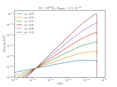
Figure 1: The gravitational-wave spectrum induced by a population of magnetised PBHs with mass $M=10^{10}M_{\odot}$ and initial PBH abundance at formation time $\Omega_{\mathrm{PBH,f}}=4\times 10^{-12}$ for different values of the amplification spectral index $n_{B}$.

VII Constraints on supermassive primordial black holes

Let us see now how one can constrain the abundances of such supermassive PBHs using the aforementioned GW portal. Interestingly enough, one can set an upper bound on $\Omega_{\mathrm{PBH,f}}$ by accounting for the contribution of the GWs to the effective number of extra neutrino species $\Delta N_{\mathrm{eff}}$. In particular, one can translate the upper bound from Planck for the amplitude of GWs today, namely that $\Omega_{\mathrm{GW}}(\eta_{0})\leq 10^{-6}$ Caprini and Figueroa (2018); Aghanim et al. (2020), to an upper bound on $\Omega_{\mathrm{PBH,f}}$.

As we see from Eq. (29), for $k\geq 100\mathrm{Mpc}^{-1}$ the GW amplitude increases with $n_{B}$. Thus, in order to get a conservative constraint on $\Omega_{\mathrm{PBH,f}}$ we will choose the flat case where $n_{B}=0$. At the end, by using Eq. (29) for $n_{B}=0$ and setting $k=k_{\mathrm{UV}}$, since at $k\sim k_{\mathrm{UV}}$ one gets the maximum GW amplitude [See Fig. 1], we obtain a conservative upper bound constraint on $\Omega_{\mathrm{PBH,f}}$ by just simply requiring that $\Omega_{\mathrm{GW}}(\eta_{0})\leq 10^{-6}$ reading as 

$$\Omega_{\mathrm{PBH,f}}\leq 2.5\times 10^{-10}\left(\frac{M}{10^{10}M_{\odot}}\right)^{45/22}.$$ (30)

Remarkably, this upper bound constraint on $\Omega_{\mathrm{PBH,f}}$ is comparable and in some mass regions tighter compared to constraints on $\Omega_{\mathrm{PBH,f}}$ from LSS probes, which were derived by simply requiring that galaxies should not form too early Carr and Silk (2018); Carr et al. (2021). Interestingly, if one increases the amplification spectral index $n_{B}$ they get tighter constraints on $\Omega_{\mathrm{PBH,f}}$ up to $10^{15}M_{\odot}$. See Fig. 2 for more details. Therefore, the portal of GWs induced by magnetised PBHs is inevitably promoted as a new probe to explore the enigmatic nature of supermassive PBHs.

Here, it is important to highlight however that we did not consider $\mu$ and $y$ distortions of the Cosmic Microwave Background (CMB) affected by PBH formation which put strong constraints on $\Omega_{\mathrm{PBH,f}}$ assuming Gaussian primordial perturbations Kohri et al. (2014); Karam et al. (2023). These strong constraints can in general be evaded assuming non-Gaussian cosmological perturbations Nakama et al. (2016); Kawasaki and Murai (2019); Hooper et al. (2023a), hence we do not consider them in this work.

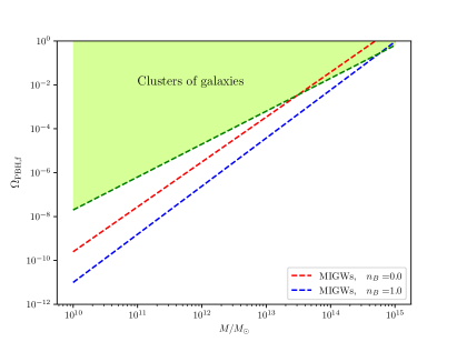
Figure 2: The constraints on the initial PBH abundance at formation time $\Omega_{\mathrm{PBH,f}}$ as a function of the PBH mass $M$ for $n_{B}=0$ (dashed red curve) and $n_{B}=1$ (dashed blue curve). In the green region we show the constraints on $\Omega_{\mathrm{PBH,f}}$ from galaxy clusters Carr and Silk (2018).

VIII Discussion

The origin of cosmic magnetic fields constitutes one of the longstanding issues in cosmology. Among their generation mechanisms the portal of magnetised PBHs seeding battery-induced cosmic MFs seems one of the most promising.

In this work, we have considered a population of supermassive PBHs furnished with a locally isothermal disk which can generate through Biermann-battery a seed primordial MF in the intergalactic scales. In particular, we derived for the first time the GWs induced by the magnetic anisotropic stress of such a population of magnetised PBHs.

Interestingly enough, by accounting for the contribution of the MIGWs to the effective number of extra neutrino species $\Delta N_{\mathrm{eff}}$ and adopting an effective model for the galactic/turbulent dynamo amplification of the magnetic field, we set upper bound constraints on the abundances of supermassive PBHs at formation time, $\Omega_{\mathrm{PBH,f}}$ as a function of the their masses which reads as

$$\Omega_{\mathrm{PBH,f}}\leq 2.5\times 10^{-10}\left(\frac{M}{10^{10}M_{\odot}}\right)^{45/22}.$$ (31)

In particular, as one may see from Fig. 2, these constraints are comparable and in some mass ranges even tighter compared to constraints on $\Omega_{\mathrm{PBH,f}}$ derived from clusters of galaxies. One should account as well for constraints on supermassive PBHs due to dark matter halo accretion after matter-radiation equality as discussed in Serpico et al. (2020), where it was derived a mass-independent upper bound constraint on the contribution of PBHs to dark matter, $f_{\mathrm{PBH}}\equiv\Omega_{\mathrm{PBH}}/\Omega_{\mathrm{DM}}$, of the order of $3\times 10^{-9}$. However, the aforementioned accretion constraint is not so robust for PBH masses larger than $10^{4}M_{\odot}$, as the ones considered here, since one finds super-Eddington accretion at this high mass range.

At this point, it is noteworthy to mention that in the present work we consider thin accretion disks usually exhibiting sub-Eddington accretion Shakura and Sunyaev (1973); Pringle and Rees (1972); Lynden-Bell and Pringle (1974), which in our case operate only during the linear growth of the magnetic field up to few dynamical times Papanikolaou and Gourgouliatos (2023). Note also that the only place in our analysis where one is met with a dependence on the accretion model is the dimensionless parameter $\ell_{R}$ giving us the radial size of the disk, which in general depends on the accretion rate McKinney et al. (2012). Interestingly enough, this parameter cancels out in the final expression Eq. (29) for the GW signal today since one needs to multiply $\alpha^{4}\propto\ell^{-4}_{R}$ [See Eq. (27) and Eq. (28)] with Eq. (23). In order to extract a potentially more stringent accretion constraint on the PBH abundances in the mass region $M_{\mathrm{PBH}}>10^{4}M_{\odot}$ one needs in principle to run dedicated hydro-dynamical simulations in a cosmological setting, going beyond the scope of the current work. Thus, in the absence of numerical simulations for accretion in the very high PBH mass regime Serpico et al. (2020), it can be claimed that the portal of MIGWs can act as a novel alternative probe to constrain the abundances of supermassive PBHs.

This portal of MIGWs can also be used in order to constrain lower mass PBHs furnished with Biermann battery induced MF which however do not generate the necessary seed primordial MF to give rise to a MF amplitude of the order $10^{-18}\mathrm{G}$, threading the intergalactic medium Papanikolaou and Gourgouliatos (2023). Nevertheless, there exist other MF generation mechanisms, like the cosmic battery one Contopoulos and Kazanas (1998); Contopoulos et al. (2006, 2018), able to give a very high MF amplification on intergalactic scales operating on lower black hole masses, i.e. $M<10^{10}M_{\odot}$.

Furthermore, it is important to emphasize here that within this work we assume the standard PBH formation scenario where PBHs form out of the collapse of enhanced cosmological perturbations with a mass of the order of that within the cosmological horizon Musco and Miller (2013) at the time of PBH formation, remaining agnostic on the specific cosmological model giving rise to enhanced cosmological perturbations. In order to access the exact PBH mass distribution, one should choose a particular cosmological model giving rise to PBH formation and account for the critical collapse scaling law for the PBH mass spectrum Niemeyer and Jedamzik (1998); Musco et al. (2009) as well for the effect of primordial non-Gaussianities which are necessary to avoid the $\mu$ and $y$ distortion constraints. These effects lead in principle to extended PBH mass functions. In this work, we assume for simplicity a monochromatic PBH mass distribution. This choice can be sufficiently justified only for sharply peaked primordial curvature power spectra which, in the presence of non-Gaussian cosmological perturbations, lead to nearly monochromatic PBH mass distributions Yoo et al. (2019); Matsubara and Sasaki (2022). Our work however can be easily generalised to account as well for extended PBH mass distributions using the formalism developed in Araya et al. (2021); Papanikolaou and Gourgouliatos (2023).

We should point out as well here that since we use a simplified effective model in order to capture the MF amplification due to galactic/turbulent dynamo and various instability processes we underestimate the GW amplitude and therefore set conservative constraints on $\Omega_{\mathrm{PBH,f}}$. Full MHD numerical simulations are required, however, in order account for the convective term in the MF induction equation and account for the aforementioned MF amplifications effects.

Finally, let us highlight that the formalism developed within this work regarding the derivation of the magnetically induced GWs is quite generic and can be applied to any population of magnetised PBHs Karas and Stuchlik (2023), e.g. PBHs with magnetic charge Maldacena (2021) or Kerr-Newmann PBHs Hooper et al. (2023b), thus promoting the portal of MIGWs to a new GW counterpart associated to PBHs, potentially detectable by current/future GW detectors.