Can the Low Redshift Lyman Alpha Forest Constrain AGN Feedback Models?

Abstract

We investigate the potential of low-redshift Lyman alpha (Ly$\alpha$) forest for constraining active galactic nuclei (AGN) feedback models by analyzing the Illustris and IllustrisTNG simulation at $z=0.1$. These simulations are ideal for studying the impact of AGN feedback on the intergalactic medium (IGM) as they share initial conditions with significant differences in the feedback prescriptions. Both simulations reveal that the IGM is significantly impacted by AGN feedback. Specifically, feedback is stronger in Illustris and results in reducing cool baryon fraction to 23% relative to 39% in IllustrisTNG. However, when comparing various statistics of Ly$\alpha$ forest such as 2D and marginalized distributions of Doppler widths and H i column density, line density, and flux power spectrum with real data, we find that most of these statistics are largely insensitive to the differences in feedback models. This lack of sensitivity arises because of the fundamental degeneracy between the fraction of cool baryons and the H i photoionization rate ($\Gamma_{\rm HI}$) as their product determines the optical depth of the Ly$\alpha$ forest. Since the $\Gamma_{\rm HI}$ cannot be precisely predicted from first principles, it needs to be treated as a nuisance parameter adjusted to match the observed Ly$\alpha$ line density. After adjusting $\Gamma_{\rm HI}$, the distinctions in the considered statistics essentially fade away. Only the Ly$\alpha$ flux power spectrum at small spatial scales exhibits potentially observable differences, although this may be specific to the relatively extreme feedback model employed in Illustris. Without independent constraints on either $\Gamma_{\rm HI}$ or cool baryon fraction, constraining AGN feedback with low-redshift Ly$\alpha$ forest will be very challenging.

1 Introduction

One of the major unsolved problems in galaxy formation is the physical mechanism that quenches star formation in massive galaxies, resulting in the observed dichotomy between blue star-forming and red-and-dead elliptical galaxies. In order to reproduce this, cosmological simulations often include AGN feedback, which extracts energy from central supermassive black holes and drives powerful galactic outflows that suppress star formation in massive galaxies at late times. The mechanisms by which AGN feedback occurs, such as the episodic quasar mode triggered by major merger events (Springel, 2005; Hopkins et al., 2008) or the continuous radio mode (Croton et al., 2006; Sijacki et al., 2007), are not yet fully understood and are a subject of ongoing debate. The multitude of modeling prescriptions used in recent simulations, such as Horizon-AGN (Dubois et al., 2014), EAGLE (Schaye et al., 2015), Illustris (Genel et al., 2014), IllustrisTNG (Weinberger et al., 2017) and SIMBA (Davé et al., 2019), demonstrate the challenges of understanding this process and the importance of constraining it with observations.

In these simulations, AGN feedback drives powerful outflows that suppress star formation in massive galaxies and therefore can alter the physical state of gas in the circumgalactic and intergalactic media (CGM and IGM) surrounding these galaxies. This process, in addition to accretion shocks in the halos of galaxies, creates a bubble of tenuous, warm-hot gas ($T\sim 10^{5-7}$ K, $n_{\rm H}\leq 10^{-4}$ cm^-3) around halos up to several Mpc in scale, known as the warm-hot IGM (WHIM). The amount of matter in the WHIM phase is related to the ‘missing baryon problem’, which refers to the deficit of baryons in the present-day universe compared to the amount synthesized in the Big Bang (e.g. Persic & Salucci, 1992; Fukugita et al., 1998). Approximately 30-40% of the total baryons are currently unaccounted for at $z<1$ (see e.g Lehner et al., 2007; Prochaska et al., 2009; Shull et al., 2012), compared to the precisely determined abundance from the cosmic microwave background at $z\sim 1100$ and big bang nucleosynthesis (Planck Collaboration et al., 2018) . These missing baryons are difficult to detect because the diffuse gas in the WHIM phase is notoriously challenging to observe. While there have been various claims of detection through X-ray emission (Eckert et al., 2015), stacking the feature arising from the Sunyaev-Zeldovich effect (Tanimura et al., 2019; de Graaff et al., 2019), X-ray absorption lines (e.g. O vii and O viii; Nicastro et al., 2018, but see Johnson et al. 2019), and countless Hubble Space Telescope (HST) UV absorption spectroscopy studies modeling both metals (O vi and Ne viii; Tripp et al., 2008; Savage et al., 2014; Werk et al., 2016; Hussain et al., 2017; Burchett et al., 2019) and broad Lyman-$\alpha$ (Ly$\alpha$ hereafter) absorbers (e.g. Savage et al., 2011; Narayanan et al., 2012; Tejos et al., 2016), robust quantitative constraints on the fraction of cosmic baryons in this WHIM phase have proven elusive.

Theoretically, the missing baryons can be tracked in hydrodynamic simulations (e.g Davé et al., 2001; Martizzi et al., 2019; Tuominen et al., 2021), which predict that even in the absence of AGN feedback, accretion shocks in the halos of galaxies resulting from structure formation alone implies that 30-50% of baryons reside in filaments and halos at the nodes of the cosmic web, shock heated to $T\sim 10^{5-7}$ K by $z<1$ (Cen & Ostriker, 1999, 2006; Davé & Tripp, 2001). The total amount of diffuse gas in the WHIM phase is a combination of the contribution from structure formation and the consequences of energetic feedback events (see e.g Tornatore et al., 2010).

At $z>2$, the vast majority of baryons are known to reside primarily in a $\sim 10^{4}$ K, photoionized phase probed by the Ly$\alpha$ forest ($>80\%$; Prochaska et al., 2009), and cosmological simulations suggest that feedback from galaxies has a negligible impact on the IGM at these redshifts (Kollmeier et al., 2006; Viel et al., 2013b; Chabanier et al., 2020). This is also supported by the percent level agreement between the statistical properties of the Ly$\alpha$ forest and simulations which do not include feedback (Viel & Haehnelt, 2006; Lee et al., 2015; Walther et al., 2019). However, whether AGN feedback sufficiently alters the structure of the Ly$\alpha$ forest at later times $z<1$ is a fundamental open question.

To address this question, we compare the results of two state-of-the-art galaxy formation simulations: the original Illustris simulation (Genel et al., 2014) and its successor IllustrisTNG (Weinberger et al., 2017). These simulations are well-suited for comparison because they share the same underlying code, initial conditions, and similar cosmological parameters. The main difference between them is in the implementation of galaxy formation feedback, specifically the persistent radio-mode AGN feedback. Illustris used strong radio-mode thermal feedback, while IllustrisTNG used mild kinetic radio-mode feedback, resulting in significant differences in the distribution of baryons around massive halos and in the intergalactic medium (IGM). In this work, we focus on the Ly$\alpha$ forest at a $z=0.1$ to investigate the impact of AGN feedback on the IGM.

We use high signal-to-noise quasar spectra from the low-redshift IGM survey of Danforth et al. (2016) to generate forward-modeled Ly$\alpha$ forest spectra from Illustris and IllustrisTNG simulations. We fit the Ly$\alpha$ absorption lines in these simulated spectra and the observed data using an automated Voigt profile fitting code. We use the results of it to fix the hydrogen photoionization rate ($\Gamma_{\rm HI}$) in both simulations in order to match the absorption line density ($\rm{\rm dN/dz}$) observed in the data. We show that, fixing $\Gamma_{\rm HI}$ in this way is crucial for the analysis since it removes the degeneracy between the $\rm{\rm dN/dz}$ and $\Gamma_{\rm HI}$. We then examine various statistics, including the line-of-sight flux power spectrum, the joint distribution of line widths ($b$) and neutral hydrogen (H i) column densities ($N_{\rm HI}$), as well as their respective marginalized distributions, and H i column density distribution function to assess the impact of AGN feedback on the IGM. Our results suggest that feedback has a non-negligible effect on the IGM, but the currently available data do not have sufficient signal-to-noise ratio or resolution to clearly detect it.

However, differences in the gas distribution around halos of massive galaxies between Illustris and IllustrisTNG are significant. In a forthcoming follow-up paper (referred to as Paper II, Khaire et al., 2023, under review), the analysis is repeated exclusively around massive halos to investigate the effects of feedback.

The paper is structured as follows. In Section 2, we describe the simulations used in the study, including their differences in the implementation of feedback and the resulting differences in the temperature and density of the gas in the IGM. In Section 3, we outline the procedure for generating synthetic Ly$\alpha$ forest spectra from the simulations, generating forward models, and performing Voigt profile fitting. In Section 4, we discuss the importance and method for tuning the $\Gamma_{\rm HI}$. In Section 5, we examine the IGM in both simulations using various statistics and discuss our results. The implications of our findings are discussed in Section 6, and a summary is provided in Section 7.

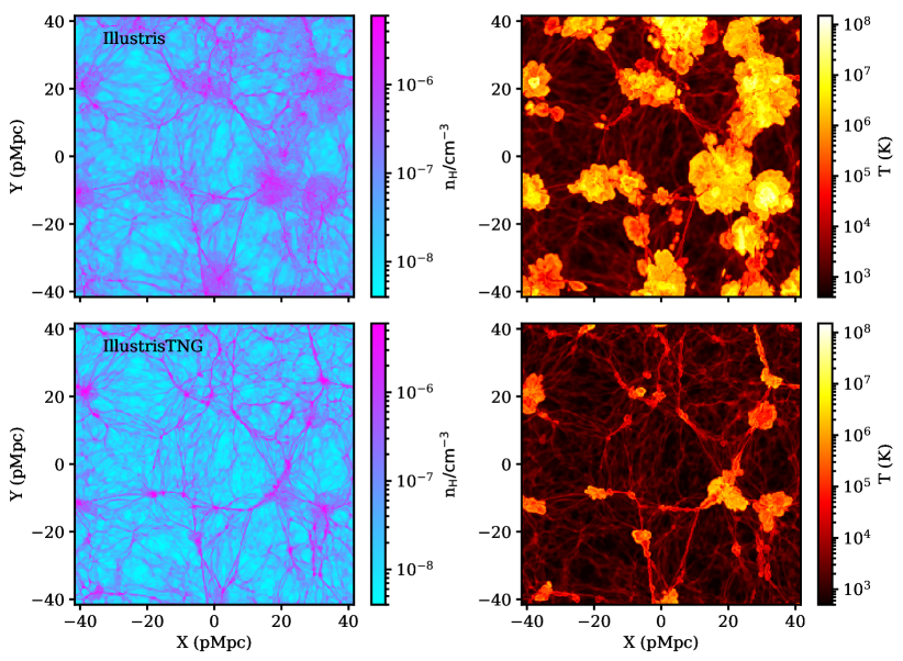
Figure 1: The figure compares the density $n_{\text{H}}$ (left) and temperature $T$ (right) of gas at the same location in Illustris (top) and IllustrisTNG (bottom) simulations at $z=0.1$. Each panel shows a 2D slice (size of $\sim 80$ pMpc) of the simulation with a single cell width of $\sim 60$ ckpc. The distribution of $n_{\text{H}}$ and $T$ is clearly different in the two simulations, particularly around the nodes in the cosmic web where halos reside. This difference is primarily due to the implementation of the radio-mode AGN feedback in both simulations; the explosive feedback in Illustris leads to the displacement of hot gas to a larger volume compared to IllustrisTNG.

2 Simulations

To investigate the impact of AGN feedback on the distribution of gas around galaxies and in the IGM, we use two state-of-the-art galaxy formation simulations: Illustris (Vogelsberger et al., 2014; Genel et al., 2014) and IllustrisTNG (Weinberger et al., 2017; Pillepich et al., 2018a). Both simulations have the same initial conditions, allowing us to compare the Ly$\alpha$ absorption along the same sightlines and study the gas around the same dark matter halos (as described in Paper II).

The main difference between the two simulations is in their feedback prescriptions (see Section 2.1). While the cosmological parameters are also slightly different, we expect these small changes to have a negligible effect on the gas distribution compared to the impact of the feedback itself. Therefore, we ignore these differences in our analysis. However, we do use the same cosmological parameters that were used for running each simulation (see Table 1) in our analysis of each simulation.

It is well known that the impact of feedback is more important and evident at the lowest redshifts. Therefore, we select simulation snapshots at $z=0.1$ for both Illustris and IllustrisTNG for the main analysis. The choice of this redshift is also based on the availability of observed low-$z$ Ly$\alpha$ forest data from Cosmic Origin Spectrograph (COS) on board HST (and the number of the quasar-luminous red galaxy pairs that we consider in Paper II). For Illustris and IllustrisTNG we use the publicly available simulation outputs with a box size of $75$ cMpc/h and 1820³ baryon and dark matter particles. This choice of resolution and box size out of all the available runs by Illustris collaboration was based on two criteria: i) we want to get the mock Ly$\alpha$ forest spectrum to have an average pixel scale (which is 4.1 km s^-1 when we deposit the simulation outputs onto 1820³ Cartesian grids as mentioned later) better than the sampling of low-$z$ Ly$\alpha$ forest HST COS data (with resolution 15-20 km s^-1), but also ii) the abundance of high mass halos in the simulation volume should be sufficiently large to probe the statistical properties of gas around them (as studied in Paper II).

In order to analyze the simulation data, we interpolate the quantities such as temperature, density, and velocity from the Voronoi mesh outputs of both Illustris and IllustrisTNG snapshots onto 1820³ Cartesian grids. We use a Gaussian kernel with a size equal to $2.5$ times the radius of each Voronoi cell, assuming each cell is spherical, for the smoothing process. It should be noted that this is simply an approximation and the value of $2.5$ is arbitrary, however, this is a commonly used approach for Illustris and IllustrisTNG simulations (as confirmed through private communication with D. Nelson).

In the following sections, we will outline the specific details of the simulations and the differences in their feedback prescriptions relevant to the analysis presented here as well as in Paper II.

2.1 The Illustris and IllustrisTNG Simulations

Illustris and IllustrisTNG are both cosmological hydrodynamic simulations that use the arepo code (Springel, 2010) and the tree-PM scheme (Bode et al., 2000) to solve the Euler equations on a quasi-Lagrangian moving Voronoi mesh and calculate gravitational forces, respectively. Both simulations include various processes related to galaxy formation, such as star formation, stellar and AGN feedback, galactic winds, and chemical enrichment (e.g Naiman et al., 2018). They also include photoionization heating and cooling, including metals, using the same UV background model of Faucher-Giguère et al. (2009), as well as other relevant processes needed to model the Ly$\alpha$ forest, such as collisional ionization and inverse Compton cooling off the cosmic microwave background. However, one key difference is that IllustrisTNG includes ideal magnetohydrodynamic calculations, which are not present in Illustris.

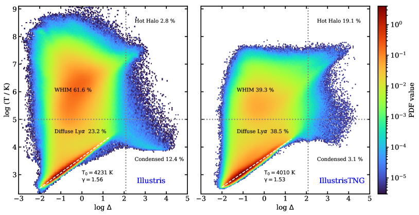
Figure 2: The figure shows the density-temperature distribution of the IGM gas in both Illustris (left panel) and IllustrisTNG (right panel) simulations. The white dashed lines represent the power-law fit to the equation of state of the IGM, $T(\Delta)=T_{0}\Delta^{\gamma-1}$, with the best fit values of $T_{0}$ and $\gamma$ indicated in the legends. Dotted lines at $\Delta=120$ and $T=10^{5}$ K divide the phase diagram into four quadrants, corresponding to different gas phases: diffuse Ly$\alpha$ (cool baryons), WHIM, hot halo gas, and condensed gas. The mass fraction in each phase is also indicated in the legends (see also Table 2).

The parameters governing the feedback prescriptions in galaxy formation simulations are often adjusted to match various observations, and Illustris and IllustrisTNG are no exceptions. The observations used for guiding these adjustments in Illustris and IllustrisTNG include the star formation rate density, stellar mass function (Pillepich et al., 2018b), galaxy sizes and color distribution (Nelson et al., 2018a), clustering of galaxies (Pillepich et al., 2019), and total gas fraction within a radius of halos $R_{500c}$(e.g Weinberger et al., 2017; Genel et al., 2018). Many of the galaxy formation models and the feedback parameters are different for these simulations (see Pillepich et al., 2018a). In fact, the new feedback parameters and prescriptions were implemented in the IllustrisTNG simulation in order to overcome a few shortcomings of the Illustris simulation (refer to Figure 4 of Pillepich et al., 2018a) which include the underestimation of the gas fraction present within $R_{500c}$ of massive halos in Illustris. A comprehensive summary of the changes made to the feedback parameters and prescriptions can be found in Table 1 of Pillepich et al. (2018a), with relevant changes briefly mentioned below.

The feedback mechanisms can be divided into two categories: stellar feedback, which is important for low-mass galaxies, and AGN feedback, which is important for high-mass galaxies. In both simulations, AGN feedback is implemented in two modes based on the rate at which gas is accreted onto the central supermassive black hole: the quasar-mode (Springel, 2005; Hopkins et al., 2008; Debuhr et al., 2011), when the black hole is in a high-accretion state and the radio-mode (Croton et al., 2006; Bower et al., 2006; Sijacki et al., 2007), when it is in a low-accretion state. While both simulations use continuous thermal feedback in the quasar-mode, they differ in their implementation of radio-mode feedback. Illustris uses a bubble model (Sijacki et al., 2007) in which a large amount of feedback energy is gathered over some time and then released explosively, driving the gas out of massive halos into the IGM. In contrast, IllustrisTNG uses kinetic wind feedback (Nelson et al., 2019), in which momentum is stochastically imparted to nearby cells from the low-accretion state black hole (see Weinberger et al., 2017). This latter approach has been shown to be effective in reproducing star formation rates, stellar mass functions, and galaxy color distributions for halo masses of $\sim 10^{12}$ M_⊙ without expelling too much gas and becoming inconsistent with total gas fractions within $R_{500c}$ (Nelson et al., 2018b; Pillepich et al., 2018a).

The Illustris and IllustrisTNG simulations offer an ideal opportunity to study the impact of AGN feedback on the gas distribution around galaxy halos and in the IGM, due to their differences in the radio-mode AGN feedback prescriptions as described above. These publicly available large simulations have been run with the same initial conditions, allowing us to identify the same locations and compare the differences in the density and temperature distribution of the gas. One such comparison is illustrated in Fig. 1 where we show slices of the simulation boxes for the distribution of hydrogen density $n_{\rm H}$ and temperature $T$. The slice has a thickness of one grid cell (i.e., $\sim 60$ ckpc). The figure demonstrates that the distribution of $n_{\rm H}$ and $T$ are significantly different, particularly around the nodes of the cosmic web where halos reside. This is mainly due to the different implementations of radio-mode AGN feedback in the two simulations: the explosive feedback in Illustris results in the displacement of hot gas surrounding halos to a larger volume compared to IllustrisTNG. There are only a few regions, far from Illustris halos, where the density and temperature profiles are similar to those in IllustrisTNG (e.g. at the centre of the slice shown in Fig. 1).

The differences in the temperature and density at the nodes of the cosmic web in Fig. 1 are also reflected in the temperature-density phase diagram shown in Fig. 2. It is created by randomly selecting a large number of pixels from the grids of temperature and density data (in terms of overdensity $\Delta$) and plotting a normalized 2D histogram of the mass-weighted temperature and density values. A comparison of the two simulations reveals that Illustris has more gas at high temperatures ($>10^{5}$ K), as expected based on the distribution shown in Fig. 1. To quantify the gas mass in different phases, the phase diagram is divided into four quadrants using the lines $T=10^{5}$ K and $\Delta=120$, following the definition given in Davé et al. (2010). These quadrants represent four standard gas phases: diffuse Ly$\alpha$ gas or cool baryons ($T<10^{5}$ K and $\Delta<120$), warm-hot intergalactic medium or WHIM ($T>10^{5}$ K and $\Delta<120$), hot halo gas ($T>10^{5}$ K and $\Delta>120$), and condensed gas ($T<10^{5}$ K and $\Delta>120$). The condensed gas particles are those that eventually form stars in the galaxy formation simulation. The mass fractions in these four phases for Illustris and IllustrisTNG are shown in Fig. 2 and listed in Table 2. Compared to IllustrisTNG, Illustris has a lower fraction of gas in the diffuse Ly$\alpha$ phase (23.3% versus 38.5%) and a higher fraction in the WHIM (61.6% versus 39.3%), indicating that the more explosive feedback in Illustris effectively heats low-density gas ($\Delta<120$) to high temperatures ($T>10^{5}$ K) reducing the fraction of diffuse Ly$\alpha$ gas and increasing the WHIM.

Table 1: Parameters of cosmology and $T-\Delta$ relation (at $z=0.1$)

Parameters	Illustris	IllustrisTNG
${\Omega_{m}}$	0.2726	0.3089
$\Omega_{\Lambda}$	0.7274	0.6911
$\Omega_{b}$	0.0456	0.0486
$h$	0.704	0.6774
$\sigma_{8}$	0.809	0.8159
$n_{s}$	0.963	0.97
$T_{0}$	4231 K	4010 K
$\gamma$	1.56	1.53

Table 2: Gas mass fraction in different phases at $z=0.1$

Simulations	Diffuse	WHIM	Hot halo	Condensed
	Ly$\alpha$
Illustris	0.232	0.616	0.028	0.124
IllustrisTNG	0.385	0.393	0.191	0.031

The temperature-density phase diagram in the post-H i-reionization era ($z<6$) often exhibits a tight power-law relation, with most of the gas follows $T(\Delta)=T_{0}\Delta^{\gamma-1}$, where $\rm T_{0}$ is the temperature at mean density (i.e at $\Delta=1$) and $\gamma$ is an adiabatic index (Hui & Gnedin, 1997; McQuinn & Upton Sanderbeck, 2016). At high-$z$, about 80% of the gas follows this power-law relation, but at low-$z$ only a small fraction does due to the presence of a significant amount of hot gas in the WHIM phase. Additionally, the gas tracing the power-law relation is more dispersed at low-$z$, as shown by the puffier high-density regions at low-$T$ and $\Delta$ values in Fig. 2. Therefore, it is not straightforward to fit a $T-\Delta$ power-law at low-$z$. To overcome this issue, we use the method presented in Hu et al. (2022). We first select gas with $T<10^{5}$ K and a range of gas overdensity $-1.5<\log\Delta<1$, then divide this region into 15 equispaced $\log\Delta$ bins. For the $i^{\rm th}$ bin, we record $\log\Delta_{i}$ as the median overdensity value and calculate the temperature $\log T_{i}$ at which the marginal distribution $P(\log T|\log\Delta)$ peaks, as well as its “error" $\sigma_{T_{i}}$, which we define to be of half of the temperature range that sets the 16% to 84% percentile ranges. We then fit the $T-\Delta$ power-law relation to ($\log T_{i}$, $\log\Delta_{i}$) using these errors by minimizing the least-square difference. We found that the ${T-\Delta}$ relations in both the Illustris and IllustrisTNG simulations are nearly identical, with $\rm T_{0}$ values of $4231$ K and $4010$ K and $\gamma$ values of $1.56$ and $1.53$, respectively (also noted in Table 1). The power-law fits are illustrated in Fig. 2 by the white dashed lines on the ${T-\Delta}$ phase diagrams. The agreement of the parameters governing the power-laws between the two simulations is perhaps not surprising, since the temperature of the gas following this power-law relation is governed by the photoionization heating from the UV background which is the same in both simulations. But this does indicate that while feedback processes alter the structure of the phase diagram, the ${T-\Delta}$ relation is nevertheless unchanged. Therefore measuring the ${T-\Delta}$ relation at low-$z$ may not provide any interesting clues regarding the feedback (see e.g, Hu et al., 2023).

Despite the similarity in the temperature-density power-law relation, the mass fractions of different gas phases are significantly different in both simulations (see also Viel et al., 2013b). These differences in the ambient IGM (as seen in Fig. 2) and in the temperature and density of gas around the halos (as shown in Fig. 1) hints that we can use the Ly$\alpha$ forest to distinguish between different feedback models. The Ly$\alpha$ forest is sensitive to changes in hydrogen density and temperature, making it a useful tool for understanding the impact of different feedback approaches on the gas surrounding galaxies and in the ambient IGM. We will explore this further in the following sections.

3 Methods to simulate Lyman-$\alpha$ forest

In this section, we will outline the steps we took to generate synthetic Ly$\alpha$ forest spectra and create mock HST-COS data using forward models. We will also discuss our use of automated Voigt profile fitting following Hiss et al. (2018).

3.1 Generating Synthetic Ly$\alpha$ Forest Spectra

In order to generate synthetic Ly$\alpha$ forest spectra, we draw a large number of sightlines (10⁵) through both the Illustris and IllustrisTNG simulations. These sightlines are parallel to the (arbitrarily chosen) $z-$axis and extend from one side of the simulation box to the other. Starting points of these sightlines are chosen at random in the $x-y$ plane. Along these sightlines, we record the values of the temperature $T$, overdensity $\Delta$, and the peculiar velocity component parallel to the line of sight $v_{z}$. In addition to these quantities, we also need to calculate the neutral hydrogen fractions to create the synthetic Ly$\alpha$ forest spectra. We do this by solving for the neutral fraction in ionization equilibrium, taking into account both collisional ionization and photoionization. At every cell along a sightline, we use the values of $T$, $\Delta$, and $\Gamma_{\rm HI}$ to calculate the neutral fractions. We assume a constant value of $\Gamma_{\rm HI}$ for the entire simulation box. The specific values of $\Gamma_{\rm HI}$ used for Illustris and IllustrisTNG simulations are discussed in Section 4.

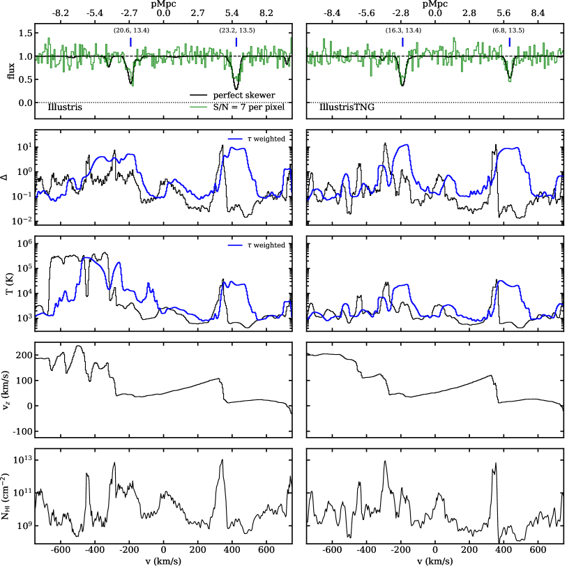
Figure 3: Figure shows an example of a synthetic Ly$\alpha$ forest skewer (a chunk of 1500 km s^-1) from both Illustris (left) and IllustrisTNG (right) simulations. Both skewers are drawn along the same coordinates in both simulations and are shown from top to bottom with the normalized flux, overdensities ($\Delta$), temperature, line of sight velocity ($v_{z}$) and $N_{\rm HI}$ per pixel of the simulation plotted on the y-axis. The green histograms on the top panels show the forward modeled skewers with a signal-to-noise ratio (S/N) of 7 per pixel (6 km s^-1) of the forward model spectra convolved with the HST-COS G130M LSF. The blue ticks indicate the Ly$\alpha$ absorption lines identified by VPfit, with the fitted Doppler widths ($b$ in km s^-1) and column densities ($\log N_{\rm HI}$ in cm^-2) shown in the legend. The blue dashed lines in the second and third panels from the top show the optical depth- weighted overdensities and temperatures, respectively. The different sizes of the skewers in the left and right panels (as noted on the top x-axis) are a result of the different values of the $H_{\rm 0}$ used in the simulations.

To compute the ionization equilibrium, we need the electron density, which has a contribution (up to 16%) from the ionization of helium gas. We approximate the contribution of helium to the electron density by assuming that the helium is doubly ionized i.e. the fractions of He i and He ii are zero. This approximation is justified because the redshift of the simulations is $z=0.1$, which is 10 billion years after the completion of helium reionization ($z\sim 3$; McQuinn et al., 2009; Shull et al., 2010; Worseck et al., 2011; Khaire, 2017). Moreover, this simplifies calculations by removing two extra free parameters, the He i and He ii photoionization rates, from the analysis. Our ionization equilibrium calculations use updated cross-sections and recombination rates from Lukić et al. (2015). In addition, we also use the self-shielding prescription presented in Rahmati et al. (2013) for dense cells.

After determining the neutral fraction of hydrogen, we proceed to generate the simulated optical depth $\tau$, for each cell along the line-of-sight ($z$-axis) by using the $T$ and the velocity component ($v_{z}$). This is achieved by summing the contributions from all real-space cells to the redshift space optical depth, considering the full Voigt profile resulting from each real space cell following Voigt profile approximation given in Tepper-García (2006). The resulting continuum-normalized flux $F$ of the Ly$\alpha$ forest is then obtained by evaluating $F=e^{-\tau}$ along each line of sight. These simulated spectra are referred to as perfect Ly$\alpha$ forest skewers and have a pixel scale of $4.12$ km s^-1 set by the $1820^{3}$ cells used in both simulations. This pixels scale is $\sim 4$ times smaller than the resolution of HST-COS spectra, which have FWHM$\sim 15-20$ km s^-1.

3.2 Forward models for IGM and Voigt profile fitting

To study the IGM in the simulations, we forward model the perfect Ly$\alpha$ forest skewers to generate mock HST-COS Ly$\alpha$ forest spectra with S/N ratio and resolution similar to those presented in Danforth et al. (2016). We use the spectra from Danforth et al. (2016) because it contains the highest S/N low redshift ($z<0.5$) Ly$\alpha$ forest data to date. We mask the spectral regions having metal lines from Milky Way interstellar medium (ISM) and intervening IGM using the line identification provided by Danforth et al. (2016). For this, we follow the same procedures outlined in Khaire et al. (2019). We forward model the Ly$\alpha$ forest in a redshift bin at $0.06<z<0.16$ which is probed by 34 high-quality (S/N per pixel > 10) quasar spectra with a median redshift of the Ly$\alpha$-forest $z=0.1$. To generate these forward models, we randomly stitch together the perfect skewers to match the Ly$\alpha$ forest redshift path of each quasar. We then convolve the flux from the perfect skewers with the lifetime position-dependent HST-COS FUV line spread function for the G130M grating, interpolate it to match the wavelength vectors of the real data (with a velocity pixel scale of $\Delta v\approx 6$ km s^-1), and add Gaussian random noise to each pixel based on the error vectors of the real data.

Once we have generated both perfect skewers and forward-modeled skewers, we use an automated Voigt profile fitting code called VPfit v10.2 (Carswell & Webb, 2014) to decompose each Ly$\alpha$ absorption spectrum into a collection of absorption lines. Each absorption line is described by three parameters: the absorption redshift, the Doppler width ($b$ in km s^-1), and the H i column density ($N_{\rm H\,I}$ in cm^-2). To fit the skewers using VPfit, we use a fully automated Python wrapper that operates VPfit, as described in Hiss et al. (2018, 2019) and also used for analysis in Hu et al. (2022).

For comparison, in Fig. 3 we show a chunk of Ly$\alpha$ forest spectrum generated from a line-of-sight passing through the same spatial coordinates in the Illustris and IllustrisTNG simulations. The choice of $\Gamma_{\rm HI}$ values used for this are explained in section 4. For visualization purposes, the figure shows only a small portion of the spectra ($\pm 750$ km s^-1; $\sim\pm 10$ pMpc) at the center of the simulation box. The top panel shows our forward-modeled skewers as well as the perfect skewers. Blue ticks indicate the locations of Ly$\alpha$ absorption lines automatically identified by VPfit when applied to the forward-modeled skewers, and numbers in the parenthesis indicate the $b$ (km s^-1) and $\log N_{\rm HI}$ (cm^-2) obtained by VPfit. In this example, only two Ly$\alpha$ absorption lines are identified and fitted by VPfit in the small portion of the skewers shown.

The figure also shows temperature and density, and the corresponding optical depth weighted quantities along the skewers. Optical depth weighted overdensities $\Delta^{\tau}_{i}$ and temperatures $T^{\tau}_{i}$ at pixel $i$ are calculated as

$$\Delta^{\tau}_{i}=\frac{\sum_{j=1}^{n}\tau_{ij}\Delta_{j}}{\sum_{j=1}^{n}\tau_{ij}}\quad\&\quad T^{\tau}_{i}=\frac{\sum_{j=1}^{n}\tau_{ij}T_{j}}{\sum_{j=1}^{n}\tau_{ij}},$$ (1)

where $\tau_{ij}$ is the optical depth contribution of real-space pixel $j$ to the total redshift-space optical depth at pixel $i$, and $n$ is the total number of pixels in each spectrum. The optical depth weighted density and temperature are thus redshift space quantities that can be compared directly to the redshift space optical depth.

Since both simulations are run with the same initial conditions, the differences in the $T$, $\Delta$, and line-of-sight velocity ($v_{z}$) along the skewer are the result of the different feedback prescriptions. The temperature and $v_{z}$ panels for the region on the left side of the skewers show that the gas is hotter in Illustris as compared to IllustrisTNG, and the hotter regions of Illustris have steeper velocity gradients as compared to IllustrisTNG. The explosive feedback is partly responsible for the extra velocity kinks seen in the Illustris velocity profile as compared to the smoother one in IllustrisTNG (see $v_{z}$ panel of Fig. 3). The bottom panel of Fig. 3 shows the H i column density at each pixel (of $\sim 60$ kpc) in real space. When the bottom panel is compared to other panels, it illustrates that the high $N_{\rm HI}$ gas ($\gtrsim 10^{13}$) corresponding to high density ($\Delta>3$ ) and lower temperature gas ($T\sim 10^{4}$ K; see the optical depth-weighted density and temperatures) imprints detectable absorption lines on the spectra. Note that the forward modeled spectra shown here are generated using a constant noise vector with a signal-to-noise ratio of 7 per pixel (of $\Delta v\sim 6$ km s^-1).

By running VPfit on these mock spectra we can compare the distribution of $b$ and $N_{\rm HI}$ in both simulations. However, the number of absorption lines and $N_{\rm HI}$ depend on the photoionization rate $\Gamma_{\rm HI}$ from the ionizing UV background radiation. Therefore, when we want to study the effect of feedback on the IGM, $\Gamma_{\rm HI}$ becomes a nuisance parameter that we need to fix for both simulations. In the next section, we will discuss in more detail how to fix this nuisance parameter.

4 Fixing the nuisance parameter $\Gamma_{\rm HI}$

The statistical properties of the IGM, such as the mean flux of the Ly$\alpha$ forest, the flux power spectrum, $b-N_{\rm HI}$ distribution or column density distribution, are important tools for understanding the IGM. These properties depend not only on the temperature-density distribution of the gas in the simulation but also on the $\Gamma_{\rm HI}$ sourced by the UV background. To disentangle the impact of the physical properties of the simulated gas distribution from the impact of the UV background, it is necessary to fix the $\Gamma_{\rm HI}$. This is why it is common practice to consider $\Gamma_{\rm HI}$ as a nuisance parameter and fit for it when analyzing simulated Ly$\alpha$ forest data. To set the value of $\Gamma_{\rm HI}$, simulations must match one or more of the statistical properties of the observed IGM. For example, in high-redshift IGM studies, researchers often use the mean flux in the Ly$\alpha$ forest as a reference. In low-redshifts Viel et al. (2017) used H i column density distribution (CDD; defined in Eq. 3) to tune the $\Gamma_{\rm HI}$. In this work, we have chosen to use the density of Ly$\alpha$ lines defined as the number of Ly$\alpha$ lines per unit redshift interval (${\rm dN/dz}$) as our reference statistic for determining the value of $\Gamma_{\rm HI}$. The range of column densities is chosen to be in between $12<\log\,N_{\rm HI}\,\,({\rm cm}^{-2})<14.5$ for calculating ${\rm dN/dz}$. Matching ${\rm dN/dz}$ is similar to the approach of matching the mean flux or effective Ly$\alpha$ optical depth that is commonly used at higher redshifts ($z>2$). We have chosen not to use the mean flux as a reference because at low redshifts ($z<0.5$), the normalized mean flux in the Ly$\alpha$ forest is very close to unity, and hence uncertainties in the placement of the continuum can have a large impact on its measurement.

To determine the value of $\Gamma_{\rm HI}$ in both simulations, we first obtained the ${\rm dN/dz}$ value from observations. To do this, we fit Voigt profiles to the Ly$\alpha$ forest in 34 quasar spectra in the redshift range of $0.06<z<0.16$ from the dataset of Danforth et al. (2016) having median S/N $\geq 10$ per resolution element. We chose the region of Ly$\alpha$ forest in each spectrum to lie in the rest-wavelength range 1050-1180 Å  to avoid contamination by Ly$\beta$ lines and to remove the quasar’s line-of-sight proximity zone region. Our VPfit code identifies 369 lines in the column density range $12<\log\,N_{\rm HI}\,\,({\rm cm}^{-2})\,<14.5$ over the total Ly$\alpha$ redshift path $\Delta z=1.792$ covered by the data in the aforementioned redshift range. This gives us the number density of Ly$\alpha$ lines ${\rm dN/dz}=205.9$. Using the simulations, we created a large number ($\approx 3500$) of forward modeled Ly$\alpha$ forest spectra for different values of $\Gamma_{\rm HI}$ (from $5\times 10^{-15}$ to $2\times 10^{-13}$ s^-1) following the procedure described in the previous section. We then fit these skewers with the same automated VPfit code, storing the values of $N_{\rm H\,I}$ and $b$ for each Ly$\alpha$ line and determining the ${\rm dN/dz}$ for each $\Gamma_{\rm HI}$.

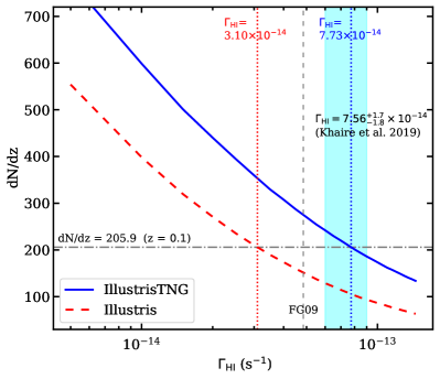
Figure 4: The line density ${\rm dN/dz}$ for Ly$\alpha$ absorbers in the range $10^{12}<N_{\rm HI}<10^{14.5}\,{\rm cm^{-2}}$ is plotted for IllustrisTNG (blue curve) and Illustris (red dashed curve) simulations at $z=0.1$. The grey dot-dashed line shows ${\rm dN/dz}=205.9$, which was obtained by fitting Voigt profiles to the Ly$\alpha$ forest observed in HST COS data from Danforth et al. (2016) in the redshift range $0.06<z<0.16$. The vertical dotted lines indicate the values of $\Gamma_{\rm HI}$ ($3.1\times 10^{-14}$ s^-1 for Illustris and $7.73\times 10^{-14}$ s^-1 for IllustrisTNG) at which the simulations match the ${\rm dN/dz}$ of the data. The cyan-shaded region shows the measurements of $\Gamma_{\rm HI}$ and its 1$\sigma$ uncertainty obtained by Khaire et al. (2019) using Nyx simulations without any feedback. The gray dashed vertical line shows the $\Gamma_{\rm HI}$ at $z=0.1$ from Faucher-Giguère et al. (2009) used by both Illustris and IllustrisTNG. This figure demonstrates that Illustris, which has explosive feedback and a small fraction of gas mass in the diffuse Ly$\alpha$ phase, requires a lower value of $\Gamma_{\rm HI}$ to match the observed ${\rm dN/dz}$.

In Fig. 4, we present the values of ${\rm dN/dz}$ obtained for various $\Gamma_{\rm HI}$ values in both IllustrisTNG and Illustris simulations. The horizontal line, indicating our measurement of ${\rm dN/dz}=205.9$ from the data, serves as a reference for comparison. Our results show that IllustrisTNG requires $\Gamma_{\rm HI}=7.73\times 10^{-14}$ s^-1 to match this measurement, while Illustris requires $\Gamma_{\rm HI}=3.1\times 10^{-14}$ s^-1 (as indicated by the vertical dotted lines in Fig. 4). We use these $\Gamma_{\rm HI}$ values for comparing the results of Illustris and IllustrisTNG throughout this paper. Note that the example skewer shown in Fig. 3 has been calculated for these values of $\Gamma_{\rm HI}$ only.

Here we have used ${\rm dN/dz}$ in $12<{\rm log}N_{\rm HI}\,\,({\rm cm}^{-2})<14.5$ range for tuning the $\Gamma_{\rm HI}$. However, if we choose a small interval $13<{\rm log}N_{\rm HI}\,\,({\rm cm}^{-2})<14.5$ which is unaffected by the incompleteness of line identifications in Danforth et al. (2016), we get $\Gamma_{\rm HI}$ that is 15% higher than those obtained here. Instead of using ${\rm dN/dz}$ for tuning $\Gamma_{\rm HI}$ one can use either mean flux or H i CDD. These are all valid approaches (see e.g Viel et al., 2017; Bolton et al., 2022b) however one needs to be cautious while using mean flux at low-$z$ because it is very close to 1 where the noise as well as the continuum placement uncertainty can severely affect its measurements. Instead of $\rm dN/dz$ if we use the mean flux for tuning $\Gamma_{\rm HI}$, calculated as the mean of the continuum normalized flux in the Ly$\alpha$ forest region excluding the metal lines in the same redshift bin $0.6<z<0.16$, we obtain $\Gamma_{\rm HI}$ values that are within 5% of those obtained using $\rm dN/dz$. In Section 5.2, we demonstrate that our $\Gamma_{\rm HI}$ values obtained through ${\rm dN/dz}$ matching yield CDD consistent with observations within the same $12<{\rm log}N_{\rm HI}\,\,({\rm cm}^{-2})\,<14.5$ range used ${\rm dN/dz}$ (see Fig. 8). Alternatively, if we use the CDD within the $13<{\rm log}N_{\rm HI}\,\,({\rm cm}^{-2})\,<14.5$ range, we find that the resulting values of $\Gamma_{\rm HI}$ for both simulations are within 10% of those obtained using ${\rm dN/dz}$ for the same $N_{\rm HI}$ range. Therefore we conclude that, for the purpose of calibrating $\Gamma_{\rm HI}$, the use of ${\rm dN/dz}$ is equivalent to using mean flux or CDD.

Given that the mass fraction in the diffuse Ly$\alpha$ phase is quite different in the Illustris and IllustrisTNG simulations, we expect the $\Gamma_{\rm HI}$ values to be different in order to match the ${\rm dN/dz}$. This is a result of the fact that most of the summary statistics of the Ly$\alpha$ forest (e.g. mean flux, CDD or $\rm dN/dz$) are related to the mean effective Ly$\alpha$ optical depth $\tau$ which can be approximated as,

$$\tau\propto\Gamma_{\rm HI}^{-1}\,T^{-0.7}_{0}({\rm f_{Ly\alpha}}\,\Omega_{b}\,h^{2})^{2}\,\Omega_{m}^{-0.5},$$ (2)

following the fluctuating Gunn-Peterson approximation (Weinberg et al., 1997) where ${\rm f_{Ly\alpha}}$ is the fraction of mass in the diffuse Ly$\alpha$ phase (see Fig. 2). As expected from Eq. 2, the required $\Gamma_{\rm HI}$ for Illustris is smaller than IllustrisTNG because of the lower ${\rm f_{Ly\alpha}}$. The expected ratio of $\Gamma_{\rm HI}$ values of IllustrisTNG relative to Illustris (using Eq. 2) is a factor of $2.52$ when we demand that the mean optical depths of both simulations should be the same and use the ${\rm f_{Ly\alpha}}$ and cosmological parameters from table 1 and 2. Note that most of the difference arises from the ${\rm f_{Ly\alpha}^{2}}$ factor. The ratio of $2.49$ that we obtained by by ${\rm dN/dz}$ matching is in excellent agreement with the expectation from this scaling argument based on the fluctuating Gunn-Peterson approximation.

Note that Illustris and IllustrisTNG used the Faucher-Giguère et al. (2009) UV background which gives $\Gamma_{\rm HI}=4.85\times 10^{-14}$ s^-1 at $z=0.1$ as indicated by gray dashed vertical line in Fig. 4. Assuming this value of $\Gamma_{\rm HI}$, Illustris under-predicts the measured ${\rm dN/dz}$ by $26\%$ and IllustrisTNG over-predicts it by $34\%$.

In Khaire et al. (2019), we measured $\Gamma_{\rm HI}$ to be $7.56^{{}^{+1.7}_{-1.8}}\times 10^{-14}$ s^-1 at $z=0.1$ (as shown by the cyan shade in Fig.4). For this measurement, we compared a measurement of the Ly$\alpha$ forest flux power spectrum to an ensemble of Nyx simulations (Almgren et al., 2013), which do not model galaxy formation or feedback. This value of $\Gamma_{\rm HI}$ is consistent with the value needed to match the ${\rm dN/dz}$ measurement for IllustrisTNG, but $2.5\,\sigma$ higher than the value needed for Illustris. This consistency between the Nyx and IllustrisTNG $\Gamma_{\rm HI}$ is not surprising, as the diffuse Ly$\alpha$ fraction in the Nyx simulation (39.3%) is only 1% higher than in IllustrisTNG (see Hu et al., 2023).

By utilizing the simple statistical measure ${\rm dN/dz}$ to fix the nuisance parameter $\Gamma_{\rm HI}$, we have demonstrated that the ${\rm dN/dz}$ depends on $f_{\rm Ly\alpha}^{2}$/$\Gamma_{\rm HI}$, akin to the mean Ly$\alpha$ effective optical depth. This degeneracy between $f_{\rm Ly\alpha}$ and $\Gamma_{\rm HI}$ is critical to comprehend the relationship between feedback and the inferred $\Gamma_{\rm HI}$. If feedback removes gas from the diffuse Ly$\alpha$ phase by heating it to a higher temperature, thereby reducing $f_{\rm Ly\alpha}$, then the inferred $\Gamma_{\rm HI}$ needed to match the ${\rm dN/dz}$ will also decrease. This scenario is observed in simulations with extreme feedback, such as Illustris, which has a $f_{\rm Ly\alpha}$ of just $23$% (see Table 2), compared to the $38$% of IllustrisTNG. Therefore, we require different values of $\Gamma_{\rm HI}$ to compare the IGM from both simulations.

After adjusting the nuisance parameter $\Gamma_{\rm HI}$, we proceed to examine the impact of feedback on the Ly$\alpha$ forest in both simulations. Our findings will be presented and discussed in the following section.

5 Quantifying the Impact of Feedback on IGM Statistics

We investigate the impact of feedback on the IGM by comparing a variety of statistics, including the $b$-distribution, the $N_{\rm H\,I}$-distribution, the joint $b-$$N_{\rm H\,I}$ distribution, the column density distribution function, and the flux power spectrum. The results of these are described below.

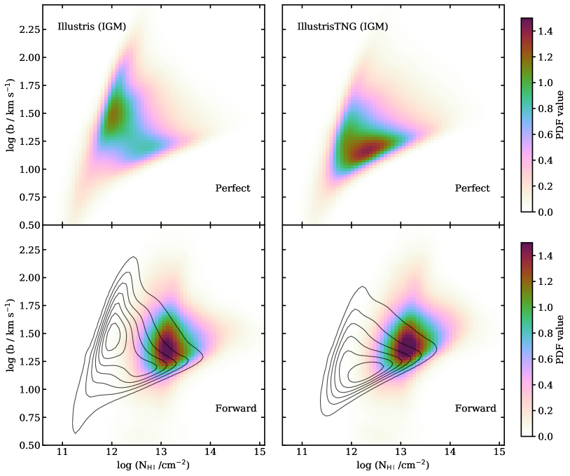
Figure 5: The $b$-$N_{\rm H\,I}$ distributions for Illustris (left panel) and IllustrisTNG (right panel) are shown for perfect IGM skewers (top panels) and forward-modeled Ly$\alpha$ spectra (bottom panels). For better visual comparison, the contours of the perfect $b$-$N_{\rm H\,I}$ distributions are also included in the bottom panels. The effect of feedback can be seen in the different shapes of the perfect $b$-$N_{\rm H\,I}$ distributions (top-panels). The hotter gas in Illustris results in more gas at high $b$ low $N_{\rm H\,I}$ values, while the slightly cooler gas in IllustrisTNG results in lower $b$ high $N_{\rm H\,I}$ values. However, the $b$-$N_{\rm H\,I}$ distributions for forward-modeled Ly$\alpha$ spectra are similar for both simulations. The difference seen in the perfect models is not present in the forward modeled $b$-$N_{\rm H\,I}$. This is because the forward-modeled spectra are not sensitive to these lower $N_{\rm H\,I}$ values where perfect models show the difference.

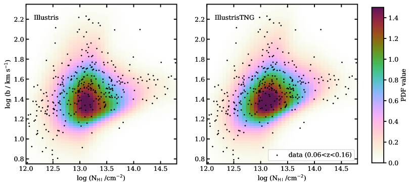
Figure 6: The $b$-$N_{\rm H\,I}$ distribution from forward modelled Ly$\alpha$ forest (as shown in the bottom panel of Fig. 6) for Illustris (left) and IllustrisTNG (right) along with the $b$-$N_{\rm H\,I}$ values obtained by Voigt profile fitting the Ly$\alpha$ forest observed in HST COS data from Danforth et al. (2016) in a redshift bin $0.06<z<0.16$. Both simulations under-predict the $b$ values (see also Fig. 7 for separate $b$ and $N_{\rm H\,I}$ distribution).

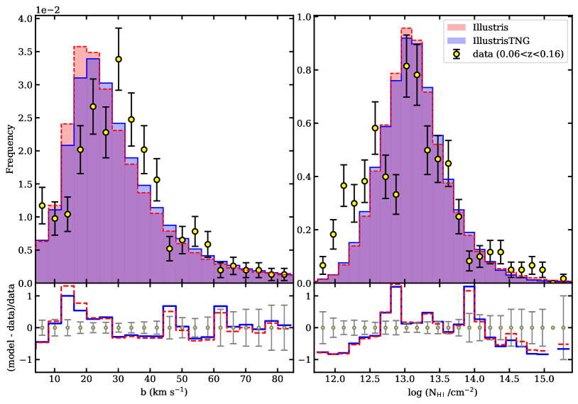
Figure 7: Normalized distribution of $b$ (left-hand panel) and $N_{\rm H\,I}$ (right hand panel) for forward modelled Ly$\alpha$ forest skewers from Illustris (reds-dash histogram) and IllustrisTNG (blue histogram). Forward models from both simulations provide similar $b$ and $N_{\rm H\,I}$ distributions. Data points show the normalized $b$ and $N_{\rm H\,I}$ distribution obtained by fitting the Ly$\alpha$ forest in Danforth et al. (2016) data in a redshift bin $0.06<z<0.16$. The bottom panel shows the fractional difference between the histograms from simulations and the data, while error bars show the the fractional difference in the uncertainty of the data. Both simulations fail to reproduce the $b$ distribution at $b\lesssim 45$ km s^-1 and $N_{\rm H\,I}$ distribution at low ($N_{\rm H\,I}$$\,<10^{12.5}$ cm^-2) and high $N_{\rm H\,I}$($\,>10^{14.5}$ cm^-2).

5.1 The $b-$$N_{\rm H\,I}$ distribution

To obtain the $b-$$N_{\rm H\,I}$ distribution from simulations, we need to Voigt profile fit the mock Ly$\alpha$ forest spectra created from those simulations. However, the automated Voigt profile fitting code, VPfit, does not work well on the perfect, noiseless skewers. This is mainly because VPfit tries to identify absorption lines in regions that are bounded by flux equal to the continuum. However, for most of the redshift path, the continuum normalized flux is slightly below unity due to the highly ionized IGM at low redshifts. As a result, VPfit fails to identify and fit the lines in these regions. To mitigate this issue, as done previously in Hiss et al. (2018) and Hu et al. (2022), we add Gaussian random noise to the flux of the perfect skewers so that the S/N per pixel ($\Delta v=4.1$ km s^-1) is equal to 100 (the equivalent of $\sim 200$ per resolution element for HST COS spectrum). This allows VPfit to accurately identify Ly$\alpha$ lines and fit to obtain $b$ and $N_{\rm H\,I}$ for each line.

We ran VPfit on $10^{5}$ perfect skewers (after adding a tiny amount of noise as mentioned above) and obtain the values of $b$ and $N_{\rm H\,I}$. Using these values, we compute a Kernel Density Estimate (KDE) of the joint $b-$$N_{\rm H\,I}$ distribution using a Gaussian kernel, which is shown in the top panels of Fig. 5 for Illustris (left panel) and IllustrisTNG (right panel). Clear differences can be seen in the shape of the $b$-$N_{\rm H\,I}$ distribution. In Illustris, most of the lines fall in the low column density ($N_{\rm H\,I}$$<10^{12.3}$ cm^-2) region with higher $b$ values ($b>$ 18 km s^-1). In contrast, in IllustrisTNG, the gas is distributed more uniformly across the $b-$$N_{\rm H\,I}$ plane, with more gas at high column densities ($N_{\rm H\,I}$$>10^{11.8}$ cm^-2) and low $b$ values ($b<$ 20 km s^-1). The differences in the $b$ values indicate that the Ly$\alpha$ absorbing gas is hotter in Illustris compared to IllustrisTNG. However, differences in the column densities, where IllustrisTNG shows more gas at slightly higher column densities than Illustris, are not significant, as they are expected to be similar due to the way we fixed the values of $\Gamma_{\rm HI}$. It is interesting to see that, even after fixing the nuisance parameter $\Gamma_{\rm HI}$ to give the same $\rm dN/dz$, the effect of feedback is clearly seen in the shape of the $b-$$N_{\rm H\,I}$ distribution of the perfect skewers. Therefore, ideally one can use very high S/N spectra ($\sim 100$ per pixel) and resolution ($\sim 4.1$ km s^-1) for constraining the effect of feedback on the IGM, however unfortunately only a small fraction of data would exist close to this S/N and resolution (e.g. using the Space Telescope Imaging Spectrograph).

To determine whether the differences in the $b$-$N_{\rm H\,I}$ distribution observed in the perfect skewers can be detected in real data, we conducted the same analysis on our forward-modeled mock spectra. We created these models using the noise properties of Danforth et al. (2016) for the same $10^{5}$ perfect skewers. On average, we needed to stitch around three skewers together for each forward-modeled spectrum, resulting in a total of approximately 35,000 forward-modeled spectra. In contrast to the noiseless perfect skewers, VPfit works well on these forward models because of the noise. The KDEs of the joint $b-$$N_{\rm H\,I}$ distribution from these forward models are shown in the bottom panels of Fig. 5 for Illustris (left panel) and IllustrisTNG (right panel). The figure shows that the differences between the two simulations that were present in the $b-$$N_{\rm H\,I}$ distribution of the perfect skewers (shown in the lower panels of Fig. 5 by contours) are completely washed out in the forward models. The joint $b-$$N_{\rm H\,I}$ distribution looks similar for both Illustris and IllustrisTNG, which is mainly because only the low column density systems ($10^{11.5}<\,$$N_{\rm H\,I}$$\,<10^{13.2}$ cm^-2) showed differences in the case of the perfect skewers. These low-column density lines are not detected in the forward modeled HST/COS spectra given the lower S/N and moderate resolution ($R\sim 15000-20000$). The normalization of the joint $b-$$N_{\rm H\,I}$ distribution (as indicated by color-bar) is also the same for both simulations, as expected due to our choice of $\Gamma_{\rm HI}$ to match ${\rm dN/dz}$. This suggests that even the best available dataset of low-$z$ Ly$\alpha$ forest, as provided in Danforth et al. (2016), can not probe the effects of feedback on the IGM using the $b-$$N_{\rm H\,I}$ distribution.

To further explore this, in Fig. 6, we compare the $b-$$N_{\rm H\,I}$ distribution from Illustris and IllustrisTNG with the observations in the $0.06<z<0.16$ bin that we fit using the same automated VPfit code. The data appears to agree reasonably well with both simulations in terms of $N_{\rm H\,I}$, but observations show an excess of lines with higher $b$ values. To further investigate this discrepancy, we plot the normalized marginalized histograms of $b$ and $N_{\rm H\,I}$ in Fig. 7. It can be seen that both simulations fail to match the $b$ distribution, with peaks at $b\approx 20$ km s^-1 for Illustris and IllustrisTNG, while the peak in the data appears at $b\approx 30$ km s^-1. Previous studies (Viel et al., 2017; Gaikwad et al., 2017b; Nasir et al., 2017) have also noted this discrepancy in $b$ values, which has been argued to indicate a hotter IGM or some effect of feedback or other possible sources of additional heating such as from dark photon dark matter (see Bolton et al., 2022a). However, even in the case of extreme feedback in Illustris, the discrepancy remains. It seems that Illustris even gives a slightly smaller peak in $b$ than IllustrisTNG, although the difference is not significant. However, it does not definitively mean that feedback can not affect the $b$ distribution and it might be that feedback models implemented in both Illustris and IllustrisTNG simulations are lacking some ingredients to reproduce the observed $b$ distribution. On the other hand, by construction given the ${\rm dN/dz}$ matching, both simulations give almost identical $N_{\rm H\,I}$ distributions in the $12<{\rm logN_{HI}}\,\,({\rm cm}^{-2})<14.5$ range. There is a mild disagreement around two bins centered at log $N_{\rm H\,I}$ $\approx 12.7$ and $13.3$ where both simulations overproduce the number of Ly$\alpha$ lines. At higher column densities (log $N_{\rm H\,I}$ $>15$) simulations under-produce Ly$\alpha$ lines.

In summary, we find that Illustris and IllustrisTNG exhibit different $b-$$N_{\rm H\,I}$ distributions, however, the existing data does not have a sufficiently high S/N ratio and resolution to discern this difference. Both simulations are also unable to reproduce the discrepancy between the observed and simulated $b$ distributions at low redshifts. This suggests the need for further investigation into the issue of the $b$ distribution (see Bolton et al., 2022b, a).

5.2 The column density distribution

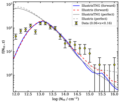
Figure 8: The figure shows the $z=0.1$ H i column density distribution (CDD) for Illustris (dashed curves) and IllustrisTNG (solid curves) simulations when we use perfect and forward-modeled skewers. We also show the CDD obtained by fitting the Danforth et al. (2016) data at $0.06<z<0.16$ bin using our VPfit code. The simulations show good agreement with each other at log $N_{\rm H\,I}$$\lesssim\,14.5$ but diverge at higher column densities. In forward models, both simulations are consistent with CDD measurement at $12.3<\log\,N_{\rm HI}<14.5$ but under-predict it at higher column densities, with IllustrisTNG showing a greater under-prediction than Illustris.

We calculate the H i CDD defined as

$$f(N_{\rm HI},z)=\frac{d^{2}N}{d\log N_{\rm HI}\,dz},$$ (3)

where $N$ is the number of Ly$\alpha$ absorption lines with H i column density in the range $\log N_{\rm HI}$ to $\log N_{\rm HI}$ + $\Delta\log N_{\rm HI}$ detected within the observed redshift pathlength $dz$. We calculate the CDD for perfect skewers as well as forward-modeled skewers for both simulations. The results are shown in Fig. 8.

Fig. 8 shows that both simulations give identical CDDs for $\log N_{\rm HI}\lesssim 14.5$ for perfect skewers (gray curves) as well as forward-modeled skewers (blue and red curves). This is not surprising given our method of fixing the nuisance parameter $\Gamma_{\rm HI}$. The CDDs of Illustris and IllustrisTNG begin to deviate from each other at $\log N_{\rm HI}\,\,({\rm cm}^{-2})\gtrsim 15$ and $\log N_{\rm HI}\,\,({\rm cm}^{-2})\gtrsim 14.3$ where Illustris gives higher CDD than IllustrisTNG for perfect skewers and forward-modeled skewers, respectively. This small deviation may be related to the feedback prescriptions as well as how VPfit fits noisy, saturated lines. Given that Illustris generally has more shock-heated gas than IllustrisTNG, the lines are wider in Illustris and therefore saturate at slightly higher column densities than for Illustris. This leads to more lines and hence a higher CDD at higher column densities for Illustris compared to IllustrisTNG. According to this argument if the data has an overall higher S/N then the $N_{\rm HI}$ above which the CDD deviates in both simulations would be higher. This is what is seen in the case of the perfect skewers that have S/N of 100 per pixel (of size $4.1$ km s^-1, because of added noise to the spectra) as compared to forward models. There is also a small difference in the CDD of Illustris and IllustrisTNG at lower column densities ($N_{\rm H\,I}$ $<10^{12.5}$ cm^-2) for perfect skewers. This difference is too small to be detected in a realistic dataset and becomes even smaller for the forward model spectra.

Fig. 8 depicts a notable decrease in the CDD at $\log\,N_{\rm HI}\lesssim 13$ for forward-modeled skewers as opposed to perfect skewers. This reduction is attributed to the undetected lower column density Ly$\alpha$ lines that are obscured by the noise. Consequently, noisy forward-modeled skewers yield lower CDD values in comparison to perfect skewers (with S/N = 100 per pixel of size $4.1$ km s^-1). The minimum column density at which the downturn occurs depends on the overall S/N ratio of the data. In typical CDD measurements, such as those conducted by Danforth et al. (2016), this downturn is often corrected by a completeness correction that accounts for the number of lines that can be missed in the noisy data. As we forward model the spectra using the real data, we can conduct a direct comparison of the CDD with observations, rendering such completeness correction unnecessary.

In Fig. 8 we also show the CDD that we obtain by fitting the Danforth et al. (2016) Ly$\alpha$ forest in the $0.06<z<0.16$ bin. The CDD is calculated in bins of $\Delta\log\,N_{\rm HI}=0.2$, and errors on CDD only account for the Poisson counting errors (i.e $\sqrt{N}$) on the number of lines in each bin. If there are no lines in the bin then the upper limit on the confidence interval in counting lines is taken as 1. Since, as mentioned earlier, we will be comparing it with our forward models, we do not need to perform a completeness correction. As expected, our forward-modeled CDD in both simulations matches well with observations in $12<\log N_{\rm HI}\,\,({\rm cm}^{-2})<14.5$ range. At higher column densities both simulations under-predict the CDD. It is worth noting that Illustris provides a better fit to the data than IllustrisTNG at higher column densities $14<\log N_{\rm HI}\,\,({\rm cm}^{-2})<15$. However, this tiny improvement in fitting the CDD can not be treated as definitive evidence that the feedback model in Illustris is closer to reality than IllustrisTNG.

Overall, we conclude that the CDD from Illustris and IllustrisTNG simulations does not show any clear evidence of the effect of feedback on the IGM at $\log N_{\rm HI}\,\,({\rm cm}^{-2})\lesssim 15$. There is a small variation in the CDD at $\log N_{\rm HI}\,\,({\rm cm}^{-2})\gtrsim 15$, which may suggest that the explosive feedback in Illustris is responsible for the higher CDD. However, the difference between the simulations and data is not significant enough to favor any particular feedback model.

It is important to note that a large difference in the CDD, especially in its normalization, can be observed if $\Gamma_{\rm HI}$ is not calibrated. This could be misinterpreted as a potential observable to differentiate between feedback models (see for e.g Burkhart et al., 2022, and discussion in section 6). But because we cannot predict $\Gamma_{\rm HI}$ from first principles, it must be treated as a nuisance parameter that can be fixed by matching the ${\rm dN/dz}$. Any comparison with observational data would be inaccurate if the degeneracy stemming from $\Gamma_{\rm HI}$ is not resolved. The only relevant aspect of the CDD for determining the best feedback models may be its shape, which is mostly independent of the value of $\Gamma_{\rm HI}$.

5.3 The Ly$\alpha$ Flux Power Spectrum

The Ly$\alpha$ flux power spectrum is a widely-used statistical measure for studying the IGM. It has been employed to determine the temperature of the IGM (e.g Theuns et al., 2000; Boera et al., 2019; Walther et al., 2019; Gaikwad et al., 2021) and the UV background (e.g Gaikwad et al., 2017a; Khaire et al., 2019), as well as to constrain cosmological parameters such as neutrino masses (e.g McDonald et al., 2006; Yèche et al., 2017) and to probe alternative dark matter models such as warm or fuzzy dark matter (Viel et al., 2013a; Irsic et al., 2017) at high redshifts. In order to investigate whether the Ly$\alpha$ flux power spectrum can be used to study the effect of feedback on the IGM, we compute it using $10^{5}$ perfect skewers from Illustris and IllustrisTNG. We first calculate the flux contrast, $\delta_{F}=(F-\bar{F})/\bar{F}$, and then compute the Fourier transform, $\hat{f}(k)$, of $\delta_{F}$. The power spectrum is then defined as $P(k)\propto\,\mid\hat{f}(k)\mid^{2}$ with standard normalization $\sigma^{2}_{\delta_{F}}=\int_{-\infty}^{\infty}{dk\,P(k)/2\pi}$.

In Fig. 9, we present the power spectrum ($kP(k)/\pi$) at $z=0.1$ calculated using the noiseless perfect skewers for both Illustris and IllustrisTNG in the top panel, and the percentage difference between them in the bottom panel. The minimum wavenumber $k$ probed by the power spectrum is determined by the size of the skewers, which in this case is the size of the simulation box. At large scales ($k<0.02$ s km^-1), the power spectra from both simulations show good agreement. However, they begin to diverge at smaller scales ($k>0.02$ s km^-1) where Illustris exhibits higher power than IllustrisTNG. The difference between the two simulations is approximately 5% for $k<0.02$ s km^-1 and increases monotonically at higher $k$ values. This difference is likely due to the impact of feedback on the IGM in the simulations. We compare the measurement uncertainties from the power spectrum measurements at $z=0.1$ by Khaire et al. (2019) with this difference in the bottom panel of Fig. 9. It shows that only at $k>0.04$ s km^-1 is the difference in the simulations more than the measurement uncertainties. Therefore, the difference in the power spectrum at small scales (i.e. $k>0.02$ s km^-1) may indicate the effect of feedback. However, note that at these $k$ values, the noise power from the data begins to dominate the power spectrum measurements (see magenta diamonds in the top panel).

Power spectrum measurements at $z=0.1$ plotted in Fig. 9 are from our previous work Khaire et al. (2019) where we used the same dataset and redshift bin for Danforth et al. (2016) data to obtain the power spectrum. Contrary to our expectation, the power spectra from both simulations do not match the measurements at the large scales ($k<0.02$ s km^-1). The simulated power spectra on average under-predict the measurement at these scales by a factor of $\sim 1.5$. This huge discrepancy is surprising and unexpected.

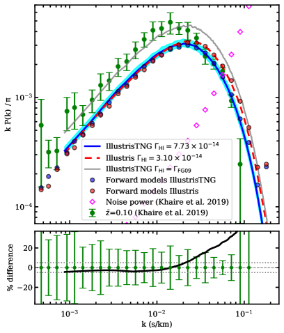
Figure 9: Figure shows line of sight Ly$\alpha$ flux power spectrum ($kP(k)/\pi$) obtained using perfect skewers from IllustrisTNG (blue curve) and Illustris (red-dash) at $z=0.1$ for the $\Gamma_{\rm HI}$ values obtained by matching ${\rm dN/dz}$ along with the measurements (green data points) and the noise power (magenta diamonds) from Khaire et al. (2019). The red and blue circles show the power spectrum calculated from forward modeled HST-COS spectra for Illustris and IllustrisTNG, respectively, following the same procedure employed for measurements in Khaire et al. (2019). The bottom panel shows the relative percentage difference (black curve) in the power spectrum of Illustris (red-dash) with respect to IllustrisTNG (blue solid) and the error bars show percentage errors in the measurements where dotted horizontal lines are for $\pm 5$%. The discrepancy between simulations and measurements is discussed in Section 5.3. For comparison, we show the power spectrum from IllustrisTNG at the $\Gamma_{\rm HI}$ values of Faucher-Giguère et al. (2009), i.e $\Gamma_{\rm FG09}=4.85\times 10^{-14}$ s^-1 (grey solid curve). The cyan shade corresponds to the range of power-spectrum from IllustrisTNG perfect skewers, when we take into account the Poisson error on $\rm dN/dz$ to obtain the $\Gamma_{\rm HI}$.

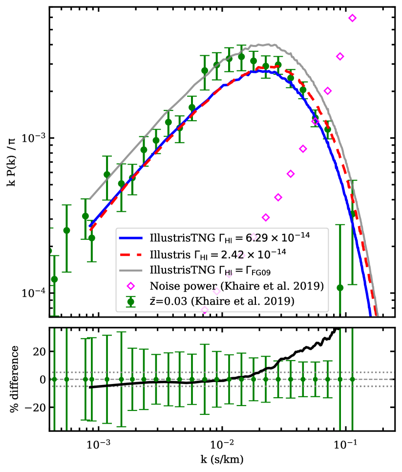
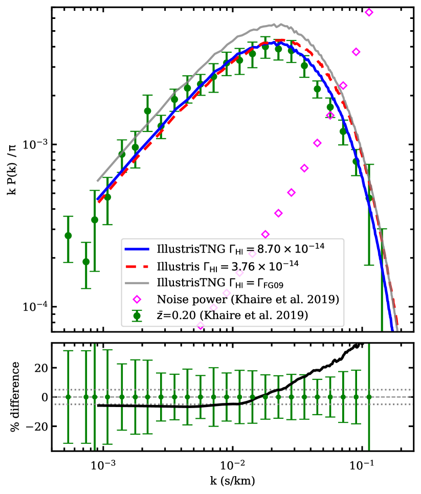
Figure 10: Figure shows line of sight Ly$\alpha$ flux power spectrum obtained using perfect skewers from IllustrisTNG (blue curve) and Illustris (red-dash) at $z=0.03$ (left-hand panel) and $z=0.2$ (right-hand panel) for the $\Gamma_{\rm HI}$ values (as indicated in the legends) obtained by ${\rm dN/dz}$ matching. At these redshifts, the simulated power spectrum is consistent with measurements. The curves and the description of the figure are the same as Fig. 9 and $\Gamma_{\rm FG09}$ is $3.97\times 10^{-14}$ s^-1 for $z=0.03$ and $6.38\times 10^{-14}$ s^-1 for $z=0.2$.

To investigate whether this discrepancy is because of not considering uncertainty in the values of $\Gamma_{\rm HI}$ when we match $\rm dN/dz$ (see Fig. 4), we estimate the 1-$\sigma$ lower and upper bounds on the $\Gamma_{\rm HI}$ by taking Poisson error on the measured $\rm dN/dz=209.5\pm 14.9$. Then by matching $\rm dN/dz$ we find $\Gamma_{\rm HI}=7.73^{+0.87}_{-0.75}\times 10^{-14}$ s^-1 for IllustrisTNG. For this range of $\Gamma_{\rm HI}$ we estimate flux power and plot it as a cyan shade in the Fig. 9, which is still well below the measurements. Nevertheless, incorporating this uncertainty fails to resolve the discrepancy between the data and the models; instead, it shows that the discrepancy is quite severe.

We further investigated whether the observed discrepancy could be attributed to the computation of power using perfect skewers, thereby neglecting the influence of real noise, window function corrections associated with the COS line spread function, and metal line masks used in power spectrum calculations from observational data (as in Khaire et al., 2019). To address this, we employed our forward models, consisting of $\approx 35000$ spectra, with metal masks positioned identically to those in the actual data. The power spectrum was then computed with appropriate window corrections, employing the Lomb-Scargle periodogram (Lomb, 1976; Scargle, 1982) to handle the masked spectra, in accordance with the methods employed in (Khaire et al., 2019; Walther et al., 2018), for both the Illustris and IllustrisTNG forward models. The results, depicted in Fig. 9 as red (Illustris) and blue circles (IllustrisTNG), reveal that these forward-modeled power spectra closely resemble the one obtained with perfect skewers. Thus, the observed discrepancy can not be attributed to the use of perfect versus forward-modeled spectra or the algorithms employed for power spectrum calculations.

To determine if the discrepancy between the measured power spectrum and the simulated power spectrum, for the values of $\Gamma_{\rm HI}$ obtained by matching the $\rm dN/dz$, exist at other redshifts, we conducted the same analysis at two other redshifts $z=0.03$ and $0.2$. We generated forward-modeled skewers from simulation snapshots at $z=0.03$ and $z=0.1$ for different values of $\Gamma_{\rm HI}$ and used VPfit to fit these skewers and the Danforth et al. (2016) data in the respective redshift bins. We then estimated $\Gamma_{\rm HI}$ by matching model $\rm dN/dz$ values at both redshifts with $\rm dN/dz$ from observed data (see Fig. 11 in the Appendix). For these $\rm dN/dz$ matched values of $\Gamma_{\rm HI}$, we computed the power spectra from perfect skewers and compared with our measurements from Khaire et al. (2019). The results are shown in Fig. 10. Note that since the power spectrum from forward-modeled Ly$\alpha$ forest matches closely with the one computed with perfect skewers (as shown in Fig. 9), we do not show the forward-modeled power spectrum in Fig. 10. At $z=0.03$ and $0.2$, the simulated power spectra match well with the measured power spectra. There is no indication of the large discrepancy as seen for $z=0.1$. In fact, the reason behind the discrepancy seen here at $z=0.1$ is because of non-monotonically increasing $\rm dN/dz$ with redshift. The values of $\rm dN/dz$ for $z=0.03$ and $0.1$ and $0.2$ are $227.5$, $205.9$ and $284.9$, respectively. The $\rm dN/dz$ decreases at $z=0.1$ as compared to $z=0.03$ whereas higher values of $\rm dN/dz$ at $z=0.1$ would have reduced the discrepancy. All of these suggest that there may be an issue with the measured power spectrum or $\rm dN/dz$ at $z=0.1$. To investigate this we conducted various tests and rechecked our calculations performed in Khaire et al. (2019) with different data sets and processing of the data, but we were unable to resolve the problem. We have also noted a similar discrepancy in the case of NyX simulations. This problem at $z=0.1$ warrants further investigation of the power spectrum measurement and perhaps $\rm dN/dz$ measurement in order to fully understand the nature of the disagreement between simulations and observations.

However, when comparing the power spectra at all three redshifts from Illustris and IllustrisTNG, we observe good agreement (within 5%) at large scales ($k<0.02$ s km^-1), but noticeable differences arise at smaller scales. This indicates that the small-scale power spectrum ($k>0.02$ s km^-1) is indeed sensitive to the feedback prescriptions used in the simulations. The reason behind the difference is perhaps because of the relatively strong feedback model employed by Illustris. Nevertheless, it is important to note that the magnitude of this difference is not significantly large, and at even smaller scales ($k>0.05$ s km^-1), the noise power dominates the measurements. But a more glaring discrepancy is in the measurements and the predictions at $z=0.1$ power spectrum. To address this discrepancy and further explore the sensitivity of the power spectrum to feedback at small scales, we intend to conduct thorough investigations in future work.

It is also worth noting that the feedback introduces variations in the power spectrum at small scales ($k>0.02$ s km^-1) of around 4-5%. This could potentially introduce additional degeneracies when attempting to measure the thermal state of the IGM at low redshifts. While the effect of feedback is expected to diminish at higher redshifts ($z>2$), it may still be necessary to consider the small percentage level differences in the power spectrum resulting from feedback when using the high-$z$ Ly$\alpha$ power spectrum to obtain precise cosmological parameters, as indicated by Chabanier et al. (2020).

We also show the power spectrum for the IllustrisTNG simulation using the Faucher-Giguère et al. (2009) UV background at three different redshifts: $z=0.1$, $z=0.03$, and $z=0.2$ in Fig. 9 and 10. In Fig. 9, we verify the findings of Burkhart et al. (2022) that the IllustrisTNG power spectrum at $z=0.1$ calculated for Faucher-Giguère et al. (2009) UV background is consistent with measurements. However, upon inspecting the power spectrum at the other redshifts (as shown in Fig. 10), we observe that it is significantly higher than the measurements for most $k$ values. This implies that the match between the IllustrisTNG power spectrum and measurements at $z=0.1$ using the Faucher-Giguère et al. (2009) UV background may be merely coincidental.

6 Discussion

In galaxy formation simulations, AGN feedback is necessary to regulate star formation in massive galaxies, which drives powerful outflows and heats the surrounding gas. However, the central AGN that provides this feedback cannot be resolved in these cosmological simulations. Therefore simulations adopt a sub-grid implementation of feedback. There are many different feedback prescriptions used in simulations, and their parameters are tested and adjusted using a range of observations. Most of these observations are based on the properties and distribution of galaxies and the gas very close to them (within $\sim R_{\rm vir}$). Unfortunately, there are no benchmark observations that extend beyond galaxies and into the IGM to provide constraints on these feedback prescriptions. This is particularly important because reproducing the IGM in simulations is relatively straightforward based on well- established theory. Thus, if feedback can affect the IGM, it may be possible to use observations of the IGM itself to constrain the feedback prescriptions in simulations.

In this study, we sought to determine whether the IGM can be used to distinguish between different feedback prescriptions in simulations, using Illustris and IllustrisTNG as test cases. These simulations implement different feedback models, as described in Section 2.1. Illustris is known for its explosive feedback, which removes large amounts of gas from massive halos and heats it to high temperatures, making it a useful extreme case for our analysis. The temperature and density distribution in the simulations (shown in Fig. 1 and 2) clearly demonstrate that the IGM is impacted by the feedback. Therefore we studied if different statistics of the Ly$\alpha$ forest can be used to distinguish the feedback used in Illustris and IllustrisTNG simulation so that those statistics can be used for constraining the feedback prescriptions.

In order to compare these two simulations with observations, we need to ensure that any potential degeneracies with observables are accounted for. Since the optical depth of the Ly$\alpha$ forest depends on the product of fraction of gas in diffuse Ly$\alpha$ phase and $\Gamma_{\rm HI}$ (see Eq. 2), we first tuned $\Gamma_{\rm HI}$ to match the $\rm dN/dz$ with observations. Once we do that we find that it is very hard to detect any difference in the various statistics such as joint or separate $b$-$N_{\rm H\,I}$ distribution or H i CDD even when using the highest S/N subset of HST COS Ly$\alpha$ forest data from Danforth et al. (2016) in our forward models. However, only the Ly$\alpha$ flux power spectrum at small spatial scales appears to be sensitive to feedback.

Our conclusions are in disagreement with those of Burkhart et al. (2022), who also investigated the effects of feedback on the IGM using Illustris and IllustrisTNG simulations. They did not set the $\Gamma_{\rm HI}$ by matching ${\rm dN/dz}$ or any other statistics while comparing with observations, but they did consider the degeneracy of $\Gamma_{\rm HI}$ with AGN feedback. Despite this, they concluded that the Ly$\alpha$ forest can serve as a diagnostic of AGN feedback. However, in our analysis, we have used comprehensive forward models using the observations, fitted the Voigt profiles to Ly$\alpha$ forest in both simulations and data using the same code, and conclusively shown that the small differences in various statistical measures are too hard to detect with current HST-COS data.

It is also worth noting that Tepper-García et al. (2012, see their Appendix C) performed a similar analysis presented here but with Overwhelmingly Large simulations (OWLS; Le Brun et al., 2014). Their findings revealed a negligible effect of feedback on the $z=0.5$ IGM even without tuning the $\Gamma_{\rm HI}$, consistent with the results of Theuns et al. (2002) conducted at high-$z$. This is in contrast with what we find in the Illustris simulation, perhaps because of the extreme feedback employed in this particular simulation.

It is important to note that since our work is focused on investigating if IGM observations can be used to probe feedback, we need to address the degeneracy of the Ly$\alpha$ forest with respect to the unknown UV background. However, if the goal is to just compare the impact of feedback on the IGM in two simulations in order to build physical intuition, one can just use one unique value of $\Gamma_{\rm HI}$ in post-processing or run both simulations with the same UV background to make the trends in various statistics easier to understand. The Illustris and IllustrisTNG are ideal sets of simulations where both are run with the same UV background model of Faucher-Giguère et al. (2009). In such cases where simulations are processed with the same UV background, all the Ly$\alpha$ forest statistics will show huge differences if the gas fractions in diffuse Ly$\alpha$ phase are significantly different. For example, Fig. 4 shows that for the same $\Gamma_{\rm HI}$ the $\rm dN/dz$ of IllustrisTNG is a factor of 1.5-2 times higher than Illustris. A similar magnitude effect can be seen in power spectrum (see Burkhart et al., 2022) and CDD (see Gurvich et al., 2017). In fact, not just Illistris and IllustrisTNG simulations but even Simba simulations with different feedback prescriptions show huge differences in mean flux decrement (Christiansen et al., 2019) and CDD (Tillman et al., 2022).

In Gurvich et al. (2017), it was argued that the combination of the Faucher-Giguère et al. (2009) UV background and AGN feedback prescription in Illustris is more realistic, as the CDD from Illustris matches well with the measurement from Danforth et al. (2016). However, this is not the only possible interpretation, as the same conclusion could be drawn for IllustrisTNG with the $\Gamma_{\rm HI}$ used here, i.e. the unknown $\Gamma_{\rm HI}$ degree of freedom was not varied in their analysis. In fact, a similar conclusion was reached by Tillman et al. (2022), who argued that the AGN jet feedback in the Simba simulation, along with its UV background from Haardt & Madau (2012), is more realistic. This is in contrast to the conclusion of Christiansen et al. (2019), who found that the AGN jet feedback in the Simba simulation, along with the UV background of Faucher-Giguère et al. (2009), is more realistic. In fact, as shown in section 4, the difference in $\Gamma_{\rm HI}$ in simulations required to match observations depends on the diffuse Ly$\alpha$ fraction of the gas. Therefore, it is important to note that without independent constraints from UV background measurements or a direct constraint on the gas fraction in the diffuse Ly$\alpha$ phase, it is not possible to definitively use the IGM to constrain the feedback model and perhaps metal lines (see Mallik et al., 2023) or clustering of Ly$\alpha$ absorbers (see Maitra et al., 2022) might prove important. However, note that by fixing $\Gamma_{\rm HI}$ via ${\rm dN/dz}$ matching, the small scale Ly$\alpha$ flux power spectrum appears to be sensitive to feedback.

At present, the estimation of the UV background lacks simulation-independent constraints, as the measurements at low-redshift using Ly$\alpha$ forest (see Gaikwad et al., 2017a; Khaire et al., 2019) rely on IGM simulations. Moreover, the simulations used in these studies do not incorporate feedback from galaxy formation. However, simulation independent constraints on $\Gamma_{\rm HI}$ such as those obtained through quasar proximity zones (Bajtlik et al., 1988) and through the analysis of 21 cm and H$\alpha$ emission lines in the outskirts of nearby galaxies (Dove & Shull, 1994; Adams et al., 2011; Fumagalli et al., 2017), would play a vital role to study the effect of feedback on IGM. Nevertheless, these measurements are not as precise as the current measurements derived from the Ly$\alpha$ forest. Furthermore, there is no consensus on how much gas is in different phases either from observations or simulations. Therefore, because of these issues, the value of $\Gamma_{\rm HI}$ must be treated as a nuisance parameter while studying the impact of feedback on the IGM.

In recent work, Tillman et al. (2022) claimed that the low-redshift H i CDD can be reproduced by the Simba simulation, providing evidence for the long-range jet AGN feedback implemented in that simulation. While their CDD does show good agreement with the measurements of Danforth et al. (2016) compared to Illustris and IllustrisTNG simulations, there is still uncertainty in the role of the UV background in this agreement. The CDDs with and without jet feedback in the Simba simulation show similar slopes, with only small differences appearing at lower column densities, which is contrary to the differences seen at higher column densities (see Fig. 8) in the Illustris and IllustrisTNG simulations as a result of feedback. Therefore, it may not be definitive evidence for their feedback model. However, the different slopes of the CDD with and without jet feedback seen in the Simba simulation (Figure 4 of Tillman et al., 2022) do suggest that Simba simulation appears to be better at reproducing the CDD shape.

It is also worth noting that the studies by Gurvich et al. (2017), Christiansen et al. (2019) and Tillman et al. (2022) were partly motivated by the discrepancy pointed out by Kollmeier et al. (2014), who argued that their simulation needed a five times higher $\Gamma_{\rm HI}$ than Haardt & Madau (2012) to reproduce the CDD of Danforth et al. (2016). This higher required value of $\Gamma_{\rm HI}$ to match the Ly$\alpha$ forest CDD was thought to possibly be a problem for UV background synthesis models, but later Khaire & Srianand (2015) showed that it is easy to obtain such high values with updated UV background models. Other studies (Shull et al., 2015; Gaikwad et al., 2017a; Khaire et al., 2019) even showed that simulations without any feedback require just a factor of two higher UV background, which is consistent with a UV background dominated by quasars alone (Khaire & Srianand, 2015, 2019; Khaire et al., 2016) without needing any contribution of ionizing photons from galaxies. In fact, if the true feedback is as extreme as in Illustris, leading to a reduction of gas fraction in diffuse Ly$\alpha$ phase as compared to no-feedback models, then the actual UV background intensity would be even lower than what is sourced by quasars alone. This scenario can provide interesting challenges for UV background synthesis models.

7 Summary

The objective of this study is to assess the influence of AGN feedback on the IGM and, consequently, explore the potential of the low-redshift Ly$\alpha$ forest as an effective means to probe feedback models. For this analysis, we used two state-of-the-art simulation outputs, Illustris and IllustrisTNG at $z=0.1$. These simulations provide an ideal laboratory for understanding the impact of AGN feedback on the IGM due to their shared initial conditions and nearly identical cosmological parameters, while exhibiting significant differences in AGN feedback strength and characteristics. The main difference that can potentially affect the gas around the galaxies and in the IGM is the implementation of the AGN feedback in the radio mode. Specifically, Illustris employs a bubble model in which a large amount of energy is accumulated before being released explosively, while IllustrisTNG employs a kinetic wind model in which momentum is imparted to nearby cells stochastically. We sought to determine if the differences in AGN feedback could affect the IGM and, therefore, if observations of the IGM could be used to constrain AGN feedback models.

It is evident that the feedback is disrupting the gas around galaxies, forming large bubbles of hot gas that extend far into the IGM up to $10-20$ pMpc from the nodes of the cosmic web (Fig. 1). This can be observed in the temperature-density phase diagram (Fig. 2), where the fraction of WHIM gas is significantly higher in Illustris (62%) compared to IllustrisTNG (40%), while the fraction of diffuse Ly$\alpha$ gas is significantly lower in Illustris (23%) compared to IllustrisTNG (39%).

To determine if the current data on low-redshift Ly$\alpha$ forest can be used to probe these differences we generated synthetic Ly$\alpha$ forest spectra from both simulations. Because the fraction of gas in the diffuse low-temperature phase that is responsible for the observed Ly$\alpha$ absorption is quite different in both simulations, we tune the UV background in each simulation by adjusting $\Gamma_{\rm HI}$ in such a way that both simulations reproduce the observed line density ${\rm dN/dz}$. For this, we created forward models using the noise properties of observational data (Danforth et al., 2016) and fit both forward models and observations using the same automatic Voigt profile fitting code (see Fig. 4). We found that to match our ${\rm dN/dz}$ measurement at $z=0.1$ IllustrisTNG requires $\Gamma_{\rm HI}=7.73\times 10^{-14}$ s^-1, whereas Illustris requires $\Gamma_{\rm HI}=3.1\times 10^{-14}$ s^-1. The difference in the values of $\Gamma_{\rm HI}$ obtained for both simulations are consistent with the fraction of diffuse Ly$\alpha$ gas in each simulation.

This tuning of $\Gamma_{\rm HI}$ is essential for accurately comparing simulations to real data. By demanding that the simulations match simple statistics of the observed IGM, such as the ${\rm dN/dz}$, we are bringing both simulations on an equal footing. Once we have fixed $\Gamma_{\rm HI}$ we investigate the Ly$\alpha$ forest statistics that can be used to probe the effect of feedback on the IGM. For that, we studied various statistics, including the joint $b$-$N_{\rm H\,I}$ distribution, the marginal $b$ and $N_{\rm H\,I}$ distributions, H i CDD, and the flux power spectrum. The main results of these analyses are as follows.

Using our Voigt profile decomposition of Ly$\alpha$ lines we study the $b-$$N_{\rm H\,I}$ distributions of the IGM. For perfect high quality Ly$\alpha$ forest spectra (${\rm S/N}=100$ per pixel scale of $\Delta v=4.1$ km s^-1), we find that the contours of $b-$$N_{\rm H\,I}$ distributions clearly show differences between the two simulations (Fig. 5). Illustris shows more gas at high $b$ low $N_{\rm H\,I}$ regions whereas IllustrisTNG has more gas at low $b$ high $N_{\rm H\,I}$. These differences are mainly seen in the Ly$\alpha$ absorption at $N_{\rm H\,I}$$<10^{12.5}$ cm^-2. However, when we forward model real HST COS data differences in the $b-$$N_{\rm H\,I}$ distributions are washed out (Fig. 5 $-$ 7) because the noise and finite resolution of the data limits its sensitivity to lower $N_{\rm H\,I}$ values. The HST-COS data can effectively probe Ly$\alpha$ lines only at $N_{\rm H\,I}$$>10^{13}$ cm^-2 and therefore the forward modelled $b-$$N_{\rm H\,I}$ distributions from both simulations become indistinguishable.

We find that the H i CDD for both simulations (Fig. 8) is identical for $N_{\rm H\,I}$$\lesssim 10^{14.5}$ cm^-2 for both forward and perfect modeled Ly$\alpha$ forest. There is a small difference at higher column densities $N_{\rm H\,I}$$>10^{14.5}$ cm^-2 for forward modelled spectra and at $N_{\rm H\,I}$$>10^{15}$ cm^-2 for perfect spectra. Despite this, the magnitude of the difference is too small to be statistically significant based on the current HST-COS data.

We conducted a comparison of the Ly$\alpha$ forest flux power spectrum between the Illustris and IllustrisTNG simulations at three different redshifts: $z=0.03,0.1$, and $0.2$. Our analysis reveals that the power spectra from both simulations exhibit consistency on large scales ($k<0.02$ s km^-1) with differences within 5% between the two simulations. However, we observed a notable deviation at smaller scales, specifically in the range of $0.02<k<0.1$ s km^-1, where the Illustris simulation exhibited higher power. This finding suggests that the Ly$\alpha$ flux power spectrum at small scales is indeed sensitive to feedback, and further investigation is warranted to explore its potential, despite the dominance of noise power in this range of scales.

Based on our findings, it is clear that feedback has a non-negligible effect on the low-$z$ IGM, as is evident in the temperature density distribution of gas in Illustris and IllustrisTNG simulations (Fig. 1 and 2). When we examine various statistics of Ly$\alpha$ forests we find a small but noticeable differences are seen in the full $b-$$N_{\rm H\,I}$ distributions from Ly$\alpha$ forest in perfect spectra (S/N$=100$, resolution 4.1 km s^-1), on small scales in the line-of-sight Ly$\alpha$ flux power spectrum and at higher column densities in the H i CDD ($N_{\rm H\,I}$$\,\gtrsim\,10^{14.5}$ cm^-2). However, most of these differences are too small and the S/N and resolution of currently available data is not sufficient to definitively detect these effects except for the small-scale power spectra.

This lack of sensitivity in various Ly$\alpha$ forest statistics arises because of the inherent degeneracy between the fraction of gas in diffuse Ly$\alpha$ phase (cool baryons) and the $\Gamma_{\rm HI}$ as their product determines the mean optical depth of the Ly$\alpha$ forest. Since the UV background cannot be precisely predicted from first principles, it needs to be treated as a nuisance parameter that we adjust by matching with the $\rm dN/dz$ from HST-COS data. Once we take this degree of freedom into account the potential distinctions in most statistics essentially fade away. Only the Ly$\alpha$ flux power spectrum at small spatial scales ($k>0.02$ s km^-1) exhibits potentially observable distinctions, although this may be specific to the relatively extreme feedback model employed in Illustris. Nevertheless, without independent constraints on either the UV background intensity or the fraction of gas in the diffuse Ly$\alpha$ phase, the task of constraining AGN feedback using the low-redshift Ly$\alpha$ forest remains challenging.

In the end, we want to bring attention to an intriguing issue with the Ly$\alpha$ power spectrum at $z=0.1$. We expected that the power spectra from our simulations would be consistent with observations when using the value of $\Gamma_{\rm HI}$ obtained by matching the $\rm dN/dz$ from the same observations. This proved to be true at $z=0.03$ and $z=0.2$ (as shown in Fig. 10), but not at $z=0.1$ (see Fig. 9). In this case, our simulated power spectrum is a factor of $1.5$ lower than the measurements on average. Despite conducting a thorough investigation, we were unable to identify the cause of this discrepancy. Further investigation is needed to understand the nature of this issue.

In our upcoming follow-up paper (Paper II, Khaire et al., 2023, under review), we will explore the effect of feedback on the gas near the halos of massive galaxies by utilizing a range of Ly$\alpha$ forest statistics and available HST-COS data. Additionally, we will conduct a thorough investigation of the observed discrepancy in the Ly$\alpha$ flux power spectrum at $z=0.1$, employing different datasets and methodologies to identify the underlying cause of this discrepancy.

Data Availability

We utilized a subset of quasar spectra from the dataset presented in Danforth et al. (2016) which is accessible at https://archive.stsci.edu/prepds/igm. The simulation data is obtained from the Illustris website, with links provided in the text at relevant locations.

Appendix A The ${\rm dN/dz}$ matched $\Gamma_{\rm HI}$ at other redshifts

Here, in Fig 11 we show ${\rm dN/dz}$ as a function of $\Gamma_{\rm HI}$ for both Illustris and IllustrisTNG simulation at $z=0.03$ and $0.2$. These are used to find the $\Gamma_{\rm HI}$ at these redshift for which the ${\rm dN/dz}$ from simulation match with the ${\rm dN/dz}$ measurements. The figure is similar to the Fig. 4 shown for $z=0.1$.

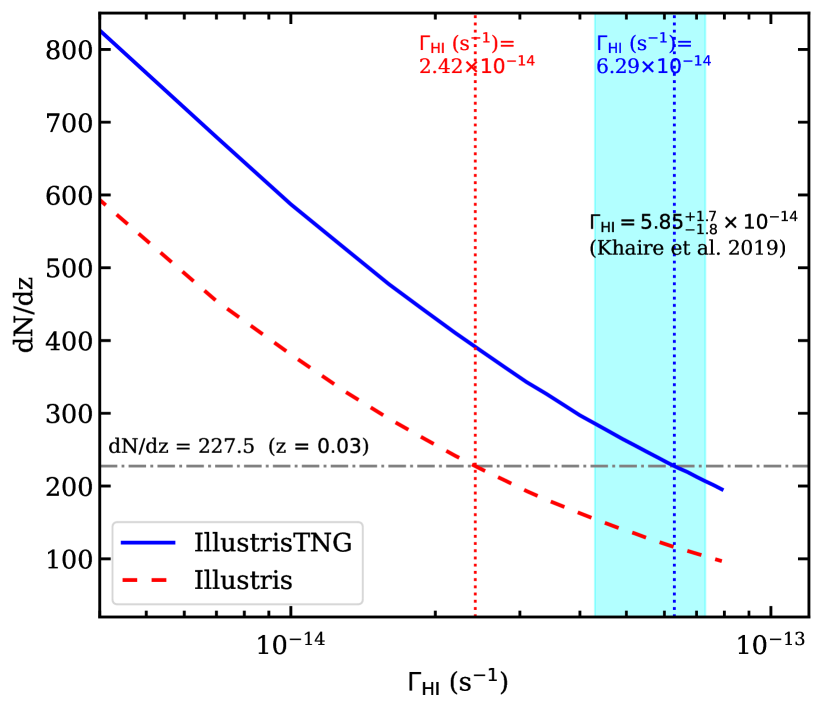
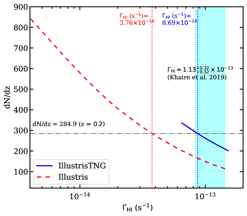
Figure 11: The line density ${\rm dN/dz}$ for Ly$\alpha$ absorbers in the range $10^{12}<N_{\rm HI}<10^{14.5}\,{\rm cm^{-2}}$ is plotted for IllustrisTNG (blue curve) and Illustris (red dashed curve) simulations at $z=0.03$ (left) and $z=0.2$ (right) using forward-modeled spectra. The grey dot-dashed line shows ${\rm dN/dz}$, obtained by fitting Voigt profiles to the Ly$\alpha$ forest observed in HST COS data from Danforth et al. (2016) in the redshift bins $0.005<z<0.06$ (left-hand panel) and $0.16<z<0.26$ (right-hand panel). The vertical dotted lines indicate the values of $\Gamma_{\rm HI}$ for Illustris (red) and IllustrisTNG (blue) at which the simulations match the ${\rm dN/dz}$ of the data. The cyan-shaded region shows the measurements of $\Gamma_{\rm HI}$ and its 1$\sigma$ uncertainty obtained by Khaire et al. (2019).

References

- Adams et al. (2011) Adams J. J., Uson J. M., Hill G. J., MacQueen P. J., 2011, ApJ, 728, 107
- Almgren et al. (2013) Almgren A. S., Bell J. B., Lijewski M. J., Lukić Z., Van Andel E., 2013, ApJ, 765, 39
- Bajtlik et al. (1988) Bajtlik S., Duncan R. C., Ostriker J. P., 1988, ApJ, 327, 570
- Bode et al. (2000) Bode P., Ostriker J. P., Xu G., 2000, ApJS, 128, 561
- Boera et al. (2019) Boera E., Becker G. D., Bolton J. S., Nasir F., 2019, ApJ, 872, 101
- Bolton et al. (2022a) Bolton J. S., Caputo A., Liu H., Viel M., 2022a, arXiv e-prints, p. arXiv:2206.13520
- Bolton et al. (2022b) Bolton J. S., Gaikwad P., Haehnelt M. G., Kim T.-S., Nasir F., Puchwein E., Viel M., Wakker B. P., 2022b, MNRAS, 513, 864
- Bower et al. (2006) Bower R. G., Benson A. J., Malbon R., Helly J. C., Frenk C. S., Baugh C. M., Cole S., Lacey C. G., 2006, MNRAS, 370, 645
- Burchett et al. (2019) Burchett J. N., et al., 2019, ApJ, 877, L20
- Burkhart et al. (2022) Burkhart B., Tillman M., Gurvich A. B., Bird S., Tonnesen S., Bryan G. L., Hernquist L., Somerville R. S., 2022, ApJ, 933, L46
- Carswell & Webb (2014) Carswell R. F., Webb J. K., 2014, VPFIT: Voigt profile fitting program (ascl:1408.015)
- Cen & Ostriker (1999) Cen R., Ostriker J. P., 1999, ApJ, 514, 1
- Cen & Ostriker (2006) Cen R., Ostriker J. P., 2006, ApJ, 650, 560
- Chabanier et al. (2020) Chabanier S., Bournaud F., Dubois Y., Palanque-Delabrouille N., Yèche C., Armengaud E., Peirani S., 2020, arXiv e-prints, p. arXiv:2002.02822
- Christiansen et al. (2019) Christiansen J. F., Davé R., Sorini D., Anglés-Alcázar D., 2019, arXiv e-prints, p. arXiv:1911.01343
- Croton et al. (2006) Croton D. J., et al., 2006, MNRAS, 365, 11
- Danforth et al. (2016) Danforth C. W., et al., 2016, ApJ, 817, 111
- Davé & Tripp (2001) Davé R., Tripp T. M., 2001, ApJ, 553, 528
- Davé et al. (2001) Davé R., et al., 2001, ApJ, 552, 473
- Davé et al. (2010) Davé R., Oppenheimer B. D., Katz N., Kollmeier J. A., Weinberg D. H., 2010, MNRAS, 408, 2051
- Davé et al. (2019) Davé R., Anglés-Alcázar D., Narayanan D., Li Q., Rafieferantsoa M. H., Appleby S., 2019, MNRAS, 486, 2827
- Debuhr et al. (2011) Debuhr J., Quataert E., Ma C.-P., 2011, MNRAS, 412, 1341
- Dove & Shull (1994) Dove J. B., Shull J. M., 1994, ApJ, 423, 196
- Dubois et al. (2014) Dubois Y., et al., 2014, MNRAS, 444, 1453
- Eckert et al. (2015) Eckert D., et al., 2015, Nature, 528, 105
- Faucher-Giguère et al. (2009) Faucher-Giguère C.-A., Lidz A., Zaldarriaga M., Hernquist L., 2009, ApJ, 703, 1416
- Fukugita et al. (1998) Fukugita M., Hogan C. J., Peebles P. J. E., 1998, ApJ, 503, 518
- Fumagalli et al. (2017) Fumagalli M., Haardt F., Theuns T., Morris S. L., Cantalupo S., Madau P., Fossati M., 2017, MNRAS, 467, 4802
- Gaikwad et al. (2017a) Gaikwad P., Khaire V., Choudhury T. R., Srianand R., 2017a, MNRAS, 466, 838
- Gaikwad et al. (2017b) Gaikwad P., Srianand R., Choudhury T. R., Khaire V., 2017b, MNRAS, 467, 3172
- Gaikwad et al. (2021) Gaikwad P., Srianand R., Haehnelt M. G., Choudhury T. R., 2021, MNRAS, 506, 4389
- Genel et al. (2014) Genel S., et al., 2014, MNRAS, 445, 175
- Genel et al. (2018) Genel S., et al., 2018, MNRAS, 474, 3976
- Gurvich et al. (2017) Gurvich A., Burkhart B., Bird S., 2017, ApJ, 835, 175
- Haardt & Madau (2012) Haardt F., Madau P., 2012, ApJ, 746, 125
- Hiss et al. (2018) Hiss H., Walther M., Hennawi J. F., Oñorbe J., O’Meara J. M., Rorai A., Lukić Z., 2018, ApJ, 865, 42
- Hiss et al. (2019) Hiss H., Walther M., Oñorbe J., Hennawi J. F., 2019, ApJ, 876, 71
- Hopkins et al. (2008) Hopkins P. F., Hernquist L., Cox T. J., Kereš D., 2008, ApJS, 175, 356
- Hu et al. (2022) Hu T., et al., 2022, MNRAS, 515, 2188
- Hu et al. (2023) Hu T., Khaire V., Hennawi J. F., Onorbe J., Walther M., Lukic Z., Davies F., 2023, arXiv e-prints, p. arXiv:2308.14738
- Hui & Gnedin (1997) Hui L., Gnedin N. Y., 1997, MNRAS, 292, 27
- Hussain et al. (2017) Hussain T., Khaire V., Srianand R., Muzahid S., Pathak A., 2017, MNRAS, 466, 3133
- Irsic et al. (2017) Irsic V., et al., 2017, Physical Review D, 96, 023522
- Johnson et al. (2019) Johnson S. D., et al., 2019, ApJ, 884, L31
- Khaire (2017) Khaire V., 2017, MNRAS, 471, 255
- Khaire & Srianand (2015) Khaire V., Srianand R., 2015, MNRAS, 451, L30
- Khaire & Srianand (2019) Khaire V., Srianand R., 2019, MNRAS, 484, 4174
- Khaire et al. (2016) Khaire V., Srianand R., Choudhury T. R., Gaikwad P., 2016, MNRAS, 457, 4051
- Khaire et al. (2019) Khaire V., et al., 2019, MNRAS, 486, 769
- Khaire et al. (2023) Khaire V., Hu T., Hennawi J. F., Burchett J. N., Walther M., Davies F., 2023, arXiv e-prints, p. arXiv:2311.08470
- Kollmeier et al. (2006) Kollmeier J. A., Miralda-Escudé J., Cen R., Ostriker J. P., 2006, ApJ, 638, 52
- Kollmeier et al. (2014) Kollmeier J. A., et al., 2014, ApJ, 789, L32
- Le Brun et al. (2014) Le Brun A. M. C., McCarthy I. G., Schaye J., Ponman T. J., 2014, MNRAS, 441, 1270
- Lee et al. (2015) Lee K.-G., et al., 2015, ApJ, 799, 196
- Lehner et al. (2007) Lehner N., Savage B. D., Richter P., Sembach K. R., Tripp T. M., Wakker B. P., 2007, ApJ, 658, 680
- Lomb (1976) Lomb N. R., 1976, Ap&SS, 39, 447
- Lukić et al. (2015) Lukić Z., Stark C. W., Nugent P., White M., Meiksin A. A., Almgren A., 2015, MNRAS, 446, 3697
- Maitra et al. (2022) Maitra S., Srianand R., Gaikwad P., Khandai N., 2022, MNRAS, 509, 4585
- Mallik & Srianand (2023) Mallik S., Srianand R., 2023, arXiv e-prints, p. arXiv:2309.05717
- Mallik et al. (2023) Mallik S., Srianand R., Maitra S., Gaikwad P., Khandai N., 2023, MNRAS, 523, 2296
- Martizzi et al. (2019) Martizzi D., et al., 2019, MNRAS, 486, 3766
- McDonald et al. (2006) McDonald P., et al., 2006, ApJS, 163, 80
- McQuinn & Upton Sanderbeck (2016) McQuinn M., Upton Sanderbeck P. R., 2016, MNRAS, 456, 47
- McQuinn et al. (2009) McQuinn M., Lidz A., Zaldarriaga M., Hernquist L., Hopkins P. F., Dutta S., Faucher-Giguère C.-A., 2009, ApJ, 694, 842
- Naiman et al. (2018) Naiman J. P., et al., 2018, MNRAS, 477, 1206
- Narayanan et al. (2012) Narayanan A., Savage B. D., Wakker B. P., 2012, ApJ, 752, 65
- Nasir et al. (2017) Nasir F., Bolton J. S., Viel M., Kim T.-S., Haehnelt M. G., Puchwein E., Sijacki D., 2017, MNRAS, 471, 1056
- Nelson et al. (2018a) Nelson D., et al., 2018a, MNRAS, 475, 624
- Nelson et al. (2018b) Nelson D., et al., 2018b, MNRAS, 475, 624
- Nelson et al. (2019) Nelson D., et al., 2019, MNRAS, 490, 3234
- Nicastro et al. (2018) Nicastro F., et al., 2018, Nature, 558, 406
- Persic & Salucci (1992) Persic M., Salucci P., 1992, MNRAS, 258, 14P
- Pillepich et al. (2018a) Pillepich A., et al., 2018a, MNRAS, 473, 4077
- Pillepich et al. (2018b) Pillepich A., et al., 2018b, MNRAS, 475, 648
- Pillepich et al. (2019) Pillepich A., et al., 2019, MNRAS, 490, 3196
- Planck Collaboration et al. (2018) Planck Collaboration et al., 2018, preprint, (arXiv:1807.06209)
- Prochaska et al. (2009) Prochaska J. X., Worseck G., O’Meara J. M., 2009, ApJ, 705, L113
- Rahmati et al. (2013) Rahmati A., Pawlik A. H., Raicevic M., Schaye J., 2013, MNRAS, 430, 2427
- Savage et al. (2011) Savage B. D., Narayanan A., Lehner N., Wakker B. P., 2011, ApJ, 731, 14
- Savage et al. (2014) Savage B. D., Kim T.-S., Wakker B. P., Keeney B., Shull J. M., Stocke J. T., Green J. C., 2014, ApJS, 212, 8
- Scargle (1982) Scargle J. D., 1982, ApJ, 263, 835
- Schaye et al. (2015) Schaye J., et al., 2015, MNRAS, 446, 521
- Shull et al. (2010) Shull J. M., France K., Danforth C. W., Smith B., Tumlinson J., 2010, ApJ, 722, 1312
- Shull et al. (2012) Shull J. M., Smith B. D., Danforth C. W., 2012, ApJ, 759, 23
- Shull et al. (2015) Shull J. M., Moloney J., Danforth C. W., Tilton E. M., 2015, ApJ, 811, 3
- Sijacki et al. (2007) Sijacki D., Springel V., Di Matteo T., Hernquist L., 2007, MNRAS, 380, 877
- Springel (2005) Springel V., 2005, MNRAS, 364, 1105
- Springel (2010) Springel V., 2010, MNRAS, 401, 791
- Tanimura et al. (2019) Tanimura H., et al., 2019, MNRAS, 483, 223
- Tejos et al. (2016) Tejos N., et al., 2016, MNRAS, 455, 2662
- Tepper-García (2006) Tepper-García T., 2006, MNRAS, 369, 2025
- Tepper-García et al. (2012) Tepper-García T., Richter P., Schaye J., Booth C. M., Dalla Vecchia C., Theuns T., 2012, MNRAS, 425, 1640
- Theuns et al. (2000) Theuns T., Schaye J., Haehnelt M. G., 2000, MNRAS, 315, 600
- Theuns et al. (2002) Theuns T., Viel M., Kay S., Schaye J., Carswell R. F., Tzanavaris P., 2002, ApJ, 578, L5
- Tillman et al. (2022) Tillman M. T., Burkhart B., Tonnesen S., Bird S., Bryan G. L., Anglés-Alcázar D., Davé R., Genel S., 2022, arXiv e-prints, p. arXiv:2210.02467
- Tornatore et al. (2010) Tornatore L., Borgani S., Viel M., Springel V., 2010, MNRAS, 402, 1911
- Tripp et al. (2008) Tripp T. M., Sembach K. R., Bowen D. V., Savage B. D., Jenkins E. B., Lehner N., Richter P., 2008, ApJS, 177, 39
- Tuominen et al. (2021) Tuominen T., et al., 2021, A&A, 646, A156
- Viel & Haehnelt (2006) Viel M., Haehnelt M. G., 2006, MNRAS, 365, 231
- Viel et al. (2013a) Viel M., Becker G. D., Bolton J. S., Haehnelt M. G., 2013a, Phys. Rev. D, 88, 043502
- Viel et al. (2013b) Viel M., Schaye J., Booth C. M., 2013b, MNRAS, 429, 1734
- Viel et al. (2017) Viel M., Haehnelt M. G., Bolton J. S., Kim T.-S., Puchwein E., Nasir F., Wakker B. P., 2017, MNRAS, 467, L86
- Vogelsberger et al. (2014) Vogelsberger M., et al., 2014, MNRAS, 444, 1518
- Walther et al. (2018) Walther M., Hennawi J. F., Hiss H., Oñorbe J., Lee K.-G., Rorai A., 2018, ApJ, 852, 22
- Walther et al. (2019) Walther M., Oñorbe J., Hennawi J. F., Lukić Z., 2019, ApJ, 872, 13
- Weinberg et al. (1997) Weinberg D. H., Hernquist L., Katz N., 1997, ApJ, 477, 8
- Weinberger et al. (2017) Weinberger R., et al., 2017, MNRAS, 465, 3291
- Werk et al. (2016) Werk J. K., et al., 2016, ApJ, 833, 54
- Worseck et al. (2011) Worseck G., et al., 2011, ApJ, 733, L24
- Yèche et al. (2017) Yèche C., Palanque-Delabrouille N., Baur J., du Mas des Bourboux H., 2017, J. Cosmology Astropart. Phys., 6, 047
- de Graaff et al. (2019) de Graaff A., Cai Y.-C., Heymans C., Peacock J. A., 2019, A&A, 624, A48