Exchange–correlation bound states of the triplet soft–sphere fermions by the path integral Monte Carlo simulations

Abstract

Path integral Monte Carlo simulations in the Wigner approach to quantum mechanics has been applied to calculate momentum and spin–resolved radial distribution functions of the strongly correlated soft–sphere quantum fermions. The obtained spin–resolved radial distribution functions demonstrate arising triplet clusters of fermions, that is the consequence of the interference of exchange and interparticle interactions. The semiclassical analysis in the framework of the Bohr–Sommerfeld quantization condition applied to the potential of the mean force corresponding to the same–spin radial distribution functions allows to detect exchange–correlation bound states in triplet clusters and to estimate corresponding averaged energy levels. The obtained momentum distribution functions demonstrate the narrow sharp separated peaks corresponding to bound states and disturbing the Maxwellian distribution.

I Introduction

There are a number of simple model pair potentials for a strongly coupled system of particles, which are useful in statistical mechanics and capable of grasping some physical properties of complex systems. The examples include the soft- and hard-sphere fluids as well as the Lennard-Jones system. The one component plasma is of great astrophysical importance being an excellent model for describing many features of superdense, completely ionized matter typical for white dwarfs, the outer layers of neutron stars and possibly the interiors of heavy planets Luyten (1971); Potekhin (2010). Properties and structure of strongly correlated bosonic systems of hard- and soft-spheres are systematically studied in the literature using different many-body approaches Boronat et al. (2000); Mazzanti et al. (2003); Sesé (2020); Nozieres and Pines (2018). In such systems maxima in radial and momentum distribution functions and the excitation spectrum are observed, which is a natural effect of the correlations when density increases. The quantum interparticle correlations in triplets of particles are difficult to investigate while the triplet correlations are important for any statistical analysis Sesé (2020), as they allow to formulate thermodynamic properties beyond the pairwise approach.

On the other hand, the theoretical studies of the strongly interacting particles obeying the Fermi–Dirac statistics is a subject of general interest in many fields of physics. This work deals with the physical properties of a model system composed of strongly interacting soft-sphere fermions at non-zero temperatures. In the case of strong interparticle interaction perturbative methods cannot be applied, so direct computer simulations have to be used. At finite temperatures the most widespread numerical method in quantum statistics is a Monte–Carlo (MC) method usually based on the representation of the quantum partition function in the form of path integrals in the coordinate space of particles Feynman and Hibbs (1965); Zamalin et al. (1977). A direct computer simulation allows one to calculate a number of properties provided that the interaction potential is known. For example, a path integral Monte-Carlo (PIMC) method is used to study thermodynamic properties of dense noble gases, dense hydrogen, electron-hole and quark-gluon plasmas, etc. Ebeling et al. (2017); Fortov et al. (2020); Dornheim et al. (2018); Ceperley (1995); Pollock and Ceperley (1984); Singer and Smith (1988); Filinov et al. (2022a).

In this article we are going to use the PIMC method to study the properties of strongly correlated soft–sphere fermions. However the main difficulty of the PIMC method for Fermi systems is the “fermionic sign problem” arising due to the antisymmetrization of a fermion density matrix Feynman and Hibbs (1965) and resulting in thermodynamic quantities to be small differences of large numbers associated with even and odd permutations. As a consequence, the statistical error in PIMC simulations grows exponentially with the number of particles. To overcome this issue a lot of approaches have been developed. In Ceperley (1991, 1992) to avoid the “fermionic sign problem”, a restricted fixed–node path–integral Monte Carlo (RPIMC ) approach has been developed. In RPIMC only positive permutations are taken into account, so the accuracy of the results is unknown. More consistent approaches are the permutation blocking path integral Monte Carlo (PB-PIMC) and the configuration path integral Monte Carlo (CPIMC) methods Dornheim et al. (2018). In CPIMC the density matrix is presented as a path integral in the space of occupation numbers. However it turns out that both methods also exhibit the “sign problem” worsening the accuracy of PIMC simulations.

An alternative approach based on the Wigner formulation of quantum mechanics in the phase space Wigner (1934); Tatarskii (1983) was used in Larkin et al. (2017a, b) to avoid the antisymmetrization of matrix elements and hence the “sign problem”. This approach allows to realize the Pauli blocking of fermions and is able to calculate quantum momentum distribution functions as well as transport properties Ebeling et al. (2017); Fortov et al. (2020).

We use the modified path integral representation of the Wigner function and the MC approach (WPIMC) to calculate the radial and momentum distribution functions of a soft–sphere fermionic system. The WPIMC allows also to reduce the “sign problem” in contrast to a standard PIMC. To overcome the “sign problem” the exchange interaction is expressed through a positive semidefinite Gram determinant Filinov et al. (2021) in the expression for the density matrix. This article is the continuation of our publications on the improvements of the PIMC approach for strongly correlated systems of fermions and degenerate plasma media Zamalin et al. (1977); Ebeling et al. (2017); Fortov et al. (2020); Filinov et al. (2015, 2020, 2021); Filinov et al. (2022b).

We consider a 3D system of $N$ soft–spheres obeying the Fermi–Dirac statistics in the canonical ensemble at a finite temperature. In our approach the fermions interact through a quantum pseudopotential corresponding to the soft–sphere potential $\phi(x)=\epsilon(\sigma/x)^{n}$, where $x$ is the interparticle distance, $\sigma$ characterizes the effective particle size, $\epsilon$ sets the energy scale and $n$ is a parameter determining the potential hardness. The density of soft spheres is characterized by the parameter $r_{s}=a/\sigma$, defined as the ratio of the mean distance between the particles $a=\left[3/(4\pi\tilde{\rho})\right]^{1/3}$ to $\sigma$ ($\tilde{\rho}$ is the number density). For example, the results presented below have been obtained for the following physical parameters used in Filinov et al. (2022a) for PIMC simulations of helium-3: $\epsilon=26.7{\rm K}$, $\sigma=5.19\,a_{\rm B}$ ($a_{\rm B}$ is the Bohr radius), $m_{a}=3.016$ is the soft–sphere mass in atomic units. Other parameters are: $T=60\,{\rm K}$, $r_{s}\approx 0.844$, so that $\lambda/\sigma\approx 0.48$, where $\lambda=\sqrt{2\pi\hbar^{2}\beta/m}$ is the thermal wavelength of a fermion, $\beta=1/(k_{B}T)$ is the inverse temperature, $m$ is the mass of a fermion.

In section II we consider the path integral description of quantum soft–sphere fermions. In section III we derive a pseudopotential for the soft spheres accounting for the quantum effects in the interparticle interaction. In section IV we present the results of our simulations. The momentum distribution functions of the strongly coupled soft–sphere fermions calculated by WPIMC for different $n$ are discussed in subsection IV.A. Subsection IV.B deals with WPIMC spin–resolved radial distribution functions demonstrating the short–range ordering of fermions (triplet fermion clusters) caused by the interference of the exchange and interparticle interactions. In subsection IV.C the exchange–correlation bound states of fermion triplets and corresponding averaged energy levels have been obtained from the Bohr–Sommerfeld quantization condition applied to the potential of the mean force corresponding to the same–spin radial distribution functions. In section V we summarize the basic results and discuss their physical meaning.

II Path integral representation of Wigner function

Let us consider $N$ quantum soft–sphere fermions. The Hamiltonian of the system ${\hat{H}}={\hat{K}}+{\hat{U}}$ contains kinetic energy ${\hat{K}}$ and interaction energy ${\hat{U}}$ contributions taken as the sum of pair interactions $\phi(x)$. Since the operators of kinetic and potential energy do not commutate, the exact explicit analytical expression for the Wigner function is unknown but can be formally constructed using a path integral approach Feynman and Hibbs (1965); Zamalin and Norman (1973); Zamalin et al. (1977) based on the operator identity $e^{-\beta{\hat{H}}}=e^{-\epsilon{\hat{H}}}\cdot e^{-\epsilon{\hat{H}}}\dots e^{-\epsilon{\hat{H}}}$, where $\epsilon=\beta/M$ and $M$ is a positive integer number. The Wigner function of the multiparticle system in the canonical ensemble is defined as the Fourier transform of the off–diagonal matrix element of the density matrix in the coordinate representation Wigner (1934); Tatarskii (1983); Feynman and Hibbs (1965); Fortov et al. (2020); Zamalin et al. (1977); Larkin and Filinov (2017); Larkin et al. (2016); Wiener (1923); Zamalin and Norman (1973). The antisymmetrized Wigner function can be written in the form:

$$W(p,x;\beta)=\frac{1}{Z(N,V;\beta)N!\lambda^{3N}}\sum_{\sigma}\sum_{P}(-1)^{\kappa_{P}}{\cal S}(\sigma,{\hat{P}}\sigma^{\prime})\big{|}_{\sigma^{\prime}=\sigma}\,\int{\rm d}\xi e^{i\langle\xi|p\rangle/\hbar}\langle x-\xi/2|e^{-\beta\hat{H}}|x+\xi/2\rangle\\ \approx\frac{1}{Z(\beta)N!\lambda^{3N}}\sum_{\sigma}\sum_{P}(-1)^{\kappa_{P}}{\cal S}(\sigma,{\hat{P}}\sigma^{\prime})\big{|}_{\sigma^{\prime}=\sigma}\,\int{\rm d}\xi e^{i\langle\xi|p\rangle/\hbar}\langle x-\xi/2|\prod_{m=0}^{M-1}e^{-\epsilon{\hat{U}_{m}}}e^{-\epsilon{\hat{K}_{m}}}|{\hat{P}}(x+\xi/2)\rangle.$$ (1)

The partition function $Z$ for a given temperature $T$ and fixed volume $V$ is defined by the expression:

$$Z(N,V;\beta)=\frac{1}{N!\lambda^{3N}}\sum_{\sigma}\int\limits_{V}{\rm d}x\,\rho(x,\sigma;\beta),$$ (2)

where $\rho(x,\sigma;\beta)$ denotes the diagonal matrix elements of the density operator ${\hat{\rho}}=e^{-\beta{\hat{H}}}$. Here $x$ and $\sigma$ are vector variables of the spatial coordinates and spin degrees of freedom of particles, $\lambda=\sqrt{\frac{2\pi\hbar^{2}\beta}{m}}$ is the thermal wavelength. The integral in Eq. (2) can be rewritten as:

$$\sum_{\sigma}\int\limits{\rm d}x^{(0)}\,\rho(x^{(0)},\sigma;\beta)=\int\limits{\rm d}x^{(0)}\dots\rm dx^{(M-1)}\,\rho^{(1)}\dots\rho^{(M-1)}\sum_{\sigma}\sum_{P_{e}}(-1)^{\kappa_{P}}\,{\cal S}(\sigma,{\hat{P}}\sigma^{\prime})\,{\hat{P}}\rho^{(M)}\big{|}_{x^{(M)}=x^{(0)},\sigma^{\prime}=\sigma}\,\\ \approx{}\int{{\rm d}x^{(0)}\dots\rm dx^{(M-1)}}\exp\Biggl{\{}-\sum_{m=0}^{M-1}\biggl{[}\pi\left|x^{(m)}-x^{(m+1)}\right|^{2}+\epsilon U(x^{(m)})\biggr{]}\Biggr{\}}{\rm det}\|\Psi(x)\|,$$ (3)

where we imply that momentum and coordinate are dimensionless variables $p\tilde{\lambda}/\hbar$ and $x/\tilde{\lambda}$ related to a temperature $\sim 1/\epsilon$ ($\tilde{\lambda}=\sqrt{2\pi\hbar\beta/(mM)}$). Spin gives rise to the standard spin part of the density matrix ${\cal S}(\sigma,{\hat{P}}\sigma^{\prime})=\prod_{k=1}^{N}\delta(\sigma_{k},\sigma_{Pk})$, ($\delta(\sigma_{k},\sigma_{t})$ is the Kronecker symbol) with exchange effects accounted for by the permutation operator $\hat{P}$ acting on coordinates of particles $x^{(M)}$ and spin projections $\sigma^{\prime}$. The sum is taken over all permutations with a parity $\kappa_{P}$. In Eqs. (1), (3) index $m=0,\dots,M-1$ labels the off–diagonal high–temperature density matrices $\rho^{(m)}\equiv\rho\left(x^{(m)},x^{(m+1)};\epsilon\right)=\langle x^{(m)}|e^{-\epsilon{\hat{H}}}|x^{(m+1)}\rangle$. With the error of the order of $1/M^{2}$ each high–temperature factor can be presented in the form $\langle x^{(m)}|e^{-\epsilon{\hat{H}}}|x^{(m+1)}\rangle\approx\langle x^{(m)}|e^{-\epsilon{\hat{U}}}|x^{(m+1)}\rangle\rho^{(m)}_{0}$ with $\rho^{(m)}_{0}=\langle x^{(m)}|e^{-\epsilon{\hat{K}}}|x^{(m+1)}\rangle$, arising from neglecting the commutator $\epsilon^{2}\left[K,U\right]/2$ and higher powers of $\epsilon$ terms. In the limit $M\rightarrow\infty$ the error of the whole product of high temperature factors is equal to zero $(\propto 1/M)$ and we have an exact path integral representation of the Wigner and partition functions, in which each particle is represented by a trajectory consisting of a set of $M$ coordinates (“beads”): $\tilde{x}\equiv\{x_{1}^{(0)},\dots x_{1}^{(M-1)},x_{2}^{(0)}\ldots x_{2}^{(M-1)},\ldots x_{N}^{(M-1)}$. In the thermodynamic limit the main contribution in the sum over spin variables comes from the term related to the equal numbers ($N/2$) of fermions with the same spin projection Ebeling et al. (2017); Fortov et al. (2020). The sum over permutations gives the product of determinants: $\mathrm{det}\|\Psi(x)\|=\mathrm{det}\bigl{\|}e^{-{\pi}\left|x_{k}^{(M)}-x_{t}^{(0)}\right|^{2}}\bigr{\|}_{1}^{N/2}\mathrm{det}\bigl{\|}e^{-{\pi}\left|x_{k}^{(M)}-x_{t}^{(0)}\right|^{2}}\bigr{\|}_{(N/2+1)}^{N}$.

In general the complex-valued integral over $\xi$ in the definition of the Wigner function (1) can not be calculated analytically and is inconvenient for Monte Carlo simulations. The second disadvantage is that Eqs. (1), (3) contain the sign–altering determinant ${\rm det}\|\Psi(x)\|$, which is the reason of the “sign problem” worsening the accuracy of PIMC simulations. To overcome these problems let us replace the variables of integration $x^{(m)}$ by $q^{(m)}$ for any given permutation $P$ using the substitution Larkin et al. (2016, 2017b):

$$x^{(m)}=(Px-x)\frac{m}{M}+x+q^{(m)}\\ {}-\frac{(M-m)\xi}{2M}+\frac{mP\xi}{2M},$$ (4)

where $P$ is the matrix representing a permutation and equal to the unit matrix $E$ with appropriately transposed columns. This replacement presents each trajectory as a sum of the “straight line” ($(Px-x)\frac{m}{M}+x-\frac{(M-m)\xi}{2M}+\frac{mP\xi}{2M}$) and the deviation from it ($q^{(m)}$). As a consequence the matrix elements of the density matrix can be rewritten in the form of a path integral over “closed” trajectories $\{q^{(0)},\dots,q^{(M)}\}$ with $q^{(0)}=q^{(M)}=0$ and after the integration over $\xi$ Larkin et al. (2016, 2017b) and some additional transformations (see Filinov et al. (2020, 2021) for details) the Wigner function can be written in the form containing the Maxwell distribution with quantum corrections:

$$W(p,x;\beta)\approx\frac{\tilde{C}(M)}{Z(\beta)N!}\int{\rm d}q^{(1)}\dots\rm dq^{(M-1)}\exp\Bigl{[}-\sum\limits_{m=0}^{M-1}\biggl{(}\pi|\eta^{(m)}|^{2}-\epsilon U\biggl{(}x+q^{(m)}\biggr{)}\biggr{)}\Bigr{]}\\ \times\exp\Biggl{\{}\frac{M}{4\pi}\left<ip-\frac{\epsilon}{2}\sum\limits_{m=0}^{M-1}\frac{(M-2m)}{M}\frac{\partial U(x+q^{(m)})}{\partial x}\Bigg{|}ip-\frac{\epsilon}{2}\sum\limits_{m=0}^{M-1}\frac{(M-2m)}{M}\frac{\partial U(x+q^{(m)})}{\partial x}\right>\Biggr{\}}\\ \times\mathrm{det}\|\tilde{\phi}_{kt}\bigl{\|}_{1}^{N/2}\mathrm{det}\bigr{\|}\tilde{\phi}_{kt}\|_{(N/2+1)}^{N_{e}},\,$$ (5)

where

$$\tilde{\phi}_{kt}=\exp\{-{\pi}\left|r_{kt}\right|^{2}/M\}\exp\Biggl{\{}-\frac{1}{2}\sum\limits_{m=0}^{M-1}\biggl{(}\epsilon\phi\Bigl{(}\Bigl{|}r_{tk}\frac{2m}{M}+r_{kt}+q_{kt}^{(m)}\Bigr{|}\Bigr{)}-{}\epsilon\phi\Bigl{(}\Bigl{|}r_{kt}+q_{kt}^{(m)}\Bigr{|}\Bigr{)}\biggr{)}\Biggr{\}},$$

and $i$ is imaginary unit, $\eta^{(m)}\equiv q^{(m)}-q^{(m+1)}$, $r_{kt}\equiv(x_{k}-x_{t})$, $(k,t=1,\dots,N)$. The constant $\tilde{C}(M)$ is canceled in Monte Carlo calculations.

Let us stress that the approximate implementation of the Wigner function used in our simulations and specified in Eq. (5) accounts for the contribution of all permutations in the form of the determinants $\mathrm{det}\|\tilde{\phi}_{kt}\bigl{\|}_{1}^{N/2}\mathrm{det}\bigr{\|}\tilde{\phi}_{kt}\|_{(N/2+1)}^{N_{e}}$. Moreover, approximation (5) have the correct limits to the cases of weakly and strongly degenerate fermionic systems. Indeed, in the classical limit the main contribution comes from the diagonal matrix elements due to the factor $\exp\{-{\pi}\left|r_{kt}\right|^{2}/M\}$ and the differences of potential energies in the exponents are equal to zero (identical permutation). At the same time, when the thermal wavelength is of the order of the average interparticle distance and the trajectories are highly entangled the term $r_{tk}\frac{2m}{M}$ in the potential energy $\phi\Bigl{(}\Bigl{|}r_{tk}\frac{2m}{M}+r_{kt}+q_{kt}^{(m)}\Bigr{|}\Bigr{)}$ can be omitted and the differences of potential energies in the exponents tend to zero Filinov et al. (2020, 2021).

III Quantum pseudopotential for soft–sphere fermions

As alternative the high–temperature density matrix $\rho^{(m)}=\langle x^{(m)}|e^{-\epsilon{\hat{H}}}|x^{(m+1)}\rangle$ can be expressed as a product of two–particle density matrices Ebeling et al. (2017)

$$\rho(x_{l},x^{\prime}_{l},x_{t},x^{\prime}_{t};\epsilon)=\frac{1}{\tilde{\lambda}^{6}}\exp\left[-\frac{\pi}{\tilde{\lambda}^{2}}|x_{l}-x^{\prime}_{l}|^{2}\right]\\ {}\times\exp\left[-\frac{\pi}{\tilde{\lambda}^{2}}|x_{t}-x^{\prime}_{t}|^{2}\right]\exp[-\epsilon\Phi^{OD}_{lt}]\,.$$ (6)

This formula results from the factorization of the density matrix into the kinetic and potential parts, $\rho\approx\rho_{0}^{K}\rho^{U}$. The off–diagonal density matrix element (6) involves an effective pair interaction by a pseudopotential, which can be expressed approximately via its diagonal elements, $\Phi^{OD}_{lt}(x_{l},x^{\prime}_{l},x_{t},x^{\prime}_{t};\epsilon)\approx[\Phi_{lt}(x_{l}-x_{t};\epsilon)+\Phi_{lt}(x^{\prime}_{l}-x^{\prime}_{t};\epsilon)]/2$. To estimate $\Phi(x)$ for each high temperature density matrix we use the well known semiclassical approximation Feynman and Hibbs (1965):

$$\epsilon\Phi(x;\epsilon)=\left(\frac{12}{{\tilde{\lambda}}_{r}^{2}}\right)^{3/2}\,\int\limits_{-\infty}^{+\infty}\epsilon\phi(y+x)\exp\left[{-\frac{12\pi y^{2}}{\tilde{\lambda}_{r}^{2}}}\right]{\rm d^{3}}y,$$ (7)

where $\tilde{\lambda}_{r}=\sqrt{2\pi\hbar^{2}\epsilon/\tilde{m}}$, $\tilde{m}=m/2$ is the reduced mass of a fermion. Averaging of the potential $\phi$ according to Eq. (7) reduces the hardness of the soft–sphere potential. As an illustration, Fig. 1 presents the bounded from above by the constant $h=10$ “hard–sphere” potential, its pseudopotential, the soft–sphere potential $\phi$ for $n=5/3$, the corresponding pseudopotentials $\Phi$ and its fitting soft–sphere approximation $\phi$ for $n\simeq 2/3$.

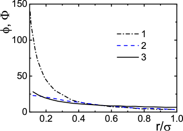
Figure 1: (Color online) Potentials $\phi$ (lines 1) and corresponding pseudopotentials $\Phi$ (lines 2) defined by Eq. (7) in conditional units. (Top panel) The bounded from above by the constant $h=10$ “hard–sphere” potential and the corresponding $\Phi$. (Bottom panel) The soft–sphere potential ($n=5/3$) and the corresponding $\Phi$ approximated by the soft–sphere $\phi$ with $n\sim 2/3$ (line 3)).

To derive a more accurate but more complicated pseudopotential $\Phi(x;\epsilon)$ for the potential $\phi(r)$ we have considered also the Kelbg functional Demyanov and Levashov (2022); Kelbg (1963) for the Fourier transform $v(t)$ of the potential $\phi(r)$. This transform can be found at $n<3$ for the corresponding Yukawa–like potential $exp(-\kappa r)/r^{n}$ in the limit of “zero screening” ($\kappa\rightarrow 0$:

$$v(t)=\frac{4\pi t^{n}\Gamma(2-n)\sin(n\pi/2)}{t^{3}}.$$ (8)

where $\Gamma$ is the gamma function. The resulting quantum pseudopotential has the following form:

$$\Phi(x,\epsilon)=\frac{\sqrt{\pi}}{8\pi^{3}}\times{}\\ \int^{\infty}_{0}v(t)\exp(-(\tilde{\lambda}t)^{2}/4)\frac{\sin(tr)\text{erfi}(\tilde{\lambda}t/2)}{(tr)\tilde{\lambda}t}4\pi t^{2}{\rm d}t,$$ (9)

where $\text{erfi}(z)=i\text{efr}(iz)$, $\text{efr}(z)$ is the error function, $r=|x|$ Demyanov and Levashov (2022). This pseudopotential is finite at zero distance and decreases according to the power law with increasing distance.

For more accurate accounting for quantum effects the “potential energy” $U(x^{(m)},x^{(m+1)})$ in (1) and (3) has to be taken as the sum of pair interactions given by $\Phi^{OD}$ with $\Phi(x;\epsilon)$. However, if the effective hardness of the pseudopotential $\Phi$ is less than $3$ the corresponding energy $\sum_{m=0}^{M-1}\epsilon U(x^{(m)})$ may be divergent in the thermodynamic limit. To overcome this deficiency let us modify the pseudopotential $\Phi$ according to the transformation considered in Hansen (1973):

$$\tilde{\Phi}(x;\epsilon)=\epsilon[\Phi(x;\epsilon)-\frac{1}{V}\int\limits_{V}{\rm d^{3}}y\Phi(x+y;\epsilon)]\\ {}=\epsilon\int\limits{\rm d^{3}}y\Phi(x+y;\epsilon)\left(\delta(y)-\frac{1}{V}\right).$$ (10)

Here the uniformly “charged” background is introduced to compensate the possible divergence of $U(x^{(m)})$ like in the one-component Coulomb plasma.

Systems of 100, 200 and 300 particles represented by twenty and forty “beads” interacting with the quantum pseudopotential $\tilde{\Phi}(x;\epsilon)$ given by approximations Eq. (7) as well as Eq. (10) have been considered in the basic Monte Carlo cell with periodic boundary conditions. The WPIMC configurations in the range of the $10^{6}-3\times 10^{6}$ of the Markovian chain have been generated to calculate distribution functions. So we have checked the convergence of the calculated distribution functions with increasing number of particles represented by the increasing number of beads in this range of parameters.

Let us note that the pseudopotential corresponding to the Coulomb potential with hardness $n=1$ was often used in PIMC simulations of one– and two–component plasma media in Kelbg (1963); Ebeling et al. (1967); Filinov et al. (2004); Ebeling et al. (2006); Klakow et al. (1994); Ebeling et al. (2017); Fortov et al. (2020) with good agreement with available in literature data. We used here the potentials with a hardness a bit more and less than unity. In the considered here range of hardnesses the convergence of the distribution functions was tested and it turns out that 300 particles represented by 20 beads is enough to reach the convergence.

IV Simulation results

In PIMC simulations some trajectories presenting fermions and starting in the basic Monte Carlo cell with periodic boundary conditions can “cross” a cell boundary. In this case the choice between the “basic cell bead” and its periodic image in the calculation of the interparticle interaction $U(x^{(m)},x^{(m+1)})$ becomes ambiguous that is discussed in detail in Ebeling et al. (2017); Fortov et al. (2020). Here this problem prevents making use of the Ewald technique for the calculation of the pseudopotential energy $U(x^{(m)},x^{(m+1)})$ in (1) and (3). The second problem is the slow decay of the pseudopotential $\tilde{\Phi}$.

Due to these problems we present only radial and momentum distribution functions, which demonstrate faster convergence with increasing number of particles in a Monte Carlo cell in comparison with thermodynamic quantities Filinov et al. (2020). The pair distribution function Kirkwood (1935); Fisher (1964) and momentum distribution function (MDF) can be written in the form:

$$g_{ab}(r)=\int\limits_{V}\frac{dpdx}{(2\pi)^{6N}}\,\delta(|x_{1,a}-x_{1,b}|-r)\,W(p,x;\beta),$$

$$w_{a}(|p|)=\int\limits_{V}\frac{dpdx}{(2\pi)^{6N}}\,\delta(|p_{1,a}|-|p|)\,W(p,x;\beta),$$ (11)

where $\delta$ is the delta function, $a$ and $b$ labels the spin value of the fermion. The pair distribution function $g_{ab}$ give the probability density to find a pair of particles of types $a$ and $b$ at a certain distance $r$ from each other and depends only on the difference of coordinates because of the translational invariance of the system. In a noninteracting classical system, $g_{ab}\equiv 1$, whereas interaction and quantum statistics result in a redistribution of the particles. The momentum distribution function $w_{a}(|p|)$ gives a probability density for particle of type $a$ to have a momentum $p$.

IV.1 Momentum distribution functions

Figure 2 presents the Maxwell momentum distribution function ($\sim\exp(-(p\lambda/\hbar)^{2}/4\pi$) (line $1$) and the WPIMC calculations of the momentum distribution functions (MDFs) for the potentials with $n=0.2$ (panel a)), $n=0.6$ (panel b)), $n=1.0$ (panel c)), $n=1.7$ (panel d)) for the mentioned above fixed density ($r_{s}\approx 0.844$) and temperature ($T=60\,{\rm K}$). All MDFs are normalized to unity. For a small hardness ($n=0.2$) of the pseudopotential as well as at large momentum the Maxwell distributions practically coincide with the WPIMC MDFs (all lines 2).

At the same time at a larger hardness ($n\geq 0.6$) and at smaller momentum lines 2 show the narrow separated peaks disturbing the Maxwell distribution. The physical meaning of these peaks as well as the circles $3$ and $4$ are discussed below.

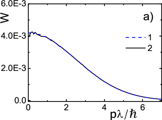
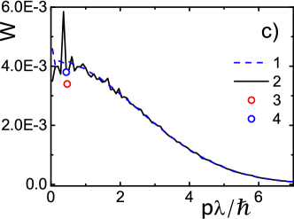
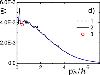
Figure 2: (Color online) WPIMC MDF $W(p\lambda/\hbar)$ for soft–sphere potentials with $n=0.2$—a); $n=0.6$—b); $n=1.0$—c); $n=1.4$—d). Lines: 1—the Maxwell MDF; 2—the WPIMC MDF for the same spin projections. Circles: 3, 4—momenta corresponding to the energy level with $n_{r}=0$ and $L=0$, $L=1$ (see below). Small irregular oscillations of the MDFs indicate Monte-Carlo statistical error.

The convergence and statistical error of distribution functions with increasing number of the steps in the Monte Carlo runs have been tested for increasing number of particles and number of beads at different softnesses of pseudopotentials. The width of the narrow sharp peaks in numerical distribution functions depends not only on the physical properties of the system but is also affected by the smallness of the discrete interval in the corresponding calculated histogram. With decreasing histogram interval the statistical errors increases due to worsening of statistics in each interval, so the compromise between reasonable value of discrete interval and the statistical errors have to be achieved. In our simulations the values of statistical errors are of the order of small random oscillations of the distribution functions, which are several times less than regular peaks.

IV.2 Radial distribution functions and the potential of mean force

To explain the existence and physical meaning of the individual separated sharp high peaks on the MDFs let us consider a typical random pseudopotential field created by $\Phi(x;\epsilon)$, radial distribution functions (RDF) and the corresponding potentials of mean interparticle force.

Fig. 3 shows a typical random pseudopotential field created by $\Phi(x;\epsilon)$ in a cross-section of the Monte Carlo cell. The vertical scale bar allows to estimate the pseudopotential field variation. As we shall see below from the consideration of RDFs and potentials of mean force the possible formation of cavities separated by barriers is the physical reason of arising bound states for a triplet of fermions.

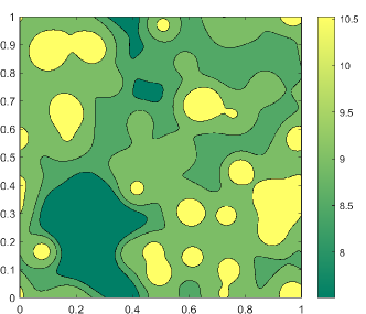
Figure 3: (Color online)Typical random pseudopotential field in a cross section of the Monte Carlo cell for the particles interacting with $\Phi(x;\epsilon)$ at $n=2/3$. The vertical scale bar demonstrates the pseudopotential field variation in arbitrary units.

The potential of mean force (PMF) $w^{(k)}$ Kirkwood (1935) of a classical $N$ particle system is defined up to an arbitrary constant as:

$$-\nabla_{j}w^{(k)}\,=\,{\frac{\int e^{-\beta U}(-\nabla_{j}U)dq_{k+1}\dots dq_{N}}{\int e^{-\beta U}dq_{k+1}\dots dq_{N}}},$$ (12)

where $j=1,2,\dots,k$. Above, $-\nabla_{j}w^{(k)}$ is the averaged force, i.e. the “mean force” acting on a particle $j$. For $k=2$ the $w^{(2)}$ is related to the RDF of the system as

$$g(r)=e^{{-\beta w^{{(2)}}(r)}}.$$ (13)

Let us note that an RDF can be expressed as a virial expansion which in the low-density limit is given by the formula Fisher (1964); Zelener et al. (1981):

$$g(r)=e^{-\beta\phi(r)}.$$ (14)

So the PMF $w^{{(2)}}(r)$ obtained from simulations determine to some extent the effective interparticle interaction and corresponding physical properties.

Figure 4 presents the results of our WPIMC calculations for the RDFs with the same and opposite spin projections for a fixed density and temperature but at different hardnesses of the soft–sphere pseudopotential. Let us discuss the difference revealed between the RDFs with the same and opposite spin projections. At small interparticle distances all RDFs tend to zero due to the repulsion nature of the soft–sphere potential. Additional contribution to the repulsion of fermions with the same spin projection at distances of the order of the thermal wavelength are caused by the Fermi statistics effect described by the exchange determinant in (5), which accounts for the interference effects of the exchange and interparticle interactions. This additional repulsion leads to the formation of cavities (usually called exchange–correlation holes) for fermions with the same spin projection and results in the formation of high peaks on the corresponding RDF due to the strong excluded volume effect Barker and Henderson (1972). The RDFs for fermions with the same spin projection show that the characteristic “size” of an exchange–correlation cavity with corresponding peaks is of the order of the quantum soft–sphere thermal wavelength ($\lambda/\sigma\sim 0.48$), which is here less than the average interparticle distance ($r_{s}=0.844$). Let us stress that the strong excluded volume effect was also observed in the classical systems of repulsive particles (system of the hard spheres) seventy years ago in Kirkwood et al. (1950) and was derived analytically for 1D case in Fisher (1964).

With increasing hardness of the potential the height and width of the RDF’s peak are changing non-monotonically reaching their maximal values at $n=0.6$. The changes in the depth and width influence the PMF. Let us stress that for opposite spin fermions the interparticle interaction is not enough to form any peaks on the RDF (compare lines 1 and 2 in Figure 4a). At larger interparticle distance the RDFs decay monotonically to unity due to the short–range repulsion of the potential.

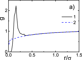
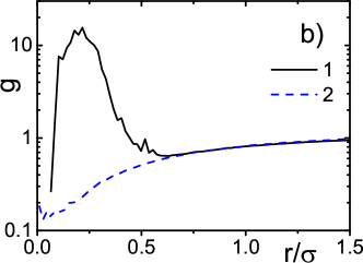
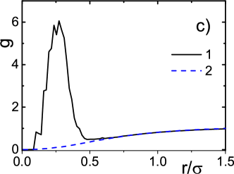
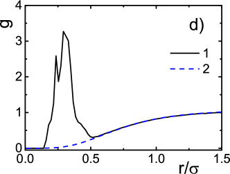
Figure 4: (Color online) The RDFs $g(r/\sigma)$ at $n=0.2$—a); $n=0.6$—b); $n=1.0$—c); $n=1.4$—d). Lines: 1—RDF for the same spin projections; 2—RDF for the opposite spin projections. Small oscillations of the RDFs indicate the Monte-Carlo statistical error.

IV.3 Exchange–correlation bound states

Let us note that the peak on the RDFs for fermions with the same spin projection points out to the increase in the probability to find a fermion between the two ones with the same spin projection at a distance a bit more than the peak position. This third fermion can be considered as located in the well corresponding to the potential of mean force. So these three fermions with the same spin projection can form a three–fermion cluster (TFC) or a triplet. The semiclassical approach is used below to consider the possibility of bound states formation in such a TFC. Analogous exchange–correlation clusters of electrons have been discussed in Weisskopf (1939); Himpsel (2017); Filinov et al. (2021) for a plasma medium and have been identified with three–particle exchange–correlation excitons (see also the collection of theory projects addressing long-standing questions in physics by Prof. Emeritus Franz J. Himpsel Uns ).

The semiclassical approach, which is known to be very effective for many problems of quantum mechanics and mathematical physics, is used below to analyze the possibility of arising bound states in a TFC. For this purpose let us use the Bohr–Sommerfeld condition Nikiforov et al. (2005) for a particle in a spherically symmetric field $w^{(2)}$. According to the definition the PMF is determined up to an arbitrary constant, so to agree with the virial expansion at low density we have to assume here that $w^{(2)}(r)=0$ in the limit $r\rightarrow\infty$. So the Schrödinger equation for the radial part $R(r)$ of the wave function in atomic units looks like:

$$-\frac{1}{2}R^{\prime\prime}+\frac{L(L+1)}{2r^{2}}R-\left(\frac{k_{B}T}{{\rm Ha}}\right)\frac{m_{a}}{m_{e}}\ln(g(r))R\\ {}=\left(\frac{E_{L}}{{\rm Ha}}\right)\frac{m_{a}}{m_{e}}R,$$ (15)

where $E_{L}$ is the energy level, $L=0,1,2,\dots$ is the orbital quantum number Nikiforov et al. (2005), ${\rm Ha}\,m_{e}/(m_{a}k_{B})\approx 57.44\,{\rm K}$. In the semiclassical approximation for a particle in the PMF field $w^{(2)}$, the Bohr–Sommerfeld condition takes the form:

$$\int\limits_{r_{1}(E)}^{r_{2}(E)}p(r){\rm d}r=\pi\left(n_{r}+\frac{1}{2}\right),$$ (16)

where

$$p(r)=\sqrt{2\left[\tilde{E}+\left(\frac{k_{B}T}{{\rm Ha}}\right)\frac{m_{a}}{m_{e}}\ln(g(r))\right]-\frac{(L+\frac{1}{2})^{2}}{r^{2}}},$$ (17)

where $\tilde{E}=\big{(}\frac{E}{{\rm Ha}}\big{)}\frac{m_{a}}{m_{e}}$, $n_{r}$ is the number of zeros of $R(r)$ Nikiforov et al. (2005) and for any energy $E\geq w^{(2)}_{min}$ there are only two turning points $r_{1}$ and $r_{2}$.

Let us consider the results of simulations. Lines 1 and 2 in panels a), b) and c) of Fig. 5 show the PMF $w^{(2)}(r)$ and the sum of $w^{(2)}(r)$ and $\frac{L(L+1/2)}{2r^{2}}$ for $L=1$ . Line 3 in Fig. 5 presents the pseudopotential well created by two neighboring fermions in free space. Differences between $w^{(2)}(r)$ (line 1) and the pseudopotential (line 3) show the influence of the medium on the pseudopotential well.

Let us use the Bohr–Sommerfeld condition Nikiforov et al. (2005) to determine possible bound states in the spherically symmetric field $w^{(2)}$. Our calculations according to (16) show the bound states for $n_{r}=0$ marked by line 4 ($L=0$) in panels a), b), c) and 5 ($L=1$) in panel a) of Fig. 5 for hardnesses $n=0.6,1.0,1.4$ respectively. At $n\mathrel{\hbox to0.0pt{ \lower 4.0pt\hbox{\hskip-3.0pt$\sim$}\hss}\raise 1.0pt\hbox{$<$}}0.6$ and $n\mathrel{\hbox to0.0pt{ \lower 4.0pt\hbox{\hskip-3.0pt$\sim$}\hss}\raise 1.0pt\hbox{$>$}}1.4$ the triplet bound states disappeared.

The momenta corresponding to these bound states can be taken as the average values of $<p(r)>$ in (16) (see lines 1 and 2 in panel d) of Fig. 5). The corresponding bound state momenta are also presented by circles 4 ($L=0$) and 5 ($L=1$) in Fig. 2. Let us stress that the positions of the peaks of the WPIMC MDF agree well enough with the positions of the circles corresponding to the Bohr–Sommerfeld condition, supporting the correctness of our estimations.

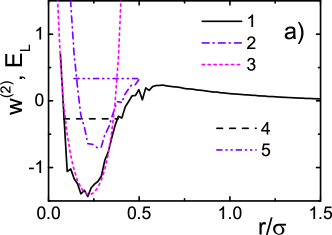
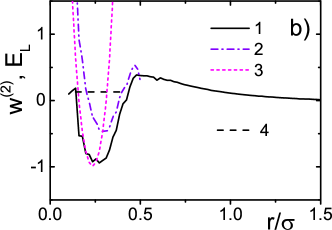
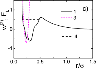
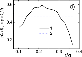
Figure 5: (Color online) PMFs $w^{(2)}(r/\sigma)$ for the same spin projections of fermions. Panels: a)—$n=0.6$; b)—$n=1.0$; c)—$n=1.4$;). Lines: 1—$L=0$; 2—$L=1$; 3—pseudopotential well created by two neighboring fermions in the free space, 4—energy level $E_{L}$ for $n_{r}=0$ and $L=0$; 5—$E_{L}$ for $n_{r}=0$ and $L=1$. Panel d). Typical fermion momenta in the Bohr–Sommerfeld condition. Lines: 1—$p(r)$ in (16); 2—$\langle p(r)\rangle$, average momentum for a bound state corresponding to $n=0.6$, $n_{r}=0$ and $L=0$.

V Discussion

Thermodynamic properties and RDFs of the classical soft–sphere system have been studied many times in the literature for the hardness of the potential larger than three (particularly, for $n=12$, see the review Pieprzyk et al. (2014); Brańka and Heyes (2011)). Here we present the MDFs and RDFs obtained by WPIMC for the hardness of the soft–sphere quantum pseudopotential smaller or of the order of unity ($n=0.2$, 0.6, 1.0, 1.4).

The obtained MDFs demonstrate narrow sharp separated peaks disturbing the Maxwellian distribution. The physical reason for this behavior is the following. The MDFs are averaged over all fermions. The MDF of free fermions is Maxwellian with the average momentum $p\lambda/\hbar\sim 2$ (see Fig. 2). As it follows from the Bohr–Sommerfeld condition the typical momentum of the bound state of a TFC is $p\lambda/\hbar\sim 0.5$. So the peaks on an MDF corresponding to the TFC bound states averaged over all particles with the Maxwellian distribution will be smoothed by the thermal motion. On the contrary, the momentum of slow free fermions with $p\lambda/\hbar\sim 1$ is modified by the momentum of the TFC bound states (of the order of $p\lambda/\hbar\sim 0.5$) so sharp peaks appear in the Maxwellian distribution as it is demonstrated in Figure 2.

To summarize, let us note that the PIMC simulations in the Wigner approach to quantum mechanics used in this paper allow us to calculate the MDFs and the spin–resolved RDFs of a strongly correlated system of soft–sphere fermions for different hardness of the interparticle pseudopotential. The obtained spin–resolved RDFs demonstrate the appearance of three–fermion clusters (triplets) caused by the interference of the exchange and interparticle interactions. The semiclassical analysis in the framework of the Bohr–Sommerfeld quantization condition applied to the PMF corresponding to the same–spin RDF allows to detect the triplet exchange–correlation bound states and to estimate the corresponding averaged energy levels.

References

- Luyten (1971) W. Luyten, Journal of the Royal Astronomical Society of Canada 65, 304 (1971).
- Potekhin (2010) A. Y. Potekhin, Physics-Uspekhi 53, 1235 (2010).
- Boronat et al. (2000) J. Boronat, J. Casulleras, and S. Giorgini, Physica B: Condensed Matter 284, 1 (2000).
- Mazzanti et al. (2003) F. Mazzanti, A. Polls, and A. Fabrocini, Physical Review A 67, 063615 (2003).
- Sesé (2020) L. M. Sesé, Entropy 22, 1338 (2020).
- Nozieres and Pines (2018) P. Nozieres and D. Pines, The Theory of Quantum Liquids: Superfluid Bose Liquids (CRC Press, 2018).
- Feynman and Hibbs (1965) R. P. Feynman and A. R. Hibbs, Quantum Mechanics and Path Integrals (McGraw-Hill, New York, 1965).
- Zamalin et al. (1977) V. Zamalin, G. Norman, and V. Filinov, The monte carlo method in statistical thermodynamics (1977).
- Ebeling et al. (2017) W. Ebeling, V. Fortov, and V. Filinov, Quantum Statistics of Dense Gases and Nonideal Plasmas (Springer, Berlin, 2017).
- Fortov et al. (2020) V. Fortov, V. Filinov, A. Larkin, and W. Ebeling, Statistical physics of Dense Gases and Nonideal Plasmas (PhysMatLit, Moscow, 2020).
- Dornheim et al. (2018) T. Dornheim, S. Groth, and M. Bonitz, Physics Reports 744, 1 (2018).
- Ceperley (1995) D. M. Ceperley, Reviews of Modern Physics 67, 279 (1995).
- Pollock and Ceperley (1984) E. L. Pollock and D. M. Ceperley, Physical Review B 30, 2555 (1984).
- Singer and Smith (1988) K. Singer and W. Smith, Molecular Physics 64, 1215 (1988).
- Filinov et al. (2022a) V. Filinov, R. Syrovatka, and P. Levashov, Molecular Physics p. e2102549 (2022a).
- Ceperley (1991) D. M. Ceperley, Journal of statistical physics 63, 1237 (1991).
- Ceperley (1992) D. M. Ceperley, Physical review letters 69, 331 (1992).
- Wigner (1934) E. Wigner, Physical Review 46, 1002 (1934).
- Tatarskii (1983) V. I. Tatarskii, Soviet Physics Uspekhi 26, 311 (1983).
- Larkin et al. (2017a) A. Larkin, V. Filinov, and V. Fortov, Contributions to Plasma Physics 57, 506 (2017a).
- Larkin et al. (2017b) A. Larkin, V. Filinov, and V. Fortov, Journal of Physics A: Mathematical and Theoretical 51, 035002 (2017b).
- Filinov et al. (2021) V. Filinov, P. Levashov, and A. Larkin, Journal of Physics A: Mathematical and Theoretical 55, 035001 (2021).
- Filinov et al. (2015) V. Filinov, V. Fortov, M. Bonitz, and Z. Moldabekov, Physical Review E 91, 033108 (2015).
- Filinov et al. (2020) V. Filinov, A. Larkin, and P. Levashov, Physical Review E 102, 033203 (2020).
- Filinov et al. (2022b) V. Filinov, A. Larkin, and P. Levashov, Universe 8, 79 (2022b).
- Zamalin and Norman (1973) V. Zamalin and G. Norman, USSR Computational Mathematics and Mathematical Physics 13, 169 (1973).
- Larkin and Filinov (2017) A. Larkin and V. Filinov, Journal of Applied Mathematics and Physics 5, 392 (2017).
- Larkin et al. (2016) A. Larkin, V. Filinov, and V. Fortov, Contributions to Plasma Physics 56, 187 (2016).
- Wiener (1923) N. Wiener, Journal of Mathematics and Physics 2, 131 (1923).
- Demyanov and Levashov (2022) G. Demyanov and P. Levashov, arXiv preprint arXiv:2205.09885 (2022).
- Kelbg (1963) G. Kelbg, Ann. Physik 457, 354 (1963).
- Hansen (1973) J. P. Hansen, Physical Review A 8, 3096 (1973).
- Ebeling et al. (1967) W. Ebeling, H. Hoffmann, and G. Kelbg, Beiträge aus der Plasmaphysik 7, 233 (1967).
- Filinov et al. (2004) A. Filinov, V. Golubnychiy, M. Bonitz, W. Ebeling, and J. Dufty, Phys. Rev. E 70, 04641 (2004).
- Ebeling et al. (2006) W. Ebeling, A. Filinov, M. Bonitz, V. Filinov, and T. Pohl, Journal of Physics A: Mathematical and General 39, 4309 (2006).
- Klakow et al. (1994) D. Klakow, C. Toepffer, and P.-G. Reinhard, The Journal of chemical physics 101, 10766 (1994).
- Kirkwood (1935) J. G. Kirkwood, The Journal of chemical physics 3, 300 (1935).
- Fisher (1964) I. Z. Fisher, Statistical theory of liquids (University of Chicago Press, 1964).
- Zelener et al. (1981) B. Zelener, G. Norman, and V. Filinov, Perturbation theory and pseudopotential in statistical thermodynamics (1981).
- Barker and Henderson (1972) J. Barker and D. Henderson, Annual review of physical chemistry 23, 439 (1972).
- Kirkwood et al. (1950) J. G. Kirkwood, E. K. Maun, and B. J. Alder, The Journal of Chemical Physics 18, 1040 (1950).
- Weisskopf (1939) V. F. Weisskopf, Physical Review 56, 72 (1939).
- Himpsel (2017) F. Himpsel, arXiv preprint arXiv:1701.08080 (2017).
- (44) Unsolved problems in physics, https://uw.physics.wisc.edu/~himpsel/TheoryProjects.html.
- Nikiforov et al. (2005) A. F. Nikiforov, V. G. Novikov, and V. B. Uvarov, Quantum-Statistical Models of Hot Dense Matter: Methods for Computation Opacity and Equation of State, vol. 37 (Springer Science & Business Media, 2005).
- Pieprzyk et al. (2014) S. Pieprzyk, D. Heyes, and A. Brańka, Physical Review E 90, 012106 (2014).
- Brańka and Heyes (2011) A. Brańka and D. Heyes, The Journal of chemical physics 134, 064115 (2011).