ADDP: Learning General Representations for Image Recognition and Generation with Alternating Denoising Diffusion Process

Abstract

Image recognition and generation have long been developed independently of each other. With the recent trend towards general-purpose representation learning, the development of general representations for both recognition and generation tasks is also promoted. However, preliminary attempts mainly focus on generation performance, but are still inferior on recognition tasks. These methods are modeled in the vector-quantized (VQ) space, whereas leading recognition methods use pixels as inputs. Our key insights are twofold: (1) pixels as inputs are crucial for recognition tasks; (2) VQ tokens as reconstruction targets are beneficial for generation tasks. These observations motivate us to propose an Alternating Denoising Diffusion Process (ADDP) that integrates these two spaces within a single representation learning framework. In each denoising step, our method first decodes pixels from previous VQ tokens, then generates new VQ tokens from the decoded pixels. The diffusion process gradually masks out a portion of VQ tokens to construct the training samples. The learned representations can be used to generate diverse high-fidelity images and also demonstrate excellent transfer performance on recognition tasks. Extensive experiments show that our method achieves competitive performance on unconditional generation, ImageNet classification, COCO detection, and ADE20k segmentation. Importantly, our method represents the first successful development of general representations applicable to both generation and dense recognition tasks. Code shall be released.

1 Introduction

Image recognition and image generation are both fundamental tasks in the field of computer vision [2, 26, 59, 41, 17, 31, 56, 18]. Recognition tasks aim to perceive and understand the visual world, while generation tasks aim to create new visual data for various applications. Modern recognition algorithms have already surpassed human performance on many benchmarks [41, 28], and current generative models can synthesize diverse high-fidelity images [49, 22]. However, these two fields have long been developed independently of each other. Recent years have witnessed a significant trend towards general-purpose representation learning. For recognition tasks, researchers have extensively studied general representations that can be adapted to various downstream tasks [44, 20, 26, 10, 53]. Given this unifying trend, it is natural to expect that representations applicable to both recognition and generation tasks could be developed.

Figure 1: Inference pipelines of unified methods that learn general representations for both generation and recognition. Previous methods are modelled either entirely in raw-pixel space or entirely in VQ-token space. In contrast, our method exploits both spaces, yielding competitive performances on both recognition and generation tasks.

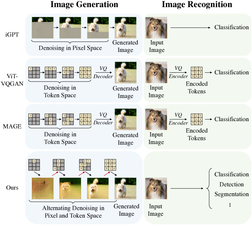
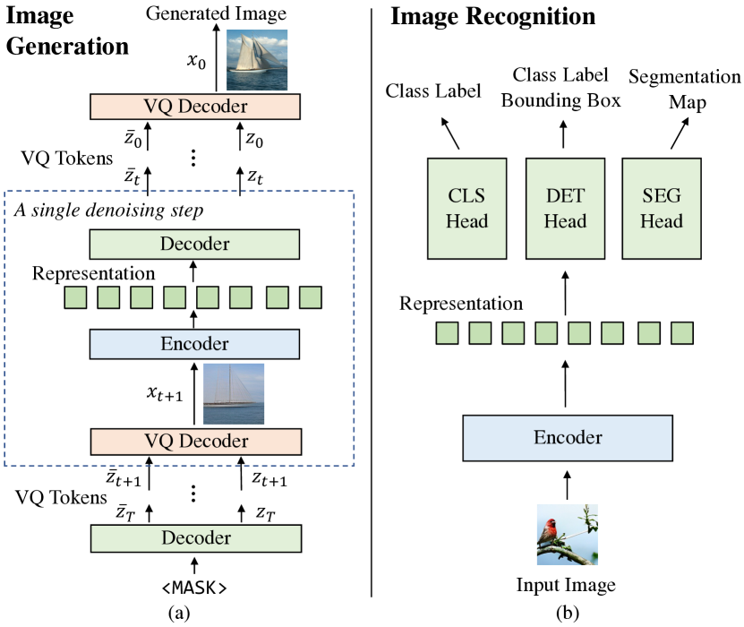
Inspired by this, recent works [38, 60, 8] attempt to learn general representations for both recognition and generation through a specific generative modeling paradigm, i.e., Masked Image Modeling (MIM) [2]. As shown in Fig. 1, during the generation process, they iteratively recover the image content for a portion of masked regions. Such generation process has been leveraged for high-fidelity image synthesis [7]. Meanwhile, each recovery step can be regarded as a special case of MIM using different mask ratios, which has also been proven to learn expressive representations for image recognition [26]. Specifically, ViT-VQGAN [60] and MAGE [38] achieve good generation performance but are still inferior in recognition performance.

We notice that ViT-VQGAN [60] and MAGE [38], like many image generation methods, are modeled in the vector-quantized (VQ) space [57]. While current SOTA representation learning methods for recognition, such as MAE [26] and BEiT [2], all take raw image pixels as inputs. Such observation motivates us to propose the following arguments: (1) Raw pixels as inputs are crucial for recognition tasks. As shown in Tab. 1, taking pixels as inputs outperforms the VQ tokens counterpart in typical recognition tasks. We speculate that this is because VQ tokens lack some image details as well as the spatial sensitivity, which are essential for recognition tasks. (2) VQ tokens as reconstruction targets are beneficial for generation tasks. Previous works such as  [57, 49] show that compared to generating raw pixels, predicting VQ tokens can help the model eliminate imperceptible image details, mitigating the optimization difficulty and resulting in better image generation quality.

Based on these observations, a natural question arises: Is it possible to associate the two spaces within a single representation learning framework, allowing the model to perceive in raw pixels and generate in latent visual tokens?

To this end, we propose a general representation learning framework that bridges pixel and token spaces via an Alternating Denoising Diffusion Process (ADDP). Specifically, at each step in the alternating denoising process, we first decode pixels from previous VQ tokens, and then generate new VQ tokens from these decoded pixels. For the corresponding diffusion process, we first map the original images into VQ-token space with a pre-trained VQ encoder [7], then gradually mask out some VQ tokens. An off-the-shelf VQ decoder is employed for the token-to-pixel decoding, while a learnable encoder-decoder network is introduced for the pixel-to-token generation. The training objective is given by the evidence lower bound (ELBO) of the alternating denoising diffusion process. When applied to image generation, we follow the proposed alternating denoising process to generate images. When applied to image recognition, the learned encoder, which takes raw pixels as inputs, would be fine-tuned on corresponding datasets.

Input	#Params	IN-1k Cls	COCO Det	COCO Det	ADE20k Seg
		$256\times 256$	$256\times 256$	$1024\times 1024$	$256\times 256$
pixel	86M	82.6	29.4	47.5	43.7
token	24M+86M	81.6	12.3	31.0	31.1

Table 1: Performance of taking pixels or tokens as inputs on canonical recognition tasks. We adopt a pre-trained VQ tokenizer [22] to generate the tokens. Under the same training schedule (see Appendix), using VQ-tokens as inputs is inferior to its pixel counterpart on all these tasks.

We demonstrate the superior performance of our method on image generation and recognition tasks, including unconditional generation on ImageNet $256\times 256$ [14], ImageNet-1k classification, COCO [39] detection and ADE20k [63] segmentation. For unconditional generation, our model is able to generate high-fidelity images, achieving better performance than previous state-of-the-art method [38]. For recognition tasks, our model is competitive with current leading methods specifically designed for recognition tasks [26, 2]. It is noteworthy that ADDP is the first approach to develop general representations that are applicable to both generation and dense recognition tasks.

2 Related Work

Deep generative models are initially developed for image generation tasks. But recent research has found that models trained for some specific generative tasks, such as Masked Image Modeling (MIM) [26, 2], have learned expressive representations that can be transferred to various downstream recognition tasks. This discovery has inspired a series of works that attempt to unify image generation and representation learning.

Deep Generative Models for Image Generation.  Early attempts (e.g., GANs [24, 43, 15, 45, 11, 1, 65, 33, 61, 3], VAEs [36, 30, 54], and autoregressive models [55, 56, 52]) directly decode raw pixels from random distributions. However, VQ-VAE [57] points out that directly generating raw pixels is challenging and resource-wasteful due to the redundant low-level information in images. In contrast, VQ-VAE proposes a two-stage paradigm: the first stage encodes images into latent representations (i.e., discrete visual tokens), and the second stage learns to generate visual tokens with powerful autoregressive models. These generated visual tokens are then decoded into raw pixels by the decoder learned in the first stage. Such a two-stage latent space paradigm shows superior training efficiency and performance compared to raw-pixel-wise methods and is thus adopted by most state-of-the-art generative models [48, 60, 22, 25, 7, 47].

On the other hand, diffusion models [31, 17, 25, 47, 7, 50, 6] have also achieved impressive results in image generation, which can produce high-fidelity images by iteratively refining the generated results. For example, Guided Diffusion [17] directly decodes raw pixels with diffusion models, and for the first time achieves better results than GAN- and VAE-based generative models. Recent works (e.g., Stable Diffusion (LDMs) [49], VQ-Diffusion [25] and MaskGIT [7]) further combine diffusion models with the two-stage latent space paradigm, achieving superior image quality. Meanwhile, the success of diffusion models has also been extended to text-to-image generation [25, 47, 50, 6], image editing [62, 35], image denoising [37, 34], etc.

Following state-of-the-art practice, our method also performs diffusion with a latent space to generate images. The difference is that our method alternately refines raw pixels and latent representations, which learns unified representations that can be utilized for both recognition and generation tasks with competitive performance.

Generative Pre-training for Image Representation Learning.  Recent research [2, 44, 20, 26, 10, 40, 59, 23] suggest that some specific generative modeling tasks (e.g., Masked Image Modeling (MIM)) can learn more expressive and effective representations than previous representation learning methods (e.g., supervised methods [21, 41] and self-supervised discriminative methods [27, 12, 9]). These generative pre-training methods have shown superior performance when transferred to various downstream recognition tasks, such as image classification, object detection, and semantic segmentation. MIM methods learn representations by reconstructing image content from masked images. For example, BEiTs [2, 44, 20] reconstruct the discrete visual tokens corresponding to masked parts. MAEs [26, 10] directly reconstruct the masked pixels. Some works [40, 59] also attempt to reconstruct the momentum features of the original images. Apart from these MIM methods, Corrupted Image Modeling (CIM) [23] learns representations by reconstructing from corrupted images, which eliminates the use of artificial mask tokens that never appear in the downstream fine-tuning stage.

These generative pre-training methods only focus on the representational expressiveness for image recognition. They do not care about the quality of reconstructed images and cannot be directly used for image generation tasks. In contrast, our method learns general representations that perform well for both image recognition and generation tasks.

Generative Modeling for Unifying Representation Learning and Image Generation.  Early attempts [18, 19] consider representation learning and image generation as dual problems, thus learning two independent networks (i.e., an image encoder and an image generator) to solve both tasks at the same time in a dual-learning paradigm. Inspired by generative representation learning for natural language [16, 46, 32], iGPT [8] for the first time unifies these two tasks into a single network by learning from autoregressive image generation, providing good performance for both image recognition and image generation tasks. To further improve performance, ViT-VQGAN [60] replaces the raw-pixel inputs and outputs with discrete visual tokens. Recently, MAGE [38] proposes to replace the autoregressive decoding process with a diffusion method (i.e., MaskGIT [7]), following state-of-the-art practices for image generation.

Despite these attempts at unifying representation learning and image generation, their recognition performance is still inferior to state-of-the-art representation learning methods. They perform representation learning either entirely in raw-pixel space or entirely in latent space. In contrast, our method exploits both raw-pixel and latent space, learning general representations that yield competitive performance on both image recognition and image generation tasks.

3 Method

Figure 2: Alternating denoising process. Our method first predicts $p_{\theta}(z_{T},\bar{z}_{T}|\varnothing)$ by directly feeding all <MASK> tokens into our decoder $D_{\theta}$ in Eq. (2). At each step $t$, the noisy image $x_{t}$ is decoded according to Eq. (1), then used to generate new reliable tokens $z_{t-1}$ and unreliable tokens $\bar{z}_{t-1}$ according to Eq. (2). $x_{0}$ is the final synthesized noisy-free image.

3.1 Alternating Denoising of Pixels and VQ tokens

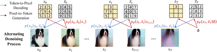
As stated before, raw pixels are crucial for recognition tasks, while VQ tokens are beneficial for generation tasks. Therefore, instead of performing the denoising process entirely in raw-pixel space or VQ-token space as previous works [60, 38, 17], we propose to denoise pixels and VQ tokens alternately. As shown in Fig. 2, in each step, we first decode pixels from previously generated VQ tokens, then generate new VQ tokens conditioned on decoded pixels. Denoising from pixels facilitates representation learning for recognition tasks. In addition, the reconstruction in VQ space helps generate diverse high-fidelity images.

Similar to previous diffusion methods for image generation [25, 38], the VQ token denoising process starts with an empty sequence and gradually adds new reliable VQ tokens step-by-step. Suppose $z_{t}$ is the reliable VQ sequence at step $t$, then $z_{t-1}$ would add new reliable VQ tokens to $z_{t}$. On the other hand, the raw pixels denoising process starts with a full image $x_{T}$ that is entirely noisy, then gradually refines the noisy image to a noise-free high-fidelity image $x_{0}$. To enable the alternating denoising process and associate the two spaces, token-to-pixel decoding and pixel-to-token generation are introduced as follows.

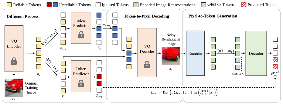
Token-to-Pixel Decoding is widely used in image generation to restore the generated VQ tokens to visual image pixels [57, 22, 7]. The VQ decoder subnetworks in off-the-shelf pre-trained VQ tokenizers (e.g., VQGAN [22]) could be directly used to perform such decoding. However, the existing VQ decoders only support decoding images from the complete VQ sequences and cannot accept partial VQ tokens as inputs. In contrast, the denoising process can only generate a portion of reliable VQ tokens at each step. To resolve this inconsistency and facilitate the use of off-the-shelf VQ decoders, we propose to pair the reliably generated VQ tokens $z_{t}$ at step $t$ with unreliable VQ tokens $\bar{z}_{t}$. Then, the conditional probability of decoded image $x_{t}$ given the reliable tokens $z_{t}$ and unreliable token $\bar{z}_{t}$ is defined as

$$\begin{split}p(x_{t}|z_{t},\bar{z}_{t})=&\\ \delta\Big{[}x_{t}=\mathrm{VQ}&\text{-}\mathrm{Decoder}\big{(}z_{t}\odot(1-m_{t})+\bar{z}_{t}\odot m_{t}\big{)}\Big{]},\end{split}$$ (1)

where $\odot$ is the element-wise product. $m_{t}$ is a binary mask indicating the unreliable regions derived from $z_{t}$. $m_{t}$ shares the same spatial size with $z_{t}$ and $\bar{z}_{t}$, where the regions with binary values of 1 are unreliable. Both the reliable VQ tokens $z_{t}$ and unreliable VQ tokens $\bar{z}_{t}$ would be predicted by our models, which will be discussed in Sec. 3.3.

Pixel-to-Token Generation has been shown to be effective for recognition tasks in recent representation learning works [2, 44, 20]. Our method introduces a learnable encoder-decoder network to recover unreliable VQ tokens from noisy images to enable representation learning from pixels. As shown in Fig. 4, the previously decoded noisy full images $x_{t}$ at step $t$ are used as network inputs. The encoder subnetwork extracts representation $e_{t}$ from $x_{t}$. Before feeding into the decoder, following previous MIM methods, the unreliable regions (i.e., $m_{t}=1$) of the extracted representation $e_{t}$ would be replaced with learnable <MASK> token embedding. The decoder will predict $z_{t-1}$ and $\bar{z}_{t-1}$ of the next step based on these inputs. Then, given the noisy image $x_{t}$, the conditional probability of generated reliable VQ tokens $z_{t-1}$ and unreliable VQ tokens $\bar{z}_{t-1}$ at the next step $t-1$ are given as

$$\begin{split}p_{\theta}(z_{t-1},\bar{z}_{t-1}|x_{t})=&\\ D_{\theta}\Big{(}E_{\theta}(x_{t})&\odot(1-m_{t})+e_{\mathrm{mask}}\odot m_{t}\Big{)},\end{split}$$ (2)

where $m_{t}$ is the same binary mask as in Eq. (1), indicating the unreliable regions at step $t$. $E_{\theta}$ and $D_{\theta}$ are learnable encoder and decoder subnetworks with parameters $\theta$, respectively. $e_{\mathrm{mask}}$ is a learnable <MASK> token embedding. Since full images are fed into the encoder as inputs, our method can employ various image encoding networks (e.g., CNNs [28] and ViTs [21]). Experiments in Sec. 4.2 show that the learned representations extracted from the encoder perform well for both recognition and generation tasks.

Alternating Denoising Process is shown in Fig. 2. Starting from the empty sequence with the unreliable mask $m_{T+1}$ of all $1$s, $p_{\theta}(z_{T},\bar{z}_{T}|\varnothing)$ is predicted by feeding all <MASK> tokens into our decoder $D_{\theta}$ in Eq. (2). Then, at each step $t$, the noisy images $x_{t}$ are decoded according to Eq. (1) and then used to generate new reliable tokens $z_{t-1}$ and unreliable tokens $\bar{z}_{t-1}$ according to Eq. (2). Finally, the synthesized noisy-free images are the refined images $x_{0}$ at step $0$. The joint distribution of all variables in the alternating denoising process can be described as

$$\begin{split}p_{\theta}(z_{0:T},&\bar{z}_{0:T},x_{0:T})=\color[rgb]{0,0,1}\definecolor[named]{pgfstrokecolor}{rgb}{0,0,1}\underbrace{\color[rgb]{0,0,0}\definecolor[named]{pgfstrokecolor}{rgb}{0,0,0}\pgfsys@color@gray@stroke{0}\pgfsys@color@gray@fill{0}p_{\theta}(z_{T},\bar{z}_{T}|\varnothing)}_{\text{our model}}~{}\color[rgb]{0,0,1}\definecolor[named]{pgfstrokecolor}{rgb}{0,0,1}\underbrace{\color[rgb]{0,0,0}\definecolor[named]{pgfstrokecolor}{rgb}{0,0,0}\pgfsys@color@gray@stroke{0}\pgfsys@color@gray@fill{0}p(x_{0}|z_{0})}_{\text{VQ-Decoder}}\\ &\cdot\prod_{t=0}^{T-1}\color[rgb]{0,0,1}\definecolor[named]{pgfstrokecolor}{rgb}{0,0,1}\underbrace{\color[rgb]{0,0,0}\definecolor[named]{pgfstrokecolor}{rgb}{0,0,0}\pgfsys@color@gray@stroke{0}\pgfsys@color@gray@fill{0}p(x_{t+1}|z_{t+1},\bar{z}_{t+1})}_{\text{VQ-Decoder}}~{}\color[rgb]{0,0,1}\definecolor[named]{pgfstrokecolor}{rgb}{0,0,1}\underbrace{\color[rgb]{0,0,0}\definecolor[named]{pgfstrokecolor}{rgb}{0,0,0}\pgfsys@color@gray@stroke{0}\pgfsys@color@gray@fill{0}p_{\theta}(z_{t},\bar{z}_{t}|x_{t+1})}_{\text{our model}}.\end{split}$$ (3)

3.2 Diffusion Process

Figure 3: Diffusion process. First, the original image $x_{0}$ is encoded to VQ tokens $z_{0}$. Then, the diffusion process masks out some VQ tokens based on a Markov chain $q(z_{t+1}|z_{t})$. As mentioned in Sec. 3.1, $z_{t}$ corresponds to the reliable VQ tokens, while $\bar{z}_{t}$ is the unreliable VQ tokens used as inputs for the VQ decoder in Eq. (1), which is sampled from the conditional distribution $q(\bar{z}_{t}|z_{t+1})$.

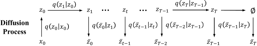
Following the previous denoising diffusion training paradigm [25], a corresponding diffusion process needs to be defined (see Fig. 3). Given a training image $x_{0}$, an off-the-shelf pre-trained VQ encoder is used to map $x_{0}$ to its corresponding VQ tokens $z_{0}=\mathrm{VQ\text{-}Encoder}(x_{0})$. Then, the diffusion process gradually masks out some regions of the VQ tokens with a Markov chain $q(z_{t+1}|z_{t})$. As mentioned in Sec. 3.1, $z_{t}$ corresponds to the reliable VQ tokens at step $t$. $z_{t+1}$ contains only a part of reliable VQ tokens in $z_{t}$. The diffusion process consists of $T+1$ steps, where all tokens would be masked out at step $T+1$.

For the unreliable VQ tokens $\bar{z}_{t}$ used as inputs for the VQ decoder in Eq. (1), the conditional distribution during diffusion is defined as $q(\bar{z}_{t}|z_{t+1})$. Note that, instead of $z_{t}$, the reliable tokens $z_{t+1}$ at step $t+1$ are used as the condition. That is because during denoising, $\bar{z}_{t}$ and $z_{t}$ are conditionally independent given $x_{t}$, it is intractable to predict $q(\bar{z}_{t}|z_{t})$ from $x_{t}$. Experiments in Tab. 4 also demonstrate the superiority of using $q(\bar{z}_{t}|z_{t+1})$ over $q(\bar{z}_{t}|z_{t})$ in the diffusion process. The optimal value of $q(\bar{z}_{t}|z_{t+1})$ should be $q(z_{0}|z_{t+1})$, because samples from $q(z_{0}|z_{t+1})$ give the most reliable VQ tokens. However, $q(z_{0}|z_{t+1})$ is generally intractable. To alleviate this issue, the distribution of unreliable tokens $\bar{z}_{t}$ is defined as

$$q(\bar{z}_{t}|z_{t+1})=\hat{p}_{z_{0}|z_{t+1}}(\bar{z}_{t}),$$ (4)

where $\hat{p}_{z_{0}|z_{t+1}}(\cdot)$ is an off-the-shelf token predictor pre-trained to predict $q(z_{0}|z_{t+1})$. Note that the token predictor is only adopted during training and abandoned in inference. Then, the whole diffusion process is described as

$$\begin{split}q(z_{0:T},\bar{z}_{0:T}|x_{0})=&\color[rgb]{0,0,1}\definecolor[named]{pgfstrokecolor}{rgb}{0,0,1}\underbrace{\color[rgb]{0,0,0}\definecolor[named]{pgfstrokecolor}{rgb}{0,0,0}\pgfsys@color@gray@stroke{0}\pgfsys@color@gray@fill{0}q(z_{0}|x_{0})}_{\text{VQ-Encoder}}\color[rgb]{0,0,1}\definecolor[named]{pgfstrokecolor}{rgb}{0,0,1}\underbrace{\color[rgb]{0,0,0}\definecolor[named]{pgfstrokecolor}{rgb}{0,0,0}\pgfsys@color@gray@stroke{0}\pgfsys@color@gray@fill{0}q(\bar{z}_{T}|\varnothing)}_{\text{token predictor}}\\ &\cdot\prod_{t=0}^{T-1}\color[rgb]{0,0,1}\definecolor[named]{pgfstrokecolor}{rgb}{0,0,1}\underbrace{\color[rgb]{0,0,0}\definecolor[named]{pgfstrokecolor}{rgb}{0,0,0}\pgfsys@color@gray@stroke{0}\pgfsys@color@gray@fill{0}q(z_{t+1}|z_{t})}_{\text{add mask}}\color[rgb]{0,0,1}\definecolor[named]{pgfstrokecolor}{rgb}{0,0,1}\underbrace{\color[rgb]{0,0,0}\definecolor[named]{pgfstrokecolor}{rgb}{0,0,0}\pgfsys@color@gray@stroke{0}\pgfsys@color@gray@fill{0}q(\bar{z}_{t}|z_{t+1})}_{\text{token predictor}}.\end{split}$$ (5)

For simplicity, the decoded noisy images $x_{1:T}$ are omitted, since the derivation of the training objective (refer to Appendix) shows that they are unnecessary to be included in the diffusion process.

Figure 4: Training pipeline of our framework. First, the original training image $x_{0}$ is encoded into VQ token $z_{0}$. Then, a certain timestep $t$ is sampled. The reliable and unreliable tokens $z_{t}$ and $\bar{z}_{t}$ are generated according to the diffusion process in Sec. 3.2. After that, $x_{t}$ is decoded by token-to-pixel decoding in Sec. 3.1. Our pixel-to-token generation network takes $x_{t}$ as input and generate the prediction of $\bar{z}_{t-1}$. $q(\bar{z}_{t-1}|z_{t})$ is used as the training target as mentioned in Sec. 3.3.

Figure 5: Inference pipeline of our model for image generation and recognition. For generation, our model predicts $z_{t}$ and $\bar{z}_{t}$ at each denoising step given the noisy image $x_{t+1}$. For recognition, the encoder of our model can be directly transferred to various downstram tasks, including classification, detection and segmentation.

3.3 Learning the Denoising Process

Given the proposed alternating denoising diffusion process, our model can be optimized to minimize the evidence lower bound (ELBO) of $\log p_{\theta}(x_{0})$. Concretely, the training objectives can be divided into the following terms (see Appendix for derivation)

$$L_{\mathrm{ELBO}}=L_{\mathrm{VQ}}+\sum_{t=0}^{T-1}L_{t}+L_{T},$$ (6)

$$L_{\mathrm{VQ}}=\mathbb{E}_{q(z_{0},\bar{z}_{0},x_{0})}\Big{[}-\log\color[rgb]{0,0,1}\definecolor[named]{pgfstrokecolor}{rgb}{0,0,1}\underbrace{\color[rgb]{0,0,0}\definecolor[named]{pgfstrokecolor}{rgb}{0,0,0}\pgfsys@color@gray@stroke{0}\pgfsys@color@gray@fill{0}p(x_{0}|z_{0})}_{\text{VQ-Decoder}}+\log\color[rgb]{0,0,1}\definecolor[named]{pgfstrokecolor}{rgb}{0,0,1}\underbrace{\color[rgb]{0,0,0}\definecolor[named]{pgfstrokecolor}{rgb}{0,0,0}\pgfsys@color@gray@stroke{0}\pgfsys@color@gray@fill{0}q(z_{0}|x_{0})}_{\text{VQ-Encoder}}\Big{]},$$

$$\begin{aligned} L_{t}=&\mathbb{E}_{q(z_{t+1},\bar{z}_{t+1},z_{0})}\Big{[}D_{\mathrm{KL}}\Big{(}q(z_{t}|z_{t+1},z_{0})\color[rgb]{0,0,1}\definecolor[named]{pgfstrokecolor}{rgb}{0,0,1}\underbrace{\color[rgb]{0,0,0}\definecolor[named]{pgfstrokecolor}{rgb}{0,0,0}\pgfsys@color@gray@stroke{0}\pgfsys@color@gray@fill{0}q(\bar{z}_{t}|z_{t+1})}_{\text{token predictor}}~{}||\\ &\qquad\color[rgb]{0,0,1}\definecolor[named]{pgfstrokecolor}{rgb}{0,0,1}\underbrace{\color[rgb]{0,0,0}\definecolor[named]{pgfstrokecolor}{rgb}{0,0,0}\pgfsys@color@gray@stroke{0}\pgfsys@color@gray@fill{0}p_{\theta}(z_{t},\bar{z}_{t}|x_{t+1}=\mathrm{VQ\text{-}Decoder}(z_{t+1},\bar{z}_{t+1}))}_{\text{our model}}\Big{)}\Big{]},\end{aligned}$$

$$L_{T}=\mathbb{E}_{q(z_{0})}\Big{[}D_{\mathrm{KL}}\Big{(}q(z_{T}|z_{0})\color[rgb]{0,0,1}\definecolor[named]{pgfstrokecolor}{rgb}{0,0,1}\underbrace{\color[rgb]{0,0,0}\definecolor[named]{pgfstrokecolor}{rgb}{0,0,0}\pgfsys@color@gray@stroke{0}\pgfsys@color@gray@fill{0}q(\bar{z}_{T}|\varnothing)}_{\text{token predictor}}||\color[rgb]{0,0,1}\definecolor[named]{pgfstrokecolor}{rgb}{0,0,1}\underbrace{\color[rgb]{0,0,0}\definecolor[named]{pgfstrokecolor}{rgb}{0,0,0}\pgfsys@color@gray@stroke{0}\pgfsys@color@gray@fill{0}p_{\theta}(z_{T},\bar{z}_{T}|\varnothing)}_{\text{our model}}\Big{)}\Big{]},$$

where $D_{\mathrm{KL}}$ is KL divergence. $L_{\mathrm{VQ}}$ corresponds to the training of VQ tokenizer, which is omitted in our training because a pre-trained VQ tokenizer is used. $L_{0:T}$ are used to optimize our model parameters $\theta$. $p_{\theta}$ is given by Eq. (2).

Training Target.  Like previous MIM methods [26, 2], we only optimize the loss $L_{t}$ on masked tokens (i.e., unreliable regions with $m_{t+1}=1$). Following the reparameterization trick in VQ-Diffusion [25], $L_{t}$ can be further simplified as (see Appendix for derivation)

$$L_{t}= \mathbb{E}_{q(z_{t+1},\bar{z}_{t+1})}\Big{[}D_{\mathrm{KL}}\Big{(}q(z_{0}|z_{t+1})\color[rgb]{0,0,1}\definecolor[named]{pgfstrokecolor}{rgb}{0,0,1}\underbrace{\color[rgb]{0,0,0}\definecolor[named]{pgfstrokecolor}{rgb}{0,0,0}\pgfsys@color@gray@stroke{0}\pgfsys@color@gray@fill{0}q(\bar{z}_{t}|z_{t+1})}_{\text{token predictor}}~{}||$$ (7)

$$\qquad\color[rgb]{0,0,1}\definecolor[named]{pgfstrokecolor}{rgb}{0,0,1}\underbrace{\color[rgb]{0,0,0}\definecolor[named]{pgfstrokecolor}{rgb}{0,0,0}\pgfsys@color@gray@stroke{0}\pgfsys@color@gray@fill{0}p_{\theta}(z_{0},\bar{z}_{t}|x_{t+1}=\mathrm{VQ\text{-}Decoder}(z_{t+1},\bar{z}_{t+1}))}_{\text{our model}}\Big{)}\Big{]},$$

which implies that $q(z_{0}|z_{t+1})$ and $q(\bar{z}_{t}|z_{t+1})$ are the training targets of our model. However, $q(z_{0}|z_{t+1})$ is generally intractable. We notice that the token predictor $q(\bar{z}_{t}|z_{t+1})$ is actually an estimation of $q(z_{0}|z_{t+1})$ according to Eq. (4). Therefore, it is feasible to predict $q(\bar{z}_{t}|z_{t+1})$ only. We adopt such a design in practice. Fig. 4 shows the training process.

Training Input.  Our model $p_{\theta}$ takes the noisy synthesized image $x_{t}=\mathrm{VQ\text{-}Decoder}(z_{t},\bar{z}_{t})$ as training inputs. Inappropriate values of unreliable $\bar{z}_{t}$ may hurt the quality of synthesized images, degenerating the performance of image generation and image recognition tasks.

To alleviate this issue, instead of directly use $\bar{z}_{t}$ sampled from $\hat{p}_{z_{0}|z_{t+1}}(\bar{z}_{t})$ in Eq. (4), we propose to use $f(\hat{p}_{z_{0}|z_{t+1}})$ for the unreliable parts in Eq. (1) as

$$x_{t}=\mathrm{VQ\text{-}Decoder}\big{(}z_{t}\odot(1-m_{t})+f(\hat{p}_{z_{0}|z_{t+1}})\odot m_{t}\big{)},$$ (8)

where $\hat{p}_{z_{0}|z_{t+1}}\in[0,1]^{C}$ is the complete distribution vector predicted by the token predictor. $C$ is the codebook size of the VQ tokenizer. $f(\cdot)$ is a mapping function designed to mitigate the inaccurate estimation of $\hat{p}_{z_{0}|z_{t+1}}$. Candidates for the mapping function $f(\cdot)$ are designed as $\{\mathrm{Sampling},~{}\mathrm{ArgMax},~{}\mathrm{WeightedSum}\}$. $\mathrm{Sampling}$ is the naïve design that sample tokens according to $\hat{p}_{z_{0}|z_{t+1}}$. $\mathrm{ArgMax}$ is to choose the tokens with the largest probability in $\hat{p}_{z_{0}|z_{t+1}}$. $\mathrm{WeightedSum}$ indicates directly feeding the soft distribution $\hat{p}_{z_{0}|z_{t+1}}$ into VQ decoder. All VQ embeddings within the token codebook would be weighted summed accoding to the soft distribution before fed into the VQ decoder network. Empirically, we find that using $\mathrm{WeightedSum}$ mapping produces high-quality images and helps to improve our model performance (see Sec. 4.3).

In practice, we also find that feeding the reliable tokens $z_{t}$ into our decoder $D_{\theta}$ as the additional information benefits both recognition and generation tasks. We suspect predicting VQ tokens only from images with considerable noise is difficult when the mask ratio is relatively large.

Apply to Image Generation.  For image generation, we follow the denoising process mentioned in Sec. 3.1 and Fig. 5 (a). Starting from an empty sequence, our model predicts $z_{T}$ and $\bar{z}_{T}$ from pure <MASK> token embeddings. At each step, the VQ decoder generate $x_{t+1}$ from tokens of current step $z_{t+1}$ and $\bar{z}_{t+1}$. Then, the pixels $x_{t+1}$ are fed into our encoder-decoder network to predict $z_{t}$ and $\bar{z}_{t}$ of the next step. $x_{0}$ is the final generated noisy-free image.

Apply to Image Recognition.  After pre-training, our model can be applied to various recognition tasks, as shown in Fig. 5 (b). For recognition tasks, the encoder takes raw pixels as input. The encoded representations can be forwarded to different task-specific heads. After fine-tuning on corresponding datasets, our model delivers strong performances on a wide range of tasks (see Sec. 4.2).

4 Experiments

Method	#Params.	Uncond. Gen.		#Params.	ImageNet		COCO		ADE20k
	Gen.	FID$\downarrow$	IS$\uparrow$	Rec.	FT$\uparrow$	Linear$\uparrow$	AP${}^{\text{box}}$$\uparrow$	AP${}^{\text{mask}}$$\uparrow$	mIoU$\uparrow$
Designed for Recognition Only
MoCo v3 [13]	-	-	-	86M	83.0	76.7	47.9	42.7	47.3
DINO [4]	-	-	-	86M	83.3	77.3	46.8	41.5	47.2
BEiT [2]	-	-	-	86M	83.2	37.6	49.8	44.4	47.1
CIM [23]	-	-	-	86M	83.3	-	-	-	43.5
MAE [26]	-	-	-	86M	83.6	68.0	51.6	45.9	48.1
CAE [10]	-	-	-	86M	83.9	70.4	50.0	44.0	50.2
iBOT [64]	-	-	-	86M	84.0	79.5	51.2	44.2	50.0
SiameseIM [53]	-	-	-	86M	84.1	78.0	52.1	46.2	51.1
Designed for Generation Only
BigGAN [19]	$\sim$70M	38.6	24.70	-	-	-	-	-	-
ADM [17]	554M	26.2	39.70	-	-	-	-	-	-
MaskGIT [7]	203M	20.7	42.08	-	-	-	-	-	-
IC-GAN [5]	$\sim$77M	15.6	59.00	-	-	-	-	-	-
Designed for Both Recognition and Generation
iGPT-L [8]	1362M	-	-	1362M	72.6	65.2	-	-	-
ViT-VQGAN [60]	650M	-	-	650M	-	65.1	-	-	-
MAGE [38]	86M+90M	11.0∗	95.42∗	86M+24M	82.5	74.7	-	-	-
Ours	86M+90M	8.9	95.32	86M	83.9	11.5	51.7	45.8	48.1

Table 2: Comparison of ADDP with different kinds of existing methods on both visual recognition and generation tasks. The FID [29], IS [51] of unconditional image generation (denoted by Uncond. Gen.) is evaluated on ImageNet-1k [14] 256$\times$256 validation set; The top-1 accuracy of fine-tuning (FT) and linear probing (Linear) is reported on ImageNet-1k [14]. AP${}^{\text{box}}$ and AP${}^{\text{mask}}$ is reported on COCO [39] test-dev set. mIoU is reported on ADE20k [63] validation set. #Params. Gen. and #Params. Rec. denote the total number of parameters for unconditional generation and recognition backbone, respectively.
* The generation performance of MAGE is re-evaluated using our inference strategy for fair comparasion. The original FID and IS scores of MAGE are 11.1 and 81.17, respectively. The results of our method are marked in gray.

4.1 Implementation Details

Network. We adopt the VQ tokenizer from the off-the-shelf VQGAN [22, 7] model released by MAGE [38]. MAGE Base model is used as the token predictor in Eq. (4). Note that the MAGE model is only used in training, but not in inference. We adopt a ViT-Base [21] model as the encoder, and use 8 Transformer [58] blocks of 768 feature dimension as the decoder. For the decoder inputs, we use three sets of separate learnable positional embeddings for pixels, tokens and <MASK> tokens.

Training. Our models are trained on ImageNet-1k [14] dataset. The total number of denoising steps is set as $T=100$. For masking strategy, we sample step $t$ from the values of 1, 2, $\dots$, $T$, while ensuring the mask ratio distribution close to that of MAGE [38] for a fair comparison. To accommodate our model with different denoising steps in inference, we further sample $\Delta t$ from a uniform discrete distribution over 1 to 5. $z_{t+\Delta t}$ is used to replace $z_{t+1}$. AdamW [42] optimizer with a peak learning rate of $1.5\times 10^{-3}$ is used. The model is trained for 1600 epochs with 40 warmup epochs and batch size of 4096. Please see Appendix for more details.

Image Recognition. The transfer performance of image classification on ImageNet-1k [14], object detection on COCO [39] and semantic segmentation on ADE20k [63] are used for evaluation. We use the pre-trained encoder as backbone and append task-specific heads for different tasks. Please see Appendix for more details.

Image Generation. After training, we use iterative decoding as in MaskGIT [7] to iteratively fill in masked tokens and generate images. By default, we recover one token per step. Please see Appendix for more details and the generated images by our method.

4.2 Main Results

In Tab. 2, our method is compared with previous methods designed for recognition only, generation only, or both recognition and generation.

Unconditional Generation. Our method surpasses the previous best by $\sim 2$ FID. This validates the effectiveness of our proposed alternating denoising process in generating high-quality images. Our method incorporates the raw-pixel space into the denoising process, which was previously considered a challenging task [57, 49]. Please see Appendix for the generated images by our method.

Image Classification. Our model achieves comparable fine-tuning performance with methods specifically designed for recognition. Moreover, compared with the previously best method (i.e., MAGE [38]) designed for both recognition and generation, our model boosts the performance by $1.4$ points. This is consistent with the conclusion drawn from Tab. 1, suggesting pixel inputs are more friendly with recognition tasks. Interestingly, the linear probing accuracy is very low. We suspect this is because our models are learned from noisy synthetic images, which are far from natural images and have not been well explored in previous studies. Please see Appendix for the noisy synthetic images used for training.

Object Detection and Semantic Segmentation. Benefiting from our alternating denoising diffusion process, our model is successfully applied to object detection and semantic segmentation. As far as we know, this is the first work demonstrating that general representations can be learned for both generation and dense prediction tasks. Our method demonstrates competitive performance with previous methods specifically designed for recognition. We note that iBOT [64] and SiameseIM [53] incorporate contrastive learning with MIM to boost the final performance. Our model may also benefit from a similar mechanism.

4.3 Ablation Study

Ablation setting. Our model is trained for 150 epochs in ablation studies. We report the FID [29] and IS [51] scores of unconditional generation with $20$ inference steps as well as the fine-tuning accuracy (FT) on ImageNet-1k [14]. Default settings are marked in gray.

Probability Condition for Unreliable Tokens.  As mentioned in Sec. 3.2, the prediction of $\bar{z}_{t}$ is conditioned on $z_{t+1}$ rather than $z_{t}$. Tab. 3 verifies that using $z_{t}$ as condition leads to poor generation performance.

Mapping Function for Unreliable Tokens.  As noted in Eq. (8), proper mapping function choices can help improve the quality of the learned representation. Different designs are compared in Tab. 4. It is shown that directly $\mathrm{Sampling}$ is inferior in both generation and classification, while $\mathrm{WeightedSum}$ can deliver sound performance.

Token Input.  Directly recovering tokens from pixels with considerable noise may be challenging when the mask ratio is extremely high. Tab. 5 shows the effect of feeding tokens to our model. It demonstrates that feeding tokens can greatly enhance the generation ability. However, if tokens are fed through the encoder, the classification results declines severely. We suspect that the model may focus only on tokens in this setting, because it may be easier to recover tokens in the same space.

Prediction Target. As discussed in Sec. 3.3, there are two possible target for training networks: $q(z_{0}|z_{t+1})$ and $q(\bar{z}_{t}|z_{t+1})$. While $q(z_{0}|z_{t+1})$ can not be computed directly, we try to sample $z_{0}$ as an estimated target. Tab. 6 studies the effect of targets. The results show that predicting $q(\bar{z}_{t}|z_{t+1})$ is better on both generation and classification tasks.

Inference Strategy for Image Generation. Tab. 7 studies the effect of inference strategies. Previous works [7, 38] adopt cosine masking schedule in inference. With this schedule, we find that the generation results quickly get saturated with more inference steps. We also try the linear masking schedule in inference. It is shown to provide consistent gain as $T$ becomes larger.

Conditional	FID $\downarrow$	IS $\uparrow$	FT $\uparrow$
Probability
$q(\bar{z}_{t}|z_{t})$	80.75	13.48	83.7
$q(\bar{z}_{t}|z_{t+1})$	23.63	33.09	83.5

Table 3: Ablation on condition for unreliable tokens.

Mapping Function $f(\cdot)$	FID $\downarrow$	IS $\uparrow$	FT $\uparrow$
$\mathrm{Sampling}$	38.79	23.44	83.2
$\mathrm{ArgMax}$	26.62	30.03	83.5
$\mathrm{WeightedSum}$	23.63	33.09	83.5

Table 4: Ablation on mapping function $f(\cdot)$.

Token Input	FID $\downarrow$	IS $\uparrow$	FT $\uparrow$
encoder & decoder	20.40	37.20	81.5
decoder-only	23.63	33.09	83.5
None	36.24	21.71	83.1

Table 5: Ablation on token input strategy.

Prediction	Masking	FID $\downarrow$	IS $\uparrow$	FT $\uparrow$
Target	Strategy
$q(\bar{z}_{t}|z_{t+1})$	default	23.63	33.09	83.5
$\delta(\hat{z}_{0}=z_{0})$	default	39.41	18.62	83.2
$\delta(\hat{z}_{0}=z_{0})$ & $q(\bar{z}_{t}|z_{t+1})$	default	30.43	23.40	83.5
$\delta(\hat{z}_{0}=z_{0})$	fixed (50%)	166.54	4.73	83.4

Table 6: Ablation on prediction target and masking ratio.

Masking	Inference Steps T	FID $\downarrow$	IS $\uparrow$
Schedule
cosine	20	16.82	49.45
cosine	50	11.35	70.05
cosine	100	10.54	82.90
cosine	200	10.62	94.26
linear	64	11.02	68.06
linear	128	9.15	80.58
linear	256	8.94	95.32

Table 7: Ablation on masking schedule and inference steps $T$ during generation inference.

5 Conclusions

In this paper, we introduce ADDP, a general representation learning framework that is applicable to both image generation and recognition tasks. Our key insights are twofold: (1) pixels as inputs are crucial for recognition tasks; (2) VQ tokens as reconstruction targets are beneficial for generation tasks. To meet the demands of both fields, we propose an Alternating Diffusion Denoising Process (ADDP) to bridge pixel and token spaces. Our network is trained to optimize the evidence lower bound (ELBO). Extensive experiments demonstrate its superiority in image generation and recognition tasks. ADDP demonstrates that, for the first time, a general representation can be learned for both generation and dense recognition tasks.

Acknowledgements.  The work is partially supported by the National Key R&D Program of China under Grants 2022ZD0114900, the National Natural Science Foundation of China under Grants 62022048 and 62276150, and the Guoqiang Institute of Tsinghua University.

*

Appendix A Derivation for Alternating Denoising Diffusion Process

This section presents the detailed derivation for our proposed alternating denoising diffusion process.

Diffusion Process.  As shown in Sec. 3.2, the diffusion process is described as

$$\begin{split}q(z_{0:T},\bar{z}_{0:T}|x_{0})=&\color[rgb]{0,0,1}\definecolor[named]{pgfstrokecolor}{rgb}{0,0,1}\underbrace{\color[rgb]{0,0,0}\definecolor[named]{pgfstrokecolor}{rgb}{0,0,0}\pgfsys@color@gray@stroke{0}\pgfsys@color@gray@fill{0}q(z_{0}|x_{0})}_{\text{VQ-Encoder}}\color[rgb]{0,0,1}\definecolor[named]{pgfstrokecolor}{rgb}{0,0,1}\underbrace{\color[rgb]{0,0,0}\definecolor[named]{pgfstrokecolor}{rgb}{0,0,0}\pgfsys@color@gray@stroke{0}\pgfsys@color@gray@fill{0}q(\bar{z}_{T}|\varnothing)}_{\text{token predictor}}\\ &\cdot\prod_{t=0}^{T-1}\color[rgb]{0,0,1}\definecolor[named]{pgfstrokecolor}{rgb}{0,0,1}\underbrace{\color[rgb]{0,0,0}\definecolor[named]{pgfstrokecolor}{rgb}{0,0,0}\pgfsys@color@gray@stroke{0}\pgfsys@color@gray@fill{0}q(z_{t+1}|z_{t})}_{\text{add mask}}\color[rgb]{0,0,1}\definecolor[named]{pgfstrokecolor}{rgb}{0,0,1}\underbrace{\color[rgb]{0,0,0}\definecolor[named]{pgfstrokecolor}{rgb}{0,0,0}\pgfsys@color@gray@stroke{0}\pgfsys@color@gray@fill{0}q(\bar{z}_{t}|z_{t+1})}_{\text{token predictor}},\end{split}$$ (9)

where $x_{0}$ is the given image, $z_{0:T}$ is the sequence of reliable VQ tokens and $\bar{z}_{0:T}$ is the sequence of unreliable VQ tokens. The diffusion process contains $T+1$ steps, and all tokens will be masked out at step $T+1$, resulting in $\varnothing$.

According to Bayes’ Theorem, we have

$$q(z_{t+1}|z_{t})=q(z_{t}|z_{t+1},z_{0})\frac{q(z_{t+1}|z_{0})}{q(z_{t}|z_{0})}.$$ (10)

Substituting Eq. 10 into Eq. 9 gives

$$\begin{split}q(z_{0:T},\bar{z}_{0:T}|x_{0})=&\color[rgb]{0,0,1}\definecolor[named]{pgfstrokecolor}{rgb}{0,0,1}\underbrace{\color[rgb]{0,0,0}\definecolor[named]{pgfstrokecolor}{rgb}{0,0,0}\pgfsys@color@gray@stroke{0}\pgfsys@color@gray@fill{0}q(z_{0}|x_{0})}_{\text{VQ-Encoder}}\color[rgb]{0,0,1}\definecolor[named]{pgfstrokecolor}{rgb}{0,0,1}\underbrace{\color[rgb]{0,0,0}\definecolor[named]{pgfstrokecolor}{rgb}{0,0,0}\pgfsys@color@gray@stroke{0}\pgfsys@color@gray@fill{0}q(\bar{z}_{T}|\varnothing)}_{\text{token predictor}}q(z_{T}|z_{0})\\ &\cdot\prod_{t=0}^{T-1}q(z_{t}|z_{t+1},z_{0})\color[rgb]{0,0,1}\definecolor[named]{pgfstrokecolor}{rgb}{0,0,1}\underbrace{\color[rgb]{0,0,0}\definecolor[named]{pgfstrokecolor}{rgb}{0,0,0}\pgfsys@color@gray@stroke{0}\pgfsys@color@gray@fill{0}q(\bar{z}_{t}|z_{t+1})}_{\text{token predictor}},\end{split}$$ (11)

Alternating Denoising Process.  On the other hand, Sec 3.1 shows that the alternating denoising process is described as

$$\begin{split}p_{\theta}(z_{0:T},&\bar{z}_{0:T},x_{0:T})=\color[rgb]{0,0,1}\definecolor[named]{pgfstrokecolor}{rgb}{0,0,1}\underbrace{\color[rgb]{0,0,0}\definecolor[named]{pgfstrokecolor}{rgb}{0,0,0}\pgfsys@color@gray@stroke{0}\pgfsys@color@gray@fill{0}p_{\theta}(z_{T},\bar{z}_{T}|\varnothing)}_{\text{our model}}~{}\color[rgb]{0,0,1}\definecolor[named]{pgfstrokecolor}{rgb}{0,0,1}\underbrace{\color[rgb]{0,0,0}\definecolor[named]{pgfstrokecolor}{rgb}{0,0,0}\pgfsys@color@gray@stroke{0}\pgfsys@color@gray@fill{0}p(x_{0}|z_{0})}_{\text{VQ-Decoder}}\\ &\cdot\prod_{t=0}^{T-1}\color[rgb]{0,0,1}\definecolor[named]{pgfstrokecolor}{rgb}{0,0,1}\underbrace{\color[rgb]{0,0,0}\definecolor[named]{pgfstrokecolor}{rgb}{0,0,0}\pgfsys@color@gray@stroke{0}\pgfsys@color@gray@fill{0}p(x_{t+1}|z_{t+1},\bar{z}_{t+1})}_{\text{VQ-Decoder}}~{}\color[rgb]{0,0,1}\definecolor[named]{pgfstrokecolor}{rgb}{0,0,1}\underbrace{\color[rgb]{0,0,0}\definecolor[named]{pgfstrokecolor}{rgb}{0,0,0}\pgfsys@color@gray@stroke{0}\pgfsys@color@gray@fill{0}p_{\theta}(z_{t},\bar{z}_{t}|x_{t+1})}_{\text{our model}},\end{split}$$ (12)

where $x_{0:T}$ refers to the sequence of decoded images during denoising.

Evidence Lower Bound.  We can maximize the evidence lower bound (ELBO) as the training objective for the alternating denoising diffusion process. The cross entropy between generated image distribution $p_{\theta}(x_{0})$ and real image distribution $q(x_{0})$ is computed as

$$\small L= -\mathbb{E}_{q(x_{0})}\log p_{\theta}(x_{0})$$

$$= -\mathbb{E}_{q(x_{0})}\bigg{[}\log\int p_{\theta}(x_{0:T},z_{0:T},\bar{z}_{0:T})dx_{1:T}dz_{0:T}d\bar{z}_{0:T}\bigg{]}$$

$$= \begin{aligned} -\mathbb{E}_{q(x_{0})}\bigg{[}\log\int&q(z_{0:T},\bar{z}_{0:T}|x_{0})\\ &\frac{p_{\theta}(x_{0:T},z_{0:T},\bar{z}_{0:T})}{q(z_{0:T},\bar{z}_{0:T}|x_{0})}dx_{1:T}dz_{0:T}d\bar{z}_{0:T}\bigg{]}\end{aligned}$$

$$\leq- \color[rgb]{0,0,1}\definecolor[named]{pgfstrokecolor}{rgb}{0,0,1}\underbrace{\color[rgb]{0,0,0}\definecolor[named]{pgfstrokecolor}{rgb}{0,0,0}\pgfsys@color@gray@stroke{0}\pgfsys@color@gray@fill{0}\mathbb{E}_{q(z_{0:T},\bar{z}_{0:T},x_{0})}\log\bigg{[}\frac{\int p_{\theta}(x_{0:T},z_{0:T},\bar{z}_{0:T})dx_{1:T}}{q(z_{0:T},\bar{z}_{0:T}|x_{0})}\bigg{]}}_{\text{using Jensen's inequality}}$$

$$=- \mathbb{E}_{q(z_{0:T},\bar{z}_{0:T},x_{0})}\bigg{[}\log\frac{p(x_{0}|z_{0})}{q(z_{0}|x_{0})}+\log\frac{p_{\theta}(z_{T},\bar{z}_{T}|\varnothing)}{q(z_{T}|z_{0})q(\bar{z}_{T}|\varnothing)}$$

$$+ \sum_{t=0}^{T-1}\log\frac{\int p(x_{t+1}|z_{t+1},\bar{z}_{t+1})p_{\theta}(z_{t},\bar{z}_{t}|x_{t+1})dx_{t+1}}{q(z_{t}|z_{t+1},z_{0})q(\bar{z}_{t}|z_{t+1})}\bigg{]}$$

$$=- \mathbb{E}_{q(z_{0:T},\bar{z}_{0:T},x_{0})}\bigg{[}\log\frac{p(x_{0}|z_{0})}{q(z_{0}|x_{0})}+\log\frac{p_{\theta}(z_{T},\bar{z}_{T}|\varnothing)}{q(z_{T}|z_{0})q(\bar{z}_{T}|\varnothing)}$$

$$+ \sum_{t=0}^{T-1}\color[rgb]{0,0,1}\definecolor[named]{pgfstrokecolor}{rgb}{0,0,1}\underbrace{\color[rgb]{0,0,0}\definecolor[named]{pgfstrokecolor}{rgb}{0,0,0}\pgfsys@color@gray@stroke{0}\pgfsys@color@gray@fill{0}\log\frac{p_{\theta}(z_{t},\bar{z}_{t}|x_{t+1}=\mathrm{VQ}\text{-}\mathrm{Decoder}(z_{t+1},\bar{z}_{t+1}))}{q(z_{t}|z_{t+1},z_{0})q(\bar{z}_{t}|z_{t+1})}}_{\text{$p(x_{t+1}|z_{t+1},\bar{z}_{t+1})$ is deterministic with VQ Decoder}}\bigg{]}$$

$$=L {}_{\mathrm{VQ}}+\sum_{t=0}^{T-1}L_{t}+L_{T},$$ (13)

where the inequality holds because of Jensen’s inequality. The second last equality holds because we adopt an off-the-shelf VQ decoder to decode pixels from VQ tokens, and such mapping is deterministic. Therefore, the whole objective can be divided into the following terms:

$$L_{\mathrm{ELBO}}=L_{\mathrm{VQ}}+\sum_{t=0}^{T-1}L_{t}+L_{T},$$ (14)

$$L_{\mathrm{VQ}}=\mathbb{E}_{q(z_{0},\bar{z}_{0},x_{0})}\Big{[}-\log\color[rgb]{0,0,1}\definecolor[named]{pgfstrokecolor}{rgb}{0,0,1}\underbrace{\color[rgb]{0,0,0}\definecolor[named]{pgfstrokecolor}{rgb}{0,0,0}\pgfsys@color@gray@stroke{0}\pgfsys@color@gray@fill{0}p(x_{0}|z_{0})}_{\text{VQ-Decoder}}+\log\color[rgb]{0,0,1}\definecolor[named]{pgfstrokecolor}{rgb}{0,0,1}\underbrace{\color[rgb]{0,0,0}\definecolor[named]{pgfstrokecolor}{rgb}{0,0,0}\pgfsys@color@gray@stroke{0}\pgfsys@color@gray@fill{0}q(z_{0}|x_{0})}_{\text{VQ-Encoder}}\Big{]},$$

$$\begin{aligned} L_{t}=&\mathbb{E}_{q(z_{t+1},\bar{z}_{t+1},z_{0})}\Big{[}D_{\mathrm{KL}}\Big{(}q(z_{t}|z_{t+1},z_{0})\color[rgb]{0,0,1}\definecolor[named]{pgfstrokecolor}{rgb}{0,0,1}\underbrace{\color[rgb]{0,0,0}\definecolor[named]{pgfstrokecolor}{rgb}{0,0,0}\pgfsys@color@gray@stroke{0}\pgfsys@color@gray@fill{0}q(\bar{z}_{t}|z_{t+1})}_{\text{token predictor}}~{}||\\ &\qquad\color[rgb]{0,0,1}\definecolor[named]{pgfstrokecolor}{rgb}{0,0,1}\underbrace{\color[rgb]{0,0,0}\definecolor[named]{pgfstrokecolor}{rgb}{0,0,0}\pgfsys@color@gray@stroke{0}\pgfsys@color@gray@fill{0}p_{\theta}(z_{t},\bar{z}_{t}|x_{t+1}=\mathrm{VQ\text{-}Decoder}(z_{t+1},\bar{z}_{t+1}))}_{\text{our model}}\Big{)}\Big{]},\end{aligned}$$

$$L_{T}=\mathbb{E}_{q(z_{0})}\Big{[}D_{\mathrm{KL}}\Big{(}q(z_{T}|z_{0})\color[rgb]{0,0,1}\definecolor[named]{pgfstrokecolor}{rgb}{0,0,1}\underbrace{\color[rgb]{0,0,0}\definecolor[named]{pgfstrokecolor}{rgb}{0,0,0}\pgfsys@color@gray@stroke{0}\pgfsys@color@gray@fill{0}q(\bar{z}_{T}|\varnothing)}_{\text{token predictor}}||\color[rgb]{0,0,1}\definecolor[named]{pgfstrokecolor}{rgb}{0,0,1}\underbrace{\color[rgb]{0,0,0}\definecolor[named]{pgfstrokecolor}{rgb}{0,0,0}\pgfsys@color@gray@stroke{0}\pgfsys@color@gray@fill{0}p_{\theta}(z_{T},\bar{z}_{T}|\varnothing)}_{\text{our model}}\Big{)}\Big{]},$$

where $L_{\mathrm{VQ}}$ corresponds to the training of VQ-VAE, and we omit it because we use a pre-trained VQGAN [22]. $L_{0:T}$ are used to train our model.

Optimizing the Evidence Lower Bound.  Following the reparameterization trick in VQ-Diffusion [25], predicting $q(z_{t}|z_{t+1},z_{0})$ can be approximated by predicting the noiseless token $z_{0}$. $L_{t}$ can thus be written as:

$$L_{t} =\begin{aligned} &\mathbb{E}_{q(z_{t+1},\bar{z}_{t+1},z_{0})}\bigg{[}D_{\mathrm{KL}}\Big{(}\delta(\hat{z}_{0}=z_{0})q(\bar{z}_{t}|z_{t+1})~{}||\\ &\qquad p_{\theta}(\hat{z}_{0},\bar{z}_{t}|x_{t+1}=\mathrm{VQ\text{-}Decoder}(z_{t+1},\bar{z}_{t+1}))\Big{)}\bigg{]}\end{aligned}$$

$$=\begin{aligned} &\mathbb{E}_{q(z_{t+1},\bar{z}_{t+1})}\mathbb{E}_{q(z_{0},\bar{z}_{t}|z_{t+1},\bar{z}_{t+1})}\bigg{[}\\ &\quad\log\frac{q(\bar{z}_{t}|z_{t+1})}{p_{\theta}(z_{0},\bar{z}_{t}|x_{t+1}=\mathrm{VQ\text{-}Decoder}(z_{t+1},\bar{z}_{t+1}))}\bigg{]}\end{aligned}$$

$$= \begin{aligned} &\mathbb{E}_{q(z_{t+1},\bar{z}_{t+1})}\mathbb{E}_{q(z_{0},\bar{z}_{t}|z_{t+1},\bar{z}_{t+1})}\bigg{[}\\ &\log\frac{q(z_{0}|z_{t+1},\bar{z}_{t+1})q(\bar{z}_{t}|z_{t+1})}{p_{\theta}(z_{0},\bar{z}_{t}|x_{t+1}=\mathrm{VQ\text{-}Decoder}(z_{t+1},\bar{z}_{t+1}))}\bigg{]}+C_{1},\end{aligned}$$ (15)

where $C_{1}=-\mathbb{E}_{q(z_{0},z_{t+1},\bar{z}_{t+1})}\big{[}\log q(z_{0}|z_{t+1},\bar{z}_{t+1})\big{]}$ is a constant that can be ignored.

Note that

$$q(z_{0}|z_{t+1},\bar{z}_{t+1}) =\frac{q(z_{0},z_{t+1},\bar{z}_{t+1})}{q(z_{t+1},\bar{z}_{t+1})}$$

$$=\frac{q(\bar{z}_{t+1}|z_{0},z_{t+1})q(z_{0},z_{t+1})}{q(\bar{z}_{t+1}|z_{t+1})q(z_{t+1})}$$

$$=q(z_{0}|z_{t+1}),$$ (16)

where $q(\bar{z}_{t+1}|z_{0},z_{t+1})=q(\bar{z}_{t+1}|z_{t+1})$ because the diffusion process is a Markov chain (see Fig. 3). Therefore, we can simplify $L_{t}$ as

$$L_{t} =\begin{aligned} &\mathbb{E}_{q(z_{t+1},\bar{z}_{t+1})}\mathbb{E}_{q(z_{0},\bar{z}_{t}|z_{t+1},\bar{z}_{t+1})}\bigg{[}\\ &\log\frac{q(z_{0}|z_{t+1})q(\bar{z}_{t}|z_{t+1})}{p_{\theta}(z_{0},\bar{z}_{t}|x_{t+1}=\mathrm{VQ\text{-}Decoder}(z_{t+1},\bar{z}_{t+1}))}\bigg{]},\end{aligned}$$

$$=\begin{aligned} &\mathbb{E}_{q(z_{t+1},\bar{z}_{t+1})}\Big{[}D_{\mathrm{KL}}\Big{(}q(z_{0}|z_{t+1})\color[rgb]{0,0,1}\definecolor[named]{pgfstrokecolor}{rgb}{0,0,1}\underbrace{\color[rgb]{0,0,0}\definecolor[named]{pgfstrokecolor}{rgb}{0,0,0}\pgfsys@color@gray@stroke{0}\pgfsys@color@gray@fill{0}q(\bar{z}_{t}|z_{t+1})}_{\text{token predictor}}~{}||\\ &\quad\color[rgb]{0,0,1}\definecolor[named]{pgfstrokecolor}{rgb}{0,0,1}\underbrace{\color[rgb]{0,0,0}\definecolor[named]{pgfstrokecolor}{rgb}{0,0,0}\pgfsys@color@gray@stroke{0}\pgfsys@color@gray@fill{0}p_{\theta}(z_{0},\bar{z}_{t}|x_{t+1}=\mathrm{VQ\text{-}Decoder}(z_{t+1},\bar{z}_{t+1}))}_{\text{our model}}\Big{)}\Big{]}.\end{aligned}$$ (17)

Eq. A shows that $q(z_{0}|z_{t+1})$ and $q(\bar{z}_{t}|z_{t+1})$ are two optimization targets of our model. While $q(z_{0}|z_{t+1})$ is generally intractable, $q(\bar{z}_{t}|z_{t+1})$ can serve as a good approximation (see Sec. 3.3). We adopt $q(\bar{z}_{t}|z_{t+1})$ as the training target in practice. In this way, the loss for use is computed as

$$L_{t} =\begin{aligned} &\mathbb{E}_{q(z_{t+1},\bar{z}_{t+1})}\Big{[}D_{\mathrm{KL}}\Big{(}q(\bar{z}_{t}|z_{t+1})~{}||\\ &\quad p_{\theta}(\bar{z}_{t}|x_{t+1}=\mathrm{VQ\text{-}Decoder}(z_{t+1},\bar{z}_{t+1}))\Big{)}\Big{]}\end{aligned}$$

$$=\begin{aligned} &\mathbb{E}_{q(z_{t+1},\bar{z}_{t+1})}\Big{[}\mathrm{CE}\Big{(}\color[rgb]{0,0,1}\definecolor[named]{pgfstrokecolor}{rgb}{0,0,1}\underbrace{\color[rgb]{0,0,0}\definecolor[named]{pgfstrokecolor}{rgb}{0,0,0}\pgfsys@color@gray@stroke{0}\pgfsys@color@gray@fill{0}q(\bar{z}_{t}|z_{t+1})}_{\text{token predictor}},\\ &\quad\color[rgb]{0,0,1}\definecolor[named]{pgfstrokecolor}{rgb}{0,0,1}\underbrace{\color[rgb]{0,0,0}\definecolor[named]{pgfstrokecolor}{rgb}{0,0,0}\pgfsys@color@gray@stroke{0}\pgfsys@color@gray@fill{0}p_{\theta}(\bar{z}_{t}|x_{t+1}=\mathrm{VQ\text{-}Decoder}(z_{t+1},\bar{z}_{t+1}))}_{\text{our model}}\Big{)}\Big{]}-C_{2},\end{aligned}$$ (18)

where $C_{2}=-\mathbb{E}_{q(\bar{z}_{t},z_{t+1})}[q(\bar{z}_{t}|z_{t+1})]$ is a constant, and $\mathrm{CE}$ refers to cross entropy.

Appendix B Psuedo Code

The whole training and inference algorithms are shown in Alg. 1 and Alg. 2. Here discrete-truncnorm denotes the probability distribution used in Sec. 4.1, and $D_{\text{train}}$ denotes the whole training dataset.

B.1 Pre-Training

Algorithm 1 Pre-training

1:repeat

2:    sample $t\sim\text{discrete-truncnorm}(\{1,\dotsc,T\})$

3:    sample $m_{t},m_{t+1}$ randomly

4:    sample $x_{0}\sim D_{\text{train}}$

5:    $z_{0}\leftarrow\text{VQ-Encoder}(x_{0})$

6:    $z_{t}\leftarrow z_{0}\odot(1-m_{t})$

7:    $z_{t+1}\leftarrow z_{0}\odot(1-m_{t+1})$

8:    $\bar{z}_{t-1}\leftarrow\text{Token-Predictor}(z_{t})$ $\triangleright$ $q(\bar{z}_{t-1}|z_{t})$, Eq. (4)

9:    $\bar{z}_{t}\leftarrow\text{Token-Predictor}(z_{t+1})$ $\triangleright$ $q(\bar{z}_{t}|z_{t+1})$, Eq. (4)

10:    $x_{t}\leftarrow\text{VQ-Decoder}(z_{t}\odot(1-m_{t})+f(\bar{z}_{t})\odot m_{t})$

11:$\triangleright$ $p(x_{t}|z_{t},\bar{z}_{t})$, Eq. (8)

12:    $e_{t}\leftarrow\text{Encoder}_{\theta}(x_{t})$

13:    $\bar{z}_{t-1}^{\text{pred}}\leftarrow\text{Decoder}_{\theta}(e_{t}\odot(1-m_{t})+e_{\text{mask}}\odot m_{t})$

14:$\triangleright$ $p_{\theta}(z_{0},\bar{z}_{t-1}|x_{t})$, Eq. (2)

15:    $L_{t-1}\leftarrow\text{CE}(\bar{z}_{t-1},\bar{z}_{t-1}^{\text{pred}})\odot m_{t}$ $\triangleright$ $D_{KL}$, Eq. (7)

16:    Take gradient descent step on $\nabla_{\theta}L_{t-1}$

17:until converged

B.2 Unconditional Generation

Algorithm 2 Unconditional Generation

1:$z_{T},\bar{z}_{T}\leftarrow\text{Decoder}_{\theta}(\varnothing)$ $\triangleright$ $p_{\theta}(z_{T},\bar{z}_{T}|\varnothing)$, Eq. (2)

2:$x_{T}\leftarrow\text{VQ-Decoder}(z_{T}\odot(1-m_{T})+f(\bar{z}_{T})\odot m_{T})$

3:$\triangleright$ $p(x_{T}|z_{T},\bar{z}_{T})$, Eq. (8)

4:for $t=T,\dotsc,1$ do

5:    $e_{t}\leftarrow\text{Encoder}_{\theta}(x_{t})$

6:    $\bar{z}_{t-1}^{\text{pred}}\leftarrow\text{Decoder}_{\theta}(e_{t}\odot(1-m_{t})+e_{\text{mask}}\odot m_{t})$

7:$\triangleright$ $p_{\theta}(z_{t-1},\bar{z}_{t-1}|x_{t})$, Eq. (2)

8:    sample $z_{t-1}^{\text{pred}}\sim\bar{z}_{t-1}^{\text{pred}}$

9:    $z_{t-1}\leftarrow z_{t}\odot(1-m_{t})+z_{t-1}^{\text{pred}}\odot(m_{t}-m_{t-1})$

10:    $\bar{z}_{t-1}\leftarrow f(\bar{z}_{t-1}^{\text{pred}})$

11:    $x_{t-1}\leftarrow\text{VQ-Decoder}(z_{t-1}\odot(1-m_{t-1})\enspace+$

12:$\quad\qquad\qquad\qquad\qquad\qquad\bar{z}_{t-1}\odot m_{t-1})$

13:$\triangleright$ $p(x_{t-1}|z_{t-1},\bar{z}_{t-1})$, Eq. (8)

14:end for

15:return $x_{0}$

Appendix C Additional Experiments

C.1 Results of ViT-L

Method	#Params.	Uncond. Gen.		#Params.	ImageNet		COCO		ADE20k
	Gen.	FID$\downarrow$	IS$\uparrow$	Rec.	FT$\uparrow$	Linear$\uparrow$	AP${}^{\text{box}}$$\uparrow$	AP${}^{\text{mask}}$$\uparrow$	mIoU$\uparrow$
Designed for Recognition Only
MoCo v3 [13]	-	-	-	304M	84.1	77.6	49.3	44.0	49.1
BEiT [2]	-	-	-	304M	85.2	52.1	53.3	47.1	53.3
MAE [26]	-	-	-	304M	85.9	75.8	55.6	49.2	53.6
CAE [10]	-	-	-	304M	86.3	78.1	54.5	47.6	54.7
iBOT [64]	-	-	-	304M	84.8	81.0	-	-	-
Designed for Generation Only
BigGAN [19]	$\sim$70M	38.6	24.7	-	-	-	-	-	-
ADM [17]	554M	26.2	39.7	-	-	-	-	-	-
MaskGIT [7]	203M	20.7	42.1	-	-	-	-	-	-
IC-GAN [5]	$\sim$77M	15.6	59.0	-	-	-	-	-	-
Designed for Both Recognition and Generation
iGPT-L [8]	1362M	-	-	1362M	72.6	65.2	-	-	-
ViT-VQGAN [60]	650M	-	-	650M	-	65.1	-	-	-
MAGE [38]	304M+135M	9.1	105.1	304M+24M	83.9	78.9	-	-	-
Ours	304M+135M	7.6	105.1	304M	85.9	23.8	54.6	48.2	54.3

Table 8: Comparison of ADDP with different kinds of existing methods on both visual recognition and generation tasks. We adopt ViT-L [21] as the backbone and pre-train it for 800 epochs. The FID [29], IS [51] of unconditional image gener ation (denoted by Uncond. Gen.) is evaluated on ImageNet-1k [14] 256$\times$256 validation set; The top-1 accuracy of fine-tuning (FT) and linear probing (Linear) is reported on ImageNet-1k [14]. AP${}^{\text{box}}$ and AP${}^{\text{mask}}$ is reported on COCO [39] test-dev set. mIoU is reported on ADE20k [63] validation set. #Params. Gen. and #Params. Rec. denote the total number of parameters for unconditional generation and recognition backbone, respectively. The results of our method are marked in gray.

We apply ADDP to ViT-L [21] and report its performance on image generation and recognition tasks in Tab. 8. The training setting is almost the same as ViT-B, except that we train for 800 epochs due to limited computational resources. We use the pre-trained MAGE Large model [38] as the token predictor. Please refer to Sec. D.2 for implementation details.

Unconditional Generation.  We obtain 1.5 FID improvement over previous SOTA, demonstrating the powerful generation capacity of ADDP.

Image Classification.  The performance of our method is comparable to those specifically designed for recognition tasks. Similar to our ViT-B model, using ViT-L as the encoder outperforms the previous best model that supports both recognition and generation by 1.5 percentage points. However, we also observe low linear probing performance, which is likely due to the noisy synthetic images as training input, as shown in Fig. 8.

Object Detection and Semantic Segmentation.  ADDP can achieve comparable performance to methods designed for recognition tasks, suggesting that our model can learn general representations suitable for dense prediction tasks.

The results of the ViT-L model are consistent with those of the ViT-B model, which means that the performance of ADDP can scale with the model size.

Method	#Params.	Uncond. Gen.		#Params.	ImageNet
	Gen.	FID$\downarrow$	IS$\uparrow$	Rec.	FT 100ep$\uparrow$	FT 300ep$\uparrow$
Designed for Recognition Only
RSB-A2 [wightman2021resnet]	-	-	-	26M	-	79.8
RSB-A3 [wightman2021resnet]	-	-	-	26M	78.1	-
SimSiam† [chen2021exploring]	-	-	-	26M	-	79.1
MoCo-v2† [12]	-	-	-	26M	-	79.6
SimCLR† [9]	-	-	-	26M	-	80.0
BYOL† [grill2020bootstrap]	-	-	-	26M	-	80.0
SwAV† [caron2020unsupervised]	-	-	-	26M	-	80.1
CIM [23]	-	-	-	26M	78.6	80.4
Designed for Generation Only
BigGAN [19]	$\sim$70M	38.6	24.7	-	-	-
ADM [17]	554M	26.2	39.7	-	-	-
MaskGIT [7]	203M	20.7	42.1	-	-	-
IC-GAN [5]	$\sim$77M	15.6	59.0	-	-	-
Designed for Both Recognition and Generation
Ours	26M+90M	17.1	40.1	26M	79.7	80.9

Table 9: Comparison of ADDP with different kinds of existing methods on both visual recognition and generation tasks. We adopt ResNet50 [28] as the backbone and pre-train it for 300 epochs. †indicates the performance results are from CIM [23]. The results of our method are marked in gray.

C.2 Results of ResNet-50

Given that ADDP takes full images as inputs during pre-training, it is architecture-agnostic and thus can be applied to other network structures such as convolution networks. To further demonstrate this, we use ResNet50 [28] as the image encoder and pretrain it for 300 epochs. The performance on generation and recognition tasks are reported in Tab. 9. More implementation details can be found in Tab. 12 and Tab. 15.

Unconditional Generation.  The unconditional generation performance of our ResNet50 model is comparable to previous methods speciallly designed for generation tasks. To the best of our knowledge, this is the first time that ResNet is used as the image encoder for image generation .

Image Classification.  Our method’s finetuning performance on ImageNet-1k outperforms previous supervised and self-supervised methods using ResNet50 backbone.

Method	IN-A top-1	IN-R top-1	IN-Sketch top-1	IN-C 1-mCE	avg
MSN [assran2022masked]	37.5	50.0	36.3	53.4	44.3
MoCo-v3 [13]	32.4	49.8	35.9	55.4	43.4
MAE [26]	35.9	48.3	34.5	48.3	41.8
SiameseIM [53]	43.8	52.5	38.3	57.1	47.9
Ours	35.2	54.4	40.9	57.3	47.0

Table 10: Robustness evaluation with ViT-B backbone.

C.3 Robustness Evaluation

We evaluate the robustness of our model in Tab. 10. We use the ImageNet-1k finetuned model from Tab. 2, and run inference on different variants of ImageNet validation datasets [hendrycksbenchmarking, hendrycks2021natural, hendrycks2021many, wang2019learning]. The results show that our model can achieve on-par performances with previous best method, i.e., SiameseIM [53] that conbines contrastive learning with masked image modeling. We speculate that training with noisy synthetic images may enhance the robustness of our model.

Appendix D Implementation Details

D.1 Comparison of Inputs for Recognition Tasks

We conduct a preliminary comparison of inputs for recognition tasks in Tab. 1. Since the off-the-shelf VQ tokenizer is trained with resolution $256\times 256$, we conduct most tasks with input resolution $256\times 256$ as well. Besides that, we also evaluate the performance on COCO [39] detection with resolution $1024\times 1024$.

Image Classification.  We train on ImageNet-1k [14] from scratch. The training setting mainly follows the one used in MAE [26], except that the input resolution is $256\times 256$. Detailed hyper-parameters are listed in Tab. 11.

Hyper-parameters	Value
Input resolution	$256\times 256$
Training epochs	300
Warmup epochs	20
Batch size	4096
Optimizer	AdamW
Peak learning rate	$1.6\times 10^{-3}$
Learning rate schedule	cosine
Weight decay	0.3
AdamW $\beta$	(0.9, 0.95)
Erasing prob.	0.25
Rand augment	9/0.5
Mixup prob.	0.8
Cutmix prob.	1.0
Label smoothing	0.1
Stochastic depth	0.1

Table 11: Hyper-parameters for training from scratch on ImageNet.

Object Detection.  We train on COCO [39] dataset, with the backbone initialized from the model pre-trained on ImageNet-1k. The training settings are almost the same as in Tab. 16; only the training epoch is changed to 25. We report the results with input resolution $256\times 256$ and $1024\times 1024$, respectively.

Semantic Segmentation.  We train on ADE20k [63] dataset, with the backbone initialized from the model pre-trained on ImageNet-1k. The training settings are almost the same as in Tab. 17; only the input resolution is changed to $256\times 256$.

D.2 Pre-training Setting

Network Structure.  The VQ tokenizer used for ADDP is from the off-the-shelf VQGAN [22, 7] model released by MAGE [38]. We also use its ViT-Base model as the token predictor by default. For our encoder-decoder network, we use different models including ViT-B, ViT-L [21] and ResNet50 [28] as the encoder, while the decoder is composed of 8 Transformer [58] blocks with 768 feature dimension (or 1024 for ViT-L). In addition, the decoder takes three independent sets of learnable positional embeddings for pixels, VQ-tokens, and <MASK> tokens inputs, respectively.

Training Setting.  All the models are trained on ImageNet-1k [14] dataset. The total denoising step is $T=100$. The values of sampled mask ratios during training are computed following $\cos(\frac{\pi}{2}\cdot\frac{t}{T})$, where $t=1,2,\dots,T$. The corresponding probability densities for these mask ratios are then calculated from the truncated normal distribution used in MAGE [38] with mean and standard deviation of 0.55 and 0.25, respectively, truncated probabilities between 0.5 and 1.0. Finally, the mask ratio is sampled based on the normalized discrete probability distribution, as is shown in Fig. 11. To further adapt our model to different denoising timesteps during inference, we sample $\Delta t$ from a uniform discrete distribution from 1 to 5 and replace $z_{t+1}$ with $z_{t+\Delta t}$. Detailed hyper-parameters are listed in Tab. 12.

Hyper-parameters	Value
Input resolution	$256\times 256$
Training epochs	1600 (ViT-B) / 800 (ViT-L) 300 (ResNet50)
Warmup epochs	40 (ViT) / 10 (ResNet50)
Batch size	4096 (ViT) / 2048 (ResNet50)
Optimizer	AdamW
Peak learning rate	$1.5\times 10^{-3}$
Learning rate schedule	cosine
Weight decay	0.05
AdamW $\beta$	(0.9, 0.95) (ViT) (0.9, 0.98) (ResNet50)
Augmentation	RandomResizedCrop(0.2, 1.0) RandomHorizontalFlip(0.5)
Label smoothing	0.1
Drop out rate	0.1

Table 12: Hyper-parameters for pre-training.

D.3 Apply to Image Recognition

We use the pre-trained encoder as the backbone and append task-specific heads for different tasks. We mainly follow the transfer setting in MAE [26].

Image Classification.  We train on ImageNet-1k [14] dataset. The detailed hyper-parameters of finetuning and linear probing for ViT backbone are listed in Tab. 13 and Tab. 14, while the finetuning hyper-parameters for ResNet50 are listed in Tab 15.

Hyper-parameters	Value
Input resolution	$256\times 256$
Finetuning epochs	100 (B) / 50 (L)
Warmup epochs	20
Batch size	1024
Optimizer	AdamW
Peak learning rate	$4.0\times 10^{-3}$ (B) $2.5\times 10^{-4}$ (L)
Learning rate schedule	cosine
Weight decay	0.05
Adam $\beta$	(0.9, 0.999)
Layer-wise learning rate decay	0.65 (B) / 0.8 (L)
Erasing prob.	0.25
Rand augment	9/0.5
Mixup prob.	0.8
Cutmix prob.	1.0
Label smoothing	0.1
Stochastic depth	0.1

Table 13: Hyper-parameters for ImageNet finetuning with ViT backbone.

Hyper-parameters	Value
Input resolution	$224\times 224$
Finetuning epochs	90
Batch size	16384
Optimizer	LARS
Peak learning rate	6.4
Learning rate schedule	cosine
Warmup epochs	10
Data augment	RandomResizedCrop(0.08, 1.0) RandomHorizontalFlip(0.5)

Table 14: Hyper-parameters for ImageNet linear probing.

Hyper-parameters	Value
Input resolution	$256\times 256$
Finetuning epochs	100 / 300
Warmup epochs	5
Batch size	2048
Optimizer	AdamW
Peak learning rate	$8.0\times 10^{-3}$ (100ep)
	$5.0\times 10^{-3}$ (300ep)
Learning rate schedule	cosine
Weight decay	0.02
Adam $\beta$	(0.9, 0.999)
Layer-wise learning rate decay	None
Loss Type	BCE
Erasing prob.	None
Rand augment	6/0.5 (100ep) / 7/0.5 (300ep)
Repeated Aug	$\times$ (100ep) / ✓(300ep)
Mixup prob.	0.1
Cutmix prob.	1.0
Label smoothing	0.1
Stochastic depth	None (100ep) / 0.05 (300ep)

Table 15: Hyper-parameters for ImageNet finetuning with ResNet50 backbone.

Object Detection.  We train on COCO [39] dataset. We follow ViTDet [li2022exploring] to use Mask R-CNN [he2017mask] as the detection head. The detailed hyper-parameters are listed in Tab. 16.

Hyper-parameters	Value
Input resolution	$1024\times 1024$
Finetuning epochs	100
Warmup length	250 iters
Batch size	128
Optimizer	AdamW
Peak learning rate	$1.6\times 10^{-4}$
Learning rate schedule	cosine
Weight decay	0.1
Adam $\beta$	(0.9, 0.999)
Layer-wise learning rate decay	0.8 (B) / 0.9 (L)
Augmentation	large scale jittor
Stochastic depth	0.1 (B) / 0.4 (L)
Relative positional embeddings	✓

Table 16: Hyper-parameters for COCO detection.

Semantic Segmentation.  We train on ADE20k [63] dataset. We use UperNet [xiao2018unified] as the segmentation head. The detailed hyper-parameters are listed in Tab. 17.

Hyper-parameters	Value
Input resolution	$512\times 512$
Finetuning length	80k iters (B) 40k iters (L)
Warmup length	1500 iters
Batch size	32
Optimizer	AdamW
Peak learning rate	$2\times 10^{-4}$ (B) $3.2\times 10^{-4}$ (L)
Learning rate schedule	cosine
Weight decay	0.05
Adam $\beta$	(0.9, 0.999)
Layer-wise learning rate decay	0.85
Stochastic depth	0.1
Relative positional embeddings	✓

Table 17: Hyper-parameters for ADE20k segmentation.

D.4 Apply to Image Generation

We adopt an iterative decoding strategy following MaskGIT [7] when applying to image generation tasks. Given a blank canvas, the decoder first predicts $z_{T}$ and $\bar{z}_{T}$ from pure <MASK> token embeddings. Then the VQ decoder generates the initial image $x_{T}$ based on $\bar{z}_{T}$ only. After that, we iteratively decode more reliable tokens $z_{t}$ and the corresponding image $x_{t}$ until finally generating the noisy-free image $x_{0}$.

During the iteration, new reliable tokens $z_{t}$ for each masked location are sampled based on its prediction probability. The confidence score for each sampled token is its probability plus a Gumbel Noise, of which the temperature $\tau$ is set to be $6.0\times\frac{t}{T}$ by default. Previously generated reliable tokens $z_{t+1}$ will always be kept by setting its corresponding score to $1.0$ manually.

As for generating the next step’s mask $m_{t-1}$, we mask out the last $k$ tokens of $z_{t}$ based on their prediction scores. Here the exact value of $k$ depends on the masking schedule and the total inference steps $T$. Specifically, we have $k=\cos(\frac{\pi}{2}\cdot\frac{T-t}{T})$ for cosine schedule and $k=\frac{t}{T}$ for linear schedule.

Appendix E Visualization

Unconditional Generation.  We provide more unconditional image samples generated by ADDP in Fig. 6.

Intermediate Generated Results.  We also show some intermediate generated results in Fig. 7. Note that the masked image here only indicates the corresponding positions of reliable tokens $z_{t}$ in each step, whereas in real implementations we feed the entire image into our encoder.

Synthetic Training Images.  Fig. 8, Fig. 9 and Fig. 10 show some synthetic images generated by different mapping functions as training input. Qualitatively, the $\mathrm{WeightedSum}$ strategy synthesizes images with better quality than its couterparts and thus achieves better performance in both recognition and generation tasks, as is shown in Tab. 4.

Distribution of Mask Ratio and Timestep for Pre-training.  Fig. 11 shows the discrete distribution of mask ratio and timesteps during pre-training respectively.

Figure 6: Unconditional generated images on ImageNet-1k.

Figure 7: Progressive generation results on ImageNet-1k, using linear masking schedule with total inference step $T=256$.

Figure 8: Synthetic training images with $\mathrm{WeightedSum}$ strategy.

Figure 9: Synthetic training images with $\mathrm{Sampling}$ strategy.

Figure 10: Synthetic training images with $\mathrm{Argmax}$ strategy.

(a)

(b)

Figure 11: The discrete probability distribution used for pre-training.

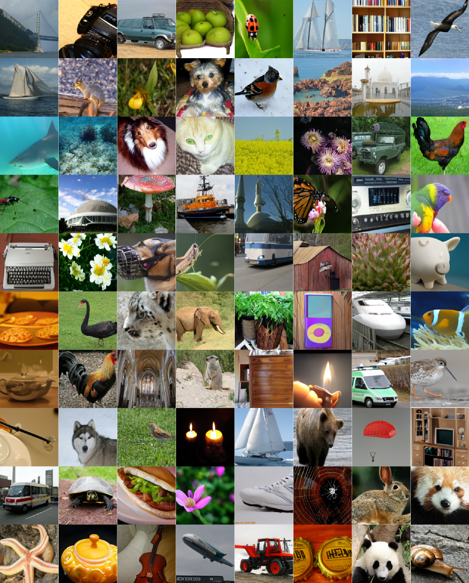
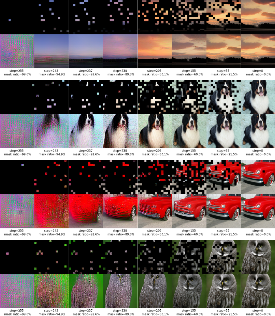
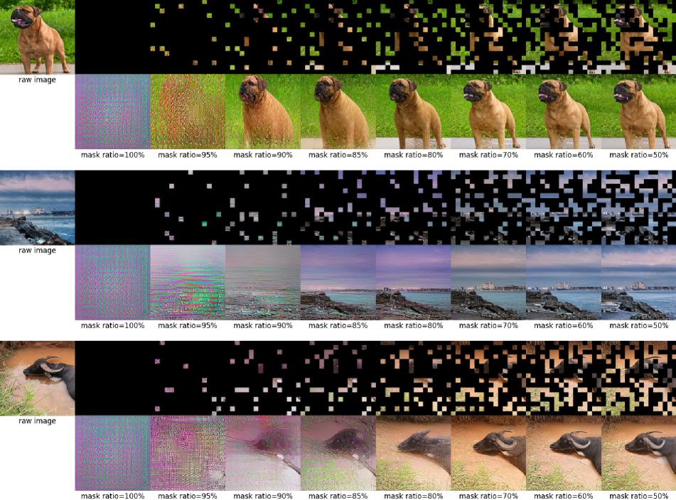
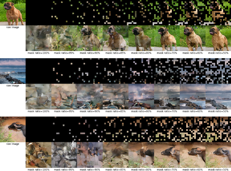
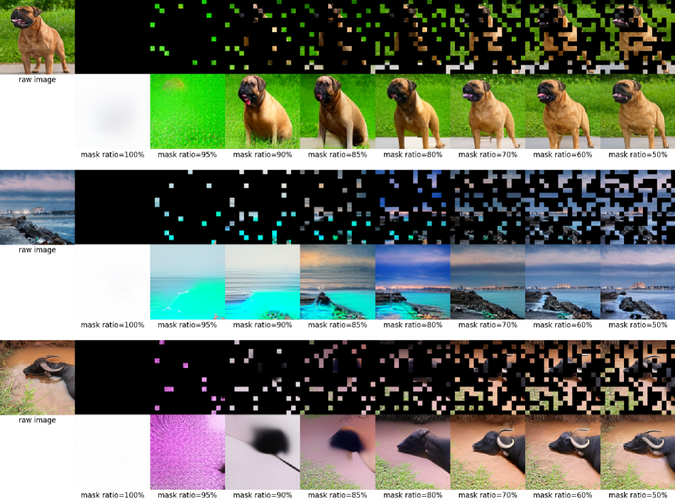
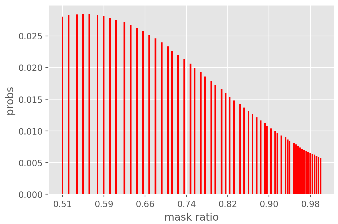
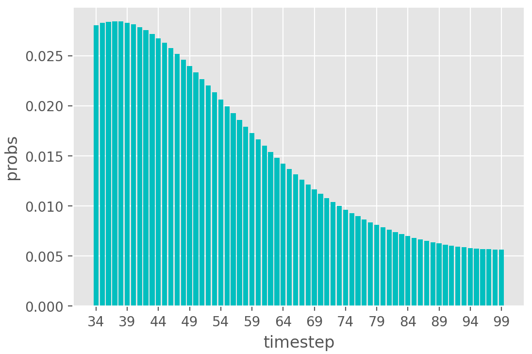
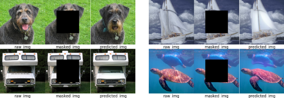
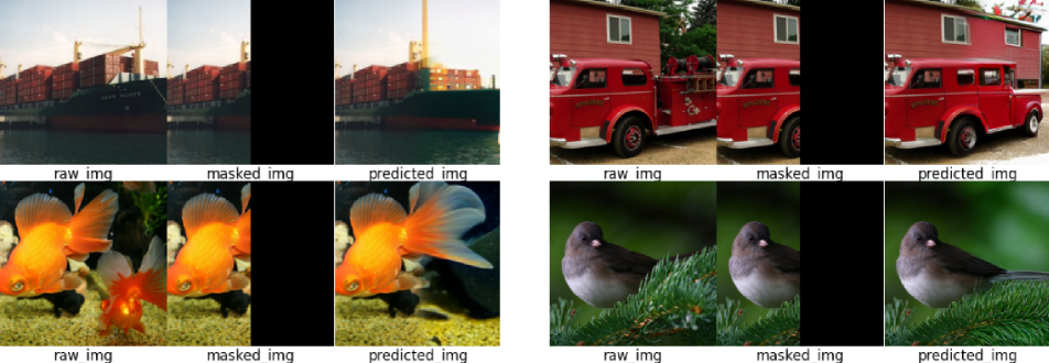
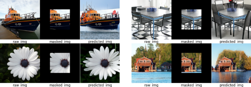
Image Inpainting and Outpainting.  ADDP is able to conduct image inpainting and outpainting without further finetuning. Given a masked image, we first generate the initial image $x_{t}$ by filling the masked region with the average pixels of visible areas. Then the mask ratio and the corresponding timestep $t$ is calculated based on the ratio of the masked area to the entire image. We also use VQ tokenizer to encode $x_{t}$ into VQ tokens $z_{t}$. After that, ADDP can generate the final image by continuing the subsequent alternating denoising process. The final output is composited with the input image via linear blending based on the mask, following MaskGIT [7]. Some results of image inpainting, outpainting and uncropping (outpainting on a large mask) are shown in Fig. 12, Fig. 13 and Fig. 14.

Figure 12: Results of image inpainting.

Figure 13: Results of image outpainting.

Figure 14: Results of image uncropping (outpainting on a large mask).

* ieee_fullname appendix_bib

References

- [1] Martin Arjovsky, Soumith Chintala, and Léon Bottou. Wasserstein Generative Adversarial Networks. In ICML, 2017.
- [2] Hangbo Bao, Li Dong, Songhao Piao, and Furu Wei. BEiT: BERT Pre-Training of Image Transformers. In ICLR, 2022.
- [3] Andrew Brock, Jeff Donahue, and Karen Simonyan. Large Scale GAN Training for High Fidelity Natural Image Synthesis. In ICLR, 2019.
- [4] Mathilde Caron, Hugo Touvron, Ishan Misra, Hervé Jégou, Julien Mairal, Piotr Bojanowski, and Armand Joulin. Emerging properties in self-supervised vision transformers. In ICCV, 2021.
- [5] Arantxa Casanova, Marlene Careil, Jakob Verbeek, Michal Drozdzal, and Adriana Romero Soriano. Instance-conditioned gan. NeurIPS, 2021.
- [6] Huiwen Chang, Han Zhang, Jarred Barber, AJ Maschinot, Jose Lezama, Lu Jiang, Ming-Hsuan Yang, Kevin Murphy, William T. Freeman, Michael Rubinstein, Yuanzhen Li, and Dilip Krishnan. Muse: Text-To-Image Generation via Masked Generative Transformers. arXiv preprint arXiv:2301.00704, 2023.
- [7] Huiwen Chang, Han Zhang, Lu Jiang, Ce Liu, and William T. Freeman. MaskGIT: Masked Generative Image Transformer. In CVPR, 2022.
- [8] Mark Chen, Alec Radford, Rewon Child, Jeff Wu, Heewoo Jun, David Luan, and Ilya Sutskever. Generative Pretraining from Pixels. In ICML, 2020.
- [9] Ting Chen, Simon Kornblith, Mohammad Norouzi, and Geoffrey Hinton. A Simple Framework for Contrastive Learning of Visual Representations. In ICML, 2020.
- [10] Xiaokang Chen, Mingyu Ding, Xiaodi Wang, Ying Xin, Shentong Mo, Yunhao Wang, Shumin Han, Ping Luo, Gang Zeng, and Jingdong Wang. Context Autoencoder for Self-Supervised Representation Learning. arXiv preprint arXiv:2202.03026, 2022.
- [11] Xi Chen, Yan Duan, Rein Houthooft, John Schulman, Ilya Sutskever, and Pieter Abbeel. InfoGAN: Interpretable Representation Learning by Information Maximizing Generative Adversarial Nets. In NeurIPS, 2016.
- [12] Xinlei Chen, Haoqi Fan, Ross Girshick, and Kaiming He. Improved Baselines with Momentum Contrastive Learning. arXiv preprint arXiv:2003.04297, 2020.
- [13] Xinlei Chen, Saining Xie, and Kaiming He. An Empirical Study of Training Self-Supervised Vision Transformers. In ICCV, 2021.
- [14] Jia Deng, Wei Dong, Richard Socher, Li-Jia Li, Kai Li, and Li Fei-Fei. Imagenet: A large-scale hierarchical image database. In CVPR, 2009.
- [15] Emily Denton, Soumith Chintala, Arthur Szlam, and Rob Fergus. Deep Generative Image Models using a Laplacian Pyramid of Adversarial Networks. In NeurIPS, 2015.
- [16] Jacob Devlin, Ming-Wei Chang, Kenton Lee, and Kristina Toutanova. Bert: Pre-training of deep bidirectional transformers for language understanding. arXiv preprint arXiv:1810.04805, 2018.
- [17] Prafulla Dhariwal and Alex Nichol. Diffusion Models Beat GANs on Image Synthesis. In NeurIPS, 2021.
- [18] Jeff Donahue, Philipp Krähenbühl, and Trevor Darrell. Adversarial Feature Learning. In ICLR, 2017.
- [19] Jeff Donahue and Karen Simonyan. Large Scale Adversarial Representation Learning. In NeurIPS, 2019.
- [20] Xiaoyi Dong, Jianmin Bao, Ting Zhang, Dongdong Chen, Weiming Zhang, Lu Yuan, Dong Chen, Fang Wen, Nenghai Yu, and Baining Guo. PeCo: Perceptual Codebook for BERT Pre-training of Vision Transformers. In AAAI, 2023.
- [21] Alexey Dosovitskiy, Lucas Beyer, Alexander Kolesnikov, Dirk Weissenborn, Xiaohua Zhai, Thomas Unterthiner, Mostafa Dehghani, Matthias Minderer, Georg Heigold, Sylvain Gelly, Jakob Uszkoreit, and Neil Houlsby. An Image is Worth 16x16 Words: Transformers for Image Recognition at Scale. In CVPR, 2021.
- [22] Patrick Esser, Robin Rombach, and Bjorn Ommer. Taming Transformers for High-Resolution Image Synthesis. In CVPR, 2021.
- [23] Yuxin Fang, Li Dong, Hangbo Bao, Xinggang Wang, and Furu Wei. Corrupted Image Modeling for Self-Supervised Visual Pre-Training. In ICLR, 2023.
- [24] Ian J. Goodfellow, Jean Pouget-Abadie, Mehdi Mirza, Bing Xu, David Warde-Farley, Sherjil Ozair, Aaron Courville, and Yoshua Bengio. Generative Adversarial Nets. In NeurIPS, 2014.
- [25] Shuyang Gu, Dong Chen, Jianmin Bao, Fang Wen, Bo Zhang, Dongdong Chen, Lu Yuan, and Baining Guo. Vector quantized diffusion model for text-to-image synthesis. In CVPR, 2022.
- [26] Kaiming He, Xinlei Chen, Saining Xie, Yanghao Li, Piotr Dollar, and Ross Girshick. Masked Autoencoders Are Scalable Vision Learners. In CVPR, 2022.
- [27] Kaiming He, Haoqi Fan, Yuxin Wu, Saining Xie, and Ross Girshick. Momentum Contrast for Unsupervised Visual Representation Learning. In CVPR, 2020.
- [28] Kaiming He, Xiangyu Zhang, Shaoqing Ren, and Jian Sun. Deep residual learning for image recognition. In CVPR, 2016.
- [29] Martin Heusel, Hubert Ramsauer, Thomas Unterthiner, Bernhard Nessler, and Sepp Hochreiter. Gans trained by a two time-scale update rule converge to a local nash equilibrium. NeurIPS, 2017.
- [30] Irina Higgins, Loic Matthey, Arka Pal, Christopher Burgess, Xavier Glorot, Matthew Botvinick, Shakir Mohamed, and Alexander Lerchner. -VAE: Learning Basic Visual Concepts with a Constrained Variational Framework. In ICLR, 2017.
- [31] Jonathan Ho, Ajay Jain, and Pieter Abbeel. Denoising diffusion probabilistic models. In NeurIPS, 2020.
- [32] Jeremy Howard and Sebastian Ruder. Universal language model fine-tuning for text classification. arXiv preprint arXiv:1801.06146, 2018.
- [33] Tero Karras, Timo Aila, Samuli Laine, and Jaakko Lehtinen. Progressive Growing of GANs for Improved Quality, Stability, and Variation. In ICLR, 2018.
- [34] Bahjat Kawar, Michael Elad, Stefano Ermon, and Jiaming Song. Denoising Diffusion Restoration Models. In NeurIPS, 2022.
- [35] Bahjat Kawar, Shiran Zada, Oran Lang, Omer Tov, Huiwen Chang, Tali Dekel, Inbar Mosseri, and Michal Irani. Imagic: Text-Based Real Image Editing with Diffusion Models. arXiv preprint arXiv:2210.09726, 2022.
- [36] Diederik P. Kingma and Max Welling. Auto-Encoding Variational Bayes. In ICLR, 2014.
- [37] Vladimir Kulikov, Shahar Yadin, Matan Kleiner, and Tomer Michaeli. SinDDM: A Single Image Denoising Diffusion Model. arXiv preprint arXiv:2211.16582, 2022.
- [38] Tianhong Li, Huiwen Chang, Shlok Kumar Mishra, Han Zhang, Dina Katabi, and Dilip Krishnan. Mage: Masked generative encoder to unify representation learning and image synthesis. arXiv preprint arXiv:2211.09117, 2022.
- [39] Tsung-Yi Lin, Michael Maire, Serge Belongie, James Hays, Pietro Perona, Deva Ramanan, Piotr Dollár, and C Lawrence Zitnick. Microsoft coco: Common objects in context. In ECCV, 2014.
- [40] Hao Liu, Xinghua Jiang, Xin Li, Antai Guo, Deqiang Jiang, and Bo Ren. The Devil is in the Frequency: Geminated Gestalt Autoencoder for Self-Supervised Visual Pre-Training. arXiv preprint arXiv:2204.08227, 2022.
- [41] Ze Liu, Yutong Lin, Yue Cao, Han Hu, Yixuan Wei, Zheng Zhang, Stephen Lin, and Baining Guo. Swin transformer: Hierarchical vision transformer using shifted windows. In ICCV, 2021.
- [42] Ilya Loshchilov and Frank Hutter. Decoupled weight decay regularization. arXiv preprint arXiv:1711.05101, 2017.
- [43] Mehdi Mirza and Simon Osindero. Conditional Generative Adversarial Nets. arXiv preprint arXiv:1411.1784, 2014.
- [44] Zhiliang Peng, Li Dong, Hangbo Bao, Qixiang Ye, and Furu Wei. BEiT v2: Masked Image Modeling with Vector-Quantized Visual Tokenizers. arXiv preprint arXiv:2208.06366, 2022.
- [45] Alec Radford, Luke Metz, and Soumith Chintala. Unsupervised Representation Learning With Deep Convolutional Generative Adversarial Networks. In ICLR, 2016.
- [46] Alec Radford, Karthik Narasimhan, Tim Salimans, Ilya Sutskever, et al. Improving language understanding by generative pre-training. 2018.
- [47] Aditya Ramesh, Prafulla Dhariwal, Alex Nichol, Casey Chu, and Mark Chen. Hierarchical Text-Conditional Image Generation with CLIP Latents. arXiv preprint arXiv:2204.06125, 2022.
- [48] Ali Razavi, Aaron van den Oord, and Oriol Vinyals. Generating Diverse High-Fidelity Images with VQ-VAE-2. In NeurIPS, 2019.
- [49] Robin Rombach, Andreas Blattmann, Dominik Lorenz, Patrick Esser, and Bjorn Ommer. High-Resolution Image Synthesis with Latent Diffusion Models. In CVPR, 2022.
- [50] Chitwan Saharia, William Chan, Saurabh Saxena, Lala Li, Jay Whang, Emily Denton, Seyed Kamyar Seyed Ghasemipour, Burcu Karagol Ayan, S. Sara Mahdavi, Rapha Gontijo Lopes, Tim Salimans, Jonathan Ho, David J Fleet, and Mohammad Norouzi. Photorealistic Text-to-Image Diffusion Models with Deep Language Understanding. In NeurIPS, 2022.
- [51] Tim Salimans, Ian Goodfellow, Wojciech Zaremba, Vicki Cheung, Alec Radford, and Xi Chen. Improved techniques for training gans. NeurIPS, 2016.
- [52] Tim Salimans, Andrej Karpathy, Xi Chen, and Diederik P. Kingma. PixelCNN++: Improving the PixelCNN with Discretized Logistic Mixture Likelihood and Other Modifications. In ICLR, 2017.
- [53] Chenxin Tao, Xizhou Zhu, Weijie Su, Gao Huang, Bin Li, Jie Zhou, Yu Qiao, Xiaogang Wang, and Jifeng Dai. Siamese Image Modeling for Self-Supervised Vision Representation Learning. In CVPR, 2023.
- [54] Arash Vahdat and Jan Kautz. NVAE- A Deep Hierarchical Variational Autoencoder. In NeurIPS, 2020.
- [55] Aäron van den Oord, Nal Kalchbrenner, and Koray Kavukcuoglu. Pixel Recurrent Neural Networks. In ICML, 2016.
- [56] Aäron van den Oord, Nal Kalchbrenner, Oriol Vinyals, Lasse Espeholt, Alex Graves, and Koray Kavukcuoglu. Conditional Image Generation with PixelCNN Decoders. In NeurIPS, 2016.
- [57] Aaron van den Oord, Oriol Vinyals, and Koray Kavukcuoglu. Neural Discrete Representation Learning. In NeurIPS, 2017.
- [58] Ashish Vaswani, Noam Shazeer, Niki Parmar, Jakob Uszkoreit, Llion Jones, Aidan N Gomez, Ł ukasz Kaiser, and Illia Polosukhin. Attention is all you need. In NeurIPS, 2017.
- [59] Chen Wei, Haoqi Fan, Saining Xie, Chao-Yuan Wu, Alan Yuille, and Christoph Feichtenhofer. Masked Feature Prediction for Self-Supervised Visual Pre-Training. In CVPR, 2022.
- [60] Jiahui Yu, Xin Li, Jing Yu Koh, Han Zhang, Ruoming Pang, James Qin, Alexander Ku, Yuanzhong Xu, Jason Baldridge, and Yonghui Wu. Vector-quantized image modeling with improved VQGAN. In ICLR, 2021.
- [61] Han Zhang, Ian Goodfellow, Dimitris Metaxas, and Augustus Odena. Self-Attention Generative Adversarial Networks. In ICML, 2019.
- [62] Zhixing Zhang, Ligong Han, Arnab Ghosh, Dimitris Metaxas, and Jian Ren. SINE: SINgle Image Editing with Text-to-Image Diffusion Models. arXiv preprint arXiv:2212.04489, 2022.
- [63] Bolei Zhou, Hang Zhao, Xavier Puig, Tete Xiao, Sanja Fidler, Adela Barriuso, and Antonio Torralba. Semantic understanding of scenes through the ade20k dataset. IJCV, 2019.
- [64] Jinghao Zhou, Chen Wei, Huiyu Wang, Wei Shen, Cihang Xie, Alan Yuille, and Tao Kong. Image bert pre-training with online tokenizer. In ICLR, 2022.
- [65] Jun-Yan Zhu, Taesung Park, Phillip Isola, and Alexei A. Efros. Unpaired Image-to-Image Translation using Cycle-Consistent Adversarial Networks. In ICML, 2017.