The FRB20190520B Sightline Intersects Foreground Galaxy Clusters

Abstract

The repeating fast radio burst FRB20190520B is an anomaly of the FRB population thanks to its high dispersion measure (DM$=1205\,\rm pc\,cm^{-3}$) despite its low redshift of $z_{\mathrm{frb}}=0.241$. This excess has been attributed to a large host contribution of $\mathrm{DM}_{\mathrm{host}}\approx 900\,\rm pc\,cm^{-3}$, far larger than any other known FRB. In this paper, we describe spectroscopic observations of the FRB20190520B field obtained as part of the FLIMFLAM survey, which yielded 701 galaxy redshifts in the field. We find multiple foreground galaxy groups and clusters, for which we then estimated halo masses by comparing their richness with numerical simulations. We discover two separate $M_{\mathrm{halo}}>10^{14}\,M_{\odot}$ galaxy clusters, at $z=0.1867$ and $z=0.2170$, respectively, that are directly intersected by the FRB sightline within their characteristic halo radius $r_{200}$. Subtracting off their estimated DM contributions as well that of the diffuse intergalactic medium, we estimate a host contribution of $\mathrm{DM}_{\mathrm{host}}=430^{+140}_{-220}\,\rm pc\,cm^{-3}$ or $\mathrm{DM}_{\mathrm{host}}=280^{+140}_{-170}\,\rm pc\,cm^{-3}$ (observed frame) depending on whether we assume the halo gas extends to $r_{200}$ or $2\times r_{200}$. This significantly smaller $\mathrm{DM}_{\mathrm{host}}$ — no longer the largest known value — is now consistent with H$\alpha$ emission measures of the host galaxy without invoking unusually high gas temperatures. Combined with the observed FRB scattering timescale, we estimate the turbulent fluctuation and geometric amplification factor of the scattering layer to be $\widetilde{F}G\approx 4.5-11\,(\mathrm{pc^{2}\;km})^{-1/3}$, suggesting most of the gas is close to the FRB host. This result illustrates the importance of incorporating foreground data for FRB analyses, both for understanding the nature of FRBs and to realize their potential as a cosmological probe.

1 Introduction

Fast radio bursts (FRBs) are phenomena that have excited tremendous interest, not just because of the enigmatic nature of their source engines, but also because their frequency sweeps encode information on the integrated free electron column density along their lines-of-sight. This is usually quantified through the dispersion measure, $\mathrm{DM}=\int n_{e}(l)\,\mathrm{d}l$, where $n_{e}(l)$ is the free electron density along the line-of-sight path $l$.

Among the sample of FRBs that have been localized at the time of writing, FRB20190520B ranks among the most notable. First reported by Niu et al. (2022), it was discovered as a sequence of repeating bursts by the Five-Hundred Aperture Spherical Radio Telescope (FAST; Nan et al., 2011; Li et al., 2018) that was subsequently localized with the Karl. G. Jansky Very Large Array (VLA; Law et al., 2018) to the Equatorial J2000 coordinates (RA, Dec)=(16:02:04.261, -11:17:17.35). Follow-up optical imaging and spectroscopy revealed a host galaxy, J160204.31-111718.5 (hereafter referred to as HG190520), that was associated with the FRB at high confidence. This galaxy was measured to have a spectroscopic redshift of $z_{\mathrm{frb}}=0.241$, and also has an associated persistent radio source.

With a total measured dispersion measure of $\mathrm{DM}_{\mathrm{FRB}}=1204.7\pm 4.0\,\rm pc\,cm^{-3}$ (Niu et al., 2022), FRB20190520B has a DM well in excess of the value expected given its redshift and the Macquart Relation (Macquart et al., 2020): assuming a Milky Way contribution of ${\rm DM}_{\rm MW}\sim 100\,\rm pc\,cm^{-3}$ and a mean IGM contribution of $\langle{\rm DM}_{\rm IGM}\rangle\sim 300\,\rm pc\,cm^{-3}$ (using the rough approximations of Ioka 2003 and Inoue 2004), FRB20190520B exhibits a DM over twice that expected given its redshift. This was attributed to a large host contribution of $\mathrm{DM}_{\mathrm{host}}=903^{+72}_{-111}\,\rm pc\,cm^{-3}$ (observed frame; Niu et al. 2022), which makes it by far the largest host DM value of any known FRB prior to this current analysis.

While Niu et al. (2022) and Ocker et al. (2022) concluded that no foreground galaxies were likely to contribute to the foreground DM, they based this conclusion on a single pointing of Keck/LRIS observations which was limited to $\sim 2-3\arcmin$ from the FRB sightline. This would be adequate to reveal, for example, the influence of a foreground galaxy at $z=0.15$ with a halo mass $M_{\mathrm{halo}}\sim 10^{12}\,M_{\odot}$ since its characteristic radius of $r_{200}\approx 240\,\mathrm{pkpc}$ would extend 1.5$\arcmin$. However, a modestly more massive foreground halo with, say, $M_{\mathrm{halo}}\sim 3\times 10^{13}\,M_{\odot}$, at the same redshift would have a $r_{200}$ extending to $4.7\arcmin$ from the halo center. This would be outside the field of the original optical observations, and would require wide field-of-view multiplexed spectroscopy to characterize the multiple member galaxies. Wider observations than originally achieved in the discovery papers are therefore needed to rule out significant foreground contributions to the large DM of FRB20190520B.

In this paper, we describe wide-field multiplexed spectroscopic data we have obtained in the FRB20190520B field as part of the FRB Line-of-sight Ionization Measurement From Lightcone AAOmega Mapping (FLIMFLAM) Survey (Lee et al., 2022). This survey, which is carried out on the 2dF/AAOmega fiber spectrograph on the 3.9m Anglo-Australian Telescope (AAT) in Siding Spring, Australia, is designed to observed large numbers of galaxy redshifts in the foregrounds of localized FRBs in order to map the large-scale structure in the foreground. As shown by Simha et al. (2020), this would allow us to separate the various components that make up the DM observed in FRBs. We then describe the group-finding approach applied to the spectroscopic data using a commonly-used friends-of-friends (FoF) algorithm to identify galaxy groups and clusters within the FRB20190520B field. The group/cluster halo masses are then estimated by comparing with forward models of group/cluster richness derived from cosmological $N$-body simulations. Next, we model the implied DM from both the foreground halos and diffuse IGM, yielding updated estimates for the FRB20190520B DM host contribution. Finally, we discuss the implications of the new host estimate in context of the observed host galaxy H$\alpha$ emission and FRB scattering. In a separate paper, Simha et al. (2023) had analyzed 4 other sightlines also shown to exhibit an excess $\mathrm{DM}_{\mathrm{FRB}}$ given their redshift, but FRB20190520B was deemed such an unusual object that it merited a separate analysis and paper.

In this paper, we use the term ‘groups’ to refer to both groups and clusters when we are agnostic as to their underlying halo masses, but use ‘cluster’ to refer specifically to objects with $M_{\mathrm{halo}}\geq 10^{14}\,M_{\odot}$. We use a concordance $\Lambda$CDM cosmology with $\sigma_{8}=0.829$, $H_{0}=67.3\,\mathrm{km}\,\mathrm{s}^{-1}\mathrm{Mpc}^{-1}$, $h=H_{0}/(100\,\mathrm{km}\,\mathrm{s}^{-1}\mathrm{Mpc}^{-1})=0.673$, $\Omega_{\Lambda}=0.685$, $\Omega_{m}=0.315$, $\Omega_{b}=0.0487$, and $n=0.96$.

2 Observations

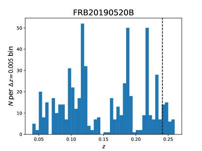
Figure 1: The galaxy redshift distribution from our AAT/2dF-AAOmega spectroscopic observations, which targeted an approximately 2 degree field of view centered on FRB20190520B. The FRB redshift ($z_{\mathrm{frb}}=0.241$) is indicated by the vertical-dashed line.

In order to characterize the foreground contributions to the FRB20190520B dispersion measure (DM), we carried out a sequence of observations as part of the broader FLIMFLAM survey (Lee et al., 2022). Since FRB20190520B was immediately reported to have an anomalously high $\mathrm{DM}_{\mathrm{host}}$ by Niu et al. (2022), it was deemed to be of sufficient scientific interest to constrain the foreground contributions of FRB20190520B, and therefore it was added to the FLIMFLAM observation list as a special target.

FRB20190520B was not, to our knowledge, within the footprint of publicly-available imaging surveys, therefore on 2021 August 8 we imaged the field with a single pointing of the Dark Energy Camera (DECam) in $r$-band. The data was then reduced using the standard pipeline provided by the observatory, and a galaxy catalog generated using SourceExtractor (Bertin & Arnouts, 1996) after excluding point sources as stars. Since the DECam imaging preceded the spectroscopic run with AAT/AAOmega by only one month, at the time of spectroscopic target selection we had only preliminary image reductions that did not have a well-characterized magnitude zero-point. For the spectroscopic target selection, we therefore defined an arbitrary magnitude cut in the $r$-band to select approximately 1500 targets within the 2 degree diameter (i.e. 3.14 deg²) footprint of AAT/AAOmega. This was intended to target an areal density of galaxies that should, on average, correspond approximately to a magnitude limit of $r\approx 19.4$ mag, which is our magnitude limit for FRBs at $z\approx 0.2$ (c.f. Simha et al. 2023). However, this selection was later found to actually correspond to an apparent depth of $r=19.1$ mag or unextincted magnitude of $r_{\mathrm{dered}}=18.4$ mag based on corrections using the Schlafly & Finkbeiner (2011) dust map. This field is thus overdense in galaxies given the relative shallowness of the magnitude threshold, as we shall see later. We note that there is significant variation ($\sim 0.4$ mag) in the extinction across our 3.1 deg² field which makes it challenging to compare the number counts with simulations, but our forward model described later should be accurate in the vicinity of the FRB position.

Using configure (Miszalski et al., 2006), the standard plate configuration software provided by the observatory, we designed 5 plates filled with approximately 300 galaxies each across the 3.1 sq deg 2dF footprint, of which 3 were observed with AAOmega on UT 2021 Sept 7-9. The observing setup was the 580V grating blazed at 485nm on the blue camera, while the red camera used the 385R grating blazed at 720nm. In combination with the 570nm dichroic, this allowed a continuous spectral coverage across 380nm-880nm with a spectral resolving power of $R\approx 1300$. Each plate received 4500s-5400s of on-sky exposure; the first plate was observed in sub-optimal seeing of $3-3.5\arcsec$ on 2021 Sept 7, but the subsequent two plates were observed under nominal conditions in the following nights with $1.6-1.8\arcsec$ seeing.

The raw data was reduced using a version of the 2dFDR data reduction package kindly provided by the OzDES collaboration (Yuan et al., 2015; Childress et al., 2017). We then ran the MARZ software (Hinton et al., 2016) on the spectra to measure spectroscopic redshifts, which were then visually confirmed. Redshift identifications that appeared to be a reasonable match to the spectral templates were assigned a quality operator (QOP) flag of 3, while high-confidence redshifts with multiple high signal-to-noise features were assigned QOP$=4$. There were 701 galaxies that had QOP$=(3\lor 4)$, which we consider to be ‘successful’ redshifts and will treat identically in the subsequent analysis. The galaxy redshift histogram is shown in Figure 1, which shows distinct redshift peaks that are suggestive of overdensities within the field. This motivates us to apply group-finding algorithms to search for galaxy groups or clusters within the sample.

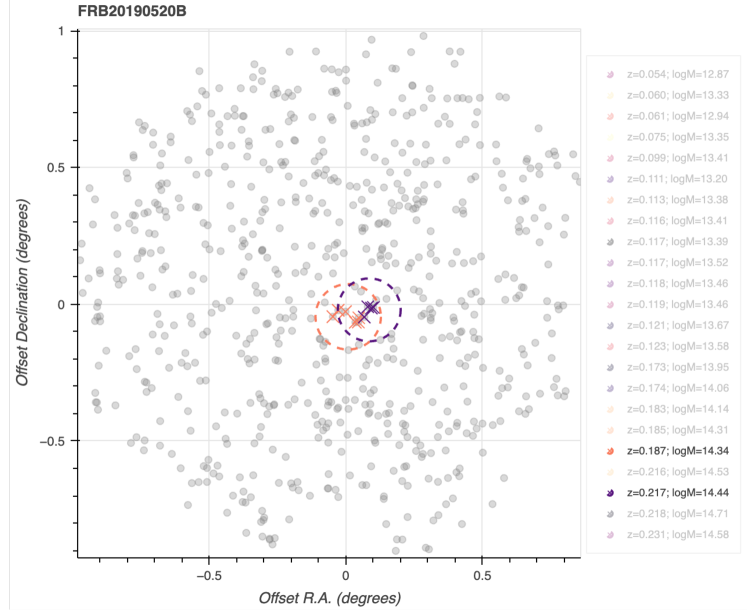
Figure 2: Preview of an interactive visualization of the FLIMFLAM foreground redshifts in the FRB20190520B field (click on this URL for full version). The gray points indicate galaxies with measured spectroscopic redshifts, with their positions on the sky shown as a relative angular offset from the FRB20190520B coordinate (i.e. the FRB is at [0,0]). In the online version, pan-dragging and zooming is supported (tool bar on top), while hovering over an individual galaxy with the mouse will show the coordinate and redshift. Clicking on the legend on the right will highlight galaxy groups labeled by redshift, with group members marked with ’$\times$’ and the physical extent of $r_{200}$ indicated by a dashed circle. In the static preview, we have highlighted the clusters at $z_{\mathrm{grp}}=0.1867$ and $z_{\mathrm{grp}}=0.2170$ that are believed to provide large contributions to $\mathrm{DM}_{\mathrm{halos}}$. Full version will be available in the online published journal.

During visual inspection of the spectra, we found 122 confirmed stars compared to 701 galaxies, or a stellar contamination rate of 17.4%. This is relatively high compared to the other fields observed by FLIMFLAM, presumably due to the low Galactic latitude ($b=29$ deg) and imperfect star-galaxy separation. If we assume that the stellar contamination rate is same between the spectroscopically confirmed targets and those that could not be assigned a conclusive redshift, then the spectroscopic completeness success rate of our galaxy sample is 701 out of 1260 possible galaxy targets, or 56.6%.

3 Halos

We applied an anisotropic friends-of-friends (FoF) group-finding algorithm on our FRB20190520B spectroscopic data, kindly provided by Elmo Tempel (Tago et al., 2008; Tempel et al., 2012, 2014). While standard FoF algorithms, such as those used to identify dark matter halos in $N$-body simulations, typically adopt the same linking length in all 3 dimensions, Tempel’s code allows for a longer linking length in the radial dimension in order to account for redshift-space distortions, i.e. the “Fingers of God”.

This finder assumes a transverse linking length, $d_{\mathrm{LL,\perp}}$, which varies as a function of redshift, $z$, in the following way:

$$d_{\mathrm{LL,\perp}}(z)=d_{\mathrm{LL,0}}[1+a\,\mathrm{arctan}(z/z_{*})],$$ (1)

where $d_{\mathrm{LL,0}}$ is the linking length at a fiducial redshift, while $a$ and $z_{*}$ govern the redshift evolution. This redshift dependence accounts for the artificial decreasing number of galaxies as a function of redshift, within a flux-limited survey. We then set the radial linking length, $d_{\mathrm{LL,\parallel}}(z)$, to be proportional to $d_{\mathrm{LL,\perp}}(z)$. The final parameters used for group-finding in this paper are: $d_{\mathrm{LL,\perp}}=0.35\,h^{-1}\,\mathrm{Mpc}$, $a=0.75$, $z_{*}=0.1$, and $d_{\mathrm{LL,\parallel}}/d_{\mathrm{LL,\perp}}=10$. Note that we adopt a linking length which is larger than used in Simha et al. (2023) in order to account for our sparser sample of redshifts, which is nearly a factor of two lower space density than in Simha et al. (2023).

The resulting group catalog has groups with richness or multiplicity (i.e. number of identified galaxies) as low as $N_{\mathrm{rich}}=2$, but we limit ourselves to $N_{\mathrm{rich}}=4$ to have a more robust sample. These are listed in Table 1, although note that we omit groups with $z_{\mathrm{grp}}>z_{\mathrm{frb}}$. We do not find any group with $z_{\mathrm{grp}}\approx z_{\mathrm{frb}}$, which can be plausibly associated with the FRB host.

In Figure  2, we present an interactive plot that shows the position of the galaxies as well as identified groups within the FRB field.

Table 1: Detected Galaxy Groups and Clusters in the FRB20190520B Field.

ID	$z_{\mathrm{grp}}$	RA	Dec	$b_{\perp}$	$b_{\perp}$	$N_{\mathrm{rich}}$	$\log_{10}\!\left(\frac{M_{\mathrm{halo}}}{M_{\odot}}\right)$	$r_{200}$	$b_{\perp}$
		(deg)	(deg)	(arcmin)	(kpc)			(kpc)	($r_{200}$)
2403390701118753	0.0536	240.3391	-11.1875	12.13	789.1	4	$12.87^{+0.21}_{-0.90}$	453	1.74
2400721001053090	0.0605	240.0721	-10.5309	52.48	3820.3	7	$13.33^{+0.10}_{-0.10}$	644	5.93
2407627701151079	0.0608	240.7628	-11.5108	19.65	1437.7	4	$12.94^{+0.28}_{-0.23}$	478	3.01
2402176201159096	0.0745	240.2176	-11.5910	25.33	2236.3	6	$13.35^{+0.15}_{-0.28}$	654	3.42
2399925001187499	0.0991	239.9925	-11.8750	46.83	5342.0	5	$13.41^{+0.16}_{-0.46}$	685	7.80
2404259001164001	0.1114	240.4259	-11.6400	21.79	2753.9	4	$13.20^{+0.34}_{-0.37}$	583	4.72
2404782701043103	0.1133	240.4783	-10.4310	51.48	6602.6	4	$13.38^{+0.23}_{-0.58}$	670	9.86
2401932701109639	0.1163	240.1933	-11.0964	22.30	2925.7	4	$13.41^{+0.25}_{-0.59}$	685	4.27
2395862301164344	0.1166	239.5862	-11.6434	58.78	7728.4	4	$13.39^{+0.25}_{-0.56}$	675	11.45
2404329301079377	0.1169	240.4329	-10.7938	30.08	3965.7	5	$13.52^{+0.19}_{-0.43}$	746	5.32
2405894601098030	0.1176	240.5895	-10.9803	18.95	2509.3	4	$13.46^{+0.21}_{-0.63}$	712	3.52
2406789301111492	0.1189	240.6789	-11.1149	14.07	1881.9	4	$13.46^{+0.21}_{-0.58}$	712	2.64
2409852201173268	0.1211	240.9852	-11.7327	38.30	5203.4	6	$13.67^{+0.17}_{-0.30}$	836	6.22
2408283601132797	0.1228	240.8284	-11.3280	18.43	2533.4	5	$13.58^{+0.20}_{-0.48}$	781	3.25
2408321001051411	0.1727	240.8321	-10.5141	50.00	9140.7	4	$13.95^{+0.23}_{-0.47}$	1037	8.81
2411417701121786	0.1741	241.1418	-11.2179	36.96	6803.0	5	$14.06^{+0.20}_{-0.30}$	1128	6.03
2402401701215090	0.1833	240.2402	-12.1509	54.27	10409.6	4	$14.14^{+0.19}_{-0.83}$	1200	8.68
2405098001170259	0.1851	240.5098	-11.7026	24.87	4807.9	6	$14.31^{+0.19}_{-0.30}$	1367	3.52
2405265701133378	0.1867	240.5266	-11.3338	2.79	542.4	6	$14.34^{+0.18}_{-0.28}$	1399	0.39
2401408901101955	0.2164	240.1409	-11.0195	27.42	5989.1	5	$14.53^{+0.19}_{-0.31}$	1619	3.70
2406051301130845	0.2170	240.6051	-11.3084	5.28	1155.5	4	$14.44^{+0.20}_{-0.40}$	1511	0.76
2407679601092642	0.2175	240.7680	-10.9264	26.23	5750.6	7	$14.71^{+0.18}_{-0.25}$	1858	3.09
2405885701164888	0.2315	240.5886	-11.6489	22.04	5065.3	4	$14.58^{+0.22}_{-0.43}$	1682	3.01

3.1 Estimating Group/Cluster Masses

In Simha et al. (2023), we adopted dynamical halo masses estimated using the virial theorem applied to the projected size and velocity dispersion of the galaxy groups. For the foreground sample of FRB20190520B, however, the observations were much shallower and the spectroscopic success rate was considerably lower than equivalent datasets in Simha et al. (2023). For example, Simha et al. (2023) had 1493 galaxy redshifts for the FRB20190714A field which is at $z_{\mathrm{frb}}=0.2365$, whereas for FRB20190520B at the similar redshift of $z_{\mathrm{frb}}=0.241$ we only have 701 successful galaxy redshifts. We therefore consider the FRB20190520B sample too sparse for reliable application of the virial theorem for group/cluster mass estimation.

Instead, we use the group richness, $N_{\mathrm{rich}}$, combined with a forward-modeling approach based on semi-analytic models of galaxy formation. Specifically, we use the Henriques et al. (2015) lightcone catalogs that were generated by applying the “Munich” semi-analytic galaxy formation model (Guo et al., 2011) to the $L=500\,h^{-1}\,\mathrm{Mpc}$ Millennium $N$-body simulation (Springel, 2005). In particular, we use the “all-sky” catalogs that are designed to simulate footprints covering $4\pi$ sr in order to maximize the number of simulated groups and clusters. We queried the simulation SQL database to download $z<0.25$ cluster catalogs with $\log_{10}(M_{\mathrm{halo}}/M_{\odot})\geq 14.2$ from over the full sky, whereas for the halo mass range $13.0\leq\log_{10}(M_{\mathrm{halo}}/M_{\odot})<14.2$ a subsample over a footprint of 400 deg² was deemed to provide a sufficient sample size to probe the diversity of the groups without having to download an excessively large file. This simulated group catalog includes effects such as $K$-corrected photometry based on the realistic galaxy spectral energy distributions (including the effect of dust), redshift space distortions, and the distance modulus (i.e. increasingly faint magnitudes as a function of redshift).

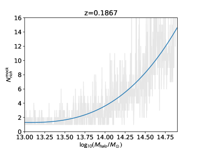
Figure 3: An example of our halo mass estimation model using the group richness, built from mock group/clusters from the Millennium simulation. The light grey curve show the richness of an ensemble of mock groups selected at the redshift of our detected group at $z_{\mathrm{grp}}=0.1867$, after incorporating the incompleteness and magnitude threshold of our data. The curve is the spline fit to this ensemble of mock groups, which is then used to estimate the halo masses as a function of the group richness.

Using these mock catalogs, we build forward models matched to the observed redshift, $z_{\mathrm{grp}}$, of each detected group in our sample. First, we selected groups/clusters from the mock catalog within $z_{\mathrm{grp}}\pm 0.005$, and applied the same magnitude cut as that corresponding to our field center, $r\leq 18.42$ (with a small distance modulus correction to account for the finite width of the $\Delta z=0.005$ redshift selection bin). This step yields $N^{\mathrm{true}}_{\mathrm{rich}}$ group members that would be observed within our observing setup if we had achieved 100% spectroscopic completeness. We then downsample each group to our actual observed completeness by drawing a random Poisson variate with a mean of $\mu=f_{\mathrm{obs}}\,N^{\mathrm{true}}_{\mathrm{rich}}$, where $f_{\mathrm{obs}}=56.6\%$ is the completeness of our FRB20190520B spectroscopy. The selected group galaxies are used to compute the observed mock richness, $N^{\mathrm{mock}}_{\mathrm{rich}}=\mu\,N^{\mathrm{true}}_{\mathrm{rich}}$, for that simulated group. In Figure 3, the gray lines show $N^{\mathrm{mock}}_{\mathrm{rich}}$ computed as a function of $\log_{10}(M_{\mathrm{halo}})$ for an ensemble of simulated groups selected to be at the same redshift as one of our observed groups. The scatter originates from both the intrinsic diversity of group properties at fixed halo mass, and also from the stochasticity induced by the Poisson sampling at our low spectroscopic completeness. We then fit a spline function to obtain $N^{\mathrm{mock}}_{\mathrm{rich}}$ as a function of $\log_{10}(M_{\mathrm{halo}})$. While there are gaps in the sample of mock groups at certain masses, especially at the massive end, the spline fit appears to be a reasonable model for $N^{\mathrm{mock}}_{\mathrm{rich}}$ as a function of $\log_{10}(M_{\mathrm{halo}})$.

To estimate the halo masses, we then use the standard Chi-squared minimization methodology:

$$\chi^{2}=\frac{(N_{\mathrm{rich}}-N^{\mathrm{mock}}_{\mathrm{rich}})^{2}}{\sigma_{N}^{2}},$$ (2)

where $\sigma_{N}=\sqrt{N_{\mathrm{rich}}}$ is the observational errors on $N_{\mathrm{rich}}$, which we estimate to be simply the Poisson uncertainty. We evaluate this on a grid of halo masses in the range $13.0<\log_{10}(M_{\mathrm{halo}}/M_{\odot})<14.9$ using the spline-fitted model for $N^{\mathrm{mock}}_{\mathrm{rich}}$ described above obtained for each redshift. The best-fit halo mass is given by the minimum $\chi^{2}$, while we also estimate the 68th percentile uncertainties by evaluating the halo masses at $\Delta\chi^{2}=1$. The estimated halo masses are listed in Table 1, along with the corresponding $r_{200}$, the characteristic halo radius within which the halo matter density is $200\times$ the mean density of the Universe at that redshift.

Notably, we find several foreground galaxy clusters with halo masses of $\log_{10}(M_{\mathrm{halo}}/M_{\odot})>14$. Two of these clusters are intersected by the FRB sightline within their characteristic cluster radius: (1) at $z_{\mathrm{grp}}=0.1867$, a galaxy cluster with $\log_{10}(M_{\mathrm{halo}}/M_{\odot})=14.34^{+0.18}_{-0.28}$ lies at a mere 2.79$\arcmin$ or $b_{\perp}=542\,\mathrm{pkpc}$ from the FRB sightline, which corresponds to 0.388$\times r_{200}$ and; (2) another, separate, cluster is at $z=0.2170$ with an estimated halo mass of $\log_{10}(M_{\mathrm{halo}}/M_{\odot})=14.44^{+0.20}_{-0.40}$, intersecting the sightline at 0.765$\times r_{200}$.

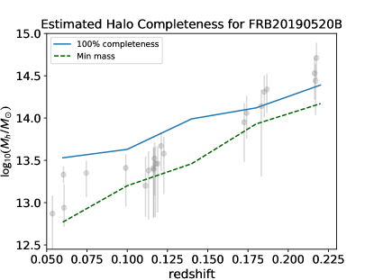
Figure 4: Data points show the redshift and estimated halo masses of the detected groups from our FRB20190520B spectroscopic data. Curves show the estimated mass completeness of simulated groups and clusters as a function of redshift, assuming the observational depth and completeness of our data. The dashed curve indicates the minimum mass at which groups are detectable with $N_{\mathrm{rich}}\geq 4$ at the given redshift, while the solid curve indicates the mass at which we expect to be 100% complete.

At first glance, it might appear that there are preferentially more low-mass groups at the low-redshift end of our spectroscopic data, while the more massive clusters lie preferentially toward the higher redshifts. However, this is a selection effect in that only more massive groups or clusters are detectable as multiple galaxy members with our relatively shallow magnitude threshold and low completeness. This is shown in Figure 4, in which we use the lightcone galaxy catalogs of Henriques et al. (2015) to derive the our expected completeness of $N_{\mathrm{rich}}\geq 4$ groups and clusters as a function of halo mass and redshift. This takes into account the estimated observational depth and incompleteness, as well as the intrinsic variance in the number of member galaxies for each halo mass. The masses that can be selected do indeed increase as a function of redshift, consistent with what we see in our data. While we are confident that we have ruled out massive clusters at $z<0.15$ in our field, we suspect that more complete spectroscopic observations would reveal multiple lower-mass groups associated with the clusters detected at $z>0.17$. Indeed, our detected clusters are not isolated, with multiple entities detected at similar redshifts — indicative of true overdensities and related structures in the cosmic web.

4 Analysis

In this paper, we adopt the observed DM value of $\mathrm{DM}_{\mathrm{FRB}}=(1205\pm 4)\,\rm pc\,cm^{-3}$ for FRB20190520B, as reported by Niu et al. (2022). We then decompose the total observed DM contribution for FRB20190520B into several components:

$$\mathrm{DM}_{\mathrm{FRB}}={\rm DM}_{\rm MW}+\mathrm{DM}_{\mathrm{halos}}+\mathrm{DM}_{\mathrm{IGM}}+\mathrm{DM}_{\mathrm{host}},$$ (3)

where ${\rm DM}_{\rm MW}$ is the contribution from the Milky Way, $\mathrm{DM}_{\mathrm{halos}}$ is the summed contribution from individual halos that intersect the sightline, $\mathrm{DM}_{\mathrm{IGM}}$ is the contribution from the diffuse intergalactic medium (IGM) outside of halos, and $\mathrm{DM}_{\mathrm{host}}$ is the combined contribution from the host galaxy and FRB engine. Note that the notation $\mathrm{DM}_{\mathrm{IGM}}$ is sometimes used to refer to the sum of $\mathrm{DM}_{\mathrm{halos}}$ and $\mathrm{DM}_{\mathrm{IGM}}$ in the literature, but in this paper we explicitly separate out the IGM and halo contributions. For the Milky Way component, we use the same estimate by Niu et al. (2022) of ${\rm DM}_{\rm MW}=113\,\rm pc\,cm^{-3}$ for the disk and halo contribution from the Milky Way, respectively. The disk contribution was estimated by averaging the NE2001 (Cordes & Lazio, 2002) and YMW16 (Yao et al., 2017) disk models. The Galactic halo contribution, on the other hand, was estimated using models from Prochaska & Zheng (2019), Ravi et al. (2023), and Cook et al. (2023).

In the following subsections, we will assess the contributions of $\mathrm{DM}_{\mathrm{halos}}$ and $\mathrm{DM}_{\mathrm{IGM}}$ based on our observational data.

4.1 Foreground Halo Contributions

We have now established that the FRB20190520B sightline directly intersects within $<1\,r_{200}$ of at least two galaxy clusters in the foreground. In order to calculate the $\mathrm{DM}_{\mathrm{halos}}$ contribution, we need to make assumptions about the distribution of free electrons in the circum-halo medium of these halos.

Table 2: Foreground $\mathrm{DM}_{\mathrm{halo}}$ Contributors

ID	$z$	RA	Dec	$\log_{10}(M_{\mathrm{halo}}/M_{\odot})$	$b_{\perp}$			$\mathrm{DM}_{\mathrm{halo}}$ ($\rm pc\,cm^{-3}$)
		(deg)	(deg)		(kpc)	($r_{200}$)		$r_{max}=r_{200}$	$r_{max}=2\,r_{200}$
2403390701118753	0.0536	240.3391	-11.1875	$12.87^{+0.21}_{-0.90}$	789	1.58		$0^{+20}_{-0}$	$20^{+65}_{-12}$
2405167901131499	0.1862	240.5168	-11.3150	$11.78^{+0.30}_{-0.30}$	313	1.57		$0^{+0}_{-0}$	$10^{+17}_{-10}$
2405265701133378	0.1867	240.5266	-11.3338	$14.34^{+0.18}_{-0.28}$	542	0.38		$300^{+130}_{-81}$	$350^{+140}_{-87}$
2406051301130845	0.2170	240.6051	-11.3085	$14.44^{+0.20}_{-0.40}$	1156	0.76		$110^{+150}_{-50}$	$180^{+160}_{-52}$

With the assumption that the free electrons trace the fully ionized circum-galactic halo gas, we use the same halo gas density profile previously adopted in Simha et al. (2020, 2021, 2023), in which the radial profile of the halo baryonic gas density is:

$$\rho_{b}(y)=f_{hot}\left(\frac{\Omega_{b}}{\Omega_{m}}\right)\left[\frac{\rho_{0}(M_{\mathrm{halo}})}{y^{1-\alpha}\,(y_{0}+y)^{2+\alpha}}\right].$$ (4)

The expression in square parentheses is a modified Navarro-Frenk-White (Navarro et al. 1997; hereafter mNFW) radial halo profile for the matter density, as modified by Prochaska & Zheng (2019) in order to approximate the properties of a multi-phase circum-galactic medium (CGM) (Maller & Bullock, 2004). With the central density of $\rho_{0}$ set by the halo mass $M_{\mathrm{halo}}$, it is a function of $y$, the scaled radius parameter (see Mathews & Prochaska 2017), while we adopt $\alpha=2$ and $y_{0}=2$ in this analysis. The ratio $\Omega_{b}/\Omega_{m}=0.157$ is the baryon fraction relative to the overall matter density, while $f_{hot}$ determines the amount of the baryons that are present in the hot gas of the halo. The truncation radius of the gaseous halo, $r_{max}$, is another free parameter of this model.

In our model, the $\mathrm{DM}_{\mathrm{halo}}$ contributed by a halo intersected at fixed impact parameter is therefore a function of $\{M_{\mathrm{halo}},r_{max},f_{hot}\}$. The uncertainties in $M_{\mathrm{halo}}$ have been explicitly estimated in Section 3.1 and will be directly taken into account in the subsequent analysis. To incorporate some of the uncertainties in $r_{max}$ and $f_{hot}$, however, we adopt two different models for the foreground halo contributions that we believe bracket their plausible range:

1. We truncate the gas halos at $r_{max}=r_{200}$. For cluster-sized halos ($M_{\mathrm{halo}}>10^{14}\,M_{\odot}$), we adopt a halo gas fraction of $f_{hot}=0.90$. This is driven by X-ray constraints on the baryonic gas fractions in intra-cluster media, that suggest that clusters retain essentially all their baryonic content thanks to their deep gravitational potentials (e.g., Gonzalez et al., 2013; Chiu et al., 2018). The value of $f_{hot}=0.90$ assumes that stars and ISM within member galaxies comprise $f_{\star}\approx 0.1$ of the cluster baryons, with the rest residing in the intra-cluster medium (ICM) gas. For lower-mass halos with $M_{\mathrm{halo}}<10^{14}\,M_{\odot}$, we use the same value of $f_{hot}=0.75$ that was adopted by Prochaska & Zheng (2019) and Simha et al. (2020), which allows for some of the halo gas to have been expelled from within the characteristic halo radius.

2. The truncation radius of the gas halos is now increased to $r_{max}=2\,r_{200}$. For cluster halos with $M_{\mathrm{halo}}>10^{14}\,M_{\odot}$, we again assume $f_{hot}=0.90$. For the lower-mass halos, however, we introduce a baryonic ‘cavity’ to the central parts of the halos, such that we have $f_{hot}=0.3$ at $r<r_{200}$ and a ‘pile-up’ of evacuated baryons of $f_{hot}=2$ at $r_{200}<r<2\,r_{200}$. This is inspired by recent results from hydrodynamical simulations (e.g., Sorini et al., 2022; Ayromlou et al., 2022), that suggest that galaxy or AGN feedback processes can eject baryons from the central regions of galactic halos into the surrounding environment, leaving a reduced baryon fraction in the halo CGM compared with the primordial value.

For brevity, we will refer to the above models as the $r_{max}=r_{200}$ and $r_{max}=2\,r_{200}$ models, respectively. While it is in principle possible for $r_{max}$ to be larger, the modified NFW declines radially, so the $\mathrm{DM}_{\mathrm{halo}}$ contribution converges with increasing $r_{max}$. For example, for a halo intersected at $b_{\perp}=0.5\,r_{200}$, the $\mathrm{DM}_{\mathrm{halo}}$ increases by 24% when $r_{max}$ is increased from $r_{max}=r_{200}$ to $r_{max}=2\,r_{200}$, but the corresponding increase is only about 5% going from $r_{max}=2\,r_{200}$ to $r_{max}=3\,r_{200}$.

To compute $\mathrm{DM}_{\mathrm{halos}}$, we first generate a group halo catalog of the FLIMFLAM spectroscopic data, in which the groups and clusters detected in Section 3 are each treated as individual halos, with the masses estimated from Section 3.1. We then removed the member galaxies of these groups from the overall spectroscopic catalog, and treat the remaining field galaxies as individual, lower-mass, halos.

To assign a halo mass to the field galaxies, we first estimated the stellar masses, $M_{\star}$, by running the galaxy population synthesis code CIGALE (Boquien et al., 2019) on the $griz$ photometry, with the redshifts fixed by our spectroscopy. The stellar masses were then converted into halo masses using the stellar mass-halo mass relationship (SHMR) of Moster et al. (2013).

The halo lists from the field galaxies and the identified groups were collated for the $\mathrm{DM}_{\mathrm{halo}}$ calculation, which integrates the line-of-sight segment through the gas halo profile of Equation 4 assuming the corresponding halo masses, impact parameters from the FRB sightline, and maximum extent of the halo profiles ($r_{max}$). We did this as a Monte Carlo calculation in order to take into account the uncertainties in the halo masses. For field galaxies, we drew random realizations corresponding to the mean halo mass as well as a standard deviation of 0.3 dex, the latter which is a typical halo mass error taking into account uncertainties in the stellar mass estimation as well as the intrinsic scatter in the SHMR. For the groups and clusters, we sample over the halo mass uncertainties listed in Table 1. However, the $\chi^{2}$ distributions are asymmetric about the minima, therefore we approximate this by sampling from an asymmetric Gaussian distribution based on the 16th and 84th percentile errors either side of the best-fit value. In other words, we first draw the Gaussian random deviate with unit standard deviation, and then scale them by the upper or lower error bars depending on whether the draw is positive or negative. We repeat this exercise $\sim 100$ iterations, and keep track of the resulting individual $\mathrm{DM}_{\mathrm{halo}}$ contributions from every iteration.

In Table 2, we list the foreground halos that provide non-zero contributions to $\mathrm{DM}_{\mathrm{halos}}$. The $z_{\mathrm{grp}}=0.1867$ cluster which is intersected well within its virial radius ($b_{\perp}\sim 0.4\,r_{200}$) provides the largest contribution, with $\mathrm{DM}_{\mathrm{halo}}\approx 300\,\rm pc\,cm^{-3}$ and $\mathrm{DM}_{\mathrm{halo}}\approx 350\,\rm pc\,cm^{-3}$ assuming the $r_{max}=r_{200}$ and $r_{max}=2\,r_{200}$ models, respectively. There is also a large contribution from the $z_{\mathrm{grp}}=0.2170$ cluster, which has a slightly larger mass but is intersected through its outskirts ($b_{\perp}\sim 0.8\,r_{200}$). Because of this, the two different truncation radii provide a relatively greater difference for this cluster, changing from $\mathrm{DM}_{\mathrm{halo}}\approx 110\,\rm pc\,cm^{-3}$ to $\mathrm{DM}_{\mathrm{halo}}\approx 180\,\rm pc\,cm^{-3}$ with the increased gas halo radius. The $z_{\mathrm{grp}}=0.1867$ cluster, on the other hand, exhibits a smaller fractional change in $\mathrm{DM}_{\mathrm{halo}}$ with respect to $r_{max}$ since the sightline passes through the central regions of the halo that gives large contributions with less sensitivity to $r_{max}$.

There is also a possible contribution from the lower-redshift galaxy group at $z_{\mathrm{grp}}=0.0536$, which has a halo mass of $M_{\mathrm{halo}}\approx 9\times 10^{13}\,M_{\odot}$ but is intersected at $b_{\perp}\approx 1.6\,r_{200}$, nominally outside the characteristic halo radius. For the $r_{max}=r_{200}$ model, this clearly cannot contribute to $\mathrm{DM}_{\mathrm{halos}}$, but does provide a contribution of $\mathrm{DM}_{\mathrm{halo}}\approx 20\,\rm pc\,cm^{-3}$ for the $r_{max}=2\,r_{200}$ model. In this extended model, another small contribution ($\mathrm{DM}_{\mathrm{halo}}\approx 10\,\rm pc\,cm^{-3}$) is provided by an individual galaxy at $z=0.1862$ with a halo mass of $M_{\mathrm{halo}}\approx 6\times 10^{11}\,M_{\odot}$ intersected also at $b_{\perp}\approx 1.6\,r_{200}$. While it is debatable whether individual group/cluster members should have their subhalos modeled separately from the main halo, in our case the difference is negligible.

4.2 IGM Contribution

The FLIMFLAM survey was designed to observe numbers of foreground galaxies to act as tracers for density reconstructions of the large-scale density field, in order to enable precise constraints on the $\mathrm{DM}_{\mathrm{IGM}}$ contribution (e.g., Simha et al. 2020, Lee et al. 2022). However, in the case of FRB20190520B the observations were shallower and more incomplete for its FRB redshift due to the significant dust extinction within the field. The FRB20190520B data was therefore deemed insufficient for density reconstructions using, e.g. methods from Ata et al. (2015), Kitaura et al. (2021), or Horowitz et al. (2019). Therefore, instead of a bespoke calculation of $\mathrm{DM}_{\mathrm{IGM}}$ based directly on the observed foreground field, in principle we have to settle for a global estimate of $\langle{\rm DM}_{\rm IGM}\rangle(z_{\mathrm{frb}})$.

However, we do have a catalog of foreground groups and clusters, which we will take into account when trying to estimate $\langle{\rm DM}_{\rm IGM}\rangle$. Again, we use the ‘all-sky’ Henriques et al. (2015) lightcone catalogs and associated density fields from the Millennium simulation (Springel, 2005), largely following the methodology described in Section 3.1 of Lee et al. (2022). In order to avoid double-counting of the group/cluster contributions in both $\langle{\rm DM}_{\rm IGM}\rangle$ and $\mathrm{DM}_{\mathrm{halos}}$, we ‘clip’ the simulation density field within two grid cells of groups and clusters within the lightcone, with the cell values clipped to $\delta\equiv\rho/\langle\rho\rangle-1=3$. Whether or not a group/cluster is clipped from the density field depends on their selection probability as shown in Figure 4, which we implement as a linearly increasing probability with $p=0$ probability below the minimum detectable halo mass at each redshift, to $p=1$ at masses above the 100% completeness threshold. In other words, for example, at low redshifts ($z<0.1$) even relatively low-mass groups with $M_{\mathrm{halo}}\sim 10^{13}\,M_{\odot}$ would not be counted in $\mathrm{DM}_{\mathrm{IGM}}$, since they can in principle be detected in our spectroscopy, and their $\mathrm{DM}_{\mathrm{halo}}$ contribution already taken into account. At higher redshifts, such low-mass groups are undetected and their influence would need to be considered as part of $\langle{\rm DM}_{\rm IGM}\rangle$. The effect of this halo clipping is to reduce both the mean $\langle{\rm DM}_{\rm IGM}\rangle$ and its variance.

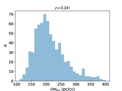
Figure 5: Distribution of $\mathrm{DM}_{\mathrm{IGM}}$ for $z_{\mathrm{frb}}=0.241$ sightlines in the Millennium simulation box, selected to intersect two $M_{\mathrm{halo}}>10^{14}\,M_{\odot}$ halos. The direct influence of groups and halos have been removed according to the selection function of Figure 4. We assume $f_{igm}=0.85$ for this calculation.

On the other hand, the FRB20190520B sightline intersects two separate galaxy clusters, which means that it must be crossing through overdense regions of the Universe even if we have already removed the direct influence of the clusters themselves within $\sim 1-2\,\mathrm{Mpc}$. For the $\langle{\rm DM}_{\rm IGM}\rangle$ calculation, we therefore selected mock sightlines at $z_{\mathrm{frb}}=0.241\pm 0.001$ that intersect within $r_{200}$ of two clusters with $M_{\mathrm{halo}}>10^{14}\,M_{\odot}$. Compared with randomly-selected sightlines at this redshift selected to originate within galaxies with an observed magnitude of $r<20$ (see, e.g., Pol et al. 2019), we find 0.07% of the sightlines intersect two separate foreground cluster halos, i.e. $\sim$ 1 in 1400.

We integrate the selected sightlines through Millenium density fields that have already been clipped of ‘observed’ clusters, and compute $\mathrm{DM}_{\mathrm{IGM}}$ assuming $f_{igm}=0.85$, which is a typical fraction of cosmic baryons expected to reside in the diffuse IGM as found in cosmological hydrodynamical simulations (e.g., Jaroszynski, 2019; Batten et al., 2021; Takahashi et al., 2021; Zhu & Feng, 2021; Zhang et al., 2021). The resulting $\mathrm{DM}_{\mathrm{IGM}}$ distribution is shown in Figure 5, with a median $\langle{\rm DM}_{\rm IGM}\rangle(z=0.241)=204^{+62}_{-39}\,\rm pc\,cm^{-3}$, where errors are quoted at the 16th and 84th percentiles. In comparison, for random sightlines at the same redshift through the normal ‘unclipped’ density field we find $\langle{\rm DM}_{\rm IGM}\rangle=191^{+64}_{-39}\,\rm pc\,cm^{-3}$, while for random sightlines through the clipped density fields we get $\langle{\rm DM}_{\rm IGM}\rangle=179^{+51}_{-33}$. The effects of clipping the influence of group/cluster halos and selecting sightlines that go through two clusters thus appear to largely cancel each other out, although the median $\mathrm{DM}_{\mathrm{IGM}}$ for our double-cluster sightlines is indeed slightly higher than the usual mean.

4.3 The Host DM of FRB20190520B

With the estimates of the foreground contributions in hand, we now subtract these from the total dispersion measure of FRB20190520B in order to constrain the host contribution. Since we the distributions for $\mathrm{DM}_{\mathrm{IGM}}$ and $\mathrm{DM}_{\mathrm{halos}}$ are significantly non-Gaussian, instead of propagating errors, we take the direct route of calculating the distribution of $\mathrm{DM}_{\mathrm{host}}$ based on the Monte Carlo realizations we have calculated for $\mathrm{DM}_{\mathrm{IGM}}$ and $\mathrm{DM}_{\mathrm{halos}}$.

In other words, we compute multiple iterations of:

$$\mathrm{DM}_{\mathrm{host},i}=\mathrm{DM}_{\mathrm{FRB},i}-\mathrm{DM}_{\mathrm{MW},i}-\mathrm{DM}_{\mathrm{IGM},i}\\ -\mathrm{DM}_{\mathrm{halos},i},$$ (5)

where $\mathrm{DM}_{\mathrm{halos},i}$ and $\mathrm{DM}_{\mathrm{IGM},i}$ were drawn from the Monte Carlo realizations computed in Sections 4.1 and 4.2, respectively. For $\mathrm{DM}_{\mathrm{FRB},i}$ and $\mathrm{DM}_{\mathrm{MW},i}$, we draw Gaussian random deviates for each iteration based on the values reported by Niu et al. (2022): $\mathrm{DM}_{\mathrm{FRB}}=(1205\pm 4)\,\rm pc\,cm^{-3}$ and ${\rm DM}_{\rm MW}=(113\pm 17)\,\rm pc\,cm^{-3}$, where the uncertainties are adopted as the Gaussian standard deviations. We enforced the prior that $\mathrm{DM}_{\mathrm{host}}\geq 0\,\rm pc\,cm^{-3}$.

After computing Equation 5 over $N=2000$ iterations, we computed the median and 16th/84th percentiles of the resulting $\mathrm{DM}_{\mathrm{host},i}$ distribution. These quantities, as well as the individual DM components, are listed in Table 3 — note that since the medians are listed for each component, they do not necessarily obey Equation 3 precisely.

Table 3: FRB20190520B DM Components

Component	$r_{max}=r_{200}$	$r_{max}=2\,r_{200}$
$\mathrm{DM}_{\mathrm{FRB}}$	$1205^{+4}_{-4}$
${\rm DM}_{\rm MW}$	$113^{+13}_{-13}$
$\mathrm{DM}_{\mathrm{IGM}}$	$204^{+62}_{-39}$
$\mathrm{DM}_{\mathrm{halos}}$	$450^{+240}_{-130}$	$640^{+260}_{-150}$
$\mathrm{DM}_{\mathrm{host}}$	$430^{+140}_{-220}$	$280^{+140}_{-170}$

We separately calculated the $\mathrm{DM}_{\mathrm{host}}$ for the two different assumptions of $r_{max}$ for the foreground halo contributions. Assuming $r_{max}=r_{200}$ (see Section 4.1), we find $\mathrm{DM}_{\mathrm{host}}=430^{+140}_{-220}\,\rm pc\,cm^{-3}$; on the other hand, for the $r_{max}=2\,r_{200}$ model, the resulting host contribution is $\mathrm{DM}_{\mathrm{host}}=280^{+140}_{-170}\,\rm pc\,cm^{-3}$ (both in the observed frame; the corresponding restframe values are $\mathrm{DM}_{\mathrm{host}}=540^{+170}_{-270}\,\rm pc\,cm^{-3}$ and $\mathrm{DM}_{\mathrm{host}}=350^{+180}_{-210}\,\rm pc\,cm^{-3}$, respectively). These estimates are much lower than the value of $\mathrm{DM}_{\mathrm{host}}=903^{+72}_{-111}\,\rm pc\,cm^{-3}$ originally reported by Niu et al. (2022). The 68th percentile errors we derive are significantly larger than the Niu et al. (2022) estimate, since they are driven by the uncertainties in the foreground cluster masses. Adopting the upper 68th percentile errors of our $\mathrm{DM}_{\mathrm{host}}$ values as a $\sigma$, the original estimate for $\mathrm{DM}_{\mathrm{host}}$ is $3.4\sigma$ and $4.3\sigma$ away from our $r_{max}=r_{200}$ and $r_{max}=2\,r_{200}$ model estimates, respectively.

5 Discussion

The $\mathrm{DM}_{\mathrm{host}}$ of FRBs arise from all the free electron contributions in the host galaxy and the immediate vicinity of the FRB, starting from the so-far mysterious source engine, ionized interstellar medium (ISM) gas, and then circumgalactic medium (CGM) of the host galaxy. For localized FRBs with a clearly identified host galaxy, it is in principle straightforward to calculate the halo mass and estimate the halo CGM contribution $\mathrm{DM}^{\mathrm{cgm}}_{\mathrm{host}}$ the same way we did for the foreground halos, so we can write

$$\mathrm{DM}_{\mathrm{host}}=\mathrm{DM}^{\mathrm{cgm}}_{\mathrm{host}}+\mathrm{DM}^{\mathrm{in}}_{\mathrm{host}},$$ (6)

where we define $\mathrm{DM}^{\mathrm{in}}_{\mathrm{host}}$ as the ‘inner’ DM components arising from the source engine and galaxy stellar/ISM component.

5.1 Host Halo Contribution

Given the association of FRB20190520B with the $z=0.241$ host galaxy HG20190520B by Niu et al. (2022), we can start by estimating the contribution from the CGM of the host halo. For the reported stellar mass of $M_{\star}\approx 6\times 10^{8}\,M_{\odot}$ (Niu et al., 2022), we use the dwarf galaxy stellar mass-halo mass relationship of Read et al. (2017) to estimate a halo mass of $M_{\mathrm{halo}}=9\times 10^{10}\,M_{\odot}$. Allowing for the fact that the FRB originates 5kpc (Niu et al. 2022) from the galaxy center, and adopting the models described in Section 4.1, we estimate restframe CGM contributions of $\mathrm{DM}^{\mathrm{cgm}}_{\mathrm{host}}=18\,\rm pc\,cm^{-3}$ and $\mathrm{DM}^{\mathrm{cgm}}_{\mathrm{host}}=12\,\rm pc\,cm^{-3}$ assuming the $r_{max}=r_{200}$ and $r_{max}=2\,r_{200}$ models, respectively. In other words, the CGM of HG20190520B yields but a small contribution to the $\mathrm{DM}_{\mathrm{host}}$ of FRB20190520B. This allows us to estimate restframe values of the inner host contribution to be $\mathrm{DM}^{\mathrm{in}}_{\mathrm{host}}\approx 520^{+170}_{-270}$ and $\mathrm{DM}^{\mathrm{in}}_{\mathrm{host}}\approx 330^{+180}_{-210}$, where we have neglected the error on $\mathrm{DM}^{\mathrm{cgm}}_{\mathrm{host}}$ due to the small central value.

5.2 Emission measures and scattering

In their analysis of FRB20190520B, Niu et al. (2022) and Ocker et al. (2022) had evaluated the emission measure (EM) from the observed optical H$\alpha$ lines in HG20190520B, which can be converted into an equivalent DM (Tendulkar et al., 2017). This was found to yield an observed frame value in the range $\mathrm{DM}_{\mathrm{host}}\approx 230-650\,\rm pc\,cm^{-3}$, which was in tension with the original estimate of $\mathrm{DM}_{\mathrm{host}}=903\,\rm pc\,cm^{-3}$. In comparison, our new estimate for the inner host contribution spans a 68 percentile confidence region of approximately $\mathrm{DM}_{\mathrm{host}}\sim 110-690\,\rm pc\,cm^{-3}$ (after combining results from both models in Section 4.1). The EM estimation is thus now in agreement with $\mathrm{DM}_{\mathrm{host}}$ without having to invoke unusually high gas temperatures ($T\gg 10^{4}\,K$) in the H$\alpha$ emitting medium as suggested by Ocker et al. (2022). Given the broad agreement between the EM and DM estimates, the H$\alpha$ emitting gas — presumably in the galaxy disk — also now appears to make up the bulk of the ionized medium responsible for the dispersion seen in HG20190520B.

Across a large number of repeating signals, FRB20190520B has also been measured by Ocker et al. (2022) to have a mean scattering time delay of $\tau=10.9\pm 1.5\,\mathrm{ms}$ (measured at 1.41 GHz) that can be attributed to the host. This DM of the scattering screen can be estimated from the scattering timescale using the expression from Cordes et al. (2022):

$$\tau(\mathrm{DM},\nu,z)\approx 48.03\,\mu s\;\times\;\frac{A_{\tau}\widetilde{F}G\,\mathrm{DM}^{2}}{(1+z_{\mathrm{frb}})^{3}\,\nu^{4}},$$ (7)

where $\nu$ is the measured frequency in GHz. The $A_{\tau}$ is a dimensionless quantity relating the mean scattering delay to the $1/e$ time, which we assume to be $A_{\tau}\approx 1$ following Ocker et al. (2022). The combined factor $\widetilde{F}G$ describes the combined amplification from turbulent density fluctuations and geometry of the scattering screen, respectively, which Ocker et al. (2022) estimate to be $\widetilde{F}G=1.5^{+0.8}_{-0.3}\,(\mathrm{pc^{2}\;km})^{-1/3}$ using the old value of $\mathrm{DM}_{\mathrm{host}}=903\,\rm pc\,cm^{-3}$.

With our updated restframe $\mathrm{DM}^{\mathrm{in}}_{\mathrm{host}}$ values for FRB20190520B (Section 5.1), we recalculate $\widetilde{F}G\propto 1/\mathrm{DM}^{2}$ to find $\widetilde{F}G\approx 4.5-11\,(\mathrm{pc^{2}\;km})^{-1/3}$, with the range allowing for our model uncertainty in subtracting off the foreground galaxy clusters. This constrasts with the value originally estimated by Ocker et al. (2022), which is close to unity. This larger value implies that either $\widetilde{F}>1$ or $G>1$, or both. If $\widetilde{F}>1$ it would imply that the scattering screen is highly turbulent. Meanwhile, $G\approx 1$ is expected if the turbulent scattering screen is close to the source, but could be greater than unity if the screen is somewhere along the intervening path yet still farther away from the Milky Way, e.g. if they were associated with the foreground clusters. However, Connor et al. (2023) recently studied two FRBs that were localized to host galaxies embedded within galaxy clusters, and did not see significant scattering in those FRB signals. We therefore consider it unlikely that foreground clusters are the source of the scattering; it is more likely that the large $\widetilde{F}G$ value is due to a highly turbulent scattering screen associated with the host and perhaps even close to the FRB engine itself. This conclusion is corroborated by the recent Ocker et al. (2023) paper which reports significant scattering variations in the repeated FRB20190520B signals, as well as the sign-changes observed in their Faraday rotation (Anna-Thomas et al., 2023).

5.3 FRB20190520B in Context

When FRB20190520B was discovered, its $\mathrm{DM}_{\mathrm{host}}$ estimate and those of nearly all other localized FRBs were done through guesstimated $\mathrm{DM}_{\mathrm{host}}$ values after subtracting the mean $\langle{\rm DM}_{\rm IGM}\rangle(z)$. At this time of writing, approximately a half-dozen localized FRBs now have credible foreground analyses that enable more confidence in their estimated $\mathrm{DM}_{\mathrm{host}}$.

Arguably the first reliable estimate was done by Simha et al. (2020), who analyzed the foreground of FRB20190608 based on Sloan Digital Sky Survey (SDSS) and Keck data using an analogous technique to ours. They estimate $\mathrm{DM}_{\mathrm{host}}\approx 80-200\,\rm pc\,cm^{-3}$ (observed frame), which is in fact consistent with an independent analysis of the host galaxy (Chittidi et al., 2021).

More recently, Simha et al. (2023) analyzed 4 FRB sightlines known to exhibit DMs significantly higher than the cosmic mean, using FLIMFLAM spectroscopic data of the foreground fields.

FRB20210117A was, like FRB20190520B, suspected to be a high $\mathrm{DM}_{\mathrm{host}}$ source given its clear excess $\mathrm{DM}_{\mathrm{FRB}}=731\,\rm pc\,cm^{-3}$ and its localized redshift of $z_{\mathrm{frb}}=0.2145$. However, unlike FRB20190520B no significant excess was found from $\mathrm{DM}_{\mathrm{halos}}$ based on the foreground data, and so it is confirmed to be a high-$\mathrm{DM}_{\mathrm{host}}$ source, with $\mathrm{DM}_{\mathrm{host}}\approx 665\,\rm pc\,cm^{-3}$ in the restframe. This is in fact higher than the revised restframe values of $\mathrm{DM}_{\mathrm{host}}\sim 350-540\,\rm pc\,cm^{-3}$ we now find for FRB20190520B, which now makes FRB20210117A in principle the FRB with the highest known $\mathrm{DM}_{\mathrm{host}}$, although the uncertainties are large enough for either to be the true record holder. FRB20200906A was also shown to not have significant foreground contributions despite a high $\mathrm{DM}_{\mathrm{FRB}}$, yielding an estimate of $\mathrm{DM}_{\mathrm{host}}\approx 420\,\rm pc\,cm^{-3}$. FRB20190714A and FRB20200430A are shown to have significant foreground contributions, thus they do not have large $\mathrm{DM}_{\mathrm{host}}$. We note that this sub-sample is explicitly biased towards excess-DM sources, and thus it possible that the $\mathrm{DM}_{\mathrm{host}}$ from this sample might be biased high as well even though some of the FRBs are shown to be from overdense foregrounds.

James et al. (2022) and subsequently Baptista et al. (2023) have performed population modeling of a sample of $\approx 70$ FRBs including 21 with redshifts from host associations. Their forward model includes two parameters to desribe a log-normal distribution for $\mathrm{DM}_{\mathrm{host}}$. Taking their preferred values of $\sigma=0.5$ and $\mu=2.43$, we find that 40% of FRB hosts are expected to have $\mathrm{DM}_{\mathrm{host}}>500\,\rm pc\,cm^{-3}$. We conclude, therefore, that our inferred value for FRB20190520B is consistent with the full population.

6 Conclusion

In this paper, we used wide-field spectroscopic data from the FLIMFLAM survey targeting the field of FRB20190520B to study the possible foreground contributions to the overall observed DM, which is anomalously high ($\mathrm{DM}_{\mathrm{FRB}}$= 1205 $\rm pc\,cm^{-3}$) given its confirmed redshift. Our data shows that the FRB20190520B sightline directly intersects two foreground galaxy clusters, at $z=0.1867$ and $z=0.2170$, within their virial radius, in a rare occurrence estimated to happen to only $\sim$1 in 1400 sightlines at this FRB pathlength. These two foreground clusters yield a combined contribution of $\mathrm{DM}_{\mathrm{halos}}\sim 450-640\,\rm pc\,cm^{-3}$, which allows us to revise the host contribution downwards to $\mathrm{DM}_{\mathrm{host}}\sim 280-430\,\rm pc\,cm^{-3}$ after also taking account the Milky Way and diffuse IGM contributions (see Table 3 for detailed values). This means that FRB20190520B is no longer the FRB with the largest host DM contribution, with FRB20210117A now being the source with the largest known $\mathrm{DM}_{\mathrm{host}}$, but they are similar to within the uncertainties. The new value for $\mathrm{DM}_{\mathrm{host}}$ is now in agreement with H$\alpha$ emission estimates of $\mathrm{DM}_{\mathrm{host}}$, and also allowed us to make a revised estimate of the combined factor describing geometric effects and turbulent density fluctuations based on the scattering time scale: $\widetilde{F}G\approx 4.5-11\,(\mathrm{pc^{2}\;km})^{-1/3}$. We interpret this as due to high turbulence in the scattering screen associated with the host, since we consider it unlikely that the foreground halos are the source of the scattering.

This result outlines the importance of obtaining sufficiently wide-field foreground spectroscopy in disentangling the various DM contributions in FRBs, both for their usage as cosmological probes as well as for understanding their host progenitors. The original Keck/LRIS optical spectroscopy from Niu et al. (2022) were single-slit observations, but even if they had utilized multi-object slitmasks to target some of the foreground galaxies, they would have been limited to within 2-3$\arcmin$ of the FRB position by the limited field of view of LRIS (see the interactive version of Figure 2). LRIS observations might have captured 2-3 of the $z_{\mathrm{grp}}=0.1867$ group members, but the rest lie 4-5$\arcmin$ away from the FRB. The member galaxies of the $z_{\mathrm{grp}}=0.2170$ group, on the other hand, lie mostly $\sim 5-6\arcmin$ away from FRB20190520B and would likely have been missed even with multi-object spectroscopy with LRIS or equivalent narrow-field spectrographs on other telescopes.

Our present result on FRB20190520B is a vivid illustration of the power of foreground data in enhancing the use of FRBs. In Lee et al. (2022), we had estimated that wide-field foreground spectroscopy enhances the power of localized FRBs as cosmological probes by a factor of $\sim 30$ in terms of the number of FRBs required to achieve comparable constraints — whereas in comparison with unlocalized FRBs, this is an enhancement is up to $\sim 10^{2}-10^{3}$ (Shirasaki et al., 2022; Wu & McQuinn, 2023).

In an upcoming paper (Khrykin et al, in prep), we will present the first cosmic baryon analysis from a preliminary sample of FLIMFLAM fields, that will give the first constraints on the partition of cosmic baryons between the IGM and CGM.

References

- Anna-Thomas et al. (2023) Anna-Thomas, R., Connor, L., Dai, S., et al. 2023, Science, 380, 599, doi: 10.1126/science.abo6526
- Astropy Collaboration et al. (2022) Astropy Collaboration, Price-Whelan, A. M., Lim, P. L., et al. 2022, ApJ, 935, 167, doi: 10.3847/1538-4357/ac7c74
- Ata et al. (2015) Ata, M., Kitaura, F.-S., & Müller, V. 2015, MNRAS, 446, 4250, doi: 10.1093/mnras/stu2347
- Ayromlou et al. (2022) Ayromlou, M., Nelson, D., & Pillepich, A. 2022, arXiv e-prints, arXiv:2211.07659. https://arxiv.org/abs/2211.07659
- Baptista et al. (2023) Baptista, J., Prochaska, J. X., Mannings, A. G., et al. 2023, arXiv e-prints, arXiv:2305.07022, doi: 10.48550/arXiv.2305.07022
- Batten et al. (2021) Batten, A. J., Duffy, A. R., Wijers, N. A., et al. 2021, MNRAS, 505, 5356, doi: 10.1093/mnras/stab1528
- Bertin & Arnouts (1996) Bertin, E., & Arnouts, S. 1996, A&AS, 117, 393, doi: 10.1051/aas:1996164
- Boquien et al. (2019) Boquien, M., Burgarella, D., Roehlly, Y., et al. 2019, A&A, 622, A103, doi: 10.1051/0004-6361/201834156
- Childress et al. (2017) Childress, M. J., Lidman, C., Davis, T. M., et al. 2017, MNRAS, 472, 273, doi: 10.1093/mnras/stx1872
- Chittidi et al. (2021) Chittidi, J. S., Simha, S., Mannings, A., et al. 2021, ApJ, 922, 173, doi: 10.3847/1538-4357/ac2818
- Chiu et al. (2018) Chiu, I., Mohr, J. J., McDonald, M., et al. 2018, MNRAS, 478, 3072, doi: 10.1093/mnras/sty1284
- Connor et al. (2023) Connor, L., Ravi, V., Catha, M., et al. 2023, ApJ, 949, L26, doi: 10.3847/2041-8213/acd3ea
- Cook et al. (2023) Cook, A. M., Bhardwaj, M., Gaensler, B. M., et al. 2023, ApJ, 946, 58, doi: 10.3847/1538-4357/acbbd0
- Cordes & Lazio (2002) Cordes, J. M., & Lazio, T. J. W. 2002, arXiv e-prints, astro, doi: 10.48550/arXiv.astro-ph/0207156
- Cordes et al. (2022) Cordes, J. M., Ocker, S. K., & Chatterjee, S. 2022, ApJ, 931, 88, doi: 10.3847/1538-4357/ac6873
- Gonzalez et al. (2013) Gonzalez, A. H., Sivanandam, S., Zabludoff, A. I., & Zaritsky, D. 2013, ApJ, 778, 14, doi: 10.1088/0004-637X/778/1/14
- Guo et al. (2011) Guo, Q., White, S., Boylan-Kolchin, M., et al. 2011, MNRAS, 413, 101, doi: 10.1111/j.1365-2966.2010.18114.x
- Harris et al. (2020) Harris, C. R., Millman, K. J., van der Walt, S. J., et al. 2020, Nature, 585, 357, doi: 10.1038/s41586-020-2649-2
- Henriques et al. (2015) Henriques, B. M. B., White, S. D. M., Thomas, P. A., et al. 2015, MNRAS, 451, 2663, doi: 10.1093/mnras/stv705
- Hinton et al. (2016) Hinton, S. R., Davis, T. M., Lidman, C., Glazebrook, K., & Lewis, G. F. 2016, Astronomy and Computing, 15, 61, doi: 10.1016/j.ascom.2016.03.001
- Horowitz et al. (2019) Horowitz, B., Lee, K.-G., White, M., Krolewski, A., & Ata, M. 2019, ApJ, 887, 61, doi: 10.3847/1538-4357/ab4d4c
- Hunter (2007) Hunter, J. D. 2007, Computing in Science and Engineering, 9, 90, doi: 10.1109/MCSE.2007.55
- Inoue (2004) Inoue, S. 2004, MNRAS, 348, 999, doi: 10.1111/j.1365-2966.2004.07359.x
- Ioka (2003) Ioka, K. 2003, ApJ, 598, L79, doi: 10.1086/380598
- James et al. (2022) James, C. W., Ghosh, E. M., Prochaska, J. X., et al. 2022, MNRAS, 516, 4862, doi: 10.1093/mnras/stac2524
- Jaroszynski (2019) Jaroszynski, M. 2019, MNRAS, 484, 1637, doi: 10.1093/mnras/sty3529
- Kitaura et al. (2021) Kitaura, F.-S., Ata, M., Rodríguez-Torres, S. A., et al. 2021, MNRAS, 502, 3456, doi: 10.1093/mnras/staa3774
- Law et al. (2018) Law, C. J., Bower, G. C., Burke-Spolaor, S., et al. 2018, ApJS, 236, 8, doi: 10.3847/1538-4365/aab77b
- Lee et al. (2022) Lee, K.-G., Ata, M., Khrykin, I. S., et al. 2022, ApJ, 928, 9, doi: 10.3847/1538-4357/ac4f62
- Li et al. (2018) Li, D., Wang, P., Qian, L., et al. 2018, IEEE Microwave Magazine, 19, 112, doi: 10.1109/MMM.2018.2802178
- Macquart et al. (2020) Macquart, J. P., Prochaska, J. X., McQuinn, M., et al. 2020, Nature, 581, 391, doi: 10.1038/s41586-020-2300-2
- Maller & Bullock (2004) Maller, A. H., & Bullock, J. S. 2004, MNRAS, 355, 694, doi: 10.1111/j.1365-2966.2004.08349.x
- Mathews & Prochaska (2017) Mathews, W. G., & Prochaska, J. X. 2017, ApJ, 846, L24, doi: 10.3847/2041-8213/aa8861
- Miszalski et al. (2006) Miszalski, B., Shortridge, K., Saunders, W., Parker, Q. A., & Croom, S. M. 2006, MNRAS, 371, 1537, doi: 10.1111/j.1365-2966.2006.10777.x
- Moster et al. (2013) Moster, B. P., Naab, T., & White, S. D. M. 2013, MNRAS, 428, 3121, doi: 10.1093/mnras/sts261
- Nan et al. (2011) Nan, R., Li, D., Jin, C., et al. 2011, International Journal of Modern Physics D, 20, 989, doi: 10.1142/S0218271811019335
- Navarro et al. (1997) Navarro, J. F., Frenk, C. S., & White, S. D. M. 1997, ApJ, 490, 493, doi: 10.1086/304888
- Niu et al. (2022) Niu, C. H., Aggarwal, K., Li, D., et al. 2022, Nature, 606, 873, doi: 10.1038/s41586-022-04755-5
- Ocker et al. (2023) Ocker, S. K., Cordes, J. M., Chatterjee, S., et al. 2023, MNRAS, 519, 821, doi: 10.1093/mnras/stac3547
- Ocker et al. (2022) —. 2022, ApJ, 931, 87, doi: 10.3847/1538-4357/ac6504
- Pol et al. (2019) Pol, N., Lam, M. T., McLaughlin, M. A., Lazio, T. J. W., & Cordes, J. M. 2019, ApJ, 886, 135, doi: 10.3847/1538-4357/ab4c2f
- Prochaska & Zheng (2019) Prochaska, J. X., & Zheng, Y. 2019, MNRAS, 485, 648, doi: 10.1093/mnras/stz261
- Ravi et al. (2023) Ravi, V., Catha, M., Chen, G., et al. 2023, arXiv e-prints, arXiv:2301.01000, doi: 10.48550/arXiv.2301.01000
- Read et al. (2017) Read, J. I., Iorio, G., Agertz, O., & Fraternali, F. 2017, MNRAS, 467, 2019, doi: 10.1093/mnras/stx147
- Schlafly & Finkbeiner (2011) Schlafly, E. F., & Finkbeiner, D. P. 2011, ApJ, 737, 103, doi: 10.1088/0004-637X/737/2/103
- Shirasaki et al. (2022) Shirasaki, M., Takahashi, R., Osato, K., & Ioka, K. 2022, MNRAS, 512, 1730, doi: 10.1093/mnras/stac490
- Simha et al. (2020) Simha, S., Burchett, J. N., Prochaska, J. X., et al. 2020, ApJ, 901, 134, doi: 10.3847/1538-4357/abafc3
- Simha et al. (2021) Simha, S., Tejos, N., Prochaska, J. X., et al. 2021, arXiv e-prints, arXiv:2108.09881. https://arxiv.org/abs/2108.09881
- Simha et al. (2023) Simha, S., Lee, K.-G., Prochaska, J. X., et al. 2023, arXiv e-prints, arXiv:2303.07387, doi: 10.48550/arXiv.2303.07387
- Sorini et al. (2022) Sorini, D., Davé, R., Cui, W., & Appleby, S. 2022, MNRAS, 516, 883, doi: 10.1093/mnras/stac2214
- Springel (2005) Springel, V. 2005, MNRAS, 364, 1105, doi: 10.1111/j.1365-2966.2005.09655.x
- Tago et al. (2008) Tago, E., Einasto, J., Saar, E., et al. 2008, A&A, 479, 927, doi: 10.1051/0004-6361:20078036
- Takahashi et al. (2021) Takahashi, R., Ioka, K., Mori, A., & Funahashi, K. 2021, MNRAS, 502, 2615, doi: 10.1093/mnras/stab170
- Tempel et al. (2012) Tempel, E., Tago, E., & Liivamägi, L. J. 2012, A&A, 540, A106, doi: 10.1051/0004-6361/201118687
- Tempel et al. (2014) Tempel, E., Tamm, A., Gramann, M., et al. 2014, A&A, 566, A1, doi: 10.1051/0004-6361/201423585
- Tendulkar et al. (2017) Tendulkar, S. P., Bassa, C. G., Cordes, J. M., et al. 2017, ApJ, 834, L7, doi: 10.3847/2041-8213/834/2/L7
- Virtanen et al. (2020) Virtanen, P., Gommers, R., Oliphant, T. E., et al. 2020, Nature Methods, 17, 261, doi: 10.1038/s41592-019-0686-2
- Wu & McQuinn (2023) Wu, X., & McQuinn, M. 2023, ApJ, 945, 87, doi: 10.3847/1538-4357/acbc7d
- Yao et al. (2017) Yao, J. M., Manchester, R. N., & Wang, N. 2017, ApJ, 835, 29, doi: 10.3847/1538-4357/835/1/29
- Yuan et al. (2015) Yuan, F., Lidman, C., Davis, T. M., et al. 2015, MNRAS, 452, 3047, doi: 10.1093/mnras/stv1507
- Zhang et al. (2021) Zhang, Z. J., Yan, K., Li, C. M., Zhang, G. Q., & Wang, F. Y. 2021, ApJ, 906, 49, doi: 10.3847/1538-4357/abceb9
- Zhu & Feng (2021) Zhu, W., & Feng, L.-L. 2021, ApJ, 906, 95, doi: 10.3847/1538-4357/abcb90