Rate Forecaster based Energy Aware Band Assignment in Multiband Networks

Abstract

The high frequency communication bands (mmWave and sub-THz) promise tremendous data rates, however, they also have very high power consumption which is particularly significant for battery-power-limited user-equipment (UE). In this context, we design an energy aware band assignment system which reduces the power consumption while also achieving a target sum rate of $M$ in $T$ time-slots. We do this by using 1) Rate forecaster(s); 2) Channel forecaster(s) which forecasts $T$ direct multistep ahead using a stacked (long short term memory) LSTM architecture. We propose an iterative rate updating algorithm which updates the target rate based on current rate and future predicted rates in a frame. The proposed approach is validated on the publicly available ‘DeepMIMO’ dataset. Research findings shows that the rate forecaster based approach performs better than the channel forecaster. Furthermore, LSTM based predictions outperforms well celebrated Transformer predictions in terms of NRMSE and NMAE. Research findings reveals that the power consumption with this approach is $\sim 300$ mW lower compared to a greedy band assignment at a 1.5Gb/s target rate.

I Introduction

The 3GPP has considered significant available bandwidth at millimeter (mmWave) frequencies in its fifth generation new radio (5G-NR) standard, and potentially also considering Sub-THz bands (>100 GHz) which would help achieve beyond5G/6G objectives [1]. Although the mmWave and THz bands provide significant bandwidth and promise tremendously high data rates (ranging from multi-gigabit-per-second up to terabit-per-second), propagation at these bands is limited by severe path loss, and is susceptible to blockages. These factors limit the quality of service and user experience [2].

Due to the complementary characteristics of wireless signal propagation at Sub-6 GHz and mmWave bands, 3GPP standards have also evolved to support multiband networks [3], leading to the band assignment problem. There are several works in the literature that have investigated the band assignment problem in multiband heterogeneous systems, e.g. [4, 5, 6]. Recently, few works have applied machine learning (ML) techniques in context of band assignment. For instance, a supervised ML based approach for band switching in dual band systems was studied in [7]. A deep neural network (DNN) based band switching in dual band systems was proposed in [8], while deep reinforcement learning (DRL) for band switching in unmanned aerial vehicle (UAV) was analyzed in [9].

Most of the aforementioned works considered the criteria of achieving the maximum rate in band assignment. Although the higher frequency bands promise a very high data rate, the power consumption is significantly different in different bands, e.g., more than an order of magnitude higher in THz than in mmWave bands [10]. Since the battery power in user equipment (UE) is limited, it is desirable for future green networks that the band assignment policies not only consider the rate criteria but also the power consumed. A heuristic approach for dual bands (Sub-6 GHz and mmWave) was considered in our previous work [11] wherein if the power consumed in a recent time window exceeds a certain threshold, a band switch would be initiated to a lower-power-consuming band, without consideration of the rate to be achieved.

With the possibility of forecasting rate in future time slots, enabled by advances in ML, an energy-aware base station (BS) may choose to not utilize a high-rate, high energy consuming band (or it may choose to not transmit at all) at a given time-slot if it predicts that the rate will be significantly higher in a later time slot. Such an approach can lead to improved energy usage in systems where the highest possible rate is not always necessary. On the other hand, such an approach might lead to long delays if the BS waits for favorable channel conditions before transmitting in a high frequency, high-energy-cost band. Therefore, to make such a system practical, some form of time limitation is necessary. To the best of the authors’ knowledge, such an approach which considers to minimize the power consumption and still meet the target rate in a given time constraint using rate forecast in future time slots, although promising, has not been reported in the literature.

In this context, we consider energy aware operation of downlink multiband networks. Given the battery power limitation of UE, we only consider the power consumption of the UE and not the BS. In each slot of a frame, the BS chooses which band to transmit in to meet a target sum rate in the frame (proportional to the number of bits transmitted in the frame), with the lowest average UE power consumption in that frame. The choice of which band to utilize in this work is enabled by the use of multiple rate/channel forecasters which predict rates in future time slots based on learned past history of a moving UE, and other UEs with similar (but not the same) trajectory. The key contributions can be summarized as:

• A novel framework for energy aware band assignment in multiband networks which minimizes power consumption while attempting to achieve a target average rate per frame.

• An iterative procedure for band assignment which utilizes rate/channel predictions for varying number of future slots is introduced. This approach can be applied to any rate/channel forecasting algorithm.

• We design rate and channel forecasters which forecast direct multistep ahead for future time slots. We propose a stacked long short term memory (LSTM) as a forecaster(s). We tailor the publicly available ray-tracing based ‘DeepMIMO’ dataset [12] for motion and apply this approach to it. The proposed approach outperforms several other approaches considered. Furthermore, simulation results reveals the LSTM forecaster also outperforms the Transformer model, which has received a lot of attention recently.

II System model and Problem Formulation

II-A Network and System Model

In this work, we consider a multiband network in which both the BS and mobile UEs can operate in the Sub-6 GHz, mmWave or THz bands. We assume that the BS is equipped with multiple antennas (3D array). As per the UE design in [10] and references therein, for UEs, we assume a single antenna at Sub6 (3.5 GHz), an array with $N_{Rx}=8$ antennas at mmWave (28 GHz), and an array with $N_{Rx}=64$ antenna elements at THz band (140 GHz). For ease of notation, we use $i\in(\text{NoTx, Sub-6, mmWave, THz})$ to denote no-transmission case and the three bands, and at any time slot, the BS can only utilize one of the bands or not transmit at all. In slot $t$, the baseband equivalent of the received signal at the UE, transmitted by the BS in band $i$ can be written as [8]:

$$\small y_{i}[t]=\sqrt{\text{P}_{T_{X_{i}}}}\hskip 2.84526pt\textbf{\text{h}}^{*}_{i}[t]\hskip 2.84526pt\textbf{\text{f}}_{i}[t]\hskip 2.84526ptx_{i}[t]+w_{i}[t],$$ (1)

where, $\text{P}_{T_{X_{i}}}$ is the transmitted power by BS in $i^{\text{th}}$ band, $\textbf{\text{h}}_{i}[t]$ $\in\mathbb{C}^{N_{Tx}}$ is the channel vector, $\textbf{\text{f}}_{i}[t]$ is the beam forming vector at $t$ time slot, $x_{i}[t]$ is the transmitted signal, and $w_{i}[t]$ is the additive white Gaussian noise with zero mean and variance $\sigma^{2}_{i}$ in the $i$-th band. The evolution of $\mathbf{h}_{i}[t]$ over time is based on the motion of the UE and is described in more detail in Section III-B.

We assume that the BS performs maximal ratio transmission where $\textbf{f}_{i}[t]=\frac{1}{|\textbf{h}_{i}[t]|}\textbf{h}_{i}[t]$. Accordingly, the received SNR on the $i^{\text{th}}$ frequency band with $N_{Rx}$ receive antennas is

$$\small\gamma_{i}[t]=\frac{\text{P}_{T_{X_{i}}}}{\sigma_{i}^{2}}N_{Rx}\hskip 2.84526pt|\text{{h}}_{i}[t]|^{2},$$ (2)

Note that we have made the assumption that the SNR with multiple receive antennas is equal to the SNR with one receive antenna multiplied by the number of antennas. This assumption enables us to easily use datasets generated for UEs with isotropic antennas. The achievable rate in slot $t$ can be written as:

$$\small R_{i}[t]=B_{i}\hskip 2.84526pt\text{log}_{2}\{1+\gamma_{i}[t]\},$$ (3)

where $B_{i}$ is the bandwidth of the $i^{\text{th}}$ frequency band, with $B_{\text{NoTx}}=0$. We assume that the BS is equipped with a forecaster and learns from past history of other UEs to make energy aware band assignments.

II-B Power Consumption in Sub-6, mmWave, and THz band

Since the UEs can operate in Sub-6, mmWave, or the THz bands, the power consumed by the RF chains will be significantly different. The estimates of power consumed by the major components in the RF chains is summarized in Table I, and can be expressed as:

Table I: Power consumption of RF components (in mW)

Component	Sub-6 (3.5GHz)	mmWave (28GHz)	THz band (140GHz)
Bandpass filter (BPF)	5	5	5
Low Noise Amplifier (LNA)	10	11.13	50.89
Local Oscillator (LO)	5	5	5
Phase Shifter (PS)	-	1.5	1.5
Combiner	-	19.5	19.5
Mixer	15	16.8	49
Low Pass Filter (LPF)	10	14	11.36
Baseband Amplifier (BBA)	5	5	5
Analog to Digital Converter (ADC)	7.8	8.2	32.7

$$\small\begin{split}\text{P}_{i}&=N_{i-Rx}(\text{P}_{i-\texttt{BPF}}+\text{P}_{i-\texttt{LNA}}+\text{P}_{i-\texttt{PS}})+\text{P}_{i-\texttt{Combiner}}+\text{P}_{i-\texttt{LO}}+\\ &\hskip 71.13188pt2(\text{P}_{i-\texttt{Mixer}}+\text{P}_{i-\texttt{LPF}}+\text{P}_{i-\texttt{BBA}}+\text{P}_{i-\texttt{ADC}}).\end{split}$$ (4)

The factor-2 in (4) is due to the inphase and quadrature phase components. On substituting the values of each component in (4) based on [10, 13, 14, 15] and references therein, the approximate power consumed by the RF chain of the UE in Sub-6 GHz, mmWave and THz bands are $\text{P}_{\text{Sub-6}}=85.60$ mW, $\text{P}_{\text{mmWave}}=254.90$ mW and $\text{P}_{\text{THz}}=3893.58$ mW, respectively. Note that the power consumption is more than an order of magnitude higher in the THz than in the mmWave and Sub-6 GHz bands. Thus, our aim is to design an energy aware band assignment approach which minimizes the power consumption subject to a target sum/average rate per frame, which is mathematically formulated in the next subsection.

II-C Problem Formulation

To minimize the energy usage, one option is to never transmit and thus power consumption would be minimal, which is unrealistic. Thus, we introduce a target rate that the BS will try to achieve at the UE. Further, in trying to achieve a sum target rate in a manner that is energy efficient, the BS may wait for a long time for favorable channel conditions before transmitting at all, or before transmitting in a high frequency, high energy-cost band. Such an approach could lead to extremely long delays. Thus, we introduce a delay constraint $T$. We assume a time slotted communication, with a frame comprising of $T$ time slots. The aim of the BS is to achieve a target sum-rate $M$ in every frame, while utilizing the lowest average power during that frame at the UE. Further, we assume that the BS can choose which band to transmit in for each slot, or choose not to transmit at all in a given slot.

With the aid of eq. (3), for a given frame with $T$ slots and $i_{t}$ representing the band in the $t$-th slot during the frame, we wish to find $i_{t}$’s to

$$\text{min.}\hskip 5.69054pt\text{P}_{\text{consumed}}=\sum_{t=1}^{T}{\text{P}_{i_{t}}},$$

$${\rm s}.{\rm t}.\hskip 2.84526ptM \leq\sum_{t=1}^{T}\left(1-\nu\mathbbm{1}_{\{i_{t}\neq i_{t-1}\}}\right)B_{i_{t}}\hskip 2.84526pt\text{log}_{2}\left(1+\frac{\text{P}_{\text{Tx}_{i_{t}}}\hskip 2.84526pt|\text{{h}}_{i_{t}}[t]|^{2}}{\sigma_{i_{t}}^{2}}\right)$$ (5)

where $\text{P}_{T_{X_{i}}}$ is the BS transmit power in the $i^{th}$ band, $\nu\in[0,1)$ is a switching cost which models the overhead time required to switch bands, and $\mathbbm{1}$ is an indicator function. We are showing the equations just for a single frame, to simplify notation. Our objective is to minimize the average consumed power in each frame subject to the target average rate in that frame. In other words, we attempt to minimize $\sum_{t=1}^{T}P_{i_{t}}$ subject to (5). If (5) is not achievable, then we aim to maximize the RHS of (5).

Note that if channel coefficients/rates of future time slots were known, the optimal channel assignment can be done by exhaustive search. Since future channels cannot be known at a prior time slot, the BS predicts the rate/channel conditions in future time slots to make its decision on which band to use in the current time slot. In this work, the choice of which band to transmit in is enabled by the use of multiple rate forecasters which predict rates in future time slots based on learned past history, which is discussed in the next section. We would like to highlight that the rate in eq. (5) can be forecasted by: 1) Forecasting the $\text{log}_{2}\left(1+\gamma\right)$ term, which we refer to as rate forecaster, or 2) By forecasting the $|\text{{h}}_{i}[t]|^{2}$, which we refer to as channel forecaster.

III Proposed Scheme & Methodology

III-A Proposed scheme

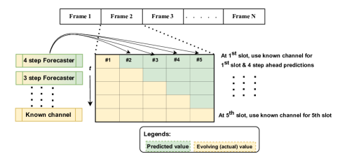
Figure 1: Framework of the proposed scheme.

The framework of the proposed scheme is as shown in Fig. 1 and complemented with algorithm-1 & 2. Assume that each frame is comprised of $T=5$ slots for illustration (any number $T>1$ could work). At each time, the BS can either not transmit or utilize one of the Sub6, mmWave, or THz bands. Thus, there are total four options i.e., Sub6/mmWave/THz/no transmit, of which one is to be selected in each time slot. For better understanding, a grid structure is shown wherein the rows are the time indices, and columns are the slots. We propose to use ‘$T$’ forecasters, each predicting ‘$T$’ direct multistep ahead i.e., 4 step forecaster predicts 4 direct step ahead continuous values. Thus, in the first slot, the 4 step forecaster would be used to predict the rate/channel values for all the future time slots in the frame, where we assume that the rate/channel in the current slot is known. The forecasted values are highlighted by the green boxes in the first row of the grid. Since rate/channel predictions for future slots become less reliable (particularly for THz), we reduce the channel predictions further into the future to account for this fact. We do so by multiplying rates/channels for the THz forecast by factors of 0.85, 0.8, 0.75, and 0.7 for the predictions 1 - 4 steps into the future respectively (algorithm-1, upto line 13). Next, the optimal band assignment is done for all the five slots, using an exhaustive search. This is shown in algorithm-2. For each frame, it iterates over all the possible combinations i.e., $4^{T}$ options of band assignments (plus the no-transmit option), to obtain the set of 5 band assignments which consumes the minimum energy, and is predicted to meet the target rate. The resulting band assignment for the first slot is selected as the band to use in this slot (in algorithm-1). The rate achieved in this slot is computed and subtracted from the sum-rate threshold (algorithm-1, line 17) to compute a new threshold for the next time slot. Next, at the $2^{nd}$ time slot, we use the exact channel in the second slot and 3 step ahead predictions and so on. At each time slot, the optimal band assignment procedure would be called with successively smaller number of slots to reflect the declining number of slots remaining in the current frame. The rate threshold would updated each slot by subtracting the rate already achieved in the previous time slot(s). This process will be repeated for all the slots. The proposed algorithm is described in algorithm-1, where for a given frame, $\hat{R}_{i}[\ell,t]$ is the predicted rate for the $\ell$-th slot of the $i$-th band, as predicted in the $t$-th slot. The rate forecasters predict $\hat{R}_{i}[\ell,t]$ directly and the channel predictors use (3) and (2) with predictions of $|\mathbf{h}_{i}[t]|^{2}$.

The proposed design serves as an energy aware band assignment schemes which is motivated by systems with a finite battery life, which takes advantage of the fact that rate/channel forecasts for slots longer in the future will be less accurate than forecasts for slots closer in the future.

Algorithm 1 Proposed algorithm

1:procedure Proposed Approach

2:     Import O1 scenario; select UEs, BS locations

3:     Run ray traces for the settings specified

4:     Specify $M$, Power consumed in each band

5:     Built and model $T$ separate forecasters.

6:     Each forecaster predicts $T$ continuous predictions

7:     Load the forecasted values

8:     for $m=1$ : all frames do

9:         for $t=1$ : $T$ do

10:              Obtain $R_{i}[t]$ for $i=1,2,3$

11:              Get $\hat{R}_{i}[t+1,t]\cdots\hat{R}_{i}[T,t]$, $i=1,2,3$

12:              $\hat{R}(i_{t},i_{t+1},\cdots i_{T})\leftarrow R_{i_{t}}[t]+\sum_{k=t+1}^{T}\hat{R}_{i_{k}}[k],$

13:               $\forall(i_{t},\cdots i_{T})\in\{\text{NoTx,Sub6,mmWave,THz}\}^{T-t+1}$

14:              Call Optimal Bandassignment with

15:                $\hat{R}(i_{t},i_{t+1},\cdots i_{T}),M,T-t+1$

16:              $b_{t}\leftarrow$ slot $t$ assignment by Opt. Bandassignment

17:              $M\leftarrow M-R_{b_{t}}[t]$          

18:         Compute power consumed in frame.

19:         Compute sum rate in frame.      

20:     Compute average power consumed per frame.

Algorithm 2 Optimal Band Assignment algorithm

1:procedure Optimal BandAssignment($\hat{R}(i_{t},\cdots i_{T}),M,T$)

2:     for $k=1:4^{T}$  do

3:         Loop over all the possible band combinations

4:         Compute corresponding sum rates ($R$)

5:         Save the band combinations where $R>$ $M$      

6:     if Indices where $R>M\neq\emptyset$  then

7:         Return band assignments where energy is min.

8:     else

9:         Return band assignments where rate is max.      

10:The above procedure yields the best band assignments for each frame that satisfies our objective in (5).

III-B Dataset Construction and Processing

The proposed algorithm was evaluated on the ‘DeepMIMO’ dataset [12]. In particular, we consider the ray-tracing outdoor scenario-1 ‘O1_3p5’ for Sub-6 GHz band, ‘O1_28’ for mmWave band, and ‘O1_140’ for THz band. The design is consistent with our considered system model. For all the ray traces, we consider ‘User grid-1’ of the dataset and one active BS (i.e., BS-3) as shown in Fig. 2. The coordinates of BS-3 is (235.50, 489.50, 6) m. In the original dataset (also shown in Fig. 2), the user grid-1 includes 2751 rows, R1 to R2751, with each row separated by 0.2 m. In the original dataset, there are 181 users per row. However, we sample the users and consider three active users per each row, to mimic three UEs moving along the way, each separated by 3m. The initial coordinates of UE1 is (242.42, 297.17, 2) m and the final coordinates are (242.42, 847.17, 2) m. Thus, there are total 2751 location datapoints per UE. This setting is equivalent to a UEs driving alongside the road with sampled rows being a time instances as indicated by the UE trajectory in Fig. 2. The key idea for adapting this approach is that the forecaster at the BS can learn about the rates and/or channel strengths of the UEs which were in the close proximity (UE2 and UE3 in this case) in the past, and leverage this information for forecasting, the details of which are provided in the next subsection. The list of DeepMIMO dataset parameters and wireless channel configuration is summarized in Table II.

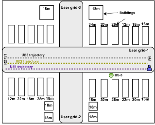
Figure 2: Top view of ‘O1_outdoor scenario’ [12]. Not to scale.

Table II: DeepMIMO dataset and wireless parameters

Parameter	Value
# of BS antennas $(M_{x}\times M_{y}\times M_{z})$	(1$\times$ 8 $\times$ 4)
# of UE antennas {Sub-6; mmWave; THz}	{1; 8; 64}
# of channel paths (strongest gets selected)	3
$\text{P}_{T_{X_{i}}}$ ; Cyclic prefix ratio	1W ; 64
$f_{c}$ {Sub-6; mmWave; THz}	{3.5; 28; 140} GHz
Bandwidth {Sub-6; mmWave; THz}	{10; 100; 1000} MHz
# of OFDM subcarriers; UE speed ; $(v_{s})$	64 ; 10 m/s (36 kmph)

III-C Forecasting Methodology

The UE location is usually correlated with its previous history. This is also justifiable in real-life highway and urban road scenarios. This motivates us to utilize the LSTM as a forecaster. As mentioned earlier, since we generate wireless channel data considering a setting with three UEs, there are a total of 8253 datapoints. We concatenate these datapoints so as to form a temporal sequence. Precisely, we first stack UE3 datapoints followed by UE2 and UE1. An important factor that the LSTM has is that it learns from its history by looking back from the current timestep. In our experiments, based on hyperparameter tuning, we select the lookback to be 15. Thus, LSTM lookbacks 15 time stamps and forecasts either the rate or $|\text{{h}}_{i}|^{2}$ upto $T$-th time slots into the future. We would like to highlight that we use direct multistep ahead forecasting instead of iterative multistep ahead, since in the latter, the error gets accumulated resulting in poor predictions [16]. Once the dataset is formulated, we use first 6000 sequences each of length 15 as a training data (in fig. 2, this is equivalent to the entire data of UE3, UE2, and initial few data points of UE1). The associated label for each sequence would be the next $T$ continuous multistep values. Following the training sequences, we skip some of sequences to avoid data leaking and use following 500 sequences for validation. Lastly, we use 1150 sequences for the test data. Note that this approach is also closely related to the realistic scenario where the BS predicts future behavior based on its recent past and also based on the channel quality of other nearby users (UE2 and UE3 in our case). We built a stacked LSTM forecaster(s), that essentially learns a mapping function between past and future rates, and provides forecasts of the rates and $|\text{{h}}_{i}|^{2}$ to help achieve the objective in eq. (5). The LSTM hyperparameters are summarized in Table III.

In addition to the LSTM based predictor (which performs the best as shown subsequently), we considered a simpler predictor we call current channel prediction and Transformer based forecast. For the current channel prediction, the rate/channel in the current slot is used as the forecast for the remaining slots in the frame. E.g., for the rate predictor, in slot $t$ of a given frame $\hat{R}_{i}[t+1,t]=\cdots=\hat{R}_{i}[T,t]=R_{i}[t]$, where $\hat{R}_{i}[\ell,t]$ is the predicted rate of slot $\ell$ at band $i$ with $t$ denoting when the prediction was made. The Transformer based predictor is based on [17], which has recently received significant attention in the literature. The Transformer hyperparameters are summarized in Table IV.

Table III: Stacked LSTM Hyperparameters

Hyperparameter	Value
learning rate; Batch size; Epochs	0.0001 ; 64 ; 50
Number of layers (Depth)	4 hidden layers + 1 dense layer
Number of LSTM units (Width)	{100, 64, 64, 32}
Dropout	0.4 between hidden layers
Optimizer ; Loss function	Adam ; Mean square error (MSE)
Activation function	ReLU (for hidden layers)

Table IV: Transformer Hyperparameters

Hyperparameter	Value
Batch size; Epochs	256 ; 10
# of Encoder & Decoder layers	4 layers (each)
Dimensionality of the model and its embeddings (d_model)	32
Optimizer ; learning rate ; $\beta_{1}$ ; $\beta_{2}$	AdamW ; 0.0006 ; 0.9 ; 0.95

IV Numerical Results

Table V: Summary of the forecasting errors for the test sequences. Lower the value, better is the prediction.

		Metrics	NRMSE				NMAE
Approach	Bands	Slots	Step 4	Step 3	Step 2	Step 1	Step 4	Step 3	Step 2	Step 1
		LSTM	0.0620	0.0598	0.0541	0.0494	0.0428	0.0388	0.0353	0.0309
	Sub6 GHz	Transformer	0.0615	0.0527	0.0305	0.0181	0.0439	0.0398	0.0231	0.0145
		LSTM	0.1765	0.1717	0.1698	0.1603	0.1366	0.1334	0.1332	0.1247
	mmWave	Transformer	0.2269	0.1984	0.1872	0.1354	0.1723	0.1515	0.1462	0.1005
		LSTM	0.3089	0.3035	0.3020	0.2972	0.2297	0.2225	0.2164	0.2015
I: Rate forecaster	THz	Transformer	0.4263	0.3908	0.3386	0.2200	0.3417	0.3144	0.2657	0.1656
		LSTM	0.4948	0.4623	0.3832	0.2483	0.4948	0.4623	0.3832	0.2483
	Sub6 GHz	Transformer	0.6826	0.5870	0.3798	0.1757	0.3405	0.2950	0.1783	0.0805
		LSTM	1.2307	1.1419	1.0802	1.0222	0.5460	0.5440	0.5420	0.5358
	mmWave	Transformer	1.2126	1.0751	0.8754	0.6849	0.5873	0.5208	0.4264	0.3297
		LSTM	0.7763	0.7702	0.7670	0.6842	0.3974	0.3843	0.3774	0.3767
II: Channel forecaster	THz	Transformer	0.8242	0.8224	0.7758	0.5490	0.4625	0.4509	0.4048	0.2959

For experiments, we used Matlab to generate channels using the ray-tracing scenarios ‘DeepMIMO’ dataset [12], and Keras API [18] with TensorFlow backend to create, the stacked LSTM as a forecaster, while Transformer was built using Pytorch. We consider UE noise figure $=7$ dB, $\sigma_{i}^{2}=$K.Temp.$B_{i}$.UE noise figure, where K is Boltzmann’s constant, and Temp. is temperature $=300$ Kelvin. Switching cost $\nu=0.05$. The power consumed in each band are as per Sec. II-b. To better quantify the prediction errors, we use normalized root mean square error (NRMSE) and normalized mean absolute error (NMAE) as forecaster metric. We compare the proposed stacked LSTM forecaster with the celebrated Transformer model, which uses attention mechanism to capture the context. Hyperparameters were tuned for fair comparison, and the same lookback size of 15 was used for each sequence. Table V summarizes the forecasting errors for both the approaches. We can notice that predictions using the rate forecaster is comparatively more accurate than the channel forecaster. This is intuitive, and due to the fact that the fluctuations in the channel are significantly higher as compared to the rate fluctuations. Furthermore, we can notice that LSTM predictions are much accurate than those of the Transformer, following similar observation in [16].

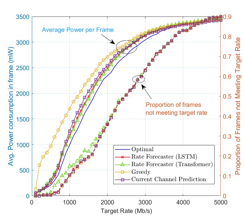
Figure 3: Average Power Consumed vs. Target Rate with rate forecaster.

Although, to the best of our knowledge, there is no existing work with which we can fairly compare the proposed approach, we compare with i) Greedy approach: In this scheme, at the start of each slot, the rates/channels in all bands are estimated. With a possible exception which we will described subsequently, the BS picks the band with the highest rate for that slot. Then, it subtracts the achieved rate in this slot from the target sum rate for the frame in preparation for the next time slot. The exception is if the target sum rate for the frame can be achieved in the current slot by transmitting in a lower-power band. In this case, the BS picks the lowest UE power consumption band which can achieve the sum rate. This approach is named greedy in a sense that the BS always chooses the highest rate band, except when the sum rate in the frame can be satisfied in the current slot with a lower power band. ii) Optimal approach: In this approach, the rates for all slots are known non-causally, and an exhaustive search is done on every frame to find the band assignments which minimizes power consumption at the UE while meeting the target rate.

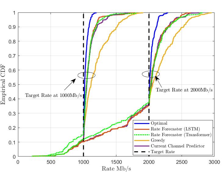
Figure 4: CDF of rates for 1000Mb/s; 2000Mb/s Target Rates.

Fig. 3 shows the plot of average power consumed per frame for various target rates, using different rate forecasters, greedy and optimal approaches. The figure also shows the fraction of frames for which the target rate isn’t met, with the axes labels on the right. Note that the proposed approach with LSTM tracks the optimal approach, and outperforms other considered approaches, except the transformer, in terms of average power consumption. Furthermore, due to the better rate predictions, the LSTM outperforms Transformer for almost all the target rates in terms of the fraction of frames meeting the target rate. Hence, even though the Transformer approach slightly outperforms the LSTM approach for the average power consumption at certain target rates, the significantly higher rate of frames not meeting target makes it less desirable than the LSTM approach. More specifically, with a target rate of 1500 Mb/s, our approach with the LSTM rate forecaster consumes more than 300 mW less than the greedy band selection approach and the current channel predictor consumes about 200 mW less than the greedy approach. Further, the LSTM based approach is within 120 mW of the optimal, non-causal approach. Both the LSTM and optimal approach have the same fraction of frames not meeting the target rate of 1500 Mb/s. Since the fraction of frames which did not meet the target rate are approximately equal for all schemes except the Transformer, the savings in power from the LSTM and current-channel predictor does not come at the expense of a significant statistical reduction in data rates. Further, to help quantify the distribution of rates actually achieved, we plot the CDFs of the rates with the rate forecaster in Fig.4 with target rates as 1000 Mb/s and 2000 Mb/s. The key observation here is that the distribution of rates below the threshold is approximately equal for all approaches except the version with the Transformer-based rate forecaster, which has an appreciably worse CDF when below the target rates.

To better understand the power consumption with the channel forecaster, we plot the average power vs target data rate using this scheme in Fig. 5. From the graph, it is evident that with the channel based forecaster, the gap between the average power of the LSTM scheme and the greedy approach has reduced, and the the current channel predictor performance is very close to that of the LSTM-based channel forecaster. This conclusion is not surprising given the significantly greater accuracy of the rate based forecaster as compared to the channel based forecaster. More generally, the gap between the greedy and optimal band assignments is large, $\sim 500$ mW for a range of rate thresholds, which indicates that this type of optimization can be promising as methods of channel estimation improve in accuracy in the future.

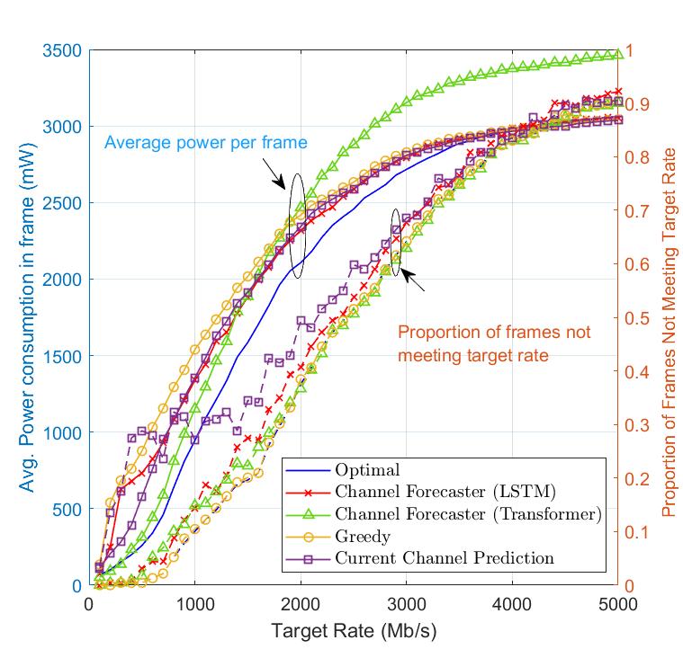
Figure 5: Avg. Power Consumed vs. Target Rate for the Channel forecaster.

V Conclusions

In this work, we propose a novel energy aware band assignment system which reduces the power consumption while also achieving a target rate of at least $M$ average sum rate per frame with $T$ slots. We design Rate forecaster(s) and Channel forecaster(s) which forecasts $T$ direct multistep ahead using a stacked LSTM architecture. Moreover, we propose an iterative rate updating algorithm which updates the target rate based on current rate and future predicted rates in a frame. Research findings shows that the rate forecaster based approach performs better than the channel forecaster. Furthermore, LSTM based predictions outperforms the Transformer-based predictions in terms of NRMSE and NMAE. E.g., with a target rate of 1.5Gb/s, we find that compared to the other approaches, the average power consumption per frame with the proposed approach is $\sim 100$ mW lower than a simple rate forecaster, which uses the current rate as the forecast for future rates, and $\sim 300$ mW lower than a greedy band assignment policy. All of this is obtained while achieving the same distribution of rates below the threshold as the optimal scheme. More generally, we find that a significant power savings (e.g. 500 mW or more) could possibly be obtained by similar band assignment approaches as the ability to forecast channels and rates improves over time, making the framework and analysis introduced in this paper helpful in improving the energy efficient operation of future wireless networks.

References

- [1] S. Tripathi, N. V. Sabu, A. K. Gupta, and H. S. Dhillon, “Millimeter-wave and Terahertz spectrum for 6G wireless,” arXiv preprint arXiv:2102.10267, 2021.
- [2] H. Elayan, O. Amin, B. Shihada, R. M. Shubair, and M.-S. Alouini, “Terahertz band: The last piece of RF spectrum puzzle for communication systems,” IEEE Open J. Commun. Soc., vol. 1, pp. 1–32, 2020.
- [3] O. Semiari, W. Saad, M. Bennis, and M. Debbah, “Integrated millimeter wave and sub-6 GHz wireless networks: A roadmap for joint mobile broadband and ultra-reliable low-latency communications,” IEEE Wireless Commun., vol. 26, no. 2, pp. 109–115, Apr. 2019.
- [4] A. S. Cacciapuoti, K. Sankhe, M. Caleffi, and K. R. Chowdhury, “Beyond 5G: THz-based medium access protocol for mobile heterogeneous networks,” IEEE Commun. Mag., vol. 56, no. 6, pp. 110–115, 2018.
- [5] S. Sur, I. Pefkianakis, X. Zhang, and K.-H. Kim, “Wifi-assisted 60 GHz wireless networks,” in Proc. of the 23rd ACM MOBICOM, New York, USA, 2017, pp. 28–40.
- [6] D. Burghal and A. F. Molisch, “Rate and outage probability in dual band systems with prediction-based band switching,” IEEE Wireless Commun. Lett., vol. 7, no. 5, pp. 872–875, Oct 2018.
- [7] D. Burghal, R. Wang, A. Alghafis, and A. F. Molisch, “Supervised ML solution for band assignment in dual-band systems with omnidirectional and directional antennas,” IEEE Trans. Wireless Commun., vol. 21, no. 9, pp. 7550–7565, 2022.
- [8] F. B. Mismar, A. Alammouri, A. Alkhateeb, J. G. Andrews, and B. L. Evans, “Deep learning predictive band switching in wireless networks,” IEEE Trans. Wireless Commun., vol. 20, no. 1, pp. 96–109, 2021.
- [9] G. Fontanesi, A. Zhu, and H. Ahmadi, “Deep reinforcement learning for dynamic band switch in cellular-connected UAV,” in Proc. of IEEE 94th VTC-Fall, Sep. 2021.
- [10] P. Skrimponis and et. al, “Power consumption analysis for mobile mmwave and sub-THz receivers,” in 6G Wireless Summit, 2020.
- [11] B. Soni, S. Govindasamy, and D. K. Patel, “Deep learning aided energy efficient band assignment in multiband heterogeneous networks,” in Proc. of 20th IEEE CCNC, 2023, pp. 690–691.
- [12] A. Alkhateeb, “DeepMIMO: A generic deep learning dataset for millimeter wave and massive MIMO applications,” CoRR, vol. abs/1902.06435, 2019.
- [13] S. Cui, A. Goldsmith, and A. Bahai, “Energy-constrained modulation optimization,” IEEE Trans. Wireless Commun., vol. 4, no. 5, pp. 2349–2360, 2005.
- [14] Y. Li, B. Bakkaloglu, and C. Chakrabarti, “A system level energy model and energy-quality evaluation for integrated transceiver front-ends,” IEEE Trans. Very Large Scale Integr. (VLSI) Syst., vol. 15, no. 1, pp. 90–103, 2007.
- [15] W. B. Abbas, F. Gomez-Cuba, and M. Zorzi, “Millimeter wave receiver efficiency: A comprehensive comparison of beamforming schemes with low resolution adcs,” IEEE Trans. Wireless Commun., vol. 16, no. 12, pp. 8131–8146, 2017.
- [16] A. Zeng, M. Chen, L. Zhang, and Q. Xu, “Are transformers effective for time series forecasting?” Proceedings of the AAAI Conference on Artificial Intelligence, 2023.
- [17] A. Vaswani and et. al, “Attention is all you need,” Advances in Neural Information Processing Systems, vol. 30, 2017.
- [18] F. Chollet et al., “Keras,” Available: https://github.com/fchollet/keras, 2015.