An inflation model for massive primordial black holes to interpret the JWST observations

Abstract

The first observations of the James Webb Space Telescope (JWST) have identified six massive galaxy candidates with the stellar masses $M_{\ast}\gtrsim 10^{10}\,M_{\odot}$ at high redshifts $7.4\lesssim z\lesssim 9.1$, with two most massive high-$z$ objects having the cumulative comoving number densities $n_{\rm G}$ up to $1.6\times 10^{-5}\,{\rm Mpc}^{-3}$. The presence of such massive sources in the early universe challenges the standard $\Lambda$CDM model since the needed star formation efficiency is unrealistically high. This tension can be alleviated via the accretion of massive primordial black holes (PBHs). In this work, with the updated data from the first JWST observations, we find that the PBHs with mass $10^{8}\,M_{\odot}\lesssim M_{\rm PBH}\lesssim 10^{11}\,M_{\odot}$ can act as the seeds of extremely massive galaxies even with a low abundance $10^{-7}\lesssim f_{\rm PBH}\lesssim 10^{-3}$. We construct an ultraslow-roll inflation model and investigate its possibility of producing the required PBHs. We explore the model in two cases, depending on whether there is a perfect plateau on the inflaton potential. If the plateau is allowed to incline slightly, our model can produce the PBHs that cover the required PBH mass and abundance range to explain the JWST data.

1 Introduction

Owing to the excellent performance of the James Webb Space Telescope (JWST), we can take a deeper look at the end of the cosmic dark ages. So far, several bright galaxy candidates at very high redshifts have already been identified by the JWST [1, 2, 3, 4, 5, 6, 7, 8]. Intriguingly, a group of massive galaxy candidates at redshifts $6.5\lesssim z\lesssim 9.1$ were detected via the JWST Cosmic Evolution Early Release Science (CEERS) program, with the inferred stellar masses $M_{\ast}\gtrsim 10^{9}\,M_{\odot}$ ($M_{\odot}=1.99\times 10^{30}$ kg is the solar mass) [6]. Among them, there are six sources with the stellar masses $M_{\ast}\gtrsim 10^{10}M_{\odot}$ at $7.4\lesssim z\lesssim 9.1$ [6], including two most extreme galaxies with halos that have the cumulative comoving number densities $n_{\rm G}\lesssim 1.6\times 10^{-5}\,{\rm Mpc}^{-3}$ [9]. These six massive galaxies imply the star formation efficiency $\epsilon=0.99$ at $z\approx 9$ and $\epsilon=0.84$ at $z\approx 7.5$ [9], which seems physically implausible [10, 11]. Even if considering the $1\sigma$ error, such a high $\epsilon$ is still hard to reach. This apparent difficulty brings challenges to the theoretical framework of early structure formation and even to the standard $\Lambda$CDM model [9, 12, 13]. As a result, various mechanisms have been proposed to make the $\Lambda$CDM model compatible with the JWST observations [14, 15, 16, 17, 18, 19], such as weakening the dust attenuation in high-$z$ galaxies [20, 21] and enhancing the effectiveness of the star formation efficiency [22]. Recently, it has also been reported that such early massive galaxies may be induced by the accretion of massive primordial black holes (PBHs) [23, 24].

The study on PBHs dates back to half a century ago [25, 26] and is receiving increasing interest in recent years. The basic motivations are manifold. For instance, the merger of binary PBHs can emit gravitational waves detected by the LIGO/Virgo/KAGRA collaboration [27, 28, 29]. Also, the first-order scalar perturbations that generate PBHs can simultaneously serve as the source of the second-order scalar-induced gravitational waves [30, 31, 32]. More importantly, PBH is a natural and promising candidate of dark matter (DM) in certain mass ranges [33]. Generally speaking, there are two ways for PBHs to induce cosmic structure: the Poisson effect [34, 35] and the seed effect [36, 37, 38]. If PBHs occupy a major portion of DM, the Poisson effect dominates on all scales. On the contrary, if PBHs only contribute a small fraction to DM, the seed effect dominates on small scales.

The PBH abundance $f_{\rm PBH}$ is defined as its proportion in DM today, and PBH can be considered an effective DM candidate if $f_{\rm PBH}\gtrsim 0.1$. Assuming that the mass distribution of PBHs is monochromatic (i.e., all PBHs possess the same mass), $f_{\rm PBH}$ is constrained by various astronomical observations, especially in the mass range $M_{\rm PBH}\gtrsim M_{\odot}$ [39, 40, 41, 38]. However, a mass window from $10^{-17}M_{\odot}$ (asteroid mass range) to $10^{-13}M_{\odot}$ (sub-lunar mass range) is still completely open. If so, the Poisson effect caused by supermassive PBHs is trivial [17]. Then, the PBH explanation is farfetched if the massive galaxies in the early cosmic history are abundant. Fortunately, these constraints are relatively weak for the seed effect [23, 17], and PBHs are still substantial in accelerating early massive galaxies. In this respect, the tension between the JWST observations and the $\Lambda$CDM model would be alleviated to a great extent [23, 24].

In the radiation-dominated era of the early universe, if the density contrast of the radiation field exceeds some threshold, the overdense region can directly collapse to PBHs at the horizon reentry after cosmic inflation. The usual single-field slow-roll (SR) inflation models are successful in explaining the large-scale perturbations measured by the anisotropies of the cosmic microwave background (CMB) [42], but cannot generate a sufficiently large density contrast on small scales. Therefore, many new types of inflation models have been constructed, commonly known as the ultraslow-roll (USR) inflation, which usually contains a plateau or saddle point on the single- or multi-field background inflaton potential $V_{\rm b}$, leading the inflaton to evolve extremely slowly thereby. During the USR stage, the density contrast of the radiation field can be significantly enhanced on small scales, inducing the PBHs with desirable mass and abundance.

In general, there are two mechanisms to implement the USR conditions, which are the (near-)inflection point on $V_{\rm b}$ [43, 44, 45, 46, 47, 48, 49, 50, 51, 52, 53, 54] and the independent bumps or dips on $V_{\rm b}$ [55, 56, 57, 58, 59, 60, 61, 32]. In this paper, we adopt the second method and suggest an antisymmetric form for the perturbation $\delta V$ on $V_{\rm b}$ to realize the USR inflation. Then, we explore the possibilities to explain the JWST observations via the PBHs generated from our model. Based on the updated data from the first JWST observations [6, 9], we find that our model can effectively reconcile the tension between the JWST observations and the $\Lambda$CDM model through the seed effect for the PBHs with mass $10^{8}\,M_{\odot}\lesssim M_{\rm PBH}\lesssim 10^{11}\,M_{\odot}$, even if their abundance is merely $10^{-7}\lesssim f_{\rm PBH}\lesssim 10^{-3}$. In contrast, the Poisson effect can be convincingly ruled out.

This paper is organized as follows. In section 2, the calculation of the PBH mass $M_{\rm PBH}$ and abundance $f_{\rm PBH}$ is briefly reviewed. In section 3, we study the Poisson and seed effects and calculate the required ranges of $M_{\rm PBH}$ and $f_{\rm PBH}$ to explain the JWST observations based on the updated data. In sections 4 and 5, we construct a USR inflation model and discuss it in two cases to explore the influences from the profile of the perturbation. Finally, we conclude in section 6. We work in the natural system of units and set $c=\hbar=k_{\rm B}=1$.

2 PBH mass and abundance

In this section, we investigate the power spectrum of primordial curvature perturbation within the framework of the single-field inflation model and calculate the PBH abundance in peak theory in detail.

2.1 Power spectrum

In the standard single-field inflation model, the scalar inflaton field $\phi$ is minimally coupled to gravity, and the corresponding action reads

$$S=\int{\rm d}^{4}x\,\sqrt{-g}\left[\frac{m_{\rm P}^{2}}{2}R-\frac{1}{2}\partial_{\mu}\phi\partial^{\mu}\phi-V(\phi)\right],$$

where $V(\phi)$ is the inflaton potential, $R$ is the Ricci scalar, and $m_{\rm P}=1/\sqrt{8\pi G}$ is the reduced Planck mass, respectively. To measure the cosmic expansion more conveniently, we utilize the number of $e$-folds $N$ as a new time variable, defined as ${\rm d}N=H\,{\rm d}t={\rm d}\ln a$, where $a=e^{N}$ is the scale factor, and $H=\dot{a}/a$ is the Hubble expansion rate. To address the flatness and horizon problems in the standard hot Big Bang model, a quasi-de Sitter expansion period lasting at least 60–70 $e$-folds is required. In the following, $N_{\ast}\sim 20$ is chosen to represent the number of $e$-folds for the CMB pivot scale $k_{\ast}=0.05\,{\rm Mpc}^{-1}$ at its horizon-exit [42].

To characterize the motion of the inflaton on its potential, two useful parameters can be introduced as

$$\varepsilon =-\frac{\dot{H}}{H^{2}}=\frac{\phi_{,N}^{2}}{2m_{\rm P}^{2}},$$

$$\eta =-\frac{\ddot{\phi}}{H\dot{\phi}}=\frac{\phi_{,N}^{2}}{2m_{\rm P}^{2}}-\frac{\phi_{,NN}}{\phi_{,N}}.$$

In the usual SR inflation, $\varepsilon,|\eta|\ll 1$ and are thus named as the SR parameters. However, in the USR stage, both SR conditions can be broken, and their values may be greatly changed, leaving significant influences on cosmic evolution and PBH abundance. In terms of the SR parameters, the evolution of $\phi$ is depicted by the Klein–Gordon equation as

$$\phi_{,NN}+(3-\varepsilon)\phi_{,N}+\frac{1}{H^{2}}V_{,\phi}=0,$$

and the Friedmann equation for cosmic expansion reads

$$H^{2}=\frac{V}{(3-\varepsilon)m^{2}_{\rm P}}.$$

Now, we consider the perturbations on the background universe. Since the vector and tensor perturbations are irrelevant to the production of PBHs, we focus on the scalar perturbation $\Phi$. Neglecting anisotropic stress, the perturbed metric in the conformal Newtonian gauge can be expressed as

$${\rm d}s^{2}=-(1+2\Phi)\,{\rm d}t^{2}+a^{2}(t)(1-2\Phi)\delta_{ij}\,{\rm d}x^{i}{\rm d}x^{j}.$$

A more useful and gauge-invariant primordial curvature perturbation ${\cal R}$ can be further defined as

$${\cal R}=\Phi+\frac{H}{\dot{\phi}}\delta\phi=\Phi+\frac{\delta\phi}{\phi_{,N}},$$

and its equation of motion in the Fourier space is the Mukhanov–Sasaki equation [62, 63],

$${\cal R}_{k,NN}+(3+\varepsilon-2\eta){\cal R}_{k,N}+\frac{k^{2}}{H^{2}e^{2N}}{\cal R}_{k}=0.$$

To obtain the PBH mass and abundance, we need to calculate the two-point correlation function of ${\cal R}$, or its power spectrum in the Fourier space. Usually, the dimensionless power spectrum ${\cal P}_{\cal R}(k)$ is introduced as

$${\cal P}_{\cal R}(k)=\left.\frac{k^{3}}{2\pi^{2}}\left|{\cal R}_{k}\right|^{2}\right|_{k\ll aH}.$$

In the SR inflation, ${\cal R}_{k}$ becomes almost frozen once the scale $k$ crosses the horizon, so ${\cal P}_{\cal R}(k)$ can be effectively calculated at $k=aH$. However, in the USR inflation, ${\cal R}_{k}$ can still significantly evolve after the horizon-exit, so ${\cal P}_{\cal R}(k)$ must be evaluated at the end of inflation when $k\ll aH$. On the large scales around the CMB pivot scale $k_{\ast}$, ${\cal P}_{\cal R}(k)$ can usually be formulated in a nearly scale-invariant power-law form as

$${\cal P}_{\cal R}(k)=A_{\rm s}\left(\frac{k}{k_{\ast}}\right)^{n_{\rm s}-1},$$

with the central values of the scalar spectral index $n_{\rm s}=0.965$ and the amplitude $A_{\rm s}=2.10\times 10^{-9}$ [64].

In the radiation-dominated era, ${\cal P}_{\cal R}(k)$ is proportional to the dimensionless power spectrum of primordial density contrast ${\cal P}_{\delta}(k)$ [65],

$${\cal P}_{\delta}(k)=\frac{16}{81}\left(\frac{k}{aH}\right)^{4}{\cal P}_{\cal R}(k).$$

To avoid the non-differentiability and divergence in the large-$k$ limit of the radiation field, the density contrast $\delta$ needs to be smoothed on a large scale, usually taken as $R=1/(aH)$. This can be realized by a convolution of $\delta$ as $\delta({\bf x},R)=\int{\rm d}^{3}x^{\prime}\,W({\bf x}-{\bf x}^{\prime},R)\delta({\bf x}^{\prime})$, with $W({\bf x},R)$ being the window function. Below, we choose Gaussian window function as $\widetilde{W}(k,R)=e^{-k^{2}R^{2}/2}$ in the Fourier space, meaning that $W({\bf x},R)=e^{-{x^{2}}/({2R^{2}})}/V(R)$ in real space, and the volume $V(R)=(\sqrt{2\pi}R)^{3}$ is the normalization factor. Altogether, the variance of the smoothed density contrast on the scale $R$ is given by

$$\sigma_{\delta}^{2}(R)=\langle\delta^{2}({\bf x},R)\rangle=\int_{0}^{\infty}\frac{{\rm d}k}{k}\,\widetilde{W}^{2}(k,R){\cal P}_{\delta}(k),$$

where $\langle\cdots\rangle$ denotes the ensemble average, and we have used the fact $\langle\delta({\bf x},R)\rangle=0$ for the Gaussian random field. Moreover, because of the homogeneity and isotropy of the background universe, $\sigma_{\delta}^{2}(R)$ is independent of a special position ${\bf x}$. Similarly, the $i$-th spectral moment of the smoothed density contrast is defined as

$$\sigma_{i}^{2}(R) =\int_{0}^{\infty}\frac{{\rm d}k}{k}\,k^{2i}\widetilde{W}^{2}(k,R){\cal P}_{\delta}(k)=\frac{16}{81}\int_{0}^{\infty}\frac{{\rm d}k}{k}\,k^{2i}\widetilde{W}^{2}(k,R)(kR)^{4}{\cal P}_{{\cal R}}(k),$$

where $i=0,1,2,...$, and $\sigma_{0}=\sigma_{\delta}$ naturally.

2.2 PBH mass and abundance

In the Carr–Hawking collapse model [66], with the conservation of entropy in the adiabatic cosmic expansion taken into account, the PBH mass $M_{\rm PBH}$ is [39]

$$\frac{M_{\rm PBH}}{M_{\odot}}=1.13\times 10^{15}\left(\frac{\kappa}{0.2}\right)\left(\frac{g_{\ast}}{106.75}\right)^{-1/6}\left(\frac{k_{\ast}}{k_{{\rm PBH}}}\right)^{2},$$ (2.1)

where $\kappa$ is the efficiency of collapse, $k_{{\rm PBH}}=1/R$ is the wave number of the PBH at the horizon-exit, and $g_{\ast}$ is the effective relativistic degree of freedom for energy density at the PBH formation, respectively. Below, we set $\kappa=0.2$ and $g_{\ast}=106.75$ [67]. From eq. (2.1), all spectral moments $\sigma_{i}(R)$ can be reexpressed in terms of the PBH mass as $\sigma_{i}(M_{\rm PBH})$.

For the monochromatic PBH mass distribution, the peak theory is the most general method to calculate the PBH mass fraction $\beta_{\rm PBH}$ at the moment of its formation [68], in which the peak value $\nu=\delta/\sigma_{\delta}$ is the relative density contrast. The threshold of $\nu$ can be expressed as $\nu_{\rm c}=\delta_{\rm c}/\sigma_{\delta}$, where $\delta_{\rm c}$ is the most influential factor in calculating $\beta_{\rm PBH}$, and it depends on the equation of state of the cosmic media and many other ingredients [69, 70, 71, 72, 73, 74, 75, 76, 77, 78, 79]. Below, we follow ref. [73] and adopt the most accepted value as $\delta_{\rm c}=0.414$.

In peak theory, the number density of peaks is $n({\bf r})=\sum_{p}\delta_{\rm D}({\bf r}-{\bf r}_{p})$, with $\delta_{\rm D}$ being the Dirac function, and ${\bf r}_{p}$ denoting the position where the density contrast $\delta$ has a local maximum. To determine this maximum condition, a ten-dimensional joint probability distribution function (PDF) $P(\{y_{i}\})$ of Gaussian variables as

$$P(\{y_{i}\})=\frac{\exp\big{(}\frac{1}{2}\sum_{ij}\Delta y_{i}{\cal M}^{-1}_{ij}\Delta y_{j}\big{)}}{\sqrt{(2\pi)^{10}\det{\cal M}}}$$

needs to be addressed, where ${\cal M}$ is the covariance matrix and $\Delta y_{i}=y_{i}-\langle y_{i}\rangle$, with $y_{1}=\delta$, $y_{2}=\partial_{1}\delta$, …, $y_{5}=\partial_{1}\partial_{1}\delta$, …, and $y_{10}=\partial_{2}\partial_{3}\delta$. By a series of dimensional reduction, the ten-dimensional joint PDF $P(\{y_{i}\})$ can be eventually reduced to a one-dimensional conditional PDF $P(\nu)$ [68]. From $P(\nu)$, the PBH mass fraction can be obtained in an integral form as

$$\beta_{\rm PBH}=\frac{1}{\sqrt{2\pi}}\left(\frac{R\sigma_{2}}{\sqrt{3}\sigma_{1}}\right)^{3}\int_{\nu_{\rm c}}^{\infty}G(\gamma,\nu)e^{-\nu^{2}/2}\,{\rm d}\nu,$$

where $\gamma=\sigma_{1}^{2}/(\sigma_{\delta}\sigma_{2})$ contains information of the profile of the density contrast $\delta$.

The constraint condition that the peak position corresponds to the local maximum of $\delta$ is implicitly encoded in the $G(\gamma,\nu)$ function, which is rather complicated. Consequently, a convenient approximation (i.e., $\nu>1$ and $\gamma\approx 1$) introduced by Green, Liddle, Malik, and Sasaki in ref. [65] is usually consulted in peak theory. In this approximation, there remain only two independent spectral moments $\sigma_{\delta}$ and $\sigma_{1}$, and the PBH mass fraction can be analytically expressed as

$$\beta_{\rm PBH}=\frac{1}{\sqrt{2\pi}}\left(\frac{\sigma_{1}}{\sqrt{3}\sigma_{\delta}}\right)^{3}(\nu_{\rm c}^{2}-1)e^{-\nu_{\rm c}^{2}/2}.$$

For other kinds of approximation at different levels of peak theory, see refs. [61, 80, 81, 82, 32].

For the massive PBHs not evaporated yet today, the abundance $f_{\rm PBH}$ is naturally proportional to the mass fraction $\beta_{\rm PBH}$ [39],

$$f_{\rm PBH}=1.68\times 10^{8}\left(\frac{M_{\rm PBH}}{M_{\odot}}\right)^{-1/2}\beta_{\rm PBH}.$$

It should be noted that here we have neglected the evolution of PBHs (e.g., radiation, accretion, and merger), so when considering the accretion of PBHs to produce massive galaxies in section 3, we must assume that the bound region will not drop into the horizon of PBHs. Thus, we eventually achieve the PBH abundance $f_{\rm PBH}$ in peak theory.

3 Early massive galaxies generated by supermassive PBHs

In this section, we briefly introduce the Poisson and seed effects and then discuss the ranges of the PBH mass and abundance required to explain the JWST observations.

3.1 Poisson and seed effects

Massive PBHs can behave as the source of fluctuations on a mass scale $M_{\rm B}$ through the Poisson effect [34, 35] or the seed effect [36, 37, 38]. The former provides an initial density fluctuation via the $\sqrt{N}$ fluctuation in the number of black holes collectively [36], while the latter provides the fluctuation via the Coulomb effect of an individual black hole [37]. Both fluctuations then grow through gravitational instability to bind regions [38].

With the monochromatic PBH mass distribution [38], the initial fluctuations in the matter density of the Poisson and seed effects are

$$\delta_{\rm ini}\approx\left\{\begin{aligned} &\sqrt{\frac{M_{\rm PBH}f_{\rm PBH}}{M_{\rm B}}}\quad(\text{Poisson effect}),\\ &\frac{M_{\rm PBH}}{M_{\rm B}}\qquad\qquad\,(\text{seed effect}).\end{aligned}\right.$$

The above semi-analytical approach is accurate in two limits: $f_{\rm PBH}\to 1$ for the Poisson effect and $f_{\rm PBH}\to 0$ for the seed effect, respectively. For the complex situation with $10^{-4}\lesssim f_{\rm PBH}\lesssim 10^{-1}$, in which the two effects interplay, the $N$-body simulation is needed [83, 84]. Nonetheless, due to the various constraints on $f_{\rm PBH}$ [39, 40, 41, 38], our research will focus on the seed effect with $f_{\rm PBH}\ll 1$, so the semi-analytical model is sufficient (to be explained in more detail in section 3.2).

Then, we briefly distinguish the dominant mechanism on each mass scale in two different ways. First, in view of the competition from other seeds, a region of mass $M_{\rm B}$ may contain more than one black hole. However, the seed effect is provided by a PBH growing in isolation, so the mass $M_{\rm B}$ bound by a single seed should never exceed $M_{\rm PBH}/f_{\rm PBH}$. Therefore, the bound region has a critical mass $M_{\rm c}$ as

$$M_{\rm c}\approx\frac{M_{\rm PBH}}{f_{\rm PBH}}.$$ (3.1)

As a result, when $M_{\rm B}\gtrsim M_{\rm c}$, the Poisson effect dominates; when $M_{\rm B}\lesssim M_{\rm c}$, the seed effect dominates.

Second, since each PBH is surrounded by the high-density radiation field at its formation, the $\sqrt{N}$ fluctuation is not initially associated with total density. As the radiation density drops rapidly, a fluctuation in total density can definitely form. In other words, the $\sqrt{N}$ fluctuation is frozen during the radiation-dominated era but grows in the matter-dominated era, and the mass $M_{\rm B}$ binding at the redshift $z_{\rm B}$ is [38]

$$M_{\rm B}\approx\left\{\begin{aligned} &\frac{M_{\rm PBH}f_{\rm PBH}}{[(1+z_{\rm B})a_{\rm eq}]^{2}}\quad(\text{Poisson effect}),\\ &\frac{M_{\rm PBH}}{(1+z_{\rm B})a_{\rm eq}}\qquad(\text{seed effect}),\end{aligned}\right.$$ (3.2)

where $a_{\rm eq}=1/(1+z_{\rm eq})$ is the scale factor at the matter–radiation equality with $z_{\rm eq}\approx 3400$. From eqs. (3.1) and (3.2), ignoring the observational constraints on $f_{\rm PBH}$, one can derive the critical abundance in terms of the mass binding redshift $z_{\rm B}$ as

$$f_{\rm c}\approx(1+z_{\rm B})a_{\rm eq}.$$ (3.3)

Hence, when $f_{\rm PBH}\gtrsim f_{\rm c}$, the Poisson effect dominates; otherwise, the seed effect dominates.

3.2 PBH mass and abundance required to explain the JWST observations

As mentioned above, via the acceleration by supermassive PBHs, the identified galaxy candidates in the first observations of the JWST CEERS program with incredible masses at high redshifts would reconcile with the standard $\Lambda$CDM model. In the following, we will base on the conclusions in ref. [6] and ideally determine the ranges of the PBH mass and abundance that can explain these observations.

We start from the star formation efficiency $\epsilon$,

$$\epsilon=\frac{M_{\ast}}{f_{\rm b}M_{\rm halo}},$$ (3.4)

where $M_{\rm halo}$ is the halo mass, and $f_{\rm b}=\Omega_{\rm b}/\Omega_{\rm m}$ is the cosmic average fraction of baryons in matter, with $\Omega_{\rm b}=0.0493$ and $\Omega_{\rm m}=0.3153$ [64]. Assuming that the halo mass $M_{\rm halo}\sim M_{\rm B}$ and the galaxy redshift $z\sim z_{\rm B}$, for the Poisson effect, from eq. (3.2), we have

$$M_{\rm halo}\approx\frac{M_{\rm PBH}f_{\rm PBH}}{[(1+z)a_{\rm eq}]^{2}}.$$ (3.5)

To explain the JWST observations on all scales by the Poisson effect, we take $M_{\ast}=10^{10}\,M_{\odot}$, with $z=7.5$ and $9$. From eqs. (3.4) and (3.5), we roughly have

$$M_{\rm PBH}f_{\rm PBH}\epsilon \gtrsim 4.0\times 10^{5}\,M_{\odot}\quad(z=7.5),$$

$$M_{\rm PBH}f_{\rm PBH}\epsilon \gtrsim 5.6\times 10^{5}\,M_{\odot}\quad(z=9).$$

Since both $f_{\rm PBH}$ and $\epsilon$ should be less than 1, we have $M_{\rm PBH}\gtrsim 10^{5}\,M_{\odot}$.

However, if the primordial density fluctuations are Gaussian, such PBH mass is strongly constrained by the observations from the CMB $\mu$-distortion [39]. The constraints can be mitigated to a certain extent if the Gaussian assumption is relaxed [85]. Nevertheless, there are still several other constraints to be considered. First, the PBHs with mass $M_{\rm PBH}>10^{11}\,M_{\odot}$ have already been excluded due to the non-detection except for Phoenix A [86]. Second, besides the $\mu$-distortion constraint, the PBHs with $M_{\rm PBH}\gtrsim 10^{5}\,M_{\odot}$ also have relatively weaker constraint from the X-ray binaries [40], the infall of PBHs into the Galactic center by dynamical friction [41], and the large-scale structure statistics [38], which together require $f_{\rm PBH}\lesssim 10^{-4}$–$10^{-3}$ for $M_{\rm PBH}\sim 10^{5}$–$10^{11}M_{\odot}$. Furthermore, according to the high-$z$ Lyman-$\alpha$ forest data [87], the PBHs with $M_{\rm PBH}f_{\rm PBH}\gtrsim 170\,M_{\odot}$ and $f_{\rm PBH}>0.05$ have already been ruled out, meaning that the supermassive PBHs that can provide the Poisson effect are strongly disfavored. The above constraints make it almost impossible to explain the JWST observations via the Poisson effect.

Fortunately, the seed effect, which works on small scales, still possesses the potential to explain the JWST observations. Here, we consider two most massive high-$z$ objects, Galaxies 35300 and 38094 (G1 and G2 for short hereafter), with their stellar masses $M_{\ast}$ and redshifts $z$ as [6]

$$M_{\ast} \approx 2.5\times 10^{10}M_{\odot},\quad z\approx 9.1\quad\text{(G1)},$$

$$M_{\ast} \approx 7.8\times 10^{10}M_{\odot},\quad z\approx 7.5\quad\text{(G2)}.$$

On the one hand, from eq. (3.3), the seed effect is likely to dominate if $f_{\rm PBH}\lesssim(1+z)a_{\rm eq}$. Taking into account the redshifts of G1 and G2, we approximately obtain the dominant region for the seed effect as

$$f_{\rm PBH}\lesssim 3\times 10^{-3}.$$ (3.6)

This result is generally consistent with the constraints from the X-ray binaries [40], the infall of PBHs into the Galactic center by dynamical friction [41], and the large-scale structure statistics [38]. On the other hand, due to the nonlinear dynamics around the PBH-seeded halo [84, 23], the Lyman-$\alpha$ forest constraint [87] can be weakened on small scales, where each halo contains less than one PBH on average. Altogether, these factors necessitate further analysis on the seed effect.

From eq. (3.2), the mass of the observed galaxies seeded by the PBHs growing in isolation is [38]

$$M_{\rm halo}\approx\frac{M_{\rm PBH}}{(1+z)a_{\rm eq}}.$$ (3.7)

As the JWST data in ref. [6] have been updated, we derive two idealized conditions following the methods in ref. [23].

First, the cosmic comoving number density of PBHs is

$$\overline{n}_{\rm PBH}=\frac{3H_{0}^{2}(\Omega_{\rm m}-\Omega_{\rm b})}{8\pi G}\frac{f_{\rm PBH}}{M_{\rm PBH}}\approx 3.25\times 10^{10}\frac{f_{\rm PBH}}{M_{\rm PBH}}M_{\odot}\,{\rm Mpc}^{-3},$$

where $H_{0}=67.36~{}{\rm km}~{}{\rm s}^{-1}~{}{\rm Mpc}^{-1}$ is the Hubble constant [64]. Obviously, $\overline{n}_{\rm PBH}$ must be larger than the comoving number densities $n_{\rm G}$ of G1 and G2. Here, $n_{\rm G}\lesssim 1.6\times 10^{-5}\,{\rm Mpc}^{-3}$ corresponds to $\epsilon=1$ [9], so that we can have the strictest constraint on $f_{\rm PBH}$, otherwise $f_{\rm PBH}$ can be too small to make sense. Thus, we have

$$\frac{M_{\rm PBH}}{f_{\rm PBH}}\lesssim 2.0\times 10^{15}M_{\odot}.$$ (3.8)

Second, the relation $\epsilon f_{\rm b}M_{\rm halo}=M_{\ast}$ is to ensure that the PBH-seeded halos have enough gas to form stars. From eq. (3.7), the PBH mass should satisfy

$$M_{\rm PBH} \approx\frac{M_{\ast}(1+z)a_{\rm eq}}{f_{\rm b}\epsilon}\approx\left\{\begin{aligned} &\frac{4.8\times 10^{8}}{\epsilon}M_{\odot}\quad(\text{G1}),\\ &\frac{1.3\times 10^{9}}{\epsilon}M_{\odot}\quad(\text{G2}).\end{aligned}\right.$$ (3.9)

According to eqs. (3.8) and (3.9), the seed effect can explain the JWST observations in a relatively less extreme range of PBH mass $M_{\rm PBH}$ and abundance $f_{\rm PBH}$.

4 USR inflation model

In this section, we construct a specific USR inflation model to generate the PBHs with the required mass and abundance to explain the JWST observations.

In this work, we follow the method in refs. [60, 61, 32] and consider an antisymmetric perturbation $\delta V$ on the background inflaton potential $V_{\rm b}$. There are several advantages for such a construction. For example, $\delta V$ can be connected to $V_{\rm b}$ very smoothly on both sides of the USR region, and the inflaton can definitely surmount the perturbation. Also, the USR stage can be separately studied from the SR stage without spoiling the nearly scale-invariant power spectrum ${\cal P}_{\cal R}(k)$ on large scales. Moreover, there is no modulated oscillation in ${\cal P}_{\cal R}(k)$, naturally avoiding the overproduction of tiny PBHs.

First, we choose the Kachru–Kallosh–Linde–Trivedi potential [88] as the background inflaton potential $V_{\rm b}(\phi)$,

$$V_{\rm b}(\phi)=V_{0}\frac{\phi^{2}}{\phi^{2}+(m_{\rm P}/2)^{2}},$$

where the energy scale of inflation can be taken as $V_{0}/m_{\rm P}^{4}=10^{-10}$. Furthermore, we set the initial conditions for inflation as $\phi/m_{\rm P}=3.30$ and $\phi_{,N}/m_{\rm P}=-0.0137$, such that ${\cal P}_{\cal R}(k)$ has a nearly power-law form on large scales, with the scalar spectral index $n_{\rm s}=0.9591$ at the CMB pivot scale $k_{\ast}=0.05\,{\rm Mpc}^{-1}$. In addition, the tensor-to-scalar $r=0.00322$ is relatively small. Thus, both $n_{\rm s}$ and $r$ satisfy the CMB bounds at $2\sigma$ confidence level [64].

Next, we impose the antisymmetric perturbation $\delta V$ on $V_{\rm b}$,

$$\delta V(\phi)=-A(\phi-\phi_{0})F\left(\frac{\phi-\phi_{0}}{\sqrt{2}\sigma}\right),$$

where $F$ is an even function satisfying $\lim\limits_{x\to\infty}xF(x)=0$. There are three parameters in our model: $A$, $\phi_{0}$, and $\sigma$, characterizing the slope, position, and width of $\delta V$, respectively. As long as $A$ is close to $V_{\rm b,\phi}(\phi_{0})$, a plateau can be created around $\phi_{0}$.

The specific form of the $F$ function is not unique, and we choose Gaussian form in this paper,

$$\delta V(\phi)=-A(\phi-\phi_{0})\exp\left[-\frac{(\phi-\phi_{0})^{2}}{2\sigma^{2}}\right].$$

Other types of the $F$ function have also been investigated in refs. [60, 61], such as Lorentzian form. However, Lorentzian form usually converges more slowly than Gaussian form with the same model parameters, so it always reduces $n_{\rm s}$ too much if $M_{\rm PBH}\gtrsim 10^{3}$–$10^{4}\,M_{\odot}$, which is not consistent with the CMB constraints. Hence, we will only discuss Gaussian form in the following section.

Altogether, the total inflaton potential reads

$$V(\phi)=V_{\rm b}(\phi)+\delta V(\phi).$$

When the inflaton enters the USR stage, it varies extremely slowly and thus significantly enhances the power spectrum and the PBH abundance.

5 PBHs from the USR inflation models

In the inflaton potential constructed above, there are three model parameters in total. Since only two constraints from the PBH mass $M_{\rm PBH}$ and abundance $f_{\rm PBH}$ are imposed on them, parameter degeneracy is inevitable. Hence, we divide the USR inflation models in two cases: in Case 1, we set $A=V_{{\rm b},\phi}(\phi_{0})$ to realize a perfect plateau around $\phi_{0}$; in Case 2, we set $A=V_{{\rm b},\phi}(\phi_{0})(1+A_{0})$ with $A_{0}$ characterizing the deviation of the inflaton potential from the perfect plateau at $\phi_{0}$. In this section, we explore the viability of interpreting G1 and G2 by the PBHs generated in these two cases, with the star formation efficiency $10^{-2}\lesssim\epsilon\lesssim 1$ as in ref. [23]. Note that $\epsilon$ is overestimated here; in fact, it should not be greater than 0.4 at redshift $z\sim 0$–$10$ [10, 11].

5.1 Case 1

In this case, there is a perfect plateau at $\phi_{0}$ on $V_{\rm b}$ caused by the perturbation $\delta V$. We obtain nine random points (${\rm P}_{11}$–${\rm P}_{19}$) around the expected ranges of the seed effect, as shown in figure 1, with the corresponding parameters given in table 1.

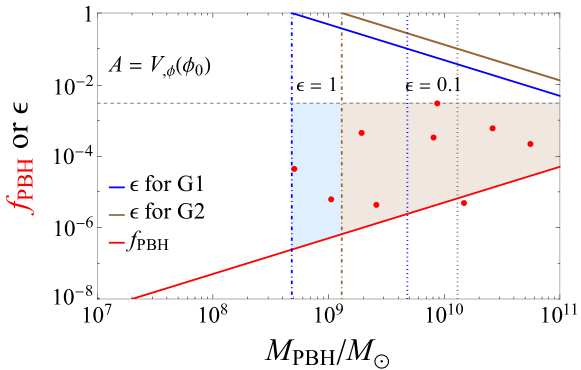
Figure 1: The PBH mass $M_{\rm PBH}$ and abundance $f_{\rm PBH}$ obtained in Case 1 (red dots) around the required ranges for G1 (blue and brown regions) and G2 (brown region) to explain JWST observations with the seed effect. The ordinate of the red part corresponds to the PBH abundance $f_{\rm PBH}$, and that of the blue and brown solid lines correspond to the star formation efficiency $\epsilon$. The ranges of PBH mass and abundance (blue and brown regions) are determined from eqs. (3.6) (black dashed line), (3.8) (red solid line), and (3.9) (blue and brown solid lines). In addition, the dashed-dotted (dotted) lines correspond to $\epsilon=1$ ($\epsilon=0.1$), with blue and brown colors for G1 and G2, respectively. Note that, when the star formation efficiency $\epsilon\lesssim 0.02$, the inflation model can not explain the JWST observations in this case.

Point	$M_{\rm PBH}/M_{\odot}$	$f_{\rm PBH}$	$\phi_{0}/m_{\rm P}$	$\sigma/m_{\rm P}$
${\rm P}_{11}$	$5.1\times 10^{8}$	$4.3\times 10^{-5}$	2.763	0.01550
${\rm P}_{12}$	$1.1\times 10^{9}$	$6.3\times 10^{-6}$	2.770	0.01538
${\rm P}_{13}$	$1.9\times 10^{9}$	$4.4\times 10^{-4}$	2.780	0.01524
${\rm P}_{14}$	$2.6\times 10^{9}$	$4.3\times 10^{-6}$	2.780	0.01522
${\rm P}_{15}$	$8.1\times 10^{9}$	$3.3\times 10^{-4}$	2.796	0.01499
${\rm P}_{16}$	$8.6\times 10^{9}$	$3.0\times 10^{-3}$	2.800	0.01494
${\rm P}_{17}$	$1.5\times 10^{10}$	$4.8\times 10^{-6}$	2.800	0.01491
${\rm P}_{18}$	$2.6\times 10^{10}$	$6.0\times 10^{-4}$	2.810	0.01478
${\rm P}_{19}$	$5.5\times 10^{10}$	$2.1\times 10^{-4}$	2.817	0.01467

Table 1: The PBH masses $M_{\rm PBH}$ and abundances $f_{\rm PBH}$ obtained with the corresponding parameters $\phi_{0}$ and $\sigma$ in Case 1. The parameter $\phi_{0}$ increases $M_{\rm PBH}$, so does $\sigma$ for $f_{\rm PBH}$. It is clear that there exists parameter degeneracy between them.

According to eqs. (3.6), (3.8), and (3.9), we illustrate the expected ranges of PBH mass and abundance for G1 and G2 with different colors in figure 1. The blue region is only valid for G1, but the brown region can explain G1 and G2 together. If $\epsilon\lesssim 0.4$, ${\rm P}_{11}$ and ${\rm P}_{12}$ cannot explain G1, ${\rm P}_{13}$ and ${\rm P}_{14}$ cannot explain G2, while ${\rm P}_{15}$–${\rm P}_{19}$ are valid for both G1 and G2. Furthermore, when $\epsilon\lesssim 0.1$, which is much more reasonable, the inflation model can still explain the JWST observations. It should be noted that ${\rm P}_{17}$ is beyond the blue and brown regions. However, it still has the potential to explain the JWST observations because the solid red line only corresponds to the maximum comoving number densities of G1 and G2 with the overestimated star formation efficiency $\epsilon=1$ [9].

Table 1 indicates that, for a nearly constant PBH abundance $f_{\rm PBH}$, $\phi_{0}$ increases and $\sigma$ decreases with $M_{\rm PBH}$ (${\rm P}_{14}$ and ${\rm P}_{17}$). This is because a larger (smaller) $\phi_{0}$ would enhance (reduce) the power spectrum ${\cal P}_{\cal R}(k)$. To maintain an almost constant ${\cal P}_{\cal R}(k)$, the width $\sigma$ must be much smaller (larger) and leads to a narrower (wider) plateau on $V_{\rm b}$ [i.e., a shorter (longer) USR region]. Also, the parameter $\sigma$ not only increases PBH abundance $f_{\rm PBH}$, but also decreases PBH mass $M_{\rm PBH}$ due to the parameter degeneracy (${\rm P}_{13}$ and ${\rm P}_{14}$, ${\rm P}_{16}$ and ${\rm P}_{17}$).

Moreover, we find that the maximum PBH mass can reach up to $4$–$6\times 10^{10}\,M_{\odot}$ with sufficient abundance for ${\rm P}_{19}$, which covers most of the required mass range. However, it cannot explain the JWST observations if $\epsilon\lesssim 0.02$. The essential reason is that the large-mass PBH is formed in the early stage of the USR inflation, so $M_{{\rm PBH}}$ increases with the parameter $\phi_{0}$. However, when $M_{{\rm PBH}}$ approaches $10^{11}\,M_{\odot}$, a large $\phi_{0}$ will result in a small scalar spectral index $n_{\rm s}<0.957$, inconsistent with the CMB constraint [64]. Therefore, to relieve it on the CMB pivot scale, a third parameter $A_{0}$ is essential, so we next discuss the case with the parameter $A_{0}$.

5.2 Case 2

Now, we consider the more general case, with all the three model parameters $A$, $\phi_{0}$, and $\sigma$ taken into account. In the present case, we set $A=V_{{\rm b},\phi}(\phi_{0})(1+A_{0})$, with a new parameter $A_{0}$ characterizing the deviation of the USR region from a perfect plateau. Since $A_{0}$ plays an opposite role of $\sigma$, the parameter degeneracy between $\phi_{0}$ and $\sigma$ can be largely alleviated.

We again obtain nine favored points (${\rm P}_{21}$–${\rm P}_{29}$) in figure 2, with the relevant model parameters listed in table 2. When $\epsilon\lesssim 0.4$, the PBH mass of ${\rm P}_{21}$ and ${\rm P}_{22}$ are too small to explain G1, so do ${\rm P}_{23}$ and ${\rm P}_{24}$ for G2. Only ${\rm P}_{25}$–${\rm P}_{29}$ are valid for both G1 and G2. When $\epsilon\lesssim 0.1$, there are still four or five points to interpret G1 and G2.

Figure 2: The PBH mass $M_{\rm PBH}$ and abundance $f_{\rm PBH}$ obtained in Case 2 (red dots) around the required range for G1 (blue and brown regions) and G2 (brown region) to explain JWST observations with the seed effect. All the lines and regions have the same meaning as those in figure 1. If the plateau around the USR region is allowed to incline under the influence of the new parameter $A_{0}$, the PBH mass and abundance can cover all the required ranges for interpreting the JWST observations.

Point	$M_{\rm PBH}/M_{\odot}$	$f_{\rm PBH}$	$A_{0}$	$\phi_{0}/m_{\rm P}$	$\sigma/m_{\rm P}$
${\rm P}_{21}$	$5.2\times 10^{8}$	$3.4\times 10^{-4}$	0.01852	2.740	0.01274
${\rm P}_{22}$	$8.0\times 10^{8}$	$6.6\times 10^{-7}$	0.01817	2.745	0.01270
${\rm P}_{23}$	$1.9\times 10^{9}$	$4.6\times 10^{-4}$	0.01825	2.756	0.01255
${\rm P}_{24}$	$2.8\times 10^{9}$	$2.9\times 10^{-3}$	0.01823	2.760	0.01250
${\rm P}_{25}$	$6.7\times 10^{9}$	$1.7\times 10^{-5}$	0.01785	2.770	0.01240
${\rm P}_{26}$	$1.6\times 10^{10}$	$3.4\times 10^{-4}$	0.01751	2.780	0.01230
${\rm P}_{27}$	$4.0\times 10^{10}$	$1.3\times 10^{-3}$	0.01719	2.790	0.01220
${\rm P}_{28}$	$4.0\times 10^{10}$	$2.0\times 10^{-5}$	0.01840	2.800	0.01210
${\rm P}_{29}$	$1.0\times 10^{11}$	$1.9\times 10^{-4}$	0.01675	2.800	0.01211

Table 2: The PBH masses $M_{\rm PBH}$ and abundances $f_{\rm PBH}$ obtained with the corresponding parameters $A_{0}$, $\phi_{0}$, and $\sigma$ in Case 2. The parameter $A_{0}$ has an opposite effect of $\sigma$ in calculating $M_{\rm PBH}$ and $f_{\rm PBH}$, so the parameter degeneracy in Case 1 is relieved to a great extent accordingly.

From table 2, we find that, when $\phi_{0}$ is fixed, the PBH mass $M_{\rm PBH}$ is decreased by $A_{0}$, and the PBH abundance $f_{\rm PBH}$ is enhanced by $\sigma$ (${\rm P}_{28}$ and ${\rm P}_{29}$). Also, when $\phi_{0}$ increases, $A_{0}$ can increase with $M_{\rm PBH}$ unchanged, and $\sigma$ can decrease to reduce $f_{\rm PBH}$ (${\rm P}_{27}$ and ${\rm P}_{28}$). Besides, from the two points ${\rm P}_{13}$ in table 1 and ${\rm P}_{23}$ in table 2, whose PBH masses and abundances are very similar, it is clear to see that the effect of an increasing $A_{0}$ is equivalent to the decrease of both $\phi_{0}$ and $\sigma$, so they are negatively correlated. All these aspects indicate that the parameter degeneracy can be relieved by introducing $A_{0}$. Consequently, the USR inflation model can meet all the required ranges of PBH mass $M_{\rm PBH}\sim 10^{8}$–$10^{11}\,M_{\odot}$ and abundance $f_{\rm PBH}\sim 10^{-5}$–$10^{-3}$, without spoiling the CMB bounds on $n_{\rm s}$ and $r$.

Altogether, in the simple Case 1 with $A=V_{{\rm b},\phi}(\phi_{0})$, the USR inflation model can generate the PBHs to explain the JWST observations as long as $\epsilon\gtrsim 0.02$. Furthermore, in the more general Case 2 with $A=V_{{\rm b},\phi}(\phi_{0})(1+A_{0})$, the USR inflation model can even produce the PBHs that cover the entire required ranges of the PBH mass and abundance for the JWST data.

6 Conclusion

Recently, the JWST observations have attracted wide attention since the massive galaxy candidates with $M_{\ast}\gtrsim 10^{10}M_{\odot}$ at $7.4\lesssim z\lesssim 9.1$ [6] bring a new challenge to the standard $\Lambda$CDM model. Therefore, many mechanisms have been proposed to explain this problem, one of which is the hypothesis that these galaxies are formed through the accretion of supermassive PBHs [23, 24]. Inspired by this insight, we recalculate the PBH mass $M_{\rm PBH}$ and abundance $f_{\rm PBH}$ required to explain the two most extreme high-$z$ objects G1 and G2 [6], and explore a USR inflation model that can generate such supermassive PBHs. Because of the various constraints on $f_{\rm PBH}$ for supermassive PBHs, the possibility of explaining the JWST observations by the Poisson effect of PBHs can be largely ruled out, which is consistent with the point of view in ref. [17]. However, the seed effect can escape these constraints due to its low abundance and nonlinear nature on small scales. This means that such early formation of massive galaxies is possible, if they are seeded by the PBHs that grow in isolation with $10^{8}\,M_{\odot}\lesssim M_{\rm PBH}\lesssim 10^{11}\,M_{\odot}$ and $10^{-7}\lesssim f_{\rm PBH}\lesssim 10^{-3}$.

In this paper, we ideally calculate the ranges of the PBH mass and abundance required for G1 and G2 based on the published version of Ref. [6] and further investigate the possibility of generating these PBHs via the USR inflation. We impose an antisymmetric perturbation $\delta V$ with three model parameters $A$, $\phi_{0}$, and $\sigma$ on the background inflaton potential $V_{\rm b}$. The perturbation naturally leads inflation into the USR phase, during which the power spectrum ${\cal P}_{\cal R}(k)$ of the primordial curvature perturbation can be greatly enhanced on small scales. Thus, it can produce the desired supermassive PBHs, without spoiling the nearly scale-invariant ${\cal P}_{\cal R}(k)$ on the CMB pivot scale.

Two cases are discussed in this work, with $A=V_{{\rm b},\phi}(\phi_{0})$ (Case 1) and $A=V_{{\rm b},\phi}(\phi_{0})(1+A_{0})$ (Case 2), respectively. Both cases can explian G1 and G2 even when $\epsilon\lesssim 0.1$. In Case 1, there can be a perfect plateau on $V_{\rm b}$. The PBH mass $M_{\rm PBH}$ increases with $\phi_{0}$, so does the PBH abundance $f_{\rm PBH}$ with $\sigma$. However, there is still inevitable parameter degeneracy, which provides an upper bound on $M_{\rm PBH}$, making the PBH mass $M_{\rm PBH}$ cannot reach $10^{11}\,M_{\odot}$ yet, though it can cover most of the required range. Nonetheless, in the more general Case 2, with a new parameter $A_{0}$ involved, the plateau on $V_{\rm b}$ is allowed to slightly incline, so the parameter degeneracy is largely relieved. Consequently, the PBH mass $M_{\rm PBH}$ and abundance $f_{\rm PBH}$ can cover their full required ranges to explain the JWST observations.

In summary, with a suitable perturbation on the background inflaton potential, the USR inflation model can produce the PBHs with desired mass and abundance. Albeit such supermassive PBHs cannot contribute a significant fraction of DM, their small abundance is already sufficient to accelerate the formation of massive galaxies at high redshifts via the seed effect, thus deserving further careful consideration. Our work provides a way to reconcile the JWST observations with the standard $\Lambda$CDM model, and is helpful in understanding the JWST data and the early cosmic evolution.

References

- [1] R.P. Naidu, P.A. Oesch, P. van Dokkum, E.J. Nelson, K.A. Suess, G. Brammer et al., Two Remarkably Luminous Galaxy Candidates at – Revealed by JWST, Astrophys. J. Lett. 940 (2022) L14 [arXiv:2207.09434].
- [2] N. Adams, C. Conselice, L. Ferreira, D. Austin, J. Trussler, I. Juodžbalis et al., Discovery and properties of ultra-high redshift galaxies () in the jwst ero smacs 0723 field, Mon. Not. Roy. Astron. Soc. 518 (2023) 4755 [arXiv:2207.11217].
- [3] H. Yan, Z. Ma, C. Ling, C. Cheng and J.-s. Huang, First Batch of – Candidate Objects Revealed by the James Webb Space Telescope Early Release Observations on SMACS 0723-73, Astrophys. J. Lett. 942 (2023) L9 [arXiv:2207.11558].
- [4] H. Atek, M. Shuntov, L.J. Furtak, J. Richard, J.-P. Kneib, G. Mahler et al., Revealing galaxy candidates out to with JWST observations of the lensing cluster SMACS0723, Mon. Not. Roy. Astron. Soc. 519 (2023) 1201 [arXiv:2207.12338].
- [5] C.T. Donnan, D.J. McLeod, J.S. Dunlop, R.J. McLure, A.C. Carnall, R. Begley et al., The evolution of the galaxy UV luminosity function at redshifts – from deep JWST and ground-based near-infrared imaging, Mon. Not. Roy. Astron. Soc. 518 (2023) 6011 [arXiv:2207.12356].
- [6] I. Labbé, P. van Dokkum, E. Nelson, R. Bezanson, K. Suess, J. Leja et al., A population of red candidate massive galaxies Myr after the Big Bang, Nature (2023) [arXiv:2207.12446].
- [7] S.L. Finkelstein, M.B. Bagley, P.A. Haro, M. Dickinson, H.C. Ferguson, J.S. Kartaltepe et al., A Long Time Ago in a Galaxy Far, Far Away: A Candidate Galaxy in Early JWST CEERS Imaging, Astrophys. J. Lett. 940 (2022) L55 [arXiv:2207.12474].
- [8] Y. Harikane, M. Ouchi, M. Oguri, Y. Ono, K. Nakajima, Y. Isobe et al., A Comprehensive Study of Galaxies at – Found in the Early JWST Data: Ultraviolet Luminosity Functions and Cosmic Star Formation History at the Pre-reionization Epoch, Astrophys. J. Suppl. S 265 (2023) 5 [arXiv:2208.01612].
- [9] M. Boylan-Kolchin, Stress Testing CDM with High-redshift Galaxy Candidates, arXiv:2208.01611.
- [10] P.S. Behroozi, R.H. Wechsler and C. Conroy, The Average Star Formation Histories of Galaxies in Dark Matter Halos from –, Astrophys. J. 770 (2013) 57 [arXiv:1207.6105].
- [11] P. Behroozi, R.H. Wechsler, A.P. Hearin and C. Conroy, UNIVERSEMACHINE: The correlation between galaxy growth and dark matter halo assembly from –, Mon. Not. Roy. Astron. Soc. 488 (2019) 3143 [arXiv:1806.07893].
- [12] K. Inayoshi, Y. Harikane, A.K. Inoue, W. Li and L.C. Ho, A Lower Bound of Star Formation Activity in Ultra-high-redshift Galaxies Detected with JWST: Implications for Stellar Populations and Radiation Sources, Astrophys. J. Lett. 938 (2022) L10 [arXiv:2208.06872].
- [13] C.C. Lovell, I. Harrison, Y. Harikane, S. Tacchella and S.M. Wilkins, Extreme value statistics of the halo and stellar mass distributions at high redshift: are JWST results in tension with CDM?, Mon. Not. Roy. Astron. Soc. 518 (2022) 2511 [arXiv:2208.10479].
- [14] N. Menci, M. Castellano, P. Santini, E. Merlin, A. Fontana and F. Shankar, High-redshift Galaxies from Early JWST Observations: Constraints on Dark Energy Models, Astrophys. J. Lett. 938 (2022) L5 [arXiv:2208.11471].
- [15] Y. Gong, B. Yue, Y. Cao and X. Chen, Fuzzy Dark Matter as a Solution to Reconcile the Stellar Mass Density of High- Massive Galaxies and Reionization History, Astrophys. J. 947 (2023) 28 [arXiv:2209.13757].
- [16] M. Biagetti, G. Franciolini and A. Riotto, High-redshift JWST Observations and Primordial Non-Gaussianity, Astrophys. J. 944 (2023) 113 [arXiv:2210.04812].
- [17] G. Hütsi, M. Raidal, J. Urrutia, V. Vaskonen and H. Veermäe, Did JWST observe imprints of axion miniclusters or primordial black holes?, Phys. Rev. D 107 (2023) 043502 [arXiv:2211.02651].
- [18] D. Wang and Y. Liu, JWST high redshift galaxy observations have a strong tension with Planck CMB measurements, arXiv:2301.00347.
- [19] P. Dayal and S.K. Giri, Warm dark matter constraints from the JWST, arXiv:2303.14239.
- [20] A. Ferrara, A. Pallottini and P. Dayal, On the stunning abundance of super-early, luminous galaxies revealed by JWST, Mon. Not. Roy. Astron. Soc. 522 (2023) 3986 [arXiv:2208.00720].
- [21] F. Ziparo, A. Ferrara, L. Sommovigo and M. Kohandel, Blue monsters. Why are JWST super-early, massive galaxies so blue?, Mon. Not. Roy. Astron. Soc. 520 (2023) 2445 [arXiv:2209.06840].
- [22] J. Mirocha and S.R. Furlanetto, Balancing the efficiency and stochasticity of star formation with dust extinction in galaxies observed by JWST, Mon. Not. Roy. Astron. Soc. 519 (2023) 843 [arXiv:2208.12826].
- [23] B. Liu and V. Bromm, Accelerating Early Massive Galaxy Formation with Primordial Black Holes, Astrophys. J. Lett. 937 (2022) L30 [arXiv:2208.13178].
- [24] G.-W. Yuan, L. Lei, Y.-Z. Wang, B. Wang, Y.-Y. Wang, C. Chen et al., Rapidly growing primordial black holes as seeds of the massive high-redshift JWST Galaxies, arXiv:2303.09391.
- [25] Y.B. Zel’dovich and I.D. Novikov, The Hypothesis of Cores Retarded during Expansion and the Hot Cosmological Model, Soviet Astron. AJ (Engl. Transl.), 10 (1967) 602.
- [26] S. Hawking, Gravitationally collapsed objects of very low mass, Mon. Not. Roy. Astron. Soc. 152 (1971) 75.
- [27] S.S. Bavera, G. Franciolini, G. Cusin, A. Riotto, M. Zevin and T. Fragos, Stochastic gravitational-wave background as a tool for investigating multi-channel astrophysical and primordial black-hole mergers, Astron. Astrophys. 660 (2022) A26 [arXiv:2109.05836].
- [28] LIGO Scientific, VIRGO, KAGRA collaboration, Search for Subsolar-Mass Binaries in the First Half of Advanced LIGO’s and Advanced Virgo’s Third Observing Run, Phys. Rev. Lett. 129 (2022) 061104 [arXiv:2109.12197].
- [29] K. Postnov and N. Mitichkin, On the primordial binary black hole mergings in LIGO–Virgo–Kagra data, arXiv:2302.06981.
- [30] S. Matarrese, S. Mollerach and M. Bruni, Second order perturbations of the Einstein-de Sitter universe, Phys. Rev. D 58 (1998) 043504 [astro-ph/9707278].
- [31] T. Papanikolaou, Gravitational waves induced from primordial black hole fluctuations: the effect of an extended mass function, JCAP 10 (2022) 089 [arXiv:2207.11041].
- [32] J.-X. Zhao, X.-H. Liu and N. Li, Primordial black holes and scalar-induced gravitational waves from the perturbations on the inflaton potential in peak theory, Phys. Rev. D 107 (2023) 043515 [arXiv:2302.06886].
- [33] B. Carr and F. Kühnel, Primordial Black Holes as Dark Matter: Recent Developments, Ann. Rev. Nucl. Part. Sci. 70 (2020) 355 [arXiv:2006.02838].
- [34] F. Hoyle and J.V. Narlikar., On the formation of elliptical galaxies, Proc. R. Soc. London A 290 (1966) 177.
- [35] P. Mészáros, Primeval black holes and galaxy formation, Astron. Astrophys. 38 (1975) 5.
- [36] B.J. Carr and J. Silk, Can graininess in the early universe make galaxies?, Astrophys. J. 268 (1983) 1.
- [37] B.J. Carr and M.J. Rees., Can pregalactic objects generate galaxies?, Mon. Not. Roy. Astron. Soc. 206 (1984) 801.
- [38] B. Carr and J. Silk, Primordial Black Holes as Generators of Cosmic Structures, Mon. Not. Roy. Astron. Soc. 478 (2018) 3756 [arXiv:1801.00672].
- [39] B. Carr, K. Kohri, Y. Sendouda and J. Yokoyama, Constraints on primordial black holes, Rept. Prog. Phys. 84 (2021) 116902 [arXiv:2002.12778].
- [40] Y. Inoue and A. Kusenko, New X-ray bound on density of primordial black holes, J. Cosmology Astropart. Phys. 10 (2017) 034 [arXiv:1705.00791].
- [41] B.J. Carr and M. Sakellariadou, Dynamical Constraints on Dark Matter in Compact Objects, Astrophys. J. 516 (1999) 195.
- [42] Planck collaboration, Planck 2018 results. X. Constraints on inflation, Astron. Astrophys. 641 (2020) A10 [arXiv:1807.06211].
- [43] J. Garcia-Bellido and E. Ruiz Morales, Primordial black holes from single field models of inflation, Phys. Dark Univ. 18 (2017) 47 [arXiv:1702.03901].
- [44] C. Germani and T. Prokopec, On primordial black holes from an inflection point, Phys. Dark Univ. 18 (2017) 6 [arXiv:1706.04226].
- [45] G. Ballesteros and M. Taoso, Primordial black hole dark matter from single field inflation, Phys. Rev. D 97 (2018) 023501 [arXiv:1709.05565].
- [46] M. Cicoli, V.A. Diaz and F.G. Pedro, Primordial Black Holes from String Inflation, J. Cosmology Astropart. Phys. 06 (2018) 034 [arXiv:1803.02837].
- [47] J.M. Ezquiaga and J. García-Bellido, Quantum diffusion beyond slow-roll: implications for primordial black-hole production, J. Cosmology Astropart. Phys. 08 (2018) 018 [arXiv:1805.06731].
- [48] J. Liu, Z.-K. Guo and R.-G. Cai, Analytical approximation of the scalar spectrum in the ultraslow-roll inflationary models, Phys. Rev. D 101 (2020) 083535 [arXiv:2003.02075].
- [49] H.V. Ragavendra, P. Saha, L. Sriramkumar and J. Silk, Primordial black holes and secondary gravitational waves from ultraslow roll and punctuated inflation, Phys. Rev. D 103 (2021) 083510 [arXiv:2008.12202].
- [50] A. De and R. Mahbub, Numerically modeling stochastic inflation in slow-roll and beyond, Phys. Rev. D 102 (2020) 123509 [arXiv:2010.12685].
- [51] D.G. Figueroa, S. Raatikainen, S. Rasanen and E. Tomberg, Non-Gaussian Tail of the Curvature Perturbation in Stochastic Ultraslow-Roll Inflation: Implications for Primordial Black Hole Production, Phys. Rev. Lett. 127 (2021) 101302 [arXiv:2012.06551].
- [52] S.-L. Cheng, D.-S. Lee and K.-W. Ng, Power spectrum of primordial perturbations during ultra-slow-roll inflation with back reaction effects, Phys. Lett. B 827 (2022) 136956 [arXiv:2106.09275].
- [53] D.G. Figueroa, S. Raatikainen, S. Rasanen and E. Tomberg, Implications of stochastic effects for primordial black hole production in ultra-slow-roll inflation, J. Cosmology Astropart. Phys. 05 (2022) 027 [arXiv:2111.07437].
- [54] S.S. Mishra, E.J. Copeland and A.M. Green, Primordial black holes and stochastic inflation beyond slow roll: I – noise matrix elements, arXiv:2303.17375.
- [55] O. Özsoy, S. Parameswaran, G. Tasinato and I. Zavala, Mechanisms for Primordial Black Hole Production in String Theory, J. Cosmology Astropart. Phys. 07 (2018) 005 [arXiv:1803.07626].
- [56] S.S. Mishra and V. Sahni, Primordial Black Holes from a tiny bump/dip in the Inflaton potential, J. Cosmol. Astropart. Phys. 04 (2020) 007 [arXiv:1911.00057].
- [57] O. Özsoy and Z. Lalak, Primordial black holes as dark matter and gravitational waves from bumpy axion inflation, J. Cosmology Astropart. Phys. 01 (2021) 040 [arXiv:2008.07549].
- [58] R. Zheng, J. Shi and T. Qiu, On primordial black holes and secondary gravitational waves generated from inflation with solo/multi-bumpy potential, Chin. Phys. C 46 (2022) 045103 [arXiv:2106.04303].
- [59] F. Zhang, J. Lin and Y. Lu, Double-peaked inflation model: Scalar induced gravitational waves and primordial-black-hole suppression from primordial non-Gaussianity, Phys. Rev. D 104 (2021) 063515 [arXiv:2106.10792].
- [60] Y.-C. Liu, Q. Wang, B.-Y. Su and N. Li, Primordial black holes from the perturbations in the inflaton potential, Phys. Dark Univ. 34 (2021) 100905.
- [61] Q. Wang, Y.-C. Liu, B.-Y. Su and N. Li, Primordial black holes from the perturbations in the inflaton potential in peak theory, Phys. Rev. D 104 (2021) 083546 [arXiv:2111.10028].
- [62] M. Sasaki, Large Scale Quantum Fluctuations in the Inflationary Universe, Prog. Theor. Phys. 76 (1986) 1036.
- [63] V.F. Mukhanov, Quantum Theory of Gauge Invariant Cosmological Perturbations, Sov. Phys. JETP 67 (1988) 1297.
- [64] Planck collaboration, Planck 2018 results. VI. Cosmological parameters, Astron. Astrophys. 641 (2020) A6 [arXiv:1807.06209].
- [65] A.M. Green, A.R. Liddle, K.A. Malik and M. Sasaki, A New calculation of the mass fraction of primordial black holes, Phys. Rev. D 70 (2004) 041502 [astro-ph/0403181].
- [66] B.J. Carr and S.W. Hawking, Black holes in the early Universe, Mon. Not. Roy. Astron. Soc. 168 (1974) 399.
- [67] B.J. Carr, The Primordial black hole mass spectrum, Astrophys. J. 201 (1975) 1.
- [68] J.M. Bardeen, J.R. Bond, N. Kaiser and A.S. Szalay, The Statistics of Peaks of Gaussian Random Fields, Astrophys. J. 304 (1986) 15.
- [69] J.C. Niemeyer and K. Jedamzik, Dynamics of primordial black hole formation, Phys. Rev. D 59 (1999) 124013 [astro-ph/9901292].
- [70] I. Musco, J.C. Miller and L. Rezzolla, Computations of primordial black hole formation, Class. Quant. Grav. 22 (2005) 1405 [gr-qc/0412063].
- [71] I. Musco, J.C. Miller and A.G. Polnarev, Primordial black hole formation in the radiative era: Investigation of the critical nature of the collapse, Class. Quant. Grav. 26 (2009) 235001 [arXiv:0811.1452].
- [72] I. Musco and J.C. Miller, Primordial black hole formation in the early universe: critical behaviour and self-similarity, Class. Quant. Grav. 30 (2013) 145009 [arXiv:1201.2379].
- [73] T. Harada, C.-M. Yoo and K. Kohri, Threshold of primordial black hole formation, Phys. Rev. D 88 (2013) 084051 [arXiv:1309.4201].
- [74] T. Nakama, T. Harada, A.G. Polnarev and J. Yokoyama, Identifying the most crucial parameters of the initial curvature profile for primordial black hole formation, J. Cosmology Astropart. Phys. 01 (2014) 037 [arXiv:1310.3007].
- [75] I. Musco, Threshold for primordial black holes: Dependence on the shape of the cosmological perturbations, Phys. Rev. D 100 (2019) 123524 [arXiv:1809.02127].
- [76] A. Escrivà, Simulation of primordial black hole formation using pseudo-spectral methods, Phys. Dark Univ. 27 (2020) 100466 [arXiv:1907.13065].
- [77] A. Escrivà, C. Germani and R.K. Sheth, Universal threshold for primordial black hole formation, Phys. Rev. D 101 (2020) 044022 [arXiv:1907.13311].
- [78] A. Escrivà, C. Germani and R.K. Sheth, Analytical thresholds for black hole formation in general cosmological backgrounds, J. Cosmology Astropart. Phys. 01 (2021) 030 [arXiv:2007.05564].
- [79] I. Musco, V. De Luca, G. Franciolini and A. Riotto, Threshold for primordial black holes. II. A simple analytic prescription, Phys. Rev. D 103 (2021) 063538 [arXiv:2011.03014].
- [80] A.D. Gow, C.T. Byrnes, P.S. Cole and S. Young, The power spectrum on small scales: Robust constraints and comparing PBH methodologies, J. Cosmol. Astropart. Phys. 02 (2021) 002 [arXiv:2008.03289].
- [81] C.-M. Yoo, T. Harada, J. Garriga and K. Kohri, Primordial black hole abundance from random Gaussian curvature perturbations and a local density threshold, Prog. Theor. Exp. Phys. 2018 (2018) 123E01 [arXiv:1805.03946].
- [82] S. Young, C.T. Byrnes and M. Sasaki, Calculating the mass fraction of primordial black holes, J. Cosmol. Astropart. Phys. 07 (2014) 045 [arXiv:1405.7023].
- [83] D. Inman and Y. Ali-Haïmoud, Early structure formation in primordial black hole cosmologies, Phys. Rev. D 100 (2019) 083528 [arXiv:1907.08129].
- [84] B. Liu, S. Zhang and V. Bromm, Effects of stellar-mass primordial black holes on first star formation, Mon. Not. Roy. Astron. Soc. 514 (2022) 2376 [arXiv:2204.06330].
- [85] T. Nakama, B. Carr and J. Silk, Limits on primordial black holes from distortions in cosmic microwave background, Phys. Rev. D 97 (2018) 043525 [arXiv:1710.06945].
- [86] M. Brockamp, H. Baumgardt, S. Britzen and A. Zensus, Unveiling Gargantua: A new search strategy for the most massive central cluster black holes, Astron. Astrophys. 585 (2016) A153 [arXiv:1509.04782].
- [87] R. Murgia, G. Scelfo, M. Viel and A. Raccanelli, Lyman- Forest Constraints on Primordial Black Holes as Dark Matter, Phys. Rev. Lett. 123 (2019) 071102 [arXiv:1903.10509].
- [88] S. Kachru, R. Kallosh, A.D. Linde and S.P. Trivedi, De Sitter vacua in string theory, Phys. Rev. D 68 (2003) 046005 [hep-th/0301240].