The correlations between galaxy properties in different environments of the cosmic web

Abstract

We study the correlations between $(u-r)$ colour, stellar mass, specific star formation rate (sSFR) and metallicity of galaxies in different geometric environments of the cosmic web using a volume limited sample from the SDSS. The geometric environment at the location of each galaxy is determined using the eigenvalues of the tidal tensor in three dimensions. We use the Pearson correlation coefficient (PCC) and the normalized mutual information (NMI) to quantify the correlations between these galaxy properties in sheets, filaments and clusters after matching the stellar mass distributions of the galaxies in these environments. A two-tailed t-test assesses the statistical significance of the observed differences between these relations in different geometric environments. The null hypothesis can be rejected at $>99.99\%$ significance level in most of the cases, suggesting that the scaling relations between the observable galaxy properties are susceptible to the geometric environments of the cosmic web.

1 Introduction

The galaxies are the fundamental units of the large-scale structures in the Universe. A complete understanding of their formation and evolution remains elusive. In the current paradigm, every galaxy is believed to have formed within a dark matter halo. The dark matter halos form from the gravitational collapse of density fluctuations and continue to grow through hierarchical merging. The halos accrete gas from the IGM that radiatively cool and settle down at their centres to form galaxies [1, 2, 3, 4]. The galaxy properties such as mass, morphology, colour, star formation rate and metallicity evolve due to internal processes within galaxies (secular evolution) and interactions with their environment. A host of physical processes such as gas accretion, interaction and merger with other galaxies, star formation, supernovae explosions and AGN feedback shape the galaxy properties, leading to the diversity of galaxies in the present universe.

The external environment play a crucial role in galaxy formation and evolution. Understanding the roles of environment on galaxy properties remains a complex and active area of research. Several studies [5, 6, 7, 8, 9, 10, 11, 12, 13, 14, 15, 16, 17, 18, 19] have been carried out to understand the roles of environment on the galaxy formation and evolution. It is now well known that morphology [6, 20, 21, 22], colour [23, 24, 18, 25], stellar mass [26, 27], star formation rate [28, 29, 30, 31, 32, 15] and many other galaxy properties are strongly correlated with the environment. The environment is generally characterized by the local density in most of these studies. But the large-scale distribution of matter in the universe can not be completely characterized in terms of density. Observations from various redshift surveys [33, 34, 35, 36, 37, 38, 39] reveal that the galaxies are distributed in a complex interconnected network of filaments, sheets and knots surrounded by enormous voids. This network is often referred to as the “cosmic web” [40]. The filaments are usually located at the intersections of sheets and the galaxy clusters are located at the intersections of filaments. The studies with N-body simulations show that matter successively flows from voids to walls, walls to filaments and finally from filaments onto the clusters [41, 42, 43]. It has been suggested by a number of studies with hydrodynamical simulations that more than $80\%$ baryons in the universe reside in filaments in the form of WHIM [46, 47]. The distribution of matter in the cosmic web can affect the gas accretion efficiency of galaxies, influencing their star formation rates [44, 45]. Galaxies that are located near the centers of cosmic filaments and sheets are more likely to receive a steady supply of cold gas from their surroundings, which can fuel star formation and increase the mass of the galaxy. Similarly, the galaxies near the intersections of filaments, tend to have a higher rate of accretion of gas and a higher rate of galaxy interactions, that can trigger intense star formation and alter their internal structures. The galaxies located in the underdense regions of the cosmic web tend to have a more quiescent evolution.

Some studies with hydrodynamical simulations show that the galaxy luminosity function and mass functions depend on the cosmic web environments [60, 61]. The spin of galaxies and their host dark matter halos also show alignment relative to cosmic web filaments [62]. Recently, [63] show that the interacting major pairs at smaller pair separations are more star forming in filaments compared to those hosted in sheets. These together suggest that the geometry of the cosmic web can significantly influence the galaxy properties and their evolution. The observational evidence that the galaxy properties are affected by their large-scale environment is mounting in recent years [24, 31, 64, 65, 66, 67, 68, 69, 70, 71, 72, 73, 74, 75, 76, 77].

The galaxy properties can also be modulated by the mass of its dark matter halo. The intrinsic properties of the halos can influence the galaxy properties through different physical mechanisms such as mass quenching [48, 49, 50, 51] and angular momentum quenching [52]. The properties like mass, shape and spin of the dark matter halos are sensitive to their locations inside the cosmic web [53, 54]. Besides, the clustering of the dark matter halos also depend on their assembly history [55, 56, 57, 58]. [59] show the evidence for halo assembly bias as a function of cosmic web environment using the GAMA survey.

The different galaxy properties such as stellar mass, colour, star formation rate and metallicity are known to be strongly correlated with each other and such correlations may depend on the environment. The blue galaxies are typically lower mass systems with ongoing star formation, while red galaxies are more massive and have mostly ceased star formation. The transition from blue to red galaxies is driven by a process called quenching, in which the SFR decreases and the galaxy becomes redder in colour. Such quenching may be driven by different physical mechanisms such as galaxy harassment [83, 84], starvation [80, 81, 82], strangulation [78, 79], ram pressure stripping [78] and gas outflows through supernovae, AGN or shock-driven winds [85, 86, 87]. A number of internal physical processes such as morphological quenching [88] and bar quenching [89] can also suppress the star formation in galaxies. On the other hand, the star formation activity in galaxies can be significantly enhanced due to interactions [90, 91, 92, 93, 94, 95, 96, 97, 98]. Both galaxy-galaxy interactions and the interactions with the environment are crucial in shaping the correlations between different galaxy properties. The more massive galaxies are generally redder and found in denser environments. The mass and SFR of galaxies are also correlated with their metallicity. The metallicity is a measure of the abundance of elements heavier than Helium in a galaxy. The more massive galaxies have higher metallicities as they are able to retain their heavy elements through repeated rounds of star formation and supernova explosions, which eject heavy elements into the interstellar medium. The low-mass galaxies have shallower gravitational potential wells. This makes it easier for gas to escape during outflows which reduce the overall metallicity of the galaxy. Observations also indicate that galaxies with higher metallicities have lower SFRs [99].

Understanding the observed correlations between different galaxy properties can provide us useful insights on galaxy formation and evolution. The correlations can be qualitatively explained using the equilibrium model of galaxy formation and evolution [100, 101, 102, 103]. It is a simple theoretical model that assumes that the galaxies maintain a steady state, in which the inflow of gas from the IGM is balanced by the outflow of gas due to feedback processes such as supernova explosions and the winds generated by AGN. Galaxies perturbed by interactions, mergers or environment are driven back to their equilibrium and this allows the galaxies to maintain their available gas over time. However, the equilibrium model does not take into account all of the complex processes that contribute to the evolution of galaxies, such as mergers, gravitational interactions, and the influence of large-scale structures. These can be taken into account using N-body simulations or hydrodynamic simulations. These simulations are used to follow the evolution of dark matter and baryonic matter in the universe, and to study the properties of galaxies that form in different environments. Nonetheless, our understanding of the precise nature of the correlations and the physical mechanisms driving them are far from being complete.

It is important to analyze the observational data to understand the correlations between galaxy properties in different environments of the cosmic web. The Sloan Digital Sky Survey (SDSS) [104] is the largest redshift survey carried out till date. It provides high quality spectra and images of millions of galaxies in the universe enabling us to create reliable 3D maps of the galaxy distribution and determine the physical properties of the galaxies with unprecedented accuracy. In the present work, we would like to analyze the SDSS data to study the correlations between a number of galaxy properties in different geometric environments of the cosmic web. We intend to investigate whether these correlations are affected by the geometry of the cosmic web. We plan to identify the galaxies in different environments of the cosmic web based on the signs of the eigenvalues of the tidal tensor [109, 110] at their locations. We will analyze the correlations between stellar mass, colour, star formation rate and metallicity of the galaxies at each type of environment. One can calculate the Pearson correlation coefficient for each pair of galaxy properties in different geometric environments of the cosmic web. The Pearson correlation coefficient measures the linear relationship between two random variables. However some of the relationships between different galaxy properties can be non-linear and non-monotonic. This motivates us to use the mutual information for measuring correlation between galaxy properties. The mutual information is a non-parametric measure for measuring correlations between random variables and it can detect any kind of association, including non-linear and non-monotonic relationships. We will calculate the mutual information for each pair of galaxy properties in different types of geometric environments and test whether they differ in a statistically significant manner. This would help us to quantify the roles of the cosmic web in shaping the correlations between different galaxy properties.

The plan of the paper is as follows. We describe the data in Section 2, explain our methods in Section 3, discuss the results of our analysis in Section 4 and finally present our conclusion in Section 5.

2 Data

We use the publicly available data from the seventeenth data release [105] of the Sloan Digital Sky Survey (SDSS DR17) for the present analysis. DR17 is the fifth and final data release of the fourth phase of the SDSS survey. We use Structured Query Language(SQL) to download the data from the SDSS SkyServer . We select all galaxies within right ascension range $130^{\circ}\leq\alpha\leq 230^{\circ}$ and declination range $0^{\circ}\leq\delta\leq 62^{\circ}$. The SDSS imposed a restriction in the r-band Petrosian apparent magnitude to $\rm m_{r}\leq 17.77$, where only photometric targets brighter than this limit were chosen for follow-up spectroscopy. We construct a volume limited sample by restricting the r-band absolute magnitude to $\mathrm{M_{r}}\,\leq-20$. The resulting volume limited sample radially extends upto $z\leq 0.08$ and contains a total $94986$ galaxies (Figure 1). We obtain the spectroscopic and photometric information of the galaxies from the SpecObjAll and Photoz tables of the SDSS database. We use the observed colour in the present analysis. The colours are not corrected for reddening due to redshift and the internal extinction. The stellar mass, specific star formation rate (sSFR) and metallicity of the galaxies are derived from the table StellarMassFSPSGranWideDust. The sSFR is the star formation rate per unit galaxy stellar mass. The metallicity is the mass fraction of the elements heavier than Helium [106]. These are estimated using the Flexible Stellar Population Synthesis (FSPS) Technique [107]. It models the Spectral Energy Distribution (SED) of galaxies by combining the star formation and metal enrichment histories together with the stellar evolution and dust attenuation. The stellar masses, metallicities and star formation rates are constrained by comparing the observed spectroscopic and/or photometric properties of the galaxies to the stellar population synthesis models. The SDSS spectra are measured through a 3 arcsec aperture which covers only a fraction of the total galaxy. This is usually dealt by fitting the observed spectra with the stellar population synthesis models and then applying a correction based on the the observed colour outside of the fiber [108]. However, the physical properties derived from this approach contain significant systematic uncertainties. [107] show that the information derived solely from the broadband photometry are more robust.

We only consider those galaxies for which the scienceprimary flag is set to 1. This ensures that only the galaxies with best spectroscopic information are included in our analysis. We also compared the redshift distributions of the galaxies in our sample with and without using the scienceprimary flag and find that they are nearly identical.

We finally extract the largest cubic region within our volume limited sample, which has a side length of $183.50\,\mathrm{Mpc}$. It contains a total $24146$ galaxies and has a mean galaxy number density of $\sim 3.933\times 10^{-3}\,\mathrm{Mpc}^{-3}$ (Figure 1). The mean intergalactic separation of the sample is $\approx 6.34\,\rm Mpc$.

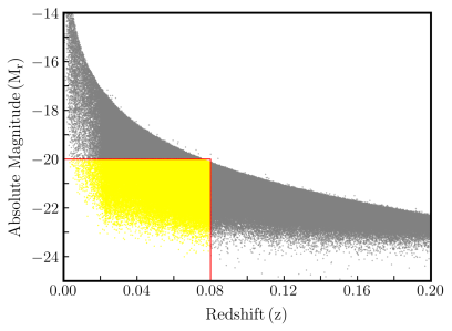
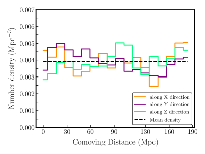
Figure 1: The left panel shows the definition of the volume limited sample in the redshift-absolute magnitude plane. The variations of the comoving number density of galaxies in the extracted cubic region are shown in the right panel. The number density is calculated using slices of thickness $10\,\rm Mpc$.

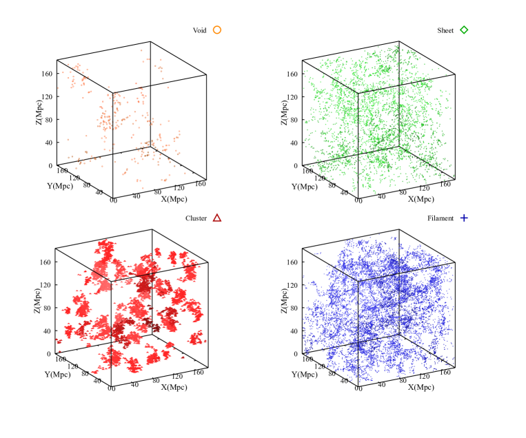
Figure 2: The different panels of this figure show the three-dimensional distributions of galaxies in different cosmic web environments.

3 Method of analysis

3.1 Quantifying the cosmic web

We identify the different morphological components of the cosmic web using the dynamical classification of the cosmic web [109, 110]. This uses the eigenvalues of the three-dimensional tidal tensor to classify the different morphological components. The tidal tensor $T_{\alpha\beta}$ in 3D is defined as the Hessian of the gravitational potential $\Psi$,

$$T_{\alpha\beta}=\frac{\partial^{2}\Psi}{\partial x_{\alpha}\partial x_{\beta}}$$ (3.1)

We first solve the Poisson equation

$$\nabla^{2}\Psi\equiv\delta$$ (3.2)

to obtain the potential. Here $\delta=\frac{\rho-\bar{\rho}}{\bar{\rho}}$ is the density contrast. The galaxy distribution is first converted to a density field by applying the Cloud-in-Cell (CIC) scheme on $(128)^{3}$ grid with a grid spacing of $1.43\,\rm Mpc$. We transform the resulting density field into the Fourier space and multiply it with a Gaussian window function. We use a smoothing length of $7.15\,\rm Mpc$ to achieve a smoothed density distribution. Our galaxy sample does not have a high density. The intergalactic separation in our sample is $\sim 6.34\,\rm Mpc$. The chosen smoothing scale is 5 times the grid spacing, and is close to the intergalactic separation. This choice limits our ability to characterize the environment on scales smaller than the intergalactic separation. In the present work, we are primarily interested in quantifying the large-scale geometric environments in the cosmic web.

We obtain the Fourier transform of the gravitational potential corresponding to the fluctuations in the smoothed density field,

$$\hat{\Psi}=\hat{\mathcal{G}}\hat{\rho}$$ (3.3)

where $\hat{\mathcal{G}}$ is the Fourier counterpart of the Green’s function of the Laplacian operator and $\hat{\rho}$ is the density in Fourier space. We inverse transform the potential back into the real space and calculate the tidal tensor using numerical differentiation of the potential. We classify each galaxy to be part of a void, sheet, filament or cluster based on the signs of the three eigenvalues ($\lambda_{1}$, $\lambda_{2}$, $\lambda_{3}$) of the tidal tensor ( Table 1).

Morphological environment	$\lambda_{1}$	$\lambda_{2}$	$\lambda_{3}$
Void	$<0$	$<0$	$<0$
Sheet	$>0$	$<0$	$<0$
Filament	$>0$	$>0$	$<0$
Cluster	$>0$	$>0$	$>0$

Table 1: This table shows the signs of the three eigen values for each type of morphological environment.

Morphological environment	Number of galaxies present	Number of mass-matched galaxies
Void	$324$	$0$
Sheet	$4435$	$4363$
Filament	$12620$	$4363$
Cluster	$6767$	$4363$

Table 2: This table shows the number of galaxies identified in different morphological environments, using the criteria listed in Table 1.

The number of galaxies identified in different morphological environments are listed in Table 2. We show the three-dimensional distributions of the galaxies identified in different types of geometrical environments in different panels of Figure 2. Our primary aim in this study is to compare the influence of geometric environments on the correlations between different galaxy properties. We do not consider the void galaxies in our analysis due to their lower abundance.

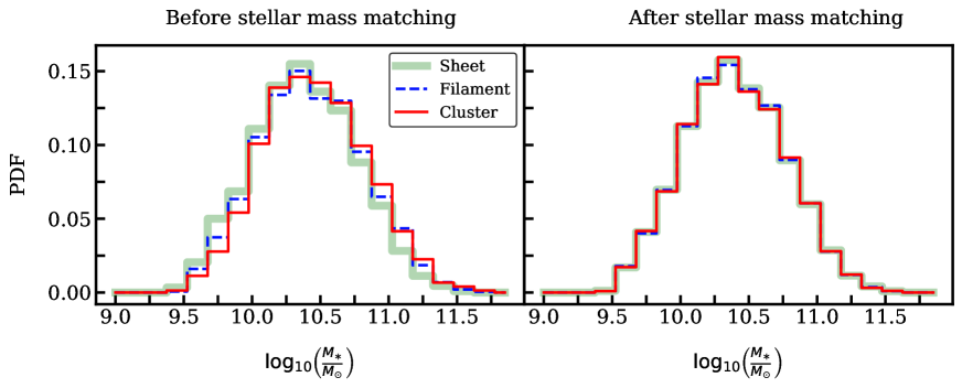
Figure 3: The left panel and right panel of this figure respectively shows the PDF of the stellar mass distributions in different environments before and after matching the stellar mass.

The mass of a galaxy is one of the most important factors influencing the galaxy properties. The strong correlations with the stellar mass can seriously bias our study unless we properly take this into account. The differences in the correlations across various environments may also arise due to the difference in the stellar mass distributions in these environments. It is important to ensure that the results of these analysis are not affected by the link between stellar mass and environment. The sheetlike environments host 4435 galaxies in our dataset. We would like to draw the same number of galaxies from filaments and clusters after matching their mass distributions.This is done in order to have same shot noise contributions in our measurements at each environment. We match the stellar mass (within $0.01$ dex) of equal number of galaxies from the three geometric environments. This provides us with 4363 galaxies in each environment (Table 2). We then use a Kolmogorov-Smirnov (KS) test to compare the PDFs of the stellar mass distribution in different environments. The left and right panels of Figure 3 respectively show the PDFs before and after stellar mass matching. We find that the null hypothesis can be accepted at a very high confidence level ($>99.99\%$) for the stellar mass distributions at each pair of environment. This ensures that the stellar mass distributions of the galaxies in the three different geometric environments are statistically indistinguishable from each other. We carry out our entire analysis using the stellar mass matched samples.

It is worthwhile to mention some limitations of our analysis. The present analysis is carried out in the redshift space, where the “Finger of God” (FOG) effect in the high density groups and clusters may introduce some spurious filaments. Our analysis does not take this effect into account. The volume limited sample used in our analysis does not contain many high density groups/clusters due to the fibre collision effects. Nonetheless, the SDSS spectroscopic sample have completeness issues due to the inherrent limitations from the fibre collisions. The incompleteness issues should be taken into account for a reliable estimation of the environment on small scales. In this work, we are primarily concerned about the large-scale cosmic web environments. These issues may have some impact on our results. However, we do not expect these issues to bias our results in a serious manner.

3.2 Measuring the correlation between different galaxy properties

We use Pearson correlation coefficient and normalized mutual information (NMI) for measuring the correlations between galaxy properties in different geometric environments of the cosmic web.

3.2.1 Pearson correlation coefficient

The Pearson correlation coefficient (PCC) is the simplest measure of linear association between two random variables. It provides the magnitude of the correlation as well as the direction of the relationship.

The PCC for a pair of random variables ($X,Y$) is defined as,

$$r_{XY}=\frac{\sum_{i=1}^{N}(X_{i}-\bar{X})(Y_{i}-\bar{Y})}{\sqrt{\sum_{i=1}^{N}(X_{i}-\bar{X})^{2}\sum_{i=1}^{N}(Y_{i}-\bar{Y})^{2}}}$$ (3.4)

where $\bar{X}=\frac{1}{N}\sum_{i=1}^{N}X_{i}$ and $\bar{Y}=\frac{1}{N}\sum_{i=1}^{N}Y_{i}$ are the average values of $X$ and $Y$ and $N$ is the total number of data points. The PCC ranges from -1 to 1. The values -1 and 1 respectively convey perfect negative correlation and perfect positive correlation between the two random variables.

3.2.2 Normalized mutual information

The relationship between some galaxy properties can be also non-linear and non-monotonic. The mutual information is an information theoretic measure that can detect any kind of association, including non-linear and non-monotonic relationships. Further, it is a non-parametric measure and does not assume a specific distribution for the variables, whereas Pearson correlation assumes a normal distribution. Therefore, the mutual information can be considered to be a more general and robust measure of association compared to the Pearson correlation coefficient.

If $X$ is a discrete random variable which has $n$ possible outcomes {$X_{i}:i=1,\ldots n$} and $P(X_{i})$ is the probability for the $i^{th}$ outcome, then the Shannon entropy corresponding to $X$ is defined as,

$$H(X)=-\sum_{i=1}^{n}P(X_{i})\,\log P(X_{i}).$$ (3.5)

where the base of the logarithm is chosen to be $10$. We consider two discrete random variables $X$ and $Y$ that represent two distinct galaxy properties. The joint entropy of the two variables is determined as,

$$H(X,Y)=-\sum_{i=1}^{n_{1}}\sum_{j=1}^{n_{2}}P(X_{i},Y_{j})\,\log P(X_{i},Y_{j}).$$ (3.6)

where $P(X,Y)$ is the joint probability distribution of $X$ and $Y$. We choose the number of bins to be $n_{1}=n_{2}=20$ for our analysis.

The mutual information (MI) between $X$ and $Y$ is defined as,

$$I(X;Y)=H(X)+H(Y)-H(X,Y)$$ (3.7)

The MI provides a measure of the amount of information one variable conveys about another, regardless of the relationship between them. It does not assume a linear relationship between the two variables. The MI is zero when the two variables are statistically independent.

The NMI [111] is a normalized version of the mutual information. It is defined as,

$$NMI(X;Y)=\frac{I(X;Y)}{\sqrt{H(X)H(Y)}}$$ (3.8)

NMI ranges between 0 and 1, with 1 indicating strongest association between the variables and 0 indicating no association.

The entropy is known to be sensitive to the binning. However this should not be a problem as long as the comparisons are carried out using the same number of bins. We use same number of bins and same number of galaxies for the analysis in each type of geometric environment. This would ensure same level of contributions from shot noise at each environment and allow us to compare the results across the environments in a meaningful way.

We also consider the effects of the binning by repeating our NMI analysis for different number of bins (Appendix A).

4 Results

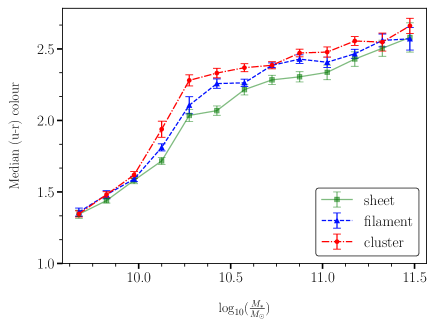
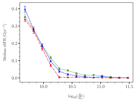
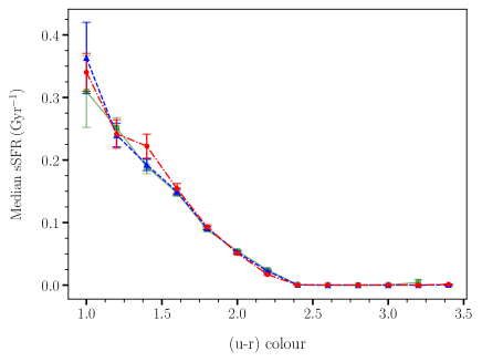
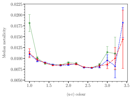
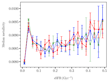
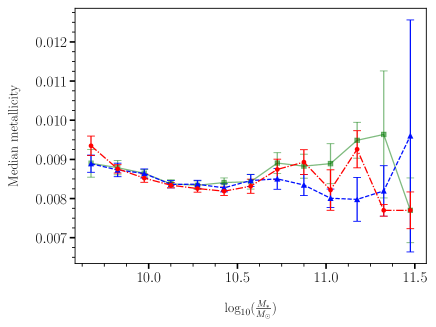
Figure 4: Different panels of this figure show the relation between different pairs of galaxy properties. The x and y axes in each panel represent two different galaxy properties. We do not show the scatter plots for clarity and only show the median values along the y-axes for each values of x. The results for the galaxies in filaments, sheets and clusters are shown together in each panel for comparison. The 1$\sigma$ errors shown on each data point are obtained from 50 bootstrap samples drawn from the original datasets.

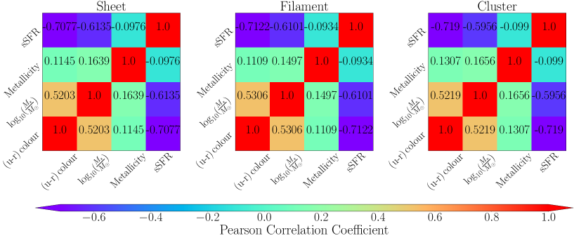
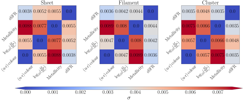
Figure 5: The top three panels of this plot show the Pearson correlation coefficients (PCC) for each pair of the four galaxy properties, $\rm(u-r)\,colour,\,\log_{10}(\frac{M_{\ast}}{M_{\odot}}),\,metallicity,\rm sSFR$ in sheet, filament and cluster, after mass matching. The $1\sigma$ standard deviations corresponding to these measurements are shown in the three bottom panels. The error bars in each case are obtained from 50 jackknife samples drawn from the original datasets.

4.1 Correlations between galaxy properties in filaments, sheets and clusters

We study the correlations between colour, stellar mass, sSFR and metallicity of galaxies in different morphological environments. One can use the scatter plots to investigate the relations between different galaxy properties. However it would be difficult to make a quantitative assessment of the correlations and compare them across different environments. Some of these relations may not be linear and monotonic. We consider a pair of galaxy properties and divide one of them into a number of equal sized bins. We estimate the median value of the other property in each of these bins. We show the binned galaxy property along the x-axes and the median value of the other galaxy property in each bin along the y-axes in different panels of Figure 4. The results for the galaxies in filaments, sheets and clusters are shown together in each panel for comparison.

In the top left panel of Figure 4, we find that the median colour of galaxies in each type of morphological environment increases with the increasing stellar mass. The enhancement of median colour with stellar mass is strongest in the cluster environment followed by the filamentary and sheet-like environments. The differences are more visible above a stellar mass of $10^{10}\,M_{\odot}$. We note that there is a distinct break at $\sim 3\times 10^{10}\,M_{\odot}$ above which the slope of the curves become shallower at each environment. We examine the relationship between the stellar mass and sSFR in the top right panel of Figure 4. We find that the median sSFR decreases with increasing stellar mass. This indicates that star formation plays a more important role in the growth of low-mass galaxies than high-mass galaxies at each environment. A distinct break is also clearly visible at $\sim 3\times 10^{10}\,M_{\odot}$ in every environment. The galaxies above this mass appears to be very low star forming and redder. Thus the colour and sSFR respectively shows a correlation and an anti-correlation with the stellar mass of galaxies. This is consistent with the findings of [112] that the galaxies with stellar mass below $3\times 10^{10}\,M_{\odot}$ are actively star forming whereas those having a larger mass are mostly quenched.

The correlation between colour and stellar mass and an anti-correlation between sSFR and stellar mass suggest that colour and sSFR should be anti-correlated. In the middle left panel of Figure 4, we note that the sSFR and colour of galaxies are anti-correlated in all environments. It may be noted that the galaxies with $(u-r)$ colour above $\sim 2.3$ are very low star forming. These galaxies are expected to be part of the red sequence [113, 114].

We examine the relation between the $(u-r)$ colour and metallicity in the middle right panel of Figure 4. This indicates that the galaxies with redder colour have a higher metallicity in each type of morphological environment. This behaviour is more prominent in the cluster and filament type environments. On the other hand, the bluer galaxies tend to be metal rich in sheet-like environment.

The bottom left panel of Figure 4 show the median metallicity of galaxies as a function of sSFR in each type of morphological environment. This indicates a weak correlation between these two galaxy properties in every environment. We show the median metallicity of galaxies as a function of their stellar mass in different environments in the bottom right panel of Figure 4. The results suggest that the massive galaxies tend to be metal rich in all environments.

Relations	Sheet - Filament		Filament - Cluster		Sheet-Cluster
	$t$ score	$p$ value	$t$ score	$p$ value	$t$ score	$p$ value
colour-stellar mass	$-8.84$	$3.99\times 10^{-14}$	$8.95$	$2.25\times 10^{-14}$	$-1.41$	$1.63\times 10^{-1}$
colour-metallicity	$1.33$	$1.85\times 10^{-1}$	$-11.95$	$7.54\times 10^{-21}$	$-10.41$	$1.58\times 10^{-17}$
colour-sSFR	$6.93$	$4.39\times 10^{-10}$	$10.30$	$2.71\times 10^{-17}$	$15.07$	$2.88\times 10^{-27}$
stellar mass-metallicity	$11.17$	$3.54\times 10^{-19}$	$-11.85$	$1.23\times 10^{-20}$	$-0.39$	$6.98\times 10^{-1}$
stellar mass-sSFR	$-3.29$	$1.39\times 10^{-3}$	$-21.94$	$1.36\times 10^{-39}$	$-23.85$	$1.34\times 10^{-42}$
sSFR-metallicity	$-4.27$	$4.54\times 10^{-5}$	$5.58$	$2.18\times 10^{-7}$	$0.55$	$5.87\times 10^{-1}$

Table 3: This table summarizes the results of a two-tailed t-test after comparing the Pearson correlation coefficients for different pairs of galaxy properties in two different cosmic web environments. The degrees of freedom in this test is $98$.

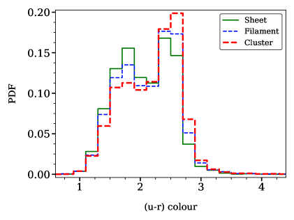
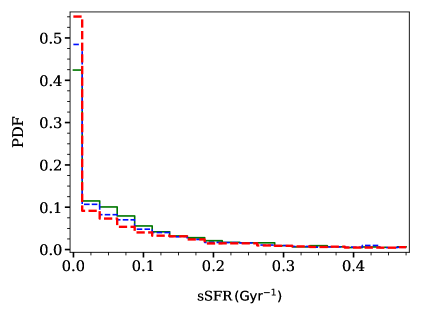
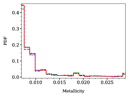
Figure 6: The different panels of this figure show the probability distribution functions (PDF) of $\rm(u-r)$ colour, $\rm sSFR$, and metallicity. The PDFs in sheets, filaments and clusters are shown together in each panel for comparison.

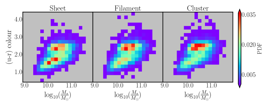
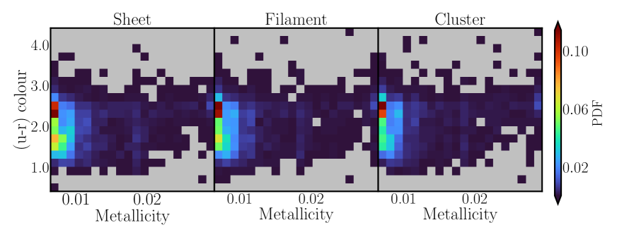
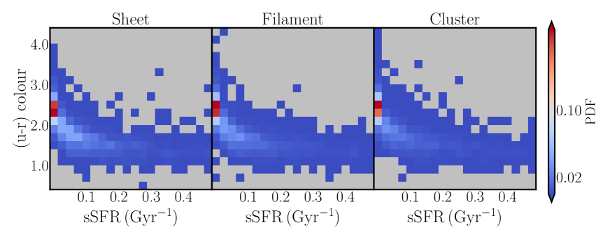
Figure 7: The top, middle and bottom panels of this figure respectively show the joint probability distribution of $(u-r)$ colour with stellar mass, metallicity and sSFR in different geometric environments.

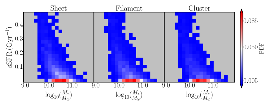
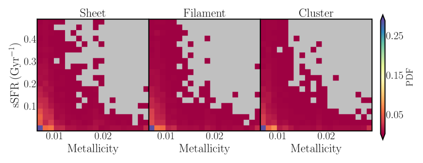
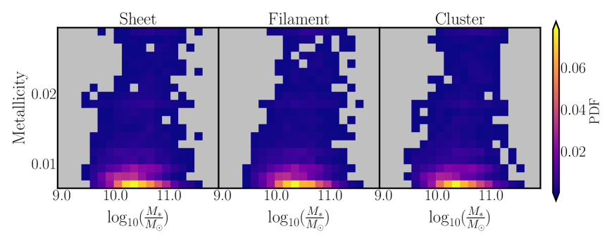
Figure 8: Same as Figure 7 but for different pairs of galaxy properties.

4.2 Measuring the correlations with the Pearson correlation coefficient

In subsection 4.1, we use Figure 4 to infer the relations between different galaxy properties in a qualitative manner. One can quantify the magnitudes and directions of these correlations by measuring the PCC between each pair of galaxy properties in different morphological environments.

We show the PCCs for different pairs of galaxy properties in each type of cosmic web environments in the upper panels of Figure 5. The $1\sigma$ errors in each of these measurements are shown in the bottom panels of the same figure. The $1\sigma$ errors are obtained from 50 jackknife samples drawn from the original datasets. In the top three panels, we find that the sSFR shows anti-correlation with each of the other three galaxy properties in all types of morphological environments. Out of these three pairs, the sSFR-stellar mass and sSFR-(u-r) colour are strongly anti-correlated whereas the sSFR-metallicity is weakly anti-correlated. Metallicity shows relatively stronger correlations with (u-r) colour and stellar mass. The stellar mass is strongly correlated with the (u-r) colour in all environments which partly explains the observed positive correlations for the metallicity-stellar mass and metallicity-(u-r) colour relations. The PCC for each pair of galaxy properties in each environment are significantly larger compared to the $1\sigma$ errors in the respective measurements. So the measured correlations and anti-correlations between different galaxy properties are statistically significant. The PCC corresponding to each pair of galaxy properties differ by a small amount across the different environments. Interestingly, the $1\sigma$ errors for the correlation coefficients are also very small.

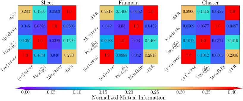
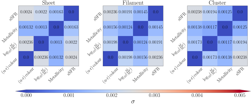
Figure 9: Same as Figure 5 but for NMI. We choose 20 bins for this NMI analysis.

We use a two-tailed t-test to determine if the observed PCC for various pairs of galaxy properties are significantly different in filaments, sheets and clusters. We compare the relations for separate geometric environments. The t-score and p-value corresponding to each relation are obtained in different pair of geometric environments and listed in Table 3. We find a strong evidence against the null hypothesis for most of the relations in different cosmic web environments. However, the null hypothesis can not be rejected for the colour-stellar mass, stellar mass-metallicity and sSFR-metallicity relations in sheet and cluster. The same is true for the colour-metallicity relation in sheet and filament. We note that the majority of the relations are strongly sensitive to the geometric environments of the cosmic web. It may be noted that these relations are somewhat non-linear and non-monotonic (Figure 4). The PCC may not be ideally suited for measuring the correlations between these galaxy properties. We address this limitation of PCC by employing NMI for our analysis in the next subsection.

Relations	Sheet - Filament		Filament - Cluster		Sheet-Cluster
	$t$ score	$p$ value	$t$ score	$p$ value	$t$ score	$p$ value
colour-stellar mass	$13.83$	$9.26\times 10^{-25}$	$-6.42$	$4.79\times 10^{-9}$	$8.79$	$5.09\times 10^{-14}$
colour-metallicity	$13.46$	$5.16\times 10^{-24}$	$-29.94$	$4.13\times 10^{-51}$	$-18.24$	$2.90\times 10^{-33}$
colour-sSFR	$1.79$	$7.68\times 10^{-2}$	$-19.69$	$7.67\times 10^{-36}$	$-17.72$	$2.55\times 10^{-32}$
stellar mass-metallicity	$11.26$	$2.29\times 10^{-19}$	$-30.79$	$3.48\times 10^{-52}$	$-18.40$	$1.45\times 10^{-33}$
stellar mass-sSFR	$-2.78$	$6.54\times 10^{-3}$	$-1.93$	$5.66\times 10^{-2}$	$-4.55$	$1.53\times 10^{-5}$
sSFR-metallicity	$17.08$	$3.82\times 10^{-31}$	$-13.58$	$2.90\times 10^{-24}$	$5.50$	$3.08\times 10^{-7}$

Table 4: This table shows the $t$ scores and $p$ values calculated using Student’s t-test after comparing the normalized mutual information between different pairs of galaxy properties in two separate cosmic web environments. We have used a two-tailed t-test for our analysis. The degrees of freedom in this test is $98$. 20 bins are used for this analysis.

4.3 Quantifying the correlations using the normalized mutual information

In subsection 4.2, we use the PCC to measure the correlations and anti-correlations between different galaxy properties in various cosmic web environments. The PCC fails to capture any non-linear and non-monotonic behaviour in these relationships. We see that the relationship between the different galaxy properties are not entirely linear (subsection 4.1). So we also employ NMI to study the correlations between these galaxy properties. This requires us to calculate the probability distribution functions (PDF) for each galaxy property as well as the 2D probability distribution functions corresponding to each pair of galaxy properties.

We show the PDFs of (u-r) colour, sSFR and metallicity in the three panels of Figure 6. In the top left panel of Figure 6, we find that the clusters host a larger fraction of the red galaxies and a lower fraction of the blue galaxies. We see a similar trend in filaments. Interestingly, the sheets host a comparable fraction of the red and the blue galaxies. The top right panel of Figure 6 shows the PDFs of sSFR in sheets, filaments and clusters. The PDFs show that the galaxies hosted in the sheets and filaments are relatively high star forming than those located in the clusters. Similar differences can be noticed in the bottom panel of Figure 6 which shows the PDFs of metallicity in different morphological environments.

We show the joint probability distributions of different pairs of galaxy properties in Figure 7 and Figure 8. A closer look at these plots suggests that there are similarities as well as differences in these PDFs across the different cosmic environments. We can see a distinct galaxy population with a very low sSFR and metallicity that lies within $10<\log_{10}(\frac{M_{\ast}}{M_{\odot}})<11$ and $2.25<(u-r)<2.75$ in these plots. This population represents the quiescent galaxies that are undergoing a transition due to either secular evolution or environmental influences. A higher concentration of such galaxies in clusters indicates that they provide a favourable environment for quenching. It is clear that the transitional population is present across all types of environments in the cosmic web.

We use these PDFs and the joint PDFs to calculate the NMI between galaxy properties in different cosmic web environments. The NMI between different galaxy properties in sheets, filaments and clusters are shown in the top three panels of Figure 9. We find a non-zero NMI for each pair of galaxy properties in all the cosmic web environments. The 1$\sigma$ errors in each of these measurements are also shown in the bottom three panels of the same figure. The errors are estimated from 50 jackknife samples drawn from the original datasets.

In the top three panels of Figure 9, we find that the sSFR shows a relatively stronger correlation with colour and stellar mass and a weaker correlation with metallicity. The correlation of metallicity with colour and stellar mass are also relatively weaker in all three environments. The correlation between colour and stellar mass is reasonably stronger in all environments. It may be noted that NMI does not provide the direction for any of these relationships. However it is a better measure of correlations in presence of non-linearity and non-Gaussianity. We use a two-tailed t-test in order to asses the statistical significance of the differences in the NMI in different geometric environments. We list the t-scores and p-values corresponding to each relation for each pair of geometric environments in Table 4. The p-values suggest that the null hypothesis can be rejected for most of the relations in different pairs of geometric environments. We note that there are weaker evidences against the null hypothesis for the stellar mass-sSFR relation in filament and cluster. Also, the null hypothesis can not be rejected for the colour-sSFR relation in sheet and filament.

We use the same number of galaxies (4363) and the same number of bins (20) across all the geometric environments in our NMI analysis. The specific choice of bins may have an influence on our results. We consider the effects of binning by repeating the NMI analysis for two other choices of the number of bins (15 and 25). The corresponding results are shown in Figure 10 and Figure 11 respectively. The values of the t-scores and p-values for the two cases are listed in Table 5 and Table 6. We find that the null hypothesis can be rejected for most of the relations irrespective of our choice of the number of bins. Our conclusions remain unchanged, and hence are robust against the choice of the number of bins.

The analysis with PCC and NMI agree on discarding the null hypothesis for most of the relations. There are a few differences too. The null hypothesis for the colour-sSFR relation in sheet-filament and the stellar mass-sSFR relation in filament-cluster can be rejected if PCC is used instead of NMI. On the other hand, the NMI analysis allows us to reject the null hypothesis for which PCC provides weak evidences (e.g. colour-stellar mass, stellar mass-metllicity relations in Sheet-Cluster). Given the non-linear nature of the relationships, the NMI should be preferred over the PCC in breaking any such ambiguities. Finally, the results of our analysis clearly indicate that the correlations between different galaxy properties are strongly sensitive to the geometric environments of the cosmic web.

5 Conclusions

We analyze the correlations between $(u-r)$ colour, stellar mass, sSFR and metallicity in different geometric environments of the cosmic web. The geometric environments of the galaxies are identified using the eigenvalues of the 3D tidal tensor. We use Pearson correlation coefficient (PCC) and the normalized mutual information to study the correlations. The PCC is a well known measure of correlation that assumes Gaussianity in the distributions of the variables and linearity in their relationships. However, this may not hold true for each galaxy property and every relationship. The NMI does not make any assumption regarding the distribution of the variables and the nature of relationship between them. It is positive by definition and hence can not capture the direction in a relation unlike the PCC. Its primary advantage is that it can efficiently capture the correlations even when the relationships are non-linear and non-monotonic. We use the NMI as a complimentary measure of correlation between the galaxy properties. We compare the observed PCC and NMI between the galaxy properties across the different geometric environments. Using a two-tailed t-test, we investigate if the mean PCC and NMI in sheet, filament and cluster are significantly different. Both the PCC and the NMI allow us to reject the null hypothesis for most of the relations in different environments. The null hypothesis could not be rejected in only two instances out of eighteen while using NMI and four cases out of eighteen while using PCC. We believe that NMI is a better choice for our study due to the non-linear nature of the relationships. Our results suggest that most of the scaling relations are strongly sensitive to the cosmic web environment.

The relationship between the galaxy properties and the environment is a complex issue. Galaxies follow different evolutionary pathways. Both the local environment and the geometry of the cosmic web may have significant influences on the evolution of galaxy properties. Any such dependence may also modulate the scaling relations in different environments. Studies with the hydrodynamical simulations suggest that the cosmic web dependence of the galaxy properties is primarily driven by the variation of halo mass functions with environment [60, 61]. Some earlier studies with the SDSS data find that the galaxy properties have a weak dependence on the cosmic web environments [115, 116, 117]. On the other hand, several other works demonstrate the roles of the cosmic web in deciding the galaxy properties [68, 73, 24, 31, 71, 72]. The galaxy properties are also known to be influenced by the tidal environments [65, 69]. The spin and shape of the dark matter halos are known to have alignment with their host environments [122, 123]. Some recent studies with simulations and observations show that the cosmic filaments have spin on unprecedented scales [124, 125]. Using the SDSS data, [118] show that galaxy properties exhibit clear dependence on the connectivity of the cosmic web at fixed stellar mass. Such dependence on the connectivity of the cosmic web suggests that it has crucial roles in providing the main source of fuel for galaxy growth. An analysis of the IllustrisTNG simulation [119] by [120] find significant dependence of galaxy properties on the cosmic web environment. They show that the cosmic web structures efficiently channel cold gas into most galaxies leading to such dependence. Our results are consistent with these findings. These together suggest that the large-scale geometric environments have important roles in the galaxy evolution.

Nevertheless, the interpretation of our results may be affected by a number of issues related to the density and structural variety of the structures. The various cosmic web environments represent the regions of different overdensity. The clusters are generally denser than the filaments and the filaments are relatively denser than the sheets. The local density and the geometric environments are expected to have combined influences on the galaxy properties and their correlations. It is difficult to separate these influences in our study. We tried to carry out an analysis by restricting the local density within a fixed range for each environment. However, this provides us with a very small number of galaxies at each environment. There are other subtle issues that are not addressed in the present work. For example, the filaments around the massive clusters may have different density and morphology than filaments around the low-mass clusters. The filaments may have different visual morphology such as long, short, straight, curved, warped etc [121]. The environmental influences on galaxies in massive clusters and low mass clusters are also expected to be different. It would be interesting to study these relationships in structures of different mass and visual morphology. These may be considered as some caveats in our analysis. We plan to study these issues in greater detail in a future study using the Illustris simulations [119]. Further, the sensitivity of the correlations to the geometric environment may depend on the details of the galaxy formation models as well as the background cosmological models. It would be interesting to investigate these issues using simulations.

Finally, we conclude from our study that the correlations between different galaxy properties are susceptible to the geometric environments of the cosmic web.

Appendix A Appendix

We repeat our NMI analysis for 15 bins and 25 bins. The respective results are shown in Figure 10 and Figure 11 respectively. We list the t-scores and p-values for the two cases in Table 5 and Table 6.

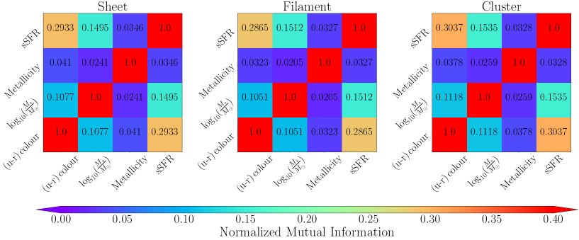
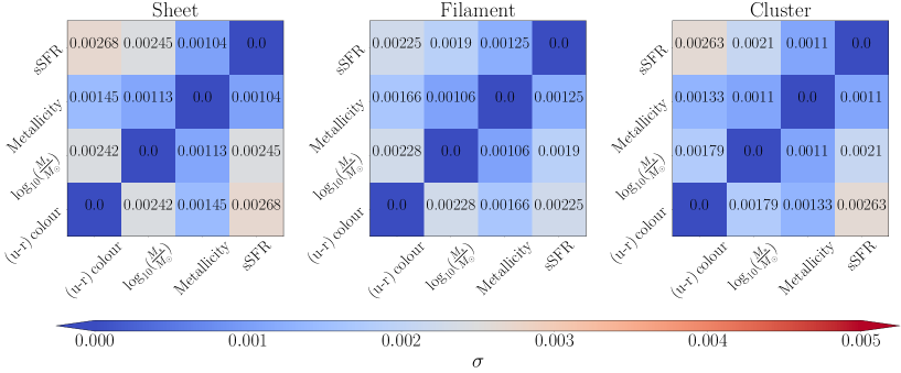
Figure 10: Same as Figure 9 but for 15 bins.

Relations	Sheet - Filament		Filament - Cluster		Sheet-Cluster
	$t$ score	$p$ value	$t$ score	$p$ value	$t$ score	$p$ value
colour-stellar mass	$4.78$	$6.08\times 10^{-6}$	$-15.38$	$7.02\times 10^{-28}$	$-9.51$	$1.41\times 10^{-15}$
colour-metallicity	$28.06$	$1.24\times 10^{-48}$	$-19.89$	$3.54\times 10^{-36}$	$9.94$	$1.62\times 10^{-16}$
colour-sSFR	$14.99$	$4.17\times 10^{-27}$	$-37.07$	$1.82\times 10^{-59}$	$-20.22$	$9.55\times 10^{-37}$
stellar mass-metallicity	$16.14$	$2.33\times 10^{-29}$	$-24.97$	$2.88\times 10^{-44}$	$-8.27$	$6.59\times 10^{-13}$
stellar mass-sSFR	$-4.85$	$4.61\times 10^{-6}$	$-4.57$	$1.44\times 10^{-5}$	$-8.66$	$9.59\times 10^{-14}$
sSFR-metallicity	$8.50$	$2.12\times 10^{-13}$	$-0.75$	$4.58\times 10^{-1}$	$8.32$	$5.20\times 10^{-13}$

Table 5: Same as Table 4 but for 15 bins.

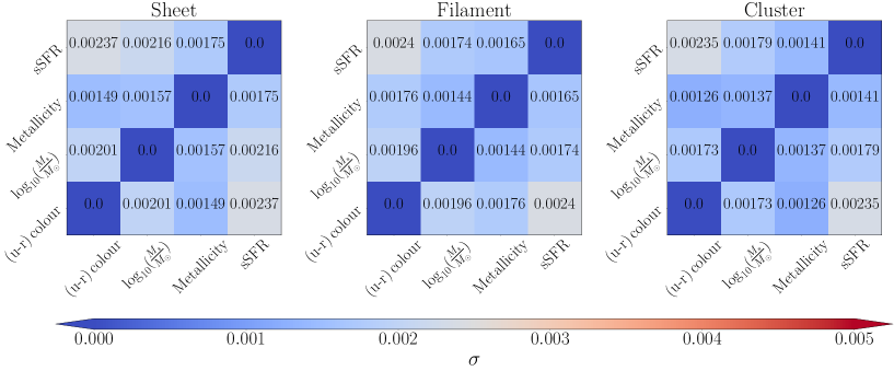
Figure 11: Same as Figure 9 but for 25 bins.

Relations	Sheet - Filament		Filament - Cluster		Sheet-Cluster
	$t$ score	$p$ value	$t$ score	$p$ value	$t$ score	$p$ value
colour-stellar mass	$10.01$	$1.13\times 10^{-16}$	$-15.58$	$2.87\times 10^{-28}$	$-4.77$	$6.49\times 10^{-6}$
colour-metallicity	$16.66$	$2.41\times 10^{-30}$	$-6.62$	$1.94\times 10^{-9}$	$12.33$	$1.22\times 10^{-21}$
colour-sSFR	$3.59$	$5.19\times 10^{-4}$	$-23.08$	$2.06\times 10^{-41}$	$-19.59$	$1.17\times 10^{-35}$
stellar mass-metallicity	$-1.57$	$1.21\times 10^{-1}$	$-13.51$	$4.21\times 10^{-24}$	$-14.51$	$3.74\times 10^{-26}$
stellar mass-sSFR	$-0.85$	$3.97\times 10^{-1}$	$-8.32$	$5.37\times 10^{-13}$	$-8.24$	$7.97\times 10^{-13}$
sSFR-metallicity	$10.06$	$9.09\times 10^{-17}$	$12.25$	$1.75\times 10^{-21}$	$22.59$	$1.25\times 10^{-40}$

Table 6: Same as Table 4 but for 25 bins.

References

- [1] M. J. Rees & J. P. Ostriker, MNRAS, 179, 541 (1977)
- [2] J. Silk, ApJ, 211, 638 (1977)
- [3] S. D. M. White & M. J. Rees, MNRAS, 183, 341 (1978)
- [4] S. M. Fall & G. Efstathiou, MNRAS, 193, 189 (1980)
- [5] M. Davis & M.J. Geller, ApJ, 208, 13 (1976)
- [6] A. Dressler, ApJ, 236, 351 (1980)
- [7] H. R. Butcher & Jr. A. Oemler, Nature, 310, 31 (1984)
- [8] L. Guzzo, M.A. Strauss, K.B. Fisher, R. Giovanelli & M.P. Haynes, ApJ, 489, 37 (1997)
- [9] I. Zehavi, et al., ApJ, 571, 172 (2002)
- [10] T. Goto, C. Yamauchi, Y. Fujita, S. Okamura, M. Seikiguchi, I. Smail, M. Bernardi & P.L. Gomez, MNRAS, 346, 601 (2003)
- [11] D. W. Hogg, et al., ApJ Letters, 585, L5 (2003)
- [12] M. R. Blanton, et al., ApJ, 594, 186 (2003)
- [13] J. Einasto, G. Hütsi, M. Einasto, E. Saar, D. L. Tucker, V. Müller, P. Heinämäki & S. S. Allam, A&A, 405, 425 (2003)
- [14] M. L. Balogh, I. Smail, R. G. Bower, et al., ApJ, 566, 123 (2002)
- [15] G. Kauffmann, S. D. M. White, T. M. Heckman, et al., MNRAS, 353, 713 (2004)
- [16] U. Abbas & R. K. Sheth, MNRAS, 372, 1749 (2006)
- [17] M. Mouhcine, I. K. Baldry & S. P. Bamford, MNRAS, 382, 801 (2007)
- [18] S. P. Bamford, R. C. Nichol, I. K. Baldry, et al, MNRAS, 393, 1324 (2009)
- [19] Y. Koyama, I. Smail, J. Kurk, et al., MNRAS, 434, 423 (2013)
- [20] C.N.A. Willmer, L.N. da Costa & P.S. Pellegrini, AJ, 115, 869 (1998)
- [21] I. Zehavi, et al., ApJ, 630, 1 (2005)
- [22] C. Park, et al., ApJ, 633, 11 (2005)
- [23] I. K. Baldry, M. L. Balogh, R. G. Bower, et al., MNRAS, 373, 469 (2006)
- [24] B. Pandey & S. Bharadwaj, MNRAS, 372, 827 (2006)
- [25] K. Kreckel, E. Platen, M. A. Aragón-Calvo, et al., AJ, 144, 16 (2012)
- [26] G. Chabrier, Publications of the Astronomical Society of the Pacific, 115, 763 (2003)
- [27] Y.-j. Peng, S. J. Lilly,, K, Kovač, et al., ApJ, 721, 193 (2010)
- [28] A. Toomre & J. Toomre, ApJ, 178, 623 (1972)
- [29] I. Lewis, M. Balogh, R. De Propris, et al., MNRAS, 334, 673 (2002)
- [30] P. L. Gómez, R. C. Nichol, C. J. Miller, et al., ApJ, 584, 210 (2003)
- [31] B. Pandey & S. Bharadwaj, MNRAS, 387, 767 (2008)
- [32] S. C. Porter, S. Raychaudhury, K. A. Pimbblet & M. J. Drinkwater, MNRAS, 388, 1152 (2008)
- [33] S. A. Gregory, L. A. Thompson, ApJ, 222, 784 (1978)
- [34] M. Joeveer, J. Einasto, IAUS, 79, 241 (1978)
- [35] J. Einasto, M. Joeveer, E. Saar, MNRAS, 193, 353 (1980)
- [36] I. B. Zeldovich, S. F. Shandarin, PAZh, 8, 131 (1982)
- [37] J. Einasto, A. A. Klypin, E. Saar, S. F. Shandarin, MNRAS, 206, 529 (1984)
- [38] S. Bharadwaj, V. Sahni, B. S. Sathyaprakash, S. F. Shandarin, C. Yess, ApJ, 528, 21 (2000)
- [39] B. Pandey, S. Bharadwaj, MNRAS, 357, 1068 (2005)
- [40] J. R. Bond, L. Kofman, & D. Pogosyan, Nature, 380, 603 (1996)
- [41] M. A. Aragón-Calvo, E. Platen, R. van de Weygaert, A. S. Szalay, ApJ, 723, 364 (2010)
- [42] M. Cautun, R. van de Weygaert, B. J. T. Jones, C. S. Frenk, 2014, MNRAS, 441, 2923 (2014)
- [43] N. S. Ramachandra, S. F. Shandarin, MNRAS, 452, 1643 (2015)
- [44] N. Cornuault, M. Lehnert, F. Boulanger, P. Guillard, A&A, 610, A75 (2018)
- [45] W. Zhu, F. Zhang, L.-L. Feng, ApJ, 924, 132 (2022)
- [46] T. Tuominen, J. Nevalainen, E. Tempel, T. Kuutma, N. Wijers, J. Schaye, P. Heinämäki, et al., A&A, 646, A156 (2021)
- [47] D. Galarraga-Espinosa, N. Aghanim, M. Langer, H. Tanimura, A&A, 649, A117 (2021)
- [48] Y. Birnboim, & A. Dekel, MNRAS, 345, 349 (2003)
- [49] A. Dekel, & Y. Birnboim, MNRAS, 368, 2 (2006)
- [50] D. Kereš , N. Katz, D. H. Weinberg, & R. Davé , MNRAS, 363, 2 (2005)
- [51] J. M. Gabor, R. Davé , K. Finlator, & B. D. Oppenheimer, MNRAS, 407, 749 (2010)
- [52] Y.-. jie Peng ., A. Renzini, MNRAS, 491, L51 (2020)
- [53] O. Hahn, C. Porciani, C. M. Carollo & A. Dekel, MNRAS, 375, 489 (2007)
- [54] J. Lee, V. Springel, U.-L. Pen, G. Lemson, MNRAS, 389, 1266 (2008)
- [55] D. J. Croton, L. Gao, S. D. M. White, MNRAS, 374, 1303 (2007)
- [56] L. Gao, S. D. M. White, MNRAS, 377, L5 (2007)
- [57] M. Musso, C. Cadiou, C. Pichon, S. Codis, K. Kraljic, Y. Dubois, MNRAS, 476, 4877 (2018)
- [58] M. Vakili, C. Hahn, ApJ, 872, 115 (2019)
- [59] R. Tojeiro, E. Eardley, J. A. Peacock, P. Norberg, M. Alpaslan, S. P. Driver, B. Henriques, et al., MNRAS, 470, 3720 (2017)
- [60] G. Metuki, N. I. Libeskind, Y. Hoffman, R. A. Crain, T. Theuns, MNRAS, 446, 1458 (2015)
- [61] W. Xu, Q. Guo, H. Zheng, L. Gao, C. Lacey, Q. Gu, S. Liao, et al., MNRAS, 498, 1839 (2020)
- [62] P. Ganeshaiah Veena, M. Cautun, E. Tempel, R. van de Weygaert, C. S. Frenk, MNRAS, 487, 1607 (2019)
- [63] A. Das, B. Pandey, S. Sarkar, RAA, 23, 025016 (2023)
- [64] I. Trujillo, C. Carretero & S. G. Patiri, ApJ Letters, 640, L111 (2006)
- [65] J. Lee & P. Erdogdu, ApJ, 671, 1248 (2007)
- [66] D. J. Paz, F. Stasyszyn & N. D. Padilla, MNRAS, 389, 1127 (2008)
- [67] B. J. T. Jones, R. van de Weygaert & M. A. Aragón-Calvo, MNRAS, 408, 897 (2010)
- [68] J. M. Scudder, S. L. Ellison, & J. T. Mendel, MNRAS, 423, 2690 (2012)
- [69] E. Tempel & N. I. Libeskind, ApJ Letters, 775, L42 (2013)
- [70] E. Tempel, R. S. Stoica & E, Saar, MNRAS, 428, 1827 (2013)
- [71] B. Darvish, D. Sobral, B. Mobasher, et al., ApJ, 796, 51 (2014)
- [72] M. E. Filho, J. Sánchez Almeida, C. Muñoz-Tuñón, et al., ApJ, 802, 82 (2015)
- [73] H. E. Luparello, M. Lares, D. Paz, et al., MNRAS, 448, 1483 (2015)
- [74] B. Pandey & S. Sarkar, MNRAS, 467, L6 (2017)
- [75] J. Lee, ApJ, 867, 36 (2018)
- [76] Y.-C. Chen, S. Ho, J. Blazek, S. He, R. Mandelbaum, P. Melchior, S. Singh, MNRAS, 485, 2492 (2019)
- [77] B. Pandey & S. Sarkar, MNRAS, 498, 6069 (2020)
- [78] J. E. Gunn, & J. R. Gott, ApJ, 176, 1 (1972)
- [79] M. L. Balogh, J. F. Navarro, & S. L. Morris, ApJ, 540, 113 (2000)
- [80] R. B. Larson, B. M. Tinsley, & C. N. Caldwell, ApJ, 237, 692 (1980)
- [81] R. S. Somerville, & J. R. Primack, MNRAS, 310, 1087 (1999)
- [82] D. Kawata, & J. S. Mulchaey, ApJL, 672, L103 (2008)
- [83] B. Moore, N. Katz, G. Lake, A. Dressler, & A. Oemler, Nature, 379, 613 (1996)
- [84] B. Moore, G. Lake, & N. Katz, ApJ, 495, 139 (1998)
- [85] T. J. Cox, J. Primack, P. Jonsson, & R. S. Somerville, ApJL, 607, L87 (2004)
- [86] N. Murray, E. Quataert, & T. A. Thompson, ApJ, 618, 569 (2005)
- [87] V. Springel, T. Di Matteo, & L. Hernquist, MNRAS, 361, 776 (2005)
- [88] M. Martig, F. Bournaud, R. Teyssier, & A. Dekel, ApJ, 707, 250 (2009)
- [89] K. L. Masters, M. Mosleh, A. K. Romer, R. C. Nichol, S. P. Bamford, K. Schawinski, C. J. Lintott, et al., MNRAS, 405, 783 (2010)
- [90] E. J. Barton, M. J. Geller, S. J. Kenyon, ApJ, 530, 660 (2000)
- [91] D. G. Lambas, P. B. Tissera, M. S. Alonso, G. Coldwell, MNRAS, 346, 1189 (2008)
- [92] M. S. Alonso, P. B. Tissera, G. Coldwell, D. G. Lambas, MNRAS, 352, 1081 (2004)
- [93] B. Nikolic, H. Cullen, P. Alexander, P., MNRAS, 355, 874 (2004)
- [94] S. L. Ellison, D. R. Patton, L. Simard, A. W. McConnachie, I. K. Baldry, J. T. Mendel, MNRAS, 407, 1514 (2010)
- [95] D. F. Woods, M. J. Geller, M. J. Kurtz, E. Westra, D. G. Fabricant, I. Dell’Antonio, AJ, 139, 1857 (2010)
- [96] D. R. Patton, S. L. Ellison, L. Simard, A. W. McConnachie, J. T. Mendel, MNRAS, 412, 591 (2011)
- [97] G. Violino, S. L. Ellison, M. Sargent, K. E. K. Coppin, J. M. Scudder, T. J. Mendel, A. Saintonge, MNRAS, 476, 2591 (2018)
- [98] M. D. Thorp, S. L. Ellison, H.-A. Pan, L. Lin, D. R. Patton, A. F. L. Bluck, D. Walters, et al., MNRAS, 516, 1462 (2022)
- [99] F. Mannucci, G. Cresci, R. Maiolino, A. Marconi, A. Gnerucci, MNRAS, 408, 2115 (2010)
- [100] A. Dekel, R. Sari, D. Coverino, ApJ, 703, 785 (2009)
- [101] R. Davé, K. Finlator, B. D. Oppenheimer, MNRAS, 416, 1354 (2011)
- [102] R. Davé, K. Finlator, B. D. Oppenheimer, MNRAS, 421, 98 (2012)
- [103] S. J. Lilly, C. M. Carollo, A. Pipino, A. Renzini, Y. Peng, ApJ, 772, 119L (2013)
- [104] C. Stoughton, R. H. Lupton, M. Bernardi, M. R. Blanton, S. Burles, F. J. Castander, A. J. Connolly, et al., AJ, 123, 485 (2002)
- [105] Abdurro’uf, K. Accetta, C. Aerts, V. Silva Aguirre, R. Ahumada, N. Ajgaonkar, N. Filiz Ak, et al., ApJS, 259, 35 (2022)
- [106] M. Asplund, N. Grevesse, A. J. Sauval, P. Scott, ARA&A, 47, 481 (2009)
- [107] C. Conroy, J. E. Gunn, & M. White, ApJ, 699, 486 (2009)
- [108] J. Brinchmann, S. Charlot, S. D. M. White, C. Tremonti, G. Kauffmann, T. Heckman, J. Brinkmann J., MNRAS, 351, 1151 (2004)
- [109] O. Hahn, C. Porciani, C. M. Carollo & A. Dekel, MNRAS, 381, 41 (2007)
- [110] J. E. Forero–Romero, Y. Hoffman, S. Gottlöber, A. Klypin, G. Yepes, MNRAS, 396, 1815 (2009)
- [111] A. Strehl & J. Ghosh, Journal of Machine Learning Research, 3, 583 (2002)
- [112] G. Kauffmann, T. M. Heckmann, S. D. M. White, S. Charlot, C. Tremonti, et al., MNRAS, 341, 54 (2003)
- [113] I. Strateva, Ž. Ivezić, G. R. Knapp, V. K. Narayanan, M. A. Strauss, J. E. Gunn, R. H. Lupton, et al., AJ, 122, 1861 (2001)
- [114] B. Pandey, MNRAS, 499, L31 (2020)
- [115] A. Paranjape, O. Hahn, R. K. Sheth, MNRAS, 476, 5442 (2018)
- [116] S. Alam, Y. Zu, J. A. Peacock, R. Mandelbaum, MNRAS, 483, 4501 (2019)
- [117] T. Kuutma, A. Poudel, M. Einasto, P. Heinämäki, H. Lietzen, A. Tamm, E. Tempel, A&A, 639, A71 (2020)
- [118] K. Kraljic, C. Pichon, S. Codis, C. Laigle, R. Davé, Y. Dubois, H. S. Hwang, et al., MNRAS, 491, 4294 (2020)
- [119] M. Vogelsberger, S. Genel, V. Springel, P. Torrey, D. Sijacki, D. Xu, G. Snyder, et al., Nature, 509, 177 (2014)
- [120] F. Hasan, J. N. Burchett, A. Abeyta, D. Hellinger, N. Mandelker, J. R. Primack, S. M. Faber, et al.,ApJ,950, 114 (2023)
- [121] K. A. Pimbblet, M. J. Drinkwater, M. C. Hawkrigg, MNRAS, 354, L61 (2004)
- [122] P. Wang, Q. Guo, X. Kang, N. I. Libeskind, ApJ, 866, 138 (2018)
- [123] Veena P. Ganeshaiah, M. Cautun, R. van de Weygaert, E. Tempel, B. J. T. Jones, S. Rieder, C. S. Frenk, MNRAS, 481, 414 (2018)
- [124] Q. Xia, M. C. Neyrinck, Y.-C. Cai, M. A. Aragón-Calvo, MNRAS, 506, 1059 (2021)
- [125] P. Wang, N. I. Libeskind, E. Tempel, X. Kang, Q. Guo, Nature Astronomy, 5, 839 (2021)