SMUG Planner: A Safe Multi-Goal Planner for Mobile Robots in Challenging Environments

Abstract

Robotic exploration or monitoring missions require mobile robots to autonomously and safely navigate between multiple target locations in potentially challenging environments. Currently, this type of multi-goal mission often relies on humans designing a set of actions for the robot to follow in the form of a path or waypoints. In this work, we consider the multi-goal problem of visiting a set of pre-defined targets, each of which could be visited from multiple potential locations. To increase autonomy in these missions, we propose a safe multi-goal (SMUG) planner that generates an optimal motion path to visit those targets. To increase safety and efficiency, we propose a hierarchical state validity checking scheme, which leverages robot-specific traversability learned in simulation. We use LazyPRM* with an informed sampler to accelerate collision-free path generation. Our iterative dynamic programming algorithm enables the planner to generate a path visiting more than ten targets within seconds. Moreover, the proposed hierarchical state validity checking scheme reduces the planning time by $30\%$ compared to pure volumetric collision checking and increases safety by avoiding high-risk regions. We deploy the SMUG planner on the quadruped robot ANYmal and show its capability to guide the robot in multi-goal missions fully autonomously on rough terrain.

I INTRODUCTION

Multi-goal missions are commonly seen in exploration, inspection, and monitoring scenarios. In those missions, a robot needs to visit numerous targets of interest for detailed investigation, for example to deploy instruments, collect samples, or read measurements from gauges. However, in current missions, the autonomy of the robot to navigate and plan is limited and relies on human operators [arches, esa, hvdc].

Space exploration is a common application of such multi-goal missions. One example is the geological mission I of the ARCHES analog demonstration mission [arches]. In this mission, a flying system and a rover map the environment and detect multiple targets of interest. A second rover collects samples and returns them to the landing system one at a time according to scientists’ prioritization. A planner that generates a global path visiting all identified targets according to the map provided by other robots could increase the autonomy of the robot team. Another space exploration example is the launched by the and the  [esa] that simulates a lunar prospecting mission, in which multiple targets need to be mapped and characterized. Several teams used a multi-robot strategy to map the environment and find the targets before starting a close-up investigation of the targets. However, none of the teams used a multi-goal planner: They either operated via waypoints provided by an operator or used heuristics to always visit the next closest target.

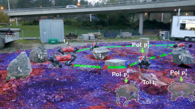
Figure 1: The ANYmal quadruped robot autonomously performs a multi-goal mission of visiting six stones (Targets of Interest (ToIs):$t_{i}$) at one of the corresponding Pose of Interest (PoI): $p_{i}^{j}$ following the global path colored in green. The traversability map is overlaid on the real scene. The red regions are untraversable whereas the blue regions are traversable. The PoIs $p_{1}^{1},p_{1}^{2},p_{1}^{3}$ for the ToI $t_{1}$ are indicated by the green arrows. $p_{1}^{2}$ is selected, whereas the other two not selected PoIs are gray.

Apart from exploration missions, multi-goal navigation is also relevant for industrial inspection and monitoring tasks. An example is the ARGOS (Autonomous Robot for Gas and Oil Sites) Challenge [argos] initiated by the company Total and ANR, in which the robots are required to navigate over a decommissioned gas dehydration skid to perform inspection tasks, such as reading sensor dials and valve positions, at various targets. Gehring et al. [hvdc] provide a solution to the industrial inspection of an offshore HVDC platform with the ANYmal quadruped robot. After the environment is mapped using the onboard sensors, the operator records the desired target location, at which detailed visual or thermal inspection needs to be done, and defines the via-point for the robot.

No planner exists that allows for fully autonomous multi-goal mission conduction. This results in such missions mostly relying on human operators, causing delays, sub-optimal decision-making, and limiting efficiency.

In this paper, we present SMUG planner, a multi-goal planner to plan a safe path to visit a set of targets at the poses in their vicinity for detailed investigation. We refer to the targets as and the valid poses to visit them as , as illustrated in Fig. 1. More precisely, we present a planner to visit one per , which we refer to as multi-goal mission in this paper. This is the with collision-free path planning. The large number of collision-free paths involved in the problem makes it impossible to simply deploy an off-the-shelf solver, such as GLNS [glns], which would require computing all collision-free paths and results in infeasible computational cost. How to efficiently ensure the safety and the optimality of the global path makes this an especially challenging problem.

SMUG planner implements a two-stage planning schema: At first the optimal visit sequence of the s using a  [tsp] solver is determined. Secondly, the optimal to visit each is determined using in an iterative fashion, which we refer to as . We use LazyPRM* [rrt*] with an informed sampler to efficiently generate the optimal collision-free paths. To guarantee safety, we propose a hierarchical obstacle avoidance strategy using a robot-specific traversability estimation module [lvn]. This design allows for replanning during the mission and onboard deployment. SMUG planner can therefore guarantee autonomy in communication-denied environments, which are common in many exploration and monitoring scenarios.

Our contributions consist of the following:

• A multi-goal path planner for mobile robots solving the GTSP with collision-free paths that can generate a safe path to visit more than ten targets in seconds.

• A novel obstacle avoidance scheme that reduces the planning time by 30% compared to the pure volumetric collision checking and avoids high-risk regions.

• Hardware deployment on the ANYmal legged robot in a multi-goal mission on rough terrain. To the best of our knowledge, this is the first time a global planner is deployed to a real-world GTSP with collision-free path planning on a mobile robot.

II RELATED WORK

Our work builds upon prior work developed in the context of sampling-based path planning and methods for solving the and its variants modeling multi-goal problems. Given our objective of real-world deployment, we specifically review existing global planners deployed on mobile robots.

Sampling-Based Path Planning

One family of popular path planning methods is sampling-based path planners [rapid, nbv, gbp, art], which allows for a continuous state space instead of discretization as in grid-based methods.  [prm], and its optimal version PRM* [rrt*] build a probabilistic roadmap for the environment and effectively reuse the information collected across different queries, making these planners suitable for planning across multiple start-goal pairs in the same environment. Because the collision-checking of nodes and edges is costly and efficiency is important to our planner, LazyPRM* [lazyprm*] is well-suited, since it only checks edge validity if it may construct the optimal path, which reduces the planning time. Gammel et al. [informed] proposed to restrict the sampling space based on the cost of the best path found so far, thus accelerating path improvement. Our method builds upon LazyPRM* with an informed sampler to achieve efficient path planning in multi-goal missions.

Multi-Goal Sequencing Problem

is the problem of finding the optimal sequence visiting a set of targets. A instance considers each target as a single point. Its two variants,  [gtsp] and  [tspn], consider the targets as sets of points and continuous neighborhoods respectively. This approach is more accurate in many real-world scenarios, where a point often only needs to be approached instead of visited exactly. Exact algorithms proposed to solve include using Branch and Cut [ant], Lagrangian relaxation [lagrangian] or transforming to an equivalent instance [transform]. Other works solving and based on heuristics such as the ant-colony optimization [antcolony], genetic algorithm [rkga, hrkga] and Lin-Kernighan heuristic [lk] or formulate the problem as  [minlp]. However, these works ignore the computationally expensive collision-free path planning for a mobile robot navigating in complex environments. Alatartsev et al. [onoptimizing] divide the into two subproblems: Given the visiting point of each target, find the optimal visiting sequence. And given the visiting sequence, find the optimal visiting points. These subproblems are solved iteratively. Although the obstacle avoidance necessary in a real-world scenario is ignored, the strategy of splitting the into two subproblems is insightful, and we adopt it in our method. Gentilini [hrkga] focuses on combinatorial optimization with while assuming all path costs are known a priori. However, the author provides two cases in simulation that consider obstacle avoidance, which is achieved by planning the required collision-free path for each chromosome in the genetic algorithm, making it expensive and thus unsuitable for our problem that requires the fast online generation of safe paths.

The variants of and addressing collision-free path planning are called  [mtp] and  [mtpgr] respectively. Gao et al. [automatic] divide the into two subproblems as in [onoptimizing]. However, instead of iterating between them, they first solve for the optimal sequence once. Then, the path between any two points is initially assumed to be the straight line, and refined by alternating iteratively using the  [rba] to find the visiting point and planning the needed path accordingly. Thus, collision-free paths are only planned if they may construct the optimal global path, largely reducing the number of paths to plan. However, the is prone to locally optimal path cost, since it adjusts the visiting point solely based on the two neighboring paths. Moreover, the authors only illustrate their method on a 2D grid map and lack real-world demonstration.

Instead of solving , we model the multi-goal problem as an by assuming the s to be discrete sets of s rather than a continuous neighborhood, because one may want to deploy an instrument to the s, which requires a certain angle of attack or impose other constraints, resulting in disconnected valid s. However, the most general choice is to model each as a set of disconnected neighborhoods, which results in  [gtspn]. Our assumption of each being a discrete set simplifies the problem, while still allowing for multiple valid proposals.

Planners for Mobile Robots

Multiple existing planners for mobile robots have been successfully deployed in the real world [gbp, gbp2, tare, nbv]. Although they are not designed for the multi-goal mission, we use previously proven concepts and design patterns.

Several works adopted a bifurcated global and local planning structure [gbp, gbp2, tare], where the local planner has detailed information in the vicinity of the robot, handles obstacle avoidance, and is guided by a global planner with coarser paths. Following this structure, we generate the entire traversing path and use it to guide a local planner that refines the path locally at a higher frequency.

A discrete volumetric map is often used to represent the environment [gbp, gbp2, nbv], which can be obtained by Voxblox [voxblox]. In [gbp] [nbv], and [gbp2], the authors consider the volumetric collision with the environment, however, not accounting for terrain traversability, which is crucial for the feasibility and safety of the path followed by a local planner. Therefore, we propose to leverage an in simulation-trained legged robot-specific traversability module [lvn], within the global planner, to evaluate the robot-specific terrain traversability.

III PROBLEM STATEMENT

We aim to solve the problem of finding the safe global path that visits every in multi-goal missions. We formulate the problem as an . The robot can visit a at multiple s in a neighborhood of it. In this work, we limit the problem to visiting one per .

Let $\mathcal{C}$ be the state space representing the environment and $\mathcal{C}_{collision}$ the set consisting of the states in $\mathcal{C}$ that result in a collision between the robot and environment. The collision-free space is therefore $\mathcal{C}_{free}=\mathcal{C}\setminus\mathcal{C}_{collision}$. A path is denoted as a discrete representation through a set of waypoints, i.e. $W(w_{0},w_{n})=\left\{w_{0},w_{1},w_{2},…,w_{n}\right\}$ with $w_{i}\in\mathcal{C}$. $W$ represents the path starting at state $w_{0}$, traversing through $w_{1}$, $w_{2}$ …, and ending at $w_{n}$. The cost of a path segment $\{w_{i},w_{i+1}\}$ is given by a positive definite function $c(\cdot,\cdot):\mathcal{C}\times\mathcal{C}\mapsto\mathbb{R}_{\geq 0}$. The total cost of the path $W$ is the sum of the cost of all its path segments, i.e.:

$$Cost(W(w_{0},w_{n}))=\sum_{i=0}^{n-1}{c(w_{i},w_{i+1})}.$$ (1)

The input and output of the problem are summarized as:

Input:

• Robot start and end pose $s\in\mathcal{C}_{free}$.

• A set of poses $\mathcal{T}=\{t_{i}|t_{i}\in\mathcal{C},i\in\{1,\cdots,n\}\}$ with $t_{i}\in\mathcal{C}$.

• For each $t_{i}$, a set of $n_{i}$ $\mathcal{P}_{i}=\{p_{i}^{j}|p_{i}^{j}\in\mathcal{C}_{free},j\in\{1,\cdots,m_{i}\}\}$.

Output: A collision-free path $W(w_{0},w_{n})=\left\{w_{0},...,w_{n}\right\}$ with minimum cost visiting every $t_{i}\in\mathcal{T}$ at a $p_{i}^{j}\in\mathcal{P}_{i}$, starting at $s$ and ending at the same state:

$$\min_{W} Cost(W)$$ (2)

s.t. $$p_{i}^{j}\in W,\forall{t_{i}\in\mathcal{T}},\exists{p_{i}^{j}\in\mathcal{P}_{i}},$$

$$w_{0}=w_{n}=s,$$

$$w_{i}\in\mathcal{C}_{free},\forall w_{i}\in W$$

The constraint $w_{n}=s$ can be relaxed but is used here to facilitate the notation. In this work, the state space $\mathcal{C}$ is chosen to be $SE(2)$, suitable for ground robots. A state $s$is thus expressed by its 2D coordinates $x_{s},y_{s}$ and yaw $\psi_{s}$ as

$$s=\begin{bmatrix}x_{s},y_{s},\psi_{s}\end{bmatrix}^{\top}.$$ (3)

For the cost function $c(\cdot,\cdot):\mathcal{C}\times\mathcal{C}\mapsto\mathbb{R}_{\geq 0}$, we use the  [ompl] default distance function in $SE(2)$:

$$c(s_{1},s_{2})=w_{t}\left\|\begin{bmatrix}x_{s_{1}}\\ y_{s_{1}}\end{bmatrix}-\begin{bmatrix}x_{s_{2}}\\ y_{s_{2}}\end{bmatrix}\right\|_{2}^{2}+w_{r}d(\psi_{s_{1}},\psi_{s_{2}}),$$ (4)

where $w_{t},w_{r}\in\mathbb{R}^{+}$ are the weights for the translational and the rotational cost, respectively, and $d(\cdot,\cdot):[-\pi,\pi]^{2}\mapsto[0,\pi]$ is defined as

$$d(\psi_{1},\psi_{2})=\min{(|\psi_{1}-\psi_{2}|,2\pi-|\psi_{1}-\psi_{2}|)},$$ (5)

to compute the difference between two angles.

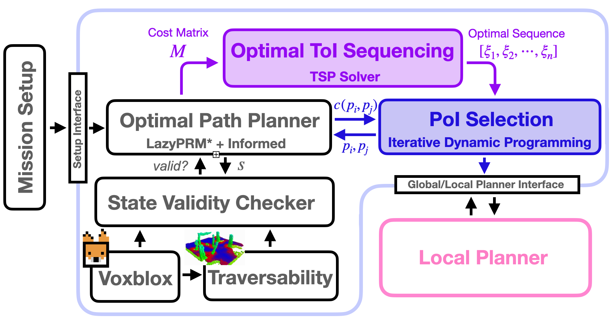
Figure 2: System overview of the SMUG planner illustrating the information flow from accepting the mission to interacting with a low-level local planner. First, the optimal Target of Interest (ToI) sequence is computed (purple, Section IV-C). Second, the best Pose of Interest (PoI) is selected for each ToI (blue, Section IV-D). Our sampling-based optimal path planner (Section IV-A) is used in both steps to generate optimal collision-free paths. State validity is determined via geometric traversability checking in a volumetric map provided prior to the planning (Section IV-B).

IV METHOD

Solving the directly is challenging due to the large number of possibly collision-free paths. Therefore, we adopt a two-step method similar to [automatic]. In the first step, we determine the optimal sequence that visits every by simplifying the problem to a . This simplification is valid, assuming that the s are close to the respective s. In the second step, we select the at each to minimize the total path cost. Fig. 2 shows an overview of our system. The system consists of the following modules:

1. An optimal path planner generating the optimal path connecting two states (Section IV-A);

2. A state validity checker using the and the traversability map provided by Voxblox [voxblox] and a traversability module [lvn], respectively, prior to the planning(Section IV-B);

3. A solver computing the optimal visiting sequence of the s given a cost matrix containing the path cost between each pair of s (Section IV-C);

4. An module selecting the optimal for each that minimizes the total path cost (Section IV-D);

5. A local planner [art] generating a finer path locally that follows the received global path.

IV-A Optimal Path Planning

We use LazyPRM* [lazyprm*] with an informed sampler to generate the optimal collision-free paths between two states.

The sampler initially samples uniformly in $SE(2)$. After an initial path is found, it restricts the sample space based on the cost function and the current path cost to accelerate path optimization. Based on the informed sampler for the $L_{2}$ cost [informed], we implement an informed sampler for the cost function $c(\cdot,\cdot)$ (Eq. 4).

Assume the path to find starts at state $s_{1}$ and ends at state $s_{2}$, and an initial path with cost $c_{0}$ is already found. The new sample $s_{new}$ are sampled in the ellipsoid

$$\mathcal{E}\!=\!\left\{\!\begin{bmatrix}x\\ y\end{bmatrix}\!\Bigg{|}\!\left\|\begin{bmatrix}x\\ y\end{bmatrix}\!-\!\begin{bmatrix}x_{s_{1}}\\ y_{s_{1}}\end{bmatrix}\right\|^{2}_{2}\!+\!\left\|\begin{bmatrix}x\\ y\end{bmatrix}\!-\!\begin{bmatrix}x_{s_{2}}\\ y_{s_{2}}\end{bmatrix}\right\|^{2}_{2}\!<\!c_{0}\!-\!c_{r}\!\right\},$$ (6)

where $c_{r}=d(\psi_{s_{1}},\psi_{s_{2}})$. Any sample $s$ outside this ellipsoid cannot improve the cost due to the following equation

$$c(s_{1},s)+c(s,s_{2})$$ (7)

$$= \left\|\begin{bmatrix}x_{s_{1}}\\ y_{s_{1}}\end{bmatrix}-\begin{bmatrix}x_{s}\\ y_{s}\end{bmatrix}\right\|^{2}_{2}+\left\|\begin{bmatrix}x_{s}\\ y_{s}\end{bmatrix}-\begin{bmatrix}x_{s_{2}}\\ y_{s_{2}}\end{bmatrix}\right\|^{2}_{2}$$

$$+d(\psi_{s_{1}},\psi_{s})+d(\psi_{s},\psi_{s_{2}})$$

$$\geq \left\|\begin{bmatrix}x_{s_{1}}\\ y_{s_{1}}\end{bmatrix}-\begin{bmatrix}x_{s}\\ y_{s}\end{bmatrix}\right\|^{2}_{2}+\left\|\begin{bmatrix}x_{s}\\ y_{s}\end{bmatrix}-\begin{bmatrix}x_{s_{2}}\\ y_{s_{2}}\end{bmatrix}\right\|^{2}_{2}+d(\psi_{s_{1}},\psi_{s_{2}})$$

$$\geq c_{0}-c_{r}+c_{r}=c_{0}.$$

Then, the yaw angle $\psi_{s_{new}}$ is sampled uniformly in $[-\pi,\pi]$. This procedure is summarized below:

if path found then

       $c_{r}\leftarrow d(\psi_{s_{1}},\psi_{s_{2}})$;

       $c_{0}\leftarrow\textit{best cost}$;

       $x,y\leftarrow\textit{SampleInformedL2}(s_{1},s_{2},c_{0}-c_{r})$;

      

else

       $x\leftarrow\textit{SampleUniform}(x_{min},x_{max})$;

       $y\leftarrow\textit{SampleUniform}(y_{min},y_{max})$;

      

end if

$\psi\leftarrow\textit{SampleUniform}(-\pi,\pi)$;

$s_{new}\leftarrow[x,y,\psi]^{\top}$;

return $s_{new}$

Algorithm 1 Sample$()$

The sampled states are passed to a state validity checker to avoid states in collision with the environment.

IV-B State Validity Checker

We use a hierarchical obstacle avoidance scheme to ensure the feasibility and safety of the generated path efficiently. We adopt a robot-specific traversability module learned in simulation to accept the clearly safe states and discard clearly unsafe ones. Only states with unclear safety are checked for collision in an iterative volumetric fashion.

IV-B1 Traversability Filtering

We use a learned traversability map output by a convolutional neural network [lvn], which takes the occupancy map as its input. The network assigns for each voxel a traversability estimate ranging from $0$ to $1$ based on the success rate of traversing through this voxel in simulation as illustrated in Fig. 3(a). We use this module to reduce the amount of iterative collision checking. The traversability is divided into three levels by setting two thresholds $t_{low}$ and $t_{high}$, satisfying $0\leq t_{low}\leq t_{high}\leq 1$. We obtained the traversability of a continuous state $s$ defined in Eq. 3 by querying the corresponding traversability voxel. States with traversability less than $t_{low}$ are directly invalidated, while those with traversability higher than $t_{high}$ are validated. Only states with traversability between $t_{low}$ and $t_{high}$ are checked for collisions. This avoids checking collisions for obviously valid states, for instance, the states in the middle of a wide open space, as well as definitely invalid states that lie within an obstacle.

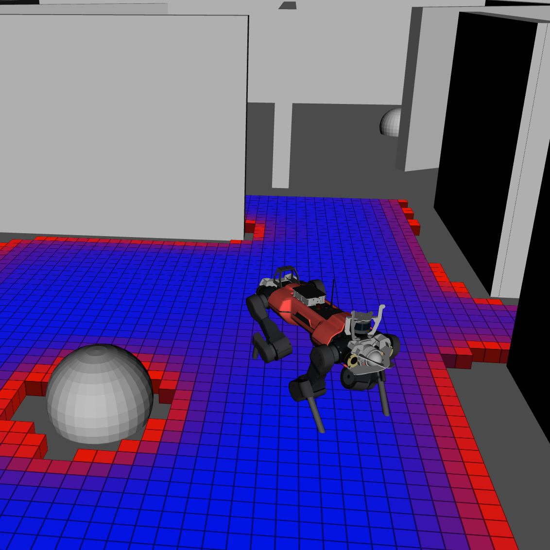
(a) Traversability estimation

(b) Sample environment

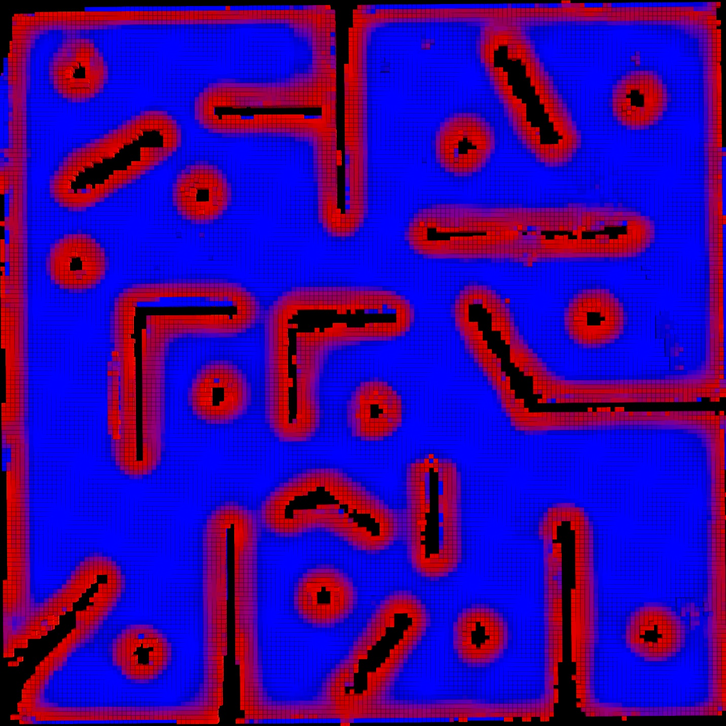
(c) Traversability map

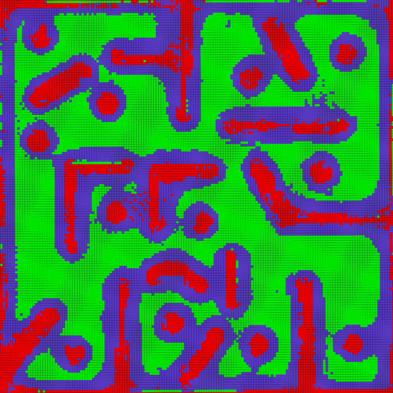
(d) Traversability levels segmentation

Figure 3: (a) The traversability network does not only estimate the traversability for voxels, but it also segments the obstacles out. No traversability voxels are placed around the obstacles, which prevents the planner from sampling here. (b) A sample indoor environment with twelve targets. (c) Traversability map of the sample environment produced with the traversability network, the traversability ranges from $0$ to $1$, colored from red to blue. (d) Segmentation of the traversability map into three levels using $t_{low}=0.3,t_{high}=0.8$. High traversability is marked as green, low traversability as red, and intermediate traversability as purple.

IV-B2 Volumetric Iterative Collision Checking

For the region with unclear traversability, we resort to the iterative volumetric checking for the bounding box of the robot base. The method uses the produced by Voxblox [voxblox] to check if the box is in collision with the environment. To do so, the distance from the box center to the nearest environment surface is obtained from the TSDF map and compared to the box’s outer and inner sphere radius. The box is in collision if the distance is smaller than the inner sphere radius, and not in collision if the distance is larger than the outer sphere radius. Otherwise, no conclusion is reached, and the algorithm divides the current box into two sub-boxes along its longest dimension and performs the same procedure on them until a predefined minimal sub-box resolution is reached and only the outer sphere is evaluated for collision (Fig. 4).

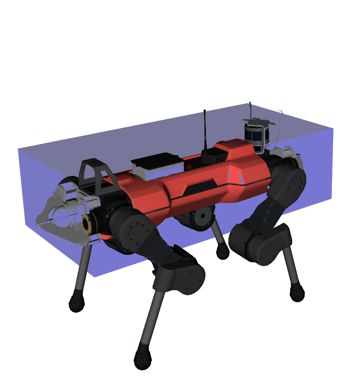
(a) Bounding box

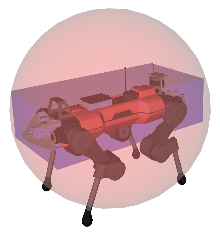
(b) $1$st iteration

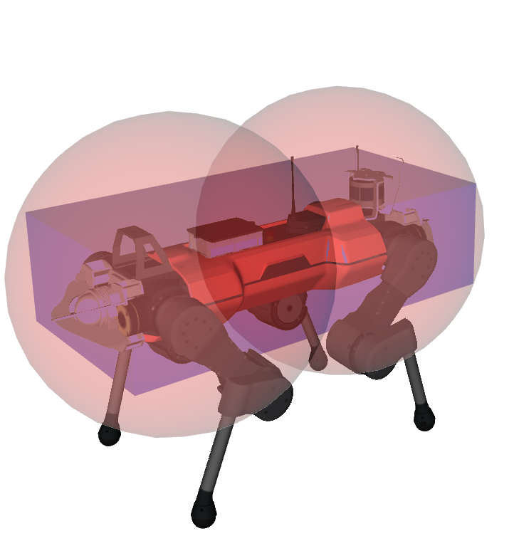
(c) $2$nd iteration

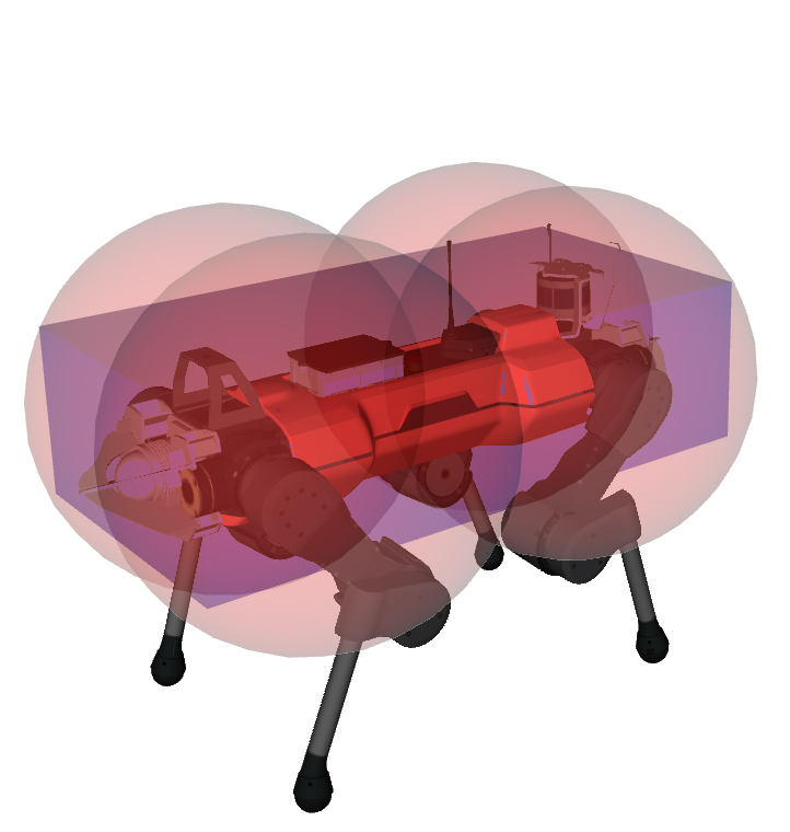
(d) $3$rd iteration

Figure 4: The outer spheres (red) and the bounding box (blue) of the base of the ANYmal robot used in the first three iterations of the volumetric collision checking.

IV-C Optimal Sequencing ()

To find the optimal visiting sequence of the s, we first plan the collision-free paths connecting every pair of s, resulting in the following cost matrix:

$$M=\begin{bmatrix}&0&m_{0,1}&m_{0,2}&\cdots&m_{0,n}\\ &m_{1,0}&0&m_{1,2}&\cdots&m_{1,n}\\ &\vdots&&\ddots&&\vdots\\ &m_{n,0}&m_{n,1}&m_{n,2}&\cdots&0\end{bmatrix},$$ (8)

where $m_{i,j}$ is the cost of the collision-free path from $t_{i}$ to $t_{j}$. For simplicity, we use $t_{0}=s$. This matrix is passed to a TSP solver [google] computing a near-optimal visiting sequence attempting to minimize:

$$\sum_{i=0}^{n-1}m_{\xi_{i},\xi_{i+1}}+m_{\xi_{n},\xi_{0}}$$ (9)

with $\xi_{0}=0$ and $[\xi_{1},\cdots,\xi_{n}]^{\top}$ being a permutation of $[1,\cdots,n]$.

From now on we denote the $i$-th visited as $t_{i}$, where $t_{0}=s$. For each $t_{i}$, we denote the corresponding set of s as $\mathcal{P}_{i}$. The collision-free path connecting two poses $p_{i},p_{j}$ is referred to as $W(p_{i},p_{j})$ in the following.

IV-D Iterative Dynamic Programming

After the visiting sequence is determined, the planner selects the for each . Given all collision-free paths between every of two consecutively visited , i.e. $W(p_{i,j},p_{i+1,k}),\forall{p_{i,j}}\in\mathcal{P}_{i},{p_{i+1,k}}\in\mathcal{P}_{i+1}$, the optimal path cost can be found via by solving the following equations

$$\begin{split}J_{n}^{*}(p_{n,j})={}&Cost(W(p_{n,j},s)),\end{split}$$ (10)

$$\begin{split}J_{i}^{*}(p_{i,j})={}&\min_{p\in\mathcal{P}_{i+1}}Cost(W(p_{i,j},p))+J_{i+1}^{*}(p),\\ &\hskip 100.0pt\forall i\in\left\{1,\cdots,n-1\right\},\end{split}$$ (11)

$$\begin{split}J_{0}^{*}(s)={}&\min_{p\in\mathcal{P}_{1}}{Cost(W(s,p))+J_{1}^{*}(p)}.\end{split}$$ (12)

The optimal s to choose are thus obtained with

$$\begin{split}\hskip 25.0ptp_{0}^{*}={}&s,\end{split}$$ (13)

$$\begin{split}p_{i}^{*}={}&\operatorname*{arg\,min}_{p\in\mathcal{P}_{i}}Cost(W(p^{*}_{i-1},p))+J_{i}^{*}(p),\\ &\hskip 100.0pt\forall i\in\left\{1,\cdots,n\right\}.\end{split}$$ (14)

is guaranteed to output the global optimum given all paths between s of two consecutively visited s. However, in the case of $N$ s and $M$ s per , i.e. $|\mathcal{T}|=N,|\mathcal{P}_{i}|=M$, it requires planning $M^{2}(N-1)+2M$ collision-free paths which increases quadratically with the number of s. Eventually, not every path is used to form the optimal global path. Therefore, we propose to use in an iterative fashion and only plan the collision-free paths if they are needed to construct the optimal global path after each iteration. We define:

$$l(p_{i},p_{j})=\begin{cases}Cost(W(p_{i},p_{j})),&\mbox{if collision-free path }\\ &W(p_{i},p_{j})\mbox{ is planned},\\ c(p_{i},p_{j}),&\mbox{otherwise}.\end{cases}$$ (15)

This is the path cost of the collision-free $W(p_{i},p_{j})$ path between $p_{i}$ and $p_{j}$, if it is already planned. Otherwise, $l(p_{i},p_{j})$ approximates the actual cost of $W(p_{i},p_{j})$ using the straight line between $p_{i}$ and $p_{j}$, i.e. $c(p_{i},p_{j})$ defined in Eq. 4, which is a lower bound of $Cost(W(p_{i},p_{j}))$.

At each iteration, we perform the introduced  (Eqs. 10, 11, 12, 13 and 14), except replacing $Cost(W(\cdot,\cdot))$ by $l(\cdot,\cdot)$, to find the s. Then we generate the collision-free paths connecting the two consecutively visited s and update $l$ accordingly. The algorithm terminates if the selected s do not change over iterations. In this way, not necessarily all $M^{2}(N-1)+2M$ collision-free paths need to be generated, reducing the total planning time.