Bayesian Optimisation of Functions on Graphs

Abstract

The increasing availability of graph-structured data motivates the task of optimising over functions defined on the node set of graphs. Traditional graph search algorithms can be applied in this case, but they may be sample-inefficient and do not make use of information about the function values; on the other hand, Bayesian optimisation is a class of promising black-box solvers with superior sample efficiency, but it has scarcely been applied to such novel setups. To fill this gap, we propose a novel Bayesian optimisation framework that optimises over functions defined on generic, large-scale and potentially unknown graphs. Through the learning of suitable kernels on graphs, our framework has the advantage of adapting to the behaviour of the target function. The local modelling approach further guarantees the efficiency of our method. Extensive experiments on both synthetic and real-world graphs demonstrate the effectiveness of the proposed optimisation framework.

1 Introduction

Data collected in a network environment, such as transportation, financial, social, and biological networks, have become pervasive in modern data analysis and processing tasks. Mathematically, such data can be modelled as functions defined on the node set of graphs that represent the networks. This then poses a new type of optimisation problem over functions on graphs, i.e. searching for the node that possesses the most extreme value of the function. Real-world examples of such optimisation tasks are abundant. For instance, if the function measures the amount of delay at different locations in an infrastructure network, one may think about identifying network bottlenecks; if it measures the amount of influencing power users have in a social network platform, one may be interested in finding the most influential users; if it measures the time when individuals were infected in an epidemiological contact network, an important task would be to identify “patient zero” of the disease.

Optimisation of functions on graphs is challenging. Graphs are an example of discrete domains, and conventional algorithms, which are mainly designed for continuous spaces, do not apply straightforwardly. Real-world graphs are often extremely large and sometimes may not even be fully observable. Finally, the target function, such as in the examples given above, is often a black-box function that is expensive to evaluate at the node level and may exhibit complex behaviour on the graph.

Traditional methods to traverse the graph, such as breadth-first search (BFS) or depth-first search (DFS) [even2011graph], are heuristics that may be adopted in this setting for small-scale graphs, but inefficient to deal with large-scale real-world graphs and complex functions. Furthermore, these search methods only rely on the graph topology and ignore the function on the graph, which can be exploited to make the search more efficient. On the other hand, Bayesian optimisation (BO)  [garnett2023bayesian] is a sample-efficient sequential optimisation technique with proven successes in various domains and is suitable for solving black-box, expensive-to-evaluate optimisation problems. However, while BO has been combined with graph-related settings, e.g. optimising for graph structures (i.e. the individual configurations that we optimise for are graphs) in the context of neural architecture search [kandasamy2018neural, ru2020neural], graph adversarial examples [wan2021adversarial] or molecule design [korovina2020chembo], it has not been applied to the problem of optimising over functions on graphs (i.e. the search space is a graph and the configurations we optimise for are nodes in the graph). The closest attempt was COMBO [oh19combo], which is a framework designed for a specific purpose, i.e. combinatorial optimisation, where the search space is modelled as a synthetic graph restricted to one that can be expressed as a Cartesian product of subgraphs. It also assumes that the graph structure is available and that the function values are smooth in the graph space to facilitate using a diffusion kernel. All these assumptions may not hold in the case of optimisation over generic functions on real-world graphs.

We address these limitations in our work, and our main contributions are as follows: we consider the problem setting of optimising functions that are supported by the node set of a potentially generic, large-scale, and potentially unknown graph – a setup that is by itself novel to the best of our knowledge in the BO literature. We then propose a novel BO framework that effectively optimises in such a problem domain with 1) appropriate kernels to handle the aforementioned graph search space derived by spectral learning on the local subgraph structure and is therefore flexible in terms of adapting to the behaviour of the target function, and 2) efficient local modelling to handle the challenges that the graphs in question can be large and/or not completely known a-priori. Finally, we deploy our method in various novel optimisation tasks on both synthetic and real-world graphs and demonstrate that it achieves very competitive results against baselines.

2 Preliminaries

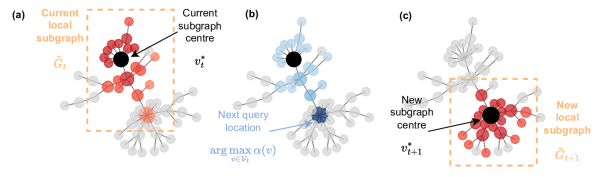
Figure 1: Illustration of one iteration of BayesOptG on an example graph. (a) At iteration $t$, we construct a local subgraph $\tilde{G}_{t}$ centred around $v^{*}_{t}$ whose nodes are marked in orange-red, with darker shade denoting a shorter distance to $v^{*}_{t}$, the best node seen so far (marked in black), and nodes outside $\tilde{G}_{t}$ are marked in grey. The readers are referred to §3.2 for the details; (b) we place a GP surrogate with the covariance function defined in §3.1 on $\tilde{G}_{t}$ and pick the maximiser of the acquisition function (the acquisition function values are marked in shades of blue, with a darker shade denoting a higher acquisition value) as the node to query for iteration $t+1$ ($v_{t+1}$) (§3.2) and (c) if querying $v_{t+1}$ leads to a better objective function value ($f(v_{t+1})<f(v^{*}_{t})$, assuming minimisation), the neighbourhood around it is selected as the new subgraph $\tilde{G}_{t+1}$. The process continues until convergence or a pre-set number of evaluations is reached.

BO is a zeroth-order (i.e. gradient-free) and sample-efficient sequential optimisation algorithm that aims to find the global optimum $x^{*}$ of a black-box function defined over search space $\mathcal{X}$: $x^{*}=\arg\min_{x\in\mathcal{X}}f(x)$ (we consider a minimisation problem without loss of generality). BO uses a statistical surrogate model to approximate the objective function and an acquisition function $\alpha(x)$ to balance exploitation and exploration under the principle of optimism in the face of uncertainty. At the $t$-th iteration of BO, the objective function is queried with a configuration $x_{t}$ and returns an output $y_{t}$, a potentially noisy estimator of the objective function $y_{t}=f(x_{t})+\epsilon,\epsilon\sim\mathcal{N}(0,\sigma_{n}^{2})$ where $\sigma_{n}^{2}$ is the noise variance. The statistical surrogate is trained on the observed data up to $t$-th observation $\mathcal{D}_{t}=\{(x_{i},y_{i})\}_{i=1}^{t}$ to approximate the objective function. In this work, we use a Gaussian process (GP) surrogate, which is query-efficient and gives analytic posterior mean and variance estimates on the unknown configurations. Formally, a GP is denoted as $f(x)\sim\text{GP}\left(m\left({x}\right),k\left({x},{x}^{\prime}\right)\right)$, where $m\left({x}\right)$ and $k\left({x},{x}^{\prime}\right)$ are the mean function and the covariance function (or the kernel), respectively. While the mean function is often set to zero or a simple function, the covariance function encodes our belief on the property of the function we would like to model, the choice of which is a crucial design decision when using GP. The covariance function typically has some kernel hyperparameters $\theta$ and are typically optimised by maximising the log-marginal likelihood (the readers are referred to detailed derivations in rasmussen2004gaussian). With $m(\cdot)$ and $k(\cdot,\cdot)$ defined, at iteration $t$, with $\mathbf{X}_{t}=[x_{1},...,x_{t}]^{\top}$ and the corresponding output vector $\mathbf{y}_{1:t}=[y_{1},...,y_{t}]^{\top}$, a GP gives analytic posterior mean $\mu(x_{t+1}|\mathcal{D}_{t})=\mathbf{k}(x_{t+1},\mathbf{X}_{1:t})\mathbf{K}^{-1}_{1:t}\mathbf{y}_{1:t}$ and variance $k(x_{t+1},x^{\prime}_{t+1}|\mathcal{D}_{t})=k(x_{t+1},x^{\prime}_{t+1})-\mathbf{k}(x_{t+1},\mathbf{X}_{1:t})\mathbf{K}^{-1}_{1:t}\mathbf{k}(\mathbf{X}_{1:t},x^{\prime}_{t+1}))$ estimates on an unseen configuration $x_{t+1}$, where $[\mathbf{K}_{1:t}]_{i,j}=k(x_{i},x_{j})$ is the $(i,j)$-th element of the Gram matrix induced on the $(i,j)$-th training samples by $k(\cdot,\cdot)$, the covariance function. With the posterior mean and variance predictions, the acquisition function is optimised at each iteration to recommend the configuration (or a batch of configurations for the case of batch BO) to be evaluated for the $t+1$-th iteration. For additional details of BO, the readers are referred to frazier2018tutorial.

3 Bayesian Optimisation on Graphs

Problem setting.

Formally, we consider a novel setup with a graph $G$ defined by $(\mathcal{V},\mathcal{E})$, where $\mathcal{V}=\{v_{i}\}_{i=1}^{n}$ are the nodes and $\mathcal{E}=\{{e}_{k}\}_{k=1}^{m}$ are the edges where each edge $e_{k}=\{v_{i^{\prime}},v_{j^{\prime}}\}$ connects nodes $v_{i^{\prime}}$ and $v_{j^{\prime}}$. The topology $G$ may be succinctly represented by an adjacency matrix $\mathbf{A}\in\{0,1\}^{n\times n}$; in our case, $m$ and $n$ are potentially large, and the overall topology is not necessarily fully revealed to the search algorithm at running time. It is worth noting that, for simplicity, we focus on the setup of undirected, unweighted graph where elements of $\mathbf{A}$ are binary and symmetrical (i.e. $A_{ij}=A_{ji}$). Specifically, we aim to optimise the black-box, typically expensive objective function that is defined over the nodes, i.e. it assigns a scalar value to each node in the graph. In other words, the search space (i.e. $\mathcal{X}$ in §2) in our setup is the set of nodes $\mathcal{V}$ and the goal of the optimisation problem is to find the configuration(s) (i.e. $x$ in §2) that minimise the objective function $v^{*}=\arg\min_{v\in\mathcal{V}}f(v)$.

Promises and challenges of BO on graphs.

We argue that BO is particularly appealing under the described setup as (1) it is known to be query-efficient, making it suitable for optimising expensive functions, and (2) it is fully black-box and gradient-free; indeed, we often can only observe inputs and outputs of many real-world functions, and gradients may not even exist in a practical setup. However, there exist various challenges in our setup that make the adaptation of BO highly non-trivial, and despite the prevalence of problems that may be modelled as such and the successes of BO, it has not been extended to the optimisation of functions on graphs. Some examples of such challenges are:

1. Exotic search space. BO is conventionally applied in continuous Euclidean spaces, whereas we focus on discrete graph search spaces. The differences in search space imply that key notions to BO, such as the similarity between two configurations and expected smoothness of objective functions (the latter is often used as a key criterion in selecting the covariance function to use), could differ significantly. For example, while comparing the similarity between two points in a Euclidean space requires only the computation of simple distance metrics (like $\ell_{2}$ distance), careful thinking is required to achieve the same in comparing two nodes in a graph that additionally accounts for the topological properties of the graph.

2. Scalability. Real-world graphs such as citation and social networks can often feature a very large number of nodes while not presenting convenient properties such as the graph Cartesian product assumption in oh19combo to accelerate computations. Therefore, it is a technical challenge to adapt BO in this setting while still retaining computational tractability.

3. Imperfect knowledge on the graph structure. Related to the previous point, it may also be prohibitively expensive or even impossible to obtain perfect, complete knowledge on real-world graphs beforehand or at any point during optimisation (e.g. obtaining the full contact tracing graph for epidemiology modelling); as such, any prospective method should be able to handle the situation where the graph structure is only revealed incrementally, on-the-fly.

Overview of BayesOptG.

To effectively address these challenges while retaining the desirable properties of BO, we propose to extend BO to this novel setup and are, to the best of our knowledge, the first to do so. To achieve that, we propose Bayesian Optimisation on Graphs, or BayesOptG in short, and an illustration of the overall procedure is shown in Fig. 1, and an algorithmic description is available in Algorithm 2. For the rest of this section, we discuss in detail the key components of BayesOptG and how the method specifically addresses the challenges identified above.

[H]

Figure 2: Bayesian Optimisation on Graphs (BayesOptG)

[1] Inputs: Number of random points at initialisation/restart $N_{0}$, total number of iterations $T$, subgraph size $Q$, graph $G=\{\mathcal{V},\mathcal{E}\}$ (whose topology is not necessarily fully known a-priori). Objective: The node $v^{*}_{T}$ that minimises the objective function $f(v),v\in\mathcal{V}$. Initialise restart_flag $\leftarrow$ True, visited nodes $\mathcal{S}\leftarrow\emptyset$, train data $\mathcal{D}_{0}=\emptyset$, $h\leftarrow 1$. $t=1,...,T$ restart_flag Initialise the GP surrogate $\mathcal{D}_{t}$ with randomly selected $N_{0}$ points from $\mathcal{V}_{\backslash\mathcal{S}}$ and their observations $\mathcal{D}_{t}\leftarrow\{v_{i},y_{i}\}_{i=1}^{N_{0}}$. Construct subgraph $\tilde{G}_{t}=\{\tilde{\mathcal{V}}_{t},\tilde{\mathcal{E}}_{t}\}$ around $v^{*}_{t}$ (best node seen from the last restart) (See Algorithm 4 & §3.2). Fit a GP with kernel defined in Table 1 on $\tilde{G}_{t}$ with $\mathcal{D}_{t}$ by optimising log-marginal likelihood. Select next query point $v_{t+1}$ by optimising the acquisition function. Query objective function $f(\cdot)$ at $v_{t+1}$ to obtain a (potentially noisy) estimate $y_{t+1}$; update train data $\mathcal{D}_{t+1}\leftarrow\mathcal{D}_{t}\cup(v_{t+1},y_{t+1})$; seen nodes $\mathcal{S}\leftarrow\mathcal{S}\cup v_{t+1}$; determine the state of restart_flag with the criteria described in §3.2. return node that minimises $f(\cdot)$ from all restarts.

3.1 Kernels for BO on Graphs

Kernel design.

Covariance functions are crucial to GP-based BO. To use BO in our setup, a covariance function that gives a principled similarity measure between two nodes $\{v_{i},v_{j}\}\subseteq\mathcal{V}$ is required to interpolate signals on the graph effectively. In this paper, we study several kernels, including both those proposed in the literature (e.g. the diffusion kernel on graphs and the graph Matérn kernel [borovitskiy21matern]) and two novel kernels designed by us. Following smola2003kernels, all the kernels investigated can be considered in a general formulation. Formally, for a generic graph $\tilde{G}=(\tilde{\mathcal{V}},\tilde{\mathcal{E}})$ with $\tilde{n}$ nodes and $\tilde{m}$ edges, we define $\tilde{\mathbf{L}}:=\frac{1}{2}\Big{(}\mathbf{I}-\tilde{\mathbf{D}}^{-\frac{1}{2}}\tilde{\mathbf{A}}\tilde{\mathbf{D}}^{-\frac{1}{2}}\Big{)}$, where $\mathbf{I}$ is the identity matrix of order $\tilde{n}$, $\tilde{\mathbf{A}}$ and $\tilde{\mathbf{D}}$ are the adjacency matrix and the degree matrix of $\tilde{G}$, respectively (the term after $\frac{1}{2}$ is known as the normalised Laplacian matrix with eigenvalues in the range of $[0,2]$; we scale it such that the eigenvalues are in the range of $[0,1]$). It is worth emphasising that here we use notations with the tilde (e.g., $\tilde{G},\tilde{n}$ and $\tilde{m})$ to make the distinction that this graph is, in general, different from, and is typically a subgraph of, the overall graph $G$ discussed at the start of this section, which might be too large or not be fully available at the start of the optimisation; we defer a full discussion on this in §3.2. We further note that $\tilde{\mathbf{L}}=\mathbf{U}\mathbf{\Lambda}\mathbf{U}^{\top}$ with $\mathbf{\Lambda}=\mathrm{diag}(\lambda_{1},...,\lambda_{\tilde{n}})$ and $\mathbf{U}=[\mathbf{u}_{1},...,\mathbf{u}_{\tilde{n}}]$, where $\{\lambda_{1},...,\lambda_{\tilde{n}}\}$ are the eigenvalues of $\mathbf{\Lambda}$ sorted in an ascending order and $\{\mathbf{u}_{1},...,\mathbf{u}_{\tilde{n}}\}$ are the corresponding (unit) eigenvectors.

Let $p,q\in\{1,...,\tilde{n}\}$ be two indices over the nodes of $\tilde{G}$, we may express our covariance function to compute the covariance between an arbitrary pair of nodes $v_{p},v_{q}$ in terms of a regularisation function of eigenvalues $r(\lambda_{i})\,\forall\,i\in\{1,...,\tilde{n}\}$, as described in smola2003kernels:

$$\small k(v_{p},v_{q})=\sum_{i=1}^{\tilde{n}}r^{-1}(\lambda_{i})u_{i}[p]u_{i}[q],$$ (1)

where $u_{i}[p]$ and $u_{i}[q]$ are the $p$-th and $q$-th elements of the $i$-th eigenvector $\mathbf{u}_{i}$. The specific functional form of $r(\lambda_{i})$ depends on the kernel choice, and the kernels considered in this work are listed in Table 1. We note that all kernels encode the smoothness of the function on the local subgraph $\tilde{G}$. In particular, the diffusion kernel has been adopted in oh19combo; the polynomial and Matérn kernels are inspired by recent work in the literature of graph signal processing [defferrard2016convolutional, zhi2023gaussian, borovitskiy2021matern]; finally, the sum-of-inverse polynomials kernel is designed as a variant of the polynomial kernel: in terms of the regularisation function, it can be interpreted as (while ignoring $\epsilon$) a scaled harmonic mean of the different degree components of the polynomial kernel. We next discuss the behaviours of these kernels from the perspective of kernel hyperparameters.

Table 1: Kernels considered in terms of the regularisation function $r(\lambda_{i})$. We derive the semi-definiteness of polynomial and sum-of-inverse polynomial kernels in App. LABEL:app:semi_definiteness.

Kernel	Regularisation function $r(\lambda_{i})$	Kernel function $K(\mathcal{V},\mathcal{V})$
Diffusion${}^{\dagger}$ [smola2003kernels, oh19combo]	$\exp(\beta_{i}\lambda_{i})$	$\sum_{i=1}^{\tilde{n}}\exp(-\beta_{i}\lambda_{i})\mathbf{u}_{i}\mathbf{u}_{i}^{\top}$
Polynomial${}^{*}$	$\sum_{\alpha=0}^{\eta-1}\beta_{\alpha}\lambda_{i}^{\alpha}+\epsilon$	$\sum_{i=1}^{\tilde{n}}\Big{(}\sum_{\alpha=0}^{\eta-1}\beta_{\alpha}\lambda_{i}^{\alpha}+\epsilon\Big{)}^{-1}\mathbf{u}_{i}\mathbf{u}_{i}^{\top}$
Sum-of-inverse polynomials${}^{*}$	$\Big{(}\sum_{\alpha=0}^{\eta-1}\frac{1}{\beta_{\alpha}\lambda_{i}^{\alpha}+\epsilon}\Big{)}^{-1}$	$\sum_{i=1}^{\tilde{n}}\Big{(}\sum_{\alpha=0}^{\eta-1}\frac{1}{\beta_{\alpha}\lambda_{i}^{\alpha}+\epsilon}\Big{)}\mathbf{u}_{i}\mathbf{u}_{i}^{\top}$
Matérn [borovitskiy21matern]	$\Big{(}\beta\nu+\lambda_{i}\Big{)}^{\nu}$	$\sum_{i=1}^{\tilde{n}}\Big{(}\beta\nu+\lambda_{i}\Big{)}^{-\nu}\mathbf{u}_{i}\mathbf{u}_{i}^{\top}$
${}^{\dagger}$Can be ARD or non-ARD: for ARD, $\{\beta_{i}\}_{i=1}^{\tilde{n}}$ coefficients are learned; for non-ARD, a single, scalar $\beta$ is learned.
${}^{*}$$\{\beta_{\alpha}\}_{\alpha=0}^{\eta-1}$ coefficients to be learned. $\epsilon$: small positive constant (e.g. $10^{-8}$). $\eta$: order of kernel.

Kernel hyperparameters.

$\boldsymbol{\beta}:=[\beta_{0},...,\beta_{\eta-1}]^{\top}\in\mathbb{R}^{\eta}_{\geq 0}$ (for polynomial and sum-of-inverse polynomials) or $[\beta_{1},...,\beta_{\tilde{n}}]^{\top}\in\mathbb{R}^{\tilde{n}}_{\geq 0}$ (for the diffusion kernel) define the characteristics of the kernel. We constrain $\boldsymbol{\beta}$ in both kernels to be non-negative to ensure the positive semi-definiteness of the resulting covariance matrix and are learned jointly via GP log-marginal likelihood optimisation. The parameter $\nu$ controls the mean-square differentiability in the classical GP literature with the Matérn kernel. The polynomial and the sum-of-inverse polynomials kernels in Table 1 feature an additional hyperparameter of kernel order $\ \eta\in\mathbb{Z}_{\geq 0}$. We set it to be $\min\{5,\textit{diameter}\}$ where diameter is the length of the shortest path between the most distanced pair of nodes in $\tilde{G}$ (a thorough ablation study on $\eta$ is presented in App. LABEL:app:ablation.). We argue that this allows both kernels to strike a balance between expressiveness, as all eigenvalues contained in the graphs are used in full without truncation, and regularity, as fewer kernel hyperparameters need to be learned. This is in contrast to, for example, diffusion kernels on graphs in Table 1, which typically has to learn $\tilde{n}$ hyperparameters for a graph of size $\tilde{n}$, whose optimisation can be prone to overfitting. To address this issue, previous works often had to resort to strong sparsity priors (e.g. horseshoe priors [carvalho2009handling]) and approximately marginalising with Monte Carlo samplers that significantly increase the computational costs and reduce the scalability of the algorithm [oh19combo]. In contrast, by constraining the order of the polynomials to a smaller value, the resulting kernels may adapt to the behaviour of the target function and can be better regularised against overfitting in certain problems, as we will validate in §LABEL:sec:experiments.

3.2 Tractable Optimisation via Local Modelling

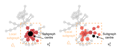
Figure 3: Subgraphs $\tilde{G}_{t}$ determined by Algorithm 4, marked in red, with a darker shade denoting a closer distance to the central node $v^{*}_{t}=\mathop{\arg\min}_{v\in\{v_{t}\}_{t^{\prime}=1}^{t}}f(v)$ in the figure, marked in black), for a high-degree node (Left) and a node far from high-degree node (Right). Note for the latter case, the local subgraph can include nodes that are much further away.

As discussed previously, it is a technical challenge to develop high-performing yet efficient methods in 1) large, real-world graphs (e.g. social network graphs) and 2) graphs for which it is expensive, or even impossible, to obtain complete topological information beforehand (e.g. if we model the interactions between individuals as a graph, the complete topology of the graph may only be obtained after exhaustive interviews and contact tracing with all people involved). The previous work in oh19combo cannot handle the second scenario and only addresses the first issue by assuming a certain structure of the graph (e.g. the Cartesian product of subgraphs), but these techniques are not applicable when we are dealing with a general graph $G$.

[H]

Figure 4: Selecting a local subgraph

[1] Inputs: Best input up to iteration $t$ since the last restart: $v^{*}_{t}$, subgraph size $Q$. Output: local subgraph $\tilde{G}_{t}$ with $Q$ nodes. Initialise: $\tilde{\mathcal{V}}_{t}\leftarrow\{v^{*}_{t}\}$, $h\leftarrow 1$. $|\tilde{\mathcal{V}}_{t}|<Q$ Find $\mathcal{N}_{h}$, the $h$-hop neighbours of $v^{*}_{t}$. $|\tilde{\mathcal{V}}_{t}|+|\mathcal{N}_{h}|\leq Q$ Add all $h$-hop neighbours to $\tilde{\mathcal{V}}_{t}$: $\tilde{\mathcal{V}}_{t}\leftarrow\tilde{\mathcal{V}}_{t}\cup\mathcal{N}_{h}$. Increment $h$: $h\leftarrow h+1$ Randomly sample $Q-|\tilde{\mathcal{V}}|_{t}$ nodes from $\mathcal{N}_{h}$ and add to $\tilde{\mathcal{V}}_{t}$ return the subgraph $\tilde{G}_{t}$ induced by $\tilde{\mathcal{V}}_{t}$ (i.e. the ego-network).