Deep Learning with Partially Labeled Data for Radio Map Reconstruction

Abstract

In this paper, we address the problem of Received Signal Strength map reconstruction based on location-dependent radio measurements and utilizing side knowledge about the local region; for example, city plan, terrain height, gateway position. Depending on the quantity of such prior side information, we employ Neural Architecture Search to find an optimized Neural Network model with the best architecture for each of the supposed settings. We demonstrate that using additional side information enhances the final accuracy of the Received Signal Strength map reconstruction on three datasets that correspond to three major cities, particularly in sub-areas near the gateways where larger variations of the average received signal power are typically observed.

1 Introduction

Retrieving the exact position of the connected objects has become an important feature of the Internet of Things (IoT). Such connected objects have indeed been widespread over the last few years thanks to the low cost of the radio integrated chips and sensors and their possibility of being embedded in plurality of the devices.

By this they can help in fast development of large-scale physical monitoring and crowdsensing systems (like smart cities, factories, transportation, etc.). For the location-dependent application and services these abilities to associate accurate location with physical data gives huge opportunities [25]. For example, the fine-grain and dynamic update of air pollution and/or weather maps could benefit from geo-referenced mobile sensing [1] (e.g., aboard taxis, buses, bicycles…), thus continuously complementing the data from static stations. One of the localization techniques is Global Positioning System (GPS) which has been widely used over the past decades. More recently, low-cost advanced GPS solutions were proposed (like RTK, Bi-band,..), but still they suffer from high energy consumption which is not suitable for IoT applications.

As an alternative, one can opportunistically measure location-dependent radio metrics, like Received Signal Strength (Indicator) (RSSI), Time (Difference) of Arrival, Angle of Arrival, etc., because these sensor nodes communicate with one/several gateways at the same time (e.g. while sending a packet to the infrastructure to store this data in the cloud/server). Based on these metrics, there exist several methods to determine the node position: trilateration, triangulation, proximity detection, or fingerprinting [60, 13, 9]. We will focus on the last approach – fingerprinting [10]– which requires (ideally) full map of mentioned above radio metrics, covering the zone of interest. However, collecting metrics in each point of the zone of interest is impractical and time costly in real-world scenarios, therefore most approaches rely on sparse and non-uniformly distributed measurements.

In this sense, classical map interpolation techniques such as RBF [47, 42, 16] or kriging [41, 32] are used. Although these methods are relatively fast, they are quite weak in retrieving and predicting the complex and heterogeneous spatial patterns that are usually observed in real life signals (e.g., sudden and/or highly localized transient variations in the received radio metric due to specific environmental, local or topological effects). Another approach consists on deterministic simulation such as Ray-Tracing tools [8, 28, 44, 54]. Given some real field measurements and then calibrated over them, these models predict the radio propagation while simulating electromagnetic interactions with the environment. These technologies, however, need a complete description of the environment (properties of the materials of the obstacles, buildings, shape,etc.). Moreover, they are computationally complex, and in case of minor changes in the local area, these simulations should be re-run again. Recently, studies have employed machine learning for this task by considering radio maps as images and adapting neural network models that have been proposed for image completion. These models are based on the fully generated dataset by Ray-Tracing tools for predicting the signal propagation given the buildings mask and position of the transmitter [29]; or predicting the received power value for the Long Term Evolution (LTE) of the signal with use of additional information and neural networks [21, 39] with handcrafted structures.

In this work we will focus on the received signal strength map reconstruction, where only small amount of ground truth GPS-tagged measurements are available preventing to use existing NN models with handcrafted architectures and for which Ray-Tracing models could not be applied due to the lack of information about physical properties of the environment or due to high computational complexity. Our approach is based on Neural Architecture Search (NAS) [15] which aims to find an optimized NN model for this task. We show that by employing the latter technique, it is feasible to learn model parameters while simultaneously exploring the architecture. In addition, we employ unlabeled data in conjunction with ground-truth measurements in the training phase, as well as side information that accounts for the existence of buildings, to obtain knowledge and improve the model’s performance. We assess our technique using three RSSI Map reconstruction collections, including one we produced for the city of Grenoble in France. In the case of the latter, we thoroughly examine its properties. In particular, we show that unlabeled data can effectively be used to find an efficient optimized NN model and that the side information provides valuable knowledge for learning. The obtained model is shown to have generalization ability on base stations that were not used in the training phase. The contribution of this paper is twofold:

• We propose a unified framework with the use of side information, for which we study the generalization ability of a neural network model which architecture is optimized over labeled and unlabeled data using side-information. This is an extension of the work of [37, 36].

• Furthermore, we provide empirical evaluation over three large-scale RSSI collections showing that the proposed approach is highly competitive compared to the state-of-the-art models in terms of quality metrics.

2 Related State of the Art

Classical techniques such as radial basis functions (RBF) or kriging [10] are simple and fast, but they are poor at predicting the complex and heterogeneous spatial patterns commonly observed in real-world radio signals (e.g., sudden and/or highly localized transient variations in the received signal due to specific environmental or topological effects, such as specific building shapes, presence of public furniture, ultra-navigation, etc.). Furthermore, data augmentation approaches for artificially increasing the number of measurements in radio map reconstruction issues have been developed.

The goal is to use the synthetic data created as extra data to train complex map interpolation models. However, these techniques need a highly thorough description of the physical environment and are unable to predict dynamic changes in the environment over time. A key bottleneck is their high computational complexity.

In the following, we go through some more relevant work on RSSI map reconstruction, including interpolation and data-augmentation techniques, as well as machine learning approaches.

2.1 Interpolation and data-augmentation techniques

Kriging or Gaussian process regression [30] is a prominent technique for radio map reconstruction in the wireless setting that takes into consideration the distance information between supplied measured locations while attempting to uncover their underlying 2D dependency.

Radial basis functions (RBF) [10, 16, 47] are another approach that simply considers the dependent on the distance between observed locations. As a result, this method is more adaptive and has been found to be more tolerant to some uncertainty [50]. Furthermore, in order to compare the performance of the RBF with different kernel functions for the map reconstruction of signal strength of LoRa radio waves, [10] divided all of the points in a database of outdoor RSSI measurements into training and testing subsets, with the linear kernel showing the best accuracy in both standard deviation and considered metric. The two approaches stated above (which depend on kernel techniques and underlying spatial relationships of the input measurements) need a lot of input data to provide reliable interpolation results, making them sensitive to sparse training sets. These methods have consequently been considered in pair with crowdsensing, where, for example in [32], to improve the performance of basic kriging, one calls for measuring the radio metric in new points/cells where the predicted value is still presumably imprecise. A quite similar crowdsensing method has also been applied in [18] after considering the problem as a matrix completion problem using singular value thresholding, where it is possible to ask for additional measurements in some specific cells where the algorithm has a low confidence in the predicted result. In our case though, we assume that we can just rely on a RSSI map with few ground-truth initial RSSI measurements.

Another approach considered in the context of indoor wireless localization (with map reconstruction firstly) relies on both measured field data and an a priori path loss model that accounts for the effect of walls presence and attenuation between the transmitter and the receiver [26] by using the wall matrix, which counts the number of walls along the path from the access point to the mobile location and penalize value according to that number. In some outdoor settings, training points are divided into a number of clusters of measured neighbors having specific RSSI distributions, and local route loss models are applied in an effort to capture localized wireless topology effects in each cluster [40]. However as parametric path loss models are usually quite imprecise, these techniques have a limited generalization capabilities and require additional impractical in-site (self-)calibration. A quite similar approach, except the use of additional side information, is followed in [33], where they propose an algorithm called SateLoc. Based on satellite images, it is then suggested to perform a segmentation of the areas “crossed” by a given radio link, depending on their type (e.g., terrain, water, forest, etc.). Then, proportionally to the size of the crossed region(s), power path loss contributions are computed according to a priori model parameters (i.e., associated with each environment type) and summed up to determine the end-to-end path loss value.

One more way to build or complete radio databases stipulated in the context of fingerprinting based positioning consists in relying on deterministic simulation approach, namely Ray-Tracing tools (e.g., [44, 45, 53, 54, 28]). This technique aim at predicting in-site radio propagation (i.e., simulating electromagnetic interactions of transmitted radio waves within an environment). Once calibrated with a few real field measurements, such simulation data can relax initial metrology and deployment efforts (i.e., the number of required field measurements) to build an exploitable radio map, or even mitigate practical effects that may be harmful to positioning, such as the cross-device dispersion of radio characteristics (typicaly, between devices used for offline radio map calibration and that used for online positioning). Nevertheless, these tools require a very detailed description of the physical environment (e.g., shape, constituting materials and dielectric properties of obstacles, walls…). Moreover, they are notorious for requiring high and likely prohibitive computational complexity in real applications. Finally, simulations must be re-run again, likely from scratch, each time minor changes are introduced in the environment, e.g. the impact of human activity (like changing crowd density, temporary radio link obstructions).

2.2 NN based models trained after data augmentation

There is more and more interest in application of machine and deep learning methods to the problem of RSSI map reconstruction. These approaches have shown an ability to capture unseen spatial patterns of local effects and unseen correlations. Until now, to the best of our knowledge, these algorithms were primarily trained over simulated datasets generated by data-augmentation approaches (that were mentioned above).

In [29], given a urban environment, city geography, Tx location, and optionally pathloss measurements and car positions the authors introduce a UNet-based neural network called RadioUNet in the supervised learning setting, which outputs radio path loss estimates trained on a large set of generated using the Dominant Path Model data [48].

[20] propose a two-phase transfer learning with Generative Adversarial Networks (GAN), which comprises of two stages, to estimate the power spectrum maps in the underlay cognitive radio networks. The domain projecting (DP) framework is used to first project the source domain onto a neighboring domain. The target domain’s entire map is then rebuilt or reconstructed using the domain completing framework and the recovered features from the surrounding domain.

For training of the DP, fully known signal distribution maps have been used. In another contribution, to improve the kriging predictions the authors have used the feedforward neural network for path loss modelling  [51], as conventional parametric path loss models has a small number of parameters and do not necessarily consider shadowing besides average power attenuation.

Apart from wireless applications, similar problems of map reconstruction also exist in other domains. In [63] for instance, the goal is to create the full topographic maps of mountains area given sparse measurements of the altitudes values. For this purpose, they use a GAN architecture, where in the discriminator they compare pairs of the input data and the so-called “received” map, either generated by the generator or based on the given full true map. In other work [61] the authors estimate the sea surface temperature with use of GAN architecture in the unsupervised settings but having a sequence of corrupted observations (with different clouds coverage) and known mask distribution. Another close more general problem making extensive use of neural networks is the image inpainting problem, where one needs to recover missing pixels in a single partial image. By analogy, this kind of framework could be applied in our context too, by considering the radio map as an image, where each pixel corresponds to the RSSI level for a given node location. It has been shown in [37] the interpretation of collected measurements on a map as an image with some pixels gives overall better result. But the problem is in consumed time as it does not give the generalized model and do not use the additional information about the local environment. Usually, such image inpainting problems can be solved by minimizing a loss between true and estimated pixels, where the former are artificially and uniformly removed from the initial full image. This is however not possible and not realistic in our case, as only a few ground-truth field measurements collected on the map can be used to reconstruct the entire image.

In contrast to the previous approaches, in our study, we consider practical situations where data-augmentation techniques cannot be used, mainly because of unknown environment characteristics and computational limitations, and where only a small amount of collected ground-truth measurements is available.

Finally, a few contributions aim at predicting the received power value based on neural networks and additional information. For instance, in [21, 39, 23], RSS values are predicted in exact points, given meta information such as the radio characteristics (e.g., transmission specifications or relationship between Rx and Tx, like horizontal/vertical angle, mechanical/electrical tilt angle, 2D/3D distance, base station antenna orientation, etc.) and/or prior information about the buildings (e.g., height and presence). In case the latter information is missing, predictions can be made also by means of satellite images (e.g., paper [23]). In these papers though, the map reconstruction cannot be performed directly. As the prediction is realized for each point separately, it is thus time consuming. Moreover, the authors do not take into account the local signal values, but only the physical parameters and physical surroundings (similarly to standard path loss models).

2.3 Neural Architecture Search

The creation and selection of features in many tasks are done manually in general; this critical phase for some conventional machine learning algorithms might be time-consuming and costly. Neural Networks address this challenge by learning feature extractors in an end-to-end manner. These feature extractors, on the other hand, rely on architectures that are still manually constructed, and with the rapid development of the field, designing an appropriate NN model has become onerous in many cases.

This problem has recently been addressed by a new field of research called (NAS) [15]. In a variety of applications, such as image segmentation and classification, Neural Networks with automatically found architectures have already outperformed “conventional” NN models with hand-crafted structures.

Different types of existing methods of search are described below. In the last few years the research on the topic of NAS has been shown a huge interest in the different fields. Among various studies, there are different techniques that are based on divers methods like Reinforcement Learning [64], Evolutionary Algorithm [46] or Bayesian Optimization [24]. Lately, recent gradient-based methods became more and more popular. For example, one of the first methods based on this technique was presented in [35] ans is called DARTS, which is using relaxation to, at the same time, optimize the structure of a cell, and the weight of the operations relative to each cell. After finding the best combinations, blocks are stacked manually to produce a neural network. Based on DARTS, more complex methods have appeared such as AutoDeepLab [34] in which a network is optimized at 3 levels : $(i)$ the parameters of the operations, $(ii)$ the cell structure and $(iii)$ the macro-structure of the network that is stacked manually. Despite the fact that a complex representation leads to powerful architectures, this technique has some drawbacks, such as the fact that the generated architecture is single-path, which means it does not fully exploit the representation’s capabilities. Moreover, as the search phase is done over a fixed network architecture, it might not be the same between different runs, thus it is complicated to use transfer learning and the impact of training from scratch can be significant. To overcome these limitations, one possible technique is to use Dynamic Routing as proposed in [31]. This approach is different from the traditional gradient based methods proposed for NAS in the sense that it does not look for a specific fixed architecture but generates a dynamic path in a mesh of cells on the fly without searching by weighting the paths during training procedure.

In the topic of signal strength map reconstruction there was no studies (for our knowledge) with application of NAS to the field measurements.

In our study, we look at how well neural networks can extract complex features and their relationships to signal strength in the local area or under similar conditions, as well as their ability to take into account additional environmental information without having access to more complex physical details. This is performed through a search for a model with an optimized architecture adapted to the task. For this we consider the genetic algorithm of architecture search as it has been shown in [37] that it outperforms the dynamic routing search.

2.4 Semi-Supervised Learning

The constitution of coherent and consistent labeled collections are often done manually. This necessitates tremendous effort, which is generally time consuming and, in some situations, unrealistic. The learning community has been looking at the concept of semi-supervised learning for discrimination and modeling tasks since the end of the 1990s, based on the observation that labeled data is expensive while unlabeled data is plentiful and contains information on the problem we are trying to solve.

Framework and definitions

In this case, the labeled examples are generally assumed to be too few to obtain a good estimate of the association sought between the input space and the output space and the aim is to use unlabeled examples in order to obtain a better estimate. For this, we will assume available a set of labeled training examples $S=\{(x_{i},y_{i})\mid i=1,\ldots,m\}\in(\mathcal{X}\times\mathcal{Y})^{m}$ supposed to be generated i.i.d. from an underlying distribution $\mathcal{D}$; and a set of unlabeled examples $X_{u}=\{x_{i}\mid i=m+1,\ldots,m+u\}$ that are drawn i.i.d. from the marginal distribution $\mathbb{P}(x)$. If $X_{u}$ is empty, we fall back on the problem of supervised learning. If $S$ is empty, we deal with an unsupervised learning problem. During learning, semi-supervised algorithms estimate labels for unlabeled examples. We note $\tilde{y}$ the pseudo-label of an unlabeled example $x\in X_{u}$ estimated by these algorithms. The interest of semi-supervised learning arises when $u=|X_{u}|\gg m=|S|$ and the goal is that the knowledge one gains about the marginal distribution, $\mathbb{P}(x)$, through the unlabeled examples can provide information useful in inferring $\mathbb{P}(y\mid x)$. If this goal is not achieved, semi-supervised learning will be less efficient than supervised learning and it may even happen that the use of unlabeled data degrades the performance of the learned prediction function [62, 12, 56]. It is then necessary to formulate working hypotheses for taking unlabeled data into account in the supervised learning of a prediction function.

Inductive vs Transductive Learning

Before presenting these hypotheses, we note that semi-supervised learning can be formulated in two different possible settings, namely transductive and inductive learning. The aim in inductive case is to minimize the generalization risk with respect to the distribution $\mathcal{D}$, by training a model over a finite number of training samples [59]. This setting is also the most common in semi-supervised learning.

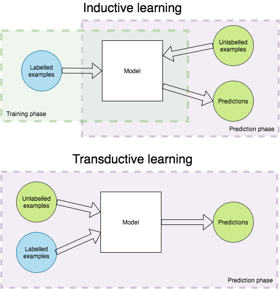
Figure 1: Inductive and transductive learning. In inductive learning there are two separate stages of training and prediction, while in transductive learning there is only one and which is prediction.

Despite this, accurate predictions for only the unlabeled cases in $X_{u}$ are more crucial in some applications than finding a more general rule for all existing examples drawn i.i.d. with respect to $\mathcal{D}$. It was shown in [57, 58] that in this scenario, it would be preferable to ignore the more general problem and concentrate on an intermediary problem known as transductive learning [19]. As a result, rather than looking for a general rule first (as in inductive learning), the goal of learning in this situation would be to predict the class labels of unlabeled cases by having the smallest average error (called the transductive error). These two settings are depicted in Figure 1.

Central assumptions

The three major hypotheses in SSL that are: smoothness assumption, cluster assumption and manifold assumption.

The basic assumption in semi-supervised learning, called the smoothness assumption states that:

$\mathcal{H}_{1}$: If two examples $x_{1}$ and $x_{2}$ are close in a high density region, then their class labels $y_{1}$ and $y_{2}$ should be similar.

This assumption implies that if two points belong to the same group, then their output label is likely to be the same. If, on the other hand, they were separated by a low density region, then their outputs would be different.

Now suppose that the examples of the same class form a partition. The unlabeled data could then help find the boundary of each partition more efficiently than if only the labeled examples were used. So one way to use the unlabeled data would be to find the partitions with a mixture pattern and then assign class labels to the partitions using the labeled data they contain. The underlying hypothesis of the latter, called the cluster assumption, can be formulated by:

$\mathcal{H}_{2}$: If two examples $x_{1}$ and $x_{2}$ are in the same group, then they are likely to belong to the same class $y$.

This hypothesis could be understood as follows: if there is a group formed by a dense set of examples, then it is unlikely that they can belong to different classes. This is not equivalent to saying that a class is formed by a single group of examples, but that it is unlikely to find two examples belonging to different classes in the same group. According to the previous continuity hypothesis, if we consider the partitions of examples as regions of high density, another formulation of the partition hypothesis is that the decision boundary passes through regions of low density. This assumption is the basis of generative and discriminative methods for semi-supervised learning.

For high-dimensional problems, these two hypotheses may not be accurate since the search for densities is often based on a notion of distance which loses its meaning in these cases. A third hypothesis, called the manifold assumption, on which some semi-supervised models are based, then stipulates that:

$\mathcal{H}_{3}$: For high-dimensional problems, the examples are on locally Euclidean topological spaces (or geometric manifolds) of low dimension.

In the following, we will present some classic models of the three families of semi-supervised methods resulting from the previous hypotheses.

There are three main families of SSL approaches that have been developed according to the above assumptions.

Generative Methods

Semi-supervised learning with generative models involves estimating the conditional density $\mathbb{P}(x\mid y,\Theta)$ using a maximum liklihood technique to estimate the parameters $\Theta$ of the model. In this case, the hidden variables associated with the labeled examples are known in advance and correspond to the class of these examples. The basic hypothesis of these models is thus the cluster assumption (Hypothesis $\mathcal{H}_{2}$) since, in this case, each partition of unlabeled examples corresponds to a class [52]. We can thus interpret semi-supervised learning with generative models $(a)$ as a supervised classification where we have additional information on the probability density $\mathbb{P}(x)$ of the data, or $(b)$ as a partition with additional information on the class labels of a subset of examples [5, 38]. If the hypothesis generating the data is known, generative models can become very powerful [62].

Discriminant Methods

The disadvantage of generative models is that, in the case where the distributional assumptions are no longer valid, their use will tend to deteriorate their performance compared to the case where only labeled examples are employed to learn a model [11]. This finding has motivated many works to overcome this situation. The first works were based on the so-called directed decision technique (or self-training) proposed in the context of the adaptive processing of the signal and which consists in using the current predictions of the model for unlabeled examples in order to assign them pseudo-labels and use the pseudo-labeled examples in the training process. This process of pseudo-labeling and learning is repeated until no more unlabeled examples are pseudo-labeled. In the case where class pseudo-labels are assigned to unlabeled examples, by thresholding the outputs of the classifier corresponding to these examples, it can be shown that the self-learning algorithm works according to the clustering assumption [4].

Graph-based Methods

Generative and discriminant methods proposed in semi-supervised learning exploit the geometry of the data through density estimation techniques or based on the predictions of a learned model. The last family of semi-supervised method uses an empirical graph $G=(V,E)$ built on the labeled and unlabeled examples to express their geometry. The nodes $V=[1,\ldots,m+u]$ of this graph represent the training examples and the edges $E$ translate the similarities between the examples. These similarities are usually given by a positive symmetric matrix $\boldsymbol{W}=[W_{ij}]_{i,j}\in\mathbb{R}^{(m+u)\times(m+u)}$, where the weight $W_{ij}$ is non-zero if and only if te examples indices $i$ and $j$ are connected, or equivalently, if $(i,j)\in E\times E$ is an edge of the graph $G$.

3 Application to the Stated RSS Map Reconstruction Problem

Additional information could be represented in different manners, and they could be included into the algorithm in a variety of ways, such as independent channels, parallel channels inputs, directly in the learning goal, or in the ranking metric during model selection. We adapted the proposed algorithm presented in [36] for multi-channel input by combining additional context information with the data in the model’s input; and we assessed the model’s performance on unseen base stations that were not utilized in the learning process.

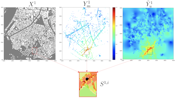
Figure 2: An example of constituting the training sets for one base station. $X^{1}$ corresponds to 2D node locations, buildings are shown in white. $Y_{m}^{1}$ is RSSI map (true measurements); the base station is shown by a black circle,and $\tilde{Y}^{1}$ corresponds to interpolated points found by RBF. Colors depict the strength of the signal from dark red (highest) to deep blue (lowest) RSSI values. $S^{1,i}=S^{j,i}_{\ell}\cup S^{j,i}_{v}\cup S^{j,i}_{u\!\!\!\backslash}$ is one sub-matrix of partially labeled training data found from $Y_{m}^{1}\cup\tilde{Y}^{1}$.

Here, we suppose to have a small set of $n$ available base stations $(X^{j})_{1\leqslant j\leqslant n}$. For each given matrix of base station $X^{j};j\in\{1,\ldots,n\}$, let $Y^{j}\in\mathbb{R}^{H\times W}$ be its corresponding 2D matrix of signal strength values measurements, where $H\times W$ is the size (in number of elements in a grid) of the zone of interest. In practice, we have access only to some ground truth measurements $Y^{j}_{m}$, meaning that $Y^{j}_{m}=~{}Y^{j}\odot M^{j}$, with $M^{j}\in\{0,1\}^{H\times W}$ a binary mask of available measurements, and $\odot$ is the Hadamard’s product. Here we suppose sparsity meaning that the number of non-null elements in $Y^{j}_{m}$ is much lower than the overall size $H\times W$. For each base station $X^{j}$ we estimate unknown measurements $\tilde{Y}_{u}^{j}$ in $Y^{j}$ with a RBF interpolation given $(X^{j}_{m},Y^{j}_{m})$, so that we have a new subset $(X^{j}_{u},\tilde{Y}^{j}_{u})$, where $X^{j}_{m}=X^{j}\odot M^{j}$ is the associated 2D node locations of $Y^{j}_{m}$ in $X^{j}$, and the values in $\tilde{Y}^{j}_{u}$ are initially given by RBF predictions on $X^{j}_{u}$ corresponding to the associated 2D node locations (or equivalently, the cell/pixel coordinates) with respect to the base station $X^{j}$ which do not have measurements. In our semi-supervised setting, the values for unknown measurements in $\tilde{Y}^{j}_{u}$ will evolve by using the predictions of the current NN model during the learning process.

We further decompose the measurements set $Y^{j}_{m}$ into two parts: $Y^{j}_{\ell}$ (for training), $Y^{j}_{v}$ (for validation), such that $Y^{j}_{\ell}\oplus Y^{j}_{v}=~{}Y^{j}_{m}$, where $\oplus$ is the matrix addition operation. Let $X^{j}_{\ell},X^{j}_{v}$ be the associated 2D node locations pf $Y^{j}_{\ell}$ and $Y^{j}_{v}$ in $X^{j}$.

In our experiments the number of base stations $n$ is small, so in order to increase the size of labeled and pseudo-labeled training samples, we cut the initial measurements maps $(Y_{m}^{j}\oplus\tilde{Y}^{j}_{u})_{1\leqslant j\leqslant n}$ into smaller matrices which resulted into the sets $(S^{j,i})_{\begin{subarray}{c}1\leqslant j\leqslant n\\ 1\leqslant i\leqslant m_{j}\end{subarray}}$ where the sets $S^{j,i}\subseteq Y_{m}^{j}\oplus\tilde{Y}^{j}_{u};\forall i\in\{1,\ldots,m_{j}\}$ are shifted with overlapping of the points. Each submatrix $S^{j,i}$ is hence divided into labeled, $S^{j,i}_{\ell}\cup S^{j,i}_{v}$, and pseudo-labeled (first interpolated points using RBF and then using the predictions of the current NN model) $S^{j,i}_{u\!\!\!\backslash}$. To each submatrix $S^{j,i}$ corresponds a 2D location $X^{j,i}\subset X$. Figure 2 gives a pictorial representation of the notations.

4 NAS with Genetic Algorithm for RSSI map reconstruction using side information

UNet [49] is one of the mostly used primary Neural Network models that can handle multiple channels and hence consider side-information as well as the RSSI map on their input. As additional context (or side) information, we have considered:

• information about buildings presence, which was taken from the open-source OpenStreetMap dataset [7] – matrix of binary 0-1 values, denoted as “buildings map” further (Figure 2 left);

• amount of crossed buildings by signal from base station to each point of the map. By analogy to the data representation in the indoor localisation and map reconstruction, with the amount of crossed walls by signal – matrix of non-negative integer values, denoted as “buildings count map” further;

• information about distance from the base station. By the log-normal path loss model and corresponding RSSI ([43]: the signal strength is proportional to $-10n\log_{10}(d)$ up to additive term, where $n$ is a path loss exponent, $d$ is a distance to base station) we can take the $-\log_{10}(distance)$ transformation to emphasize the zones closest from the base station – matrix of continuous values, denoted as “distance map” further;

• information about the relief represented by DSM (digital surface model): terrain elevation summed with artificial features of the environment (buildings, vegetation..), see Figure 3. This information was taken from the open-source dataset provided by Japan Aerospace Exploration Agency with $30m$ accuracy – matrix of integer values, denoted as “elevation map” further.

  

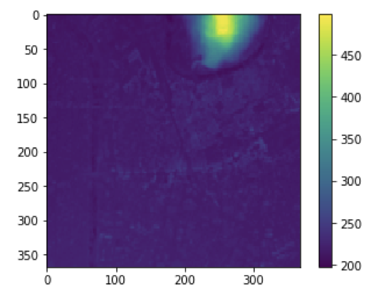
  (a) Elevations map, Grenoble

  

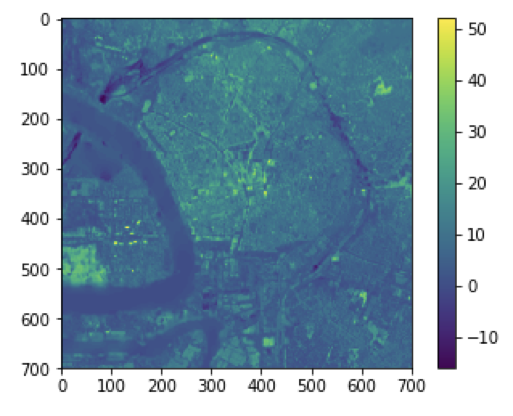
  (b) Elevations map, Antwerp

  Figure 3: Elevation maps for two different cities

Our objective is to find the optimal architecture for UNet using these side-information and study the generalization ability of obtained models for RSSI map reconstruction.

NAS is performed with a Genetic algorithm is similar to one presented in [37] as it gave better performance result in terms of obtained accuracy.

From the sets $(S^{j,i})_{\begin{subarray}{c}1\leqslant j\leqslant n\\ 1\leqslant i\leqslant m_{j}\end{subarray}}$ we use an evolutionary algorithm similar to [46] for searching the most efficient architecture represented as a Direct Acyclic Graph. Here, the validation sets $(S^{j,i}_{v})_{\begin{subarray}{c}1\leqslant j\leqslant n\\ 1\leqslant i\leqslant m_{j}\end{subarray}}$ are put aside for hyperparameter tuning. The edges of this DAG represent data flow with only one input for each node, which is a single operation chosen among a set of candidate operations. We consider usual operations in the image processing field, that are a mixture of convolutional and pooling layers. We also consider three variants of 2D convolutional layers with kernels of size 3, 5 and 7, and two types of pooling layers that compute either the average or the maximum on the filter of size 4.

Candidate architectures are built from randomly selected operations and the corresponding NN models are trained over the set $(S^{j,i}_{\ell})_{\begin{subarray}{c}1\leqslant j\leqslant n\\ 1\leqslant i\leqslant m_{j}\end{subarray}}$ and its (possible) combinations with side information. The resulted architectures are then ranked according to pixel-wise error between the interpolated result of the outputs over $(S^{j,i}_{v})_{\begin{subarray}{c}1\leqslant j\leqslant n\\ 1\leqslant i\leqslant m_{j}\end{subarray}}$ and interpolated measurements given by RBF interpolation by filtering out the buildings. As error functions, we have considered the Mean Absolute Error (MAE) or its Normalized version (NMAE) where we additionally weight the pixel error according to the distance matrix value. Best ranked model is then selected for mutation and placed in the trained population. The oldest and worst in the rank are then removed to keep the population size equal to 20 models.

Once the NN model with the optimized parameters are found by NAS, $f_{\theta}$, we consider the following two scenarios for learning its corresponding parameters $\theta$ by minimizing

$$\mathcal{L}(f_{\theta},S_{\ell}\cup S^{j,i}_{u\!\!\!\backslash})\!=\!\frac{1}{n}\sum_{j=1}^{n}\frac{1}{m_{j}}\sum_{i=1}^{m_{j}}\left[\frac{1}{|S^{i,j}_{\ell}|}\!\!\sum_{(x,y)\in S^{i,j}_{\ell}}\!\!\!\!\ell(y,f_{\theta}(x))\right.\\ \left.+\frac{1}{|S^{j,i}_{u\!\!\!\backslash}|}\sum_{(x,\tilde{y})\in S^{j,i}_{u\!\!\!\backslash}}\ell(\tilde{y},f_{\theta}(x))\right]$$ (1)

These two scenarios relate to obtaining model parameters on labeled and pseudo-labeled measurements using just RBF interpolated data (scenario 1) or predictions from a first model learnt on these data (scenario 2). The overall learning process is depicted in Algorithm 1.

Input: A labeled training set with given measurements: $(X^{j}_{m},Y^{j}_{m})_{1\leqslant j\leqslant n}$ and an unlabeled set $(X_{u}^{j})_{1\leqslant j\leqslant n}$

Init: Using $(X^{j}_{m},Y^{j}_{m})_{1\leqslant j\leqslant n}$, find interpolated measurements $(\tilde{Y}^{j}_{u})_{1\leqslant j\leqslant n}$ over $(X_{u}^{j})_{1\leqslant j\leqslant n}$ using the RBF interpolation method;

Step 1: Cut the initial measurements maps $(Y_{m}^{j}\oplus\tilde{Y}^{j}_{u})_{1\leqslant j\leqslant n}$ into smaller matrices: $(S^{j,i})_{\begin{subarray}{c}1\leqslant j\leqslant n\\ 1\leqslant i\leqslant m_{j}\end{subarray}}$.

Step 2: Search the optimal NN architecture using $(S^{j,i})_{\begin{subarray}{c}1\leqslant j\leqslant n\\ 1\leqslant i\leqslant m_{j}\end{subarray}}$;

Scenario 1: Find the parameters $\theta^{\star}_{1}$ of the NN model $f_{\theta}$ :

$\theta^{\star}_{1}=\mathop{\operatorname*{argmin}}_{\theta}\mathcal{L}(f_{\theta},S_{\ell}\cup S^{j,i}_{u\!\!\!\backslash})$    # (Eq. 1);

Scenario 2: Apply $f_{\theta^{\star}_{1}}$ on unlabeled data and obtain new pseudo-labeled measurements $S^{j,i}_{u\!\!\!\backslash}$ and find the new parameters $\theta^{\star}_{2}$ of the NN model $f_{\theta}$ :

$$\theta^{\star}_{2}=\mathop{\operatorname*{argmin}}_{\theta}\mathcal{L}(f_{\theta},S_{\ell}\cup S^{j,i}_{u\!\!\!\backslash})$$

Output: $f_{\theta^{\star}_{1}}$ for scenario 1 or $f_{\theta^{\star}_{2}}$ for scenario 2.

Algorithm 1 SL${}_{\texttt{NAS}}$^ind

5 Evaluation Setup

We have considered three case studies from Paris, Antwerp (The Netherlands) and Grenoble. In the area of data-based research and in the field of machine learning singularly, it is usually hard to find large open-source datasets made of real data. In some works however, alternatively (or as a complement) to using real data, synthetic data can be generated, for instance through deterministic simulations.

In our study, we make use of three distinct databases of outdoor RSSI measurements with respect to multiple base stations. The first one was generated through a Ray-Tracing tool in the city of Paris, France. The second database, which is publicly available (See [2]), consist of real GPS-tagged LoRaWAN measurements that were collected in the city of Antwerp (The Netherlands). Finally, a third database, which is also made of real GPS-tagged LoRaWAN measurements, was specifically generated in the city of Grenoble (France), in the context of this study.

5.1 Paris dataset

This first dataset is made of synthetic outdoor RSSI measurements, which were simulated in a urban Long Term Evolution (LTE) cellular context with a ray-tracing propagation tool named VOLCANO (commercialized by SIRADEL). Those simulations were calibrated by means of side field measurements [8]. This kind of deterministic tool makes use of both the deployment information (typically, the relative positions of mobile nodes and base stations) and the description of the physical environment (i.e., a city layout with a faceted description of the buildings, along with their constituting materials) to predict explicitly the electromagnetic interactions of the multipath radio signal between a transmitter and a receiver. Beyond the main limitations already mentioned in section 2.1 regarding mostly computational complexity and prior information, we acknowledge a certain number of discrepancies or mismatches in comparison with the two other datasets based on real measurements. For example, in the simulated scenario, the dynamic range of observed RSSI is continuous in the interval [-190, -60] dBm, while with the real measurement data, a receiver sensitivity floor of -120 dBm is imposed. Moreover, the available simulation data was already pre-aggregated into cells, thus imposing somehow the finest granularity. The overall scene is $1000m\times 1000m$, each pixel being $2m\times 2m$, thus forming a matrix of size $500\times 500$. The area considered in these simulations is located in Paris between Champ de Mars (South-West), Faubourg Saint Germain (South), Invalides (Est), and Quai Branly / d’Orsay (North), as shown in Figure 5. For each pixel, the RSS value was simulated with respect to 6 different Base Stations. An example is given for one of these base stations in Figure 4. Further details regarding the considered simulation settings can be found in [8].

Figure 4: Example of signal strength distribution (in dBm) generated through Ray-Tracing in the Paris dataset, with respect to one particular base station roughly located in (300m, 300m).

Figure 5: Buildings map and corresponding Base Stations positions (in red) for Paris dataset

5.2 Antwerp dataset

Measurement campaign and experimental settings

The LoRaWAN dataset was collected in the urban are at the city centre of Antwerp from 17 November 2017 until 5 February 2018, [2], [3]. The dataset consists of 123,529 LoRaWAN messages with GPS coordinates on the map with RSSI measurements for that location. It was collected over a network driven by Proximus (which is a nation-wide network) by twenty postal service cars equipped with The City of Things hardware. The latitude, longitude and Horizontal Dilution of Precision information were obtained by the Firefly X1 GPS receiver and then sent in a LoRaWAN message by the IM880B-L radio module in the 868 MHz band. The interval between adjacent messages was from 30s to 5 min depending on the Spreading Factor used.

The information was collected for 68 detected base stations in the initial database. We have filtered out some stations which have overall less than 10000 messages and/or which were located far from the collection zone having a flat signal. Finally we considered 9 base station – from $BS^{\prime}_{1}$ to $BS^{\prime}_{9}$ (see Figure 6).

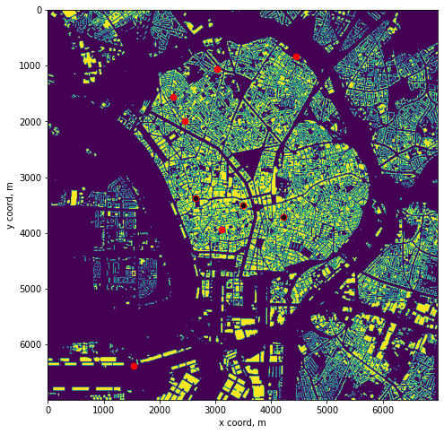
Figure 6: Buildings map and corresponding considered 9 Base Stations positions (in red) for Antwerp dataset

The initial dataset with information about each BS or gateway (GW), Receiving time of the message (RX time), Spreading Factor, Horizontal Dilution of Precision, Latitude, Longitude looks as following:

Dataset preprocessing and analysis.

As an example, in this part we will explain the way the dataset was processed for the future application. We aggregated the received power into cells of the size 10 meters $\times$ 10 meters ($10m\times 10m$) and then averaged this power and translated into signal strength. To perform this aggregation, we measured the distance from the base station location based on local East, North, Up coordinates.

To compute the measurements density after data aggregation into cells of size $10m\times 10m$, we considered the close zone around the base station location of the size $3680m\times 3680m$. As an example, in the following Table 5.2 there is an information about the first three considered base stations from this dataset.

Base station number	Amount of measurements
	Spatial density (per $km^{2}$)
$BS^{\prime}_{1}$	6450	440
$BS^{\prime}_{2}$	5969	389
$BS^{\prime}_{3}$	7118	525

Table 1: Amount of measurements for each base station located in the center of $368\times 368$ image size after $10m\times 10m$ aggregation, Antwerp dataset. Base stations with the highest amount of measurement points around the base station location were selected.

We consider the zone of full city of the size $7000m\times 7000m$ which covers the positions and most of the collected measurements in the city area. We analogically did the $10m\times 10m$ aggregation.

In the initial dataset if in the visited point on the map there was no captured signal, this point for corresponding base station was marked as -200 dBm, so in the Figure 7 the informative range of the signal values lies in [-120; -60] dBm, where the left boundary correspond to the sensitivity of the device.

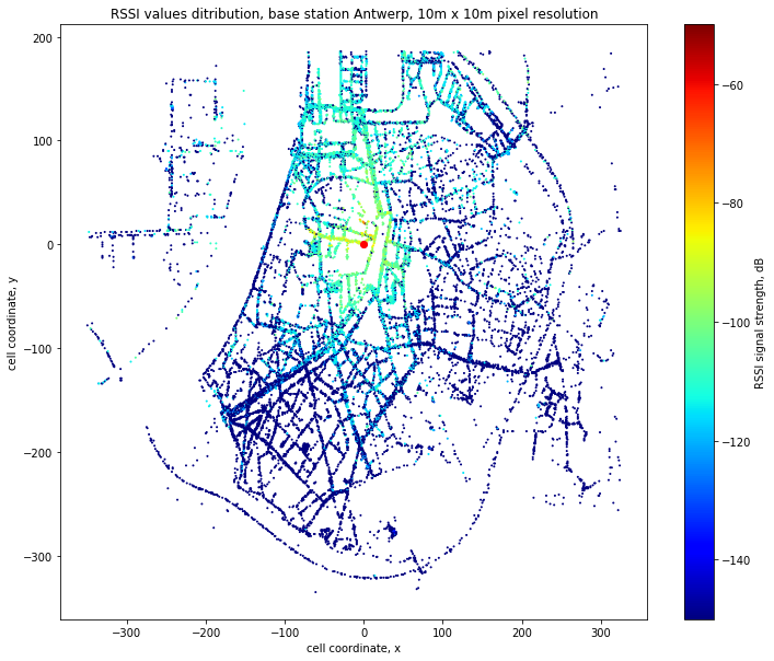
Figure 7: 10x10 $m^{2}$ aggregation for one of the base stations, Antwerp

5.3 Grenoble dataset

Measurement campaign and experimental settings.

There was conducted (and still in progress of extension of number of measurements) an experimental campaign of collecting a LoRa measurements in the real urban environment of Grenoble city. This data is valuable for the future applications especially because of limited amount of available data for the research purposes. The dataset is in process of enlargement (with the installation of new base stations, extension of amount of collected measurements, etc.).

The data is collected for several base stations installed in Grenoble and consists of several parameters such as latitude, longitude, and corresponding RSSI value for each recognized base station. The collected data is similar to one described for Antwerp, but has a bit different structure, see Table 2.

The data was collected by different types of movements: walking of pedestrians, riding a bike or driving a car. Total amount of stored lines in the database collected from 13-01-2021 to 11-01-2022 is 1574588. The data was collected in the frequency band of 868 MHz in the LoRaWAN network by several users with personal tags. One example of stored data is shown in Table 2.

$GateWay\_ID$	$Device\_ID$	$RSS$	$latitude$	$longitude$	$time$
7276ff002e0701e5	70b3d5499b4922dc	-95	45.199308	5.712627	2021-08-29T13:46:35
7276ff002e0701f1	70b3d5499b4922dc	-103	45.199308	5.712627	2021-08-29T13:46:35
…	…	…	…	…	…

Table 2: Example of the dataset format for the field measurements collected in the Grenoble area, where for each connected gateway-tag pair, we report the corresponding device position, time of collection, RSSI value.

To collect the data, COTS telecom grade gateways iBTS from Kerlink manufacturer (see Figure 8) based on the LoRaWAN technology have been used. These gateways have fine time-stamping capability, and are synchronized with the GPS time through a Pulse-per-Second signal generated by GNSS receiver included in the gateway with an accuracy of a few nanoseconds. In LoRaWAN technology, each of the tag uplift packets can be received by more that one base station, depending on the local structure (which cause interference) and mainly path loss. To store the received information from the gateways the LoRaWAN Network Server was used, as it is shown in Table 2 (the amount of stored metrics is bigger – like Signal-to-Noise Ratio, Time of Arrival, uplink network parameters : frequency, DataRate, etc. but here we will focus on the data used in our study).

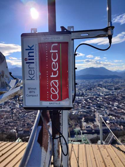
Figure 8: Gateway $BS_{3}$ which is installed on the roof near the cable car station at Bastille, Grenoble

During the data collection, there was different deployment characteristics of the base stations and different amount of them. We consider the second version of the dataset (Grenoble-2) consisted of four base stations located in Grenoble and one which was far from the city region and thus was discarded because of the flatten signal in the zone with the biggest amount of measurements (the first one could be found in [37]). This version will be used in the validation of the results in the experiments section of the Section 6. Position of four considered base stations are shown in the Figure 13(b). This deployment is also interesting as one of the base stations ($BS_{3}$) is installed on the mountain peak higher than all the other base stations and thus quite specific to this database.

Dataset preprocessing and analysis.

First, we needed to filter out of the dataset the unreliable data resulting from errors during the data collection or from measurement artefacts. For example, the exact GPS position could be significantly different from the real position (due to a lack of visibility to satellites) or, due to a specificity in the tag design, data transmission still occur while charging indoor, thus giving both the wrong RSSI value and/or the wrong GPS position. For instance, regarding the latter issue that is quite obvious to detect, we simply rejected all the measurements exhibiting too high RSSI values and/or being static for a long time, which were most likely collected during the charging of the device. Being more precise, first we detected the base stations for which the received signal strength was higher than -55 dBm for the entire acquisition time sequence and then removed the corresponding measurement points collected at the same time for this device with respect to all the other base stations. However, RSSI values saturating at short distances or reaching receiver sensitivity at large distances were preserved in the database, for being somehow indirectly indicative of the tag distance to the BS. Finally, we filtered out all the measurements for which the GPS latitude was not valid (out of tolerated range).

Data aggregation per cell.

Just like for the Antwr¡ep dataset, after removing outliers/artefacts, we then aggregated the signal in the cells. We converted the RSSI into milliWatts (as [dBm] = 10$\log_{10}$[mW]), computed its average per cell in the cells of size $10m\times 10m$, and converted back the result into signal strength values. To perform this aggregation, we measured the distance from the base station $BS_{1}$ location considered to be (0,0) 2D Cartesian coordinate based on local East, North, Up coordinates. Finally, we considered an overall area of interest of $3680m\times 3680m$ (also for the radio mapping application), which covers the entire city, while containing most of the deployed base stations, as shown in the Figure 13(b).

$$\textbf{m}^{BS}=\textbf{P}(\text{{$\eta$}${}^{BS}$})+\epsilon^{BS},$$ (3)

where $\epsilon_{k}^{BS}\sim N(0,({\color[rgb]{0,0,0}\sigma^{BS}})^{2})$ are assumed to be independent and identically distributed residual noise terms (i.i.d.), $d_{0}^{BS}$ is the reference distance, $d_{k}^{BS}=\sqrt{(x^{BS}-x_{k})^{2}+(y^{BS}-y_{k})^{2}}$ is the distance from the base station of 2D Cartesian coordinates ($x^{BS},y^{BS}$) to some tag position ($x_{k},y_{k}$).

To compute the required model parameters, we thus need to solve the set of equations for all the measured points by minimizing the sum of squared errors, as follows:

$$(\textbf{m}^{BS}-\textbf{A}^{BS}\mathbf{\eta}^{BS})^{\intercal}(\textbf{m}^{BS}-\textbf{A}^{BS}\mathbf{\eta}^{BS})\rightarrow\min\limits_{\eta^{BS}}$$ (4)

So the set of optimal parameters is calculated as follows :

$$\hat{\mathbf{\eta}}^{BS}=((\textbf{A}^{BS})^{\intercal}\textbf{A}^{BS})^{-1}(\textbf{A}^{BS})^{\intercal}\textbf{m}^{BS}$$ (5)

Retrospectively and in first approximation, residuals can be interpreted as noise in Equation LABEL:eq:pl_model, so that the standard deviation parameter $\sigma^{BS}$ is simply determined with the optimal model parameters and Equation LABEL:eq:pl_model:

$$\hat{\sigma}^{BS}=std({\color[rgb]{0,0,0}\mathbf{A}^{BS}\hat{\mathbf{\eta}}^{BS}}-\mathbf{m}^{BS})$$ (6)

The results of this LS data fitting process for a few representative Base Stations of the Grenoble dataset are reported in Tables 5 and 6. As it was mentioned above, we compared two settings with or without removing 10% of the cells with the highest variances of measured RSSI values per cell. It was done because of the possible errors or artefacts during the experimental data collection phase (e.g., erroneous GPS position assignment due to satellite visibility conditions) or for a very small amount of collected data that were spotted to have non consistent values (e.g., due to tag failures, etc.). As we can see, removing even such a modest amount of those incriminated pathological cells can significantly impact the computation of the path loss model parameters ruling the deterministic dependency of average RSSI as a function of transmission range, while the standard deviation accounting for the dispersion of RSSI measurements around this average model remains unchanged. By the way, for all the considered Base Stations, the standard deviation value $std$ is observed to be high, which could be imputed to the fact that the underlying average path loss model is too inaccurate and can hardly account for so complex propagation phenomena. Moreover, the amount of points is not so high (maximum around 10% of all the zone of interest), so that data fitting could be degraded by the sparseness and/or non-uniform distribution of the measurement points (with respect to the distance to the base station), which could lead to overweight the influence of some measurements in particular transmission range domains.

BS	$\hat{n}^{BS}$	$\hat{\sigma}^{BS}$, dB	$\hat{P}_{0}^{BS}$, dBm
B2I ($BS_{1}$)	3.20	8.31	-44.58
BCC ($BS_{4}$)	2.32	8.73	-55.21
Bastille ($<$500m) ($BS_{3}$)	2.34	7.87	-67.81
Bastille ($>$1 km) ($BS_{3}$)	2.87	8.07	-33.56
Bastille ($BS_{2}$)	4.01	11.90	-44.74

Table 5: Extracted path loss model parameters for some of the Base stations from Grenoble dataset, as shown on Figure 13(b), with data aggregation in $10m\times 10m$ cells.

BS	$\hat{n}^{BS}$	$\hat{\sigma}^{BS}$, dB	$\hat{P}_{0}^{BS}$, dBm
B2I ($BS_{1}$)	3.46	7.90	-41.77
BCC ($BS_{4}$)	2.59	8.22	-52.18
Bastille ($<$500m) ($BS_{3}$)	2.31	8.01	-68.67
Bastille ($>$1 km) ($BS_{3}$)	2.10	8.62	-51.67
Bastille ($BS_{2}$)	3.65	11.18	-50.49
$BS_{1}\cup BS_{2}\cup BS_{4}$	2.89	10.51	-51.88

Table 6: Recomputed path loss model parameters (after removing 10% of the data) for the same Base stations from Grenoble dataset, as shown on Figure 13(b), with data aggregation in $10m\times 10m$ cells.

In Table 6, there are two sets of parameters for one of the base stations (namely ”Bastille”, $BS_{3}$), as we have identified two distinct zones in terms of topology (and hence, two propagation regimes): (i) on the hill hosting the base station, with a larger angular distribution of the incoming radio signals from the tags and (ii) in the rest of city where the direction of arrival of the signal at the base station does not vary much (and accordingly the receive antenna gain). Moreover, the position of the base station could not cover all the area around, similarly to BS ($BS_{2}$), being located on the Western border/part of the city, this base station naturally serves tags whose transmitted signals arrive systematically from the same side of the city (hence with a reduced span for possible angles of arrivals accordingly, which could somehow bias our extracted statistics). Another remark is that the path loss exponent $n$ can differ significantly from one base station to another and is usually larger in more complex environment contexts (i.e., in case denser buildings are present in the surroundings of the BS), inducing more probable NLoS propagation conditions, and hence stronger shadowing effects even at short distances, which lead to lower RSSI values as a function of the distance in average. But the dispersion around the fitted path loss model, as accounted here by the standard deviation $\sigma$, is also very high on its own, primarily due to a relative lack of accuracy of the single-slope path loss model, but also to the remaining effect of instantaneous received power fluctuations even after in-cell measurements averaging (e.g., caused by multipath under mobility, fast changing tag orientation during measurements collection…).

In Figure 12 below, we also show the overall RSSI distribution over 3 base stations in town (all except the BS “Bastille”, which again experiences a specific propagation regime due to the terrain elevation) as a function of the Tx-Rx distance, along with the superposed fitted function according to the path loss model. As expected, the dispersion accounted by the standard deviation is thus even worse here than that of previous BS-wise parameters extractions, while the other path loss parameters are close to their average values over the three considered base stations.

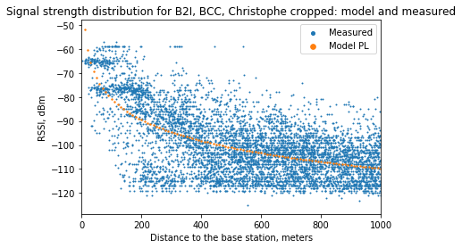
Figure 12: RSSI distribution as a function of transmission range, over 3 base stations: measured values (blue) vs. model-based prediction (orange) with extracted parameters $P_{0}$ = -51.88dBm, $n$=2.89, $\sigma$ = 10.51 dB.

Illustration of RSSI distribution along a LoS street

As an illustration, we consider the longest street in LoS conditions served by the Bastille Base station (Figure 13(a)), where it is theoretically easier to model the behaviour of the signal distribution as a function of transmission range, due to the absence of any big obstacles on the way of the signal. Considering again the path-loss model from Eq. LABEL:eq:pl_model, the parameters have been determined through data fitting and the resulting model is confronted to the measurements, as shown in Figure 14. As we can see, the log-distance classical path-loss model fits fairly well the collected data in terms of average trend, but still with a very large dispersion around the expected/predicted value, indicating also that conventional parametric model-based positioning (i.e., not based on fingerprinting) would be challenging despite the LoS conditions.

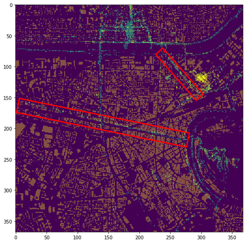
(a) Example of roads in red boxes in LoS with respect to at least one of the deployed BS.

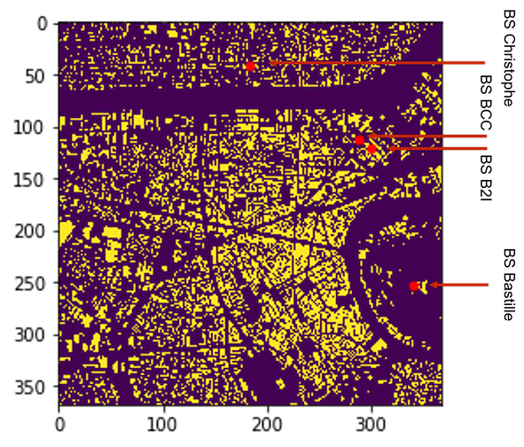
(b) Positions and names of some of the base stations deployed in Grenoble.

Figure 13: Part of the Grenoble map, with a selection of the deployed base station positions (right) and two canonical streets in LoS with respect to the latter.

(a) RSSI measurements distribution and model-based 1D average prediction in LoS, as a function of transmission range

(b) Model-based 2D prediction in LoS, as a function of tag’s position, based on extracted path loss model parameters.

Figure 14: Illustration of RSSI distribution over one particular street: measured RSSI values vs. model-based line-of-sight predictions.

As in this LoS case we can model the signal behaviour, then it is possible to compare the gradients received by this model with the possible interpolations methods and then use it as one of the quality metrics in the map reconstruction problem, the results will be shown in Section 6.

Datasets.

The size of maps are 500 $\times$ 500 pixels for the generated dataset from Paris, 700 $\times$ 700 pixels for the dataset collected in Antwerp and 368 $\times$ 368 for Grenoble. For that, as a reminder, we aggregated and averaged the power of collected measurements in cells/pixels of size 10 meters $\times$ 10 meters by the measured distance from base station location based on local ENU coordinates for Grenoble and Antwerp, while for Paris dataset the cell size is 2 meters $\times$ 2 meters. As we also consider the generalization task, the algorithm should learn from all the available base stations data simultaneously.

In our settings, we only have access to several base stations lacking several orders of magnitude in size compared to aforementioned datasets. To artificially overcome this drawback, we created submatrices of the original images by cutting them into smaller ones (we tested over 96 by 96 pixels size because of memory issues during learning of the neural network for the storing of the model weights). We also added the flipped and mirrored images and we also did a shift in 20 pixels meaning that in our dataset there were overlapping between the images. Moreover, if the amount of pixels with measurements in the initial cutted image was high enough (more than 3% of the presented pixels) then we masked out the randomly sampled rectangle of presented measurements similar to the cutout regularization ([14]). By doing this we force the algorithm to do the reconstructions in the zones without measurements (not only locally) and be more robust to the amount of input data.

Matrices of the side information were used in the models as additional channels concatenated with measurements map. Before feeding the data into the algorithm, all the values have been normalized between 0 and 1 in each channel separately before cutting them into smaller sizes to feed into the models.

Evaluation of the results over held out base stations

To evaluate the result we left one base station out of the initial set of each city to compare further the models performances with baselines, namely test Antwerp and test Grenoble. To do this, all the points were divided into two parts, namely train and test points for 90% and 10% respectively.

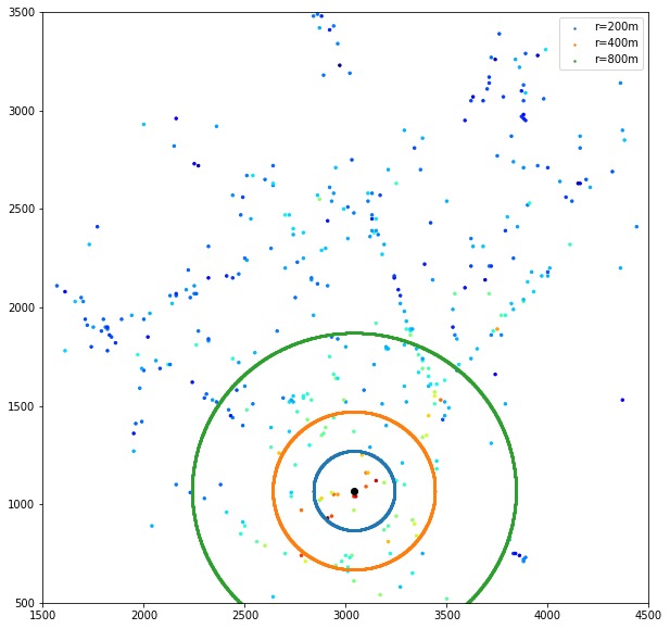
(a) Test points and corresponding circular zones

(b) Train points for the same area for the same base station

Figure 15: Points division for the test base station, Antwerp; Base station location shown as a black point, coordinates are in meters

This will be used throughout all the following sections. Moreover, to highlight the importance of the zones close to base station (as it was mentioned in the Introduction) we compare the performance of the algorithms over different considered circles around the base station location, namely 200 meters, 400 meters and 800 meters radiuses (see Figure 15).

Information about base stations for each city, amount of all points, points, that were used in the validation/test process, and training set are given in Table 7.

We considered state-of-the-art interpolation approaches which are: Total Variation (TV) in-painting by solving the optimization problem, Radial basis functions (RBF) [6] with linear kernel that was found the most efficient, and the $k$ Nearest Neighbours (kNN) regression algorithm. The evolutionary algorithm in the model search phase was implemented using the NAS-DIP [22] package. All experiments were run on NVIDIA GTX 1080 Ti 11GB GPU.

6 Experimental Results

In our experiments, we are primarily interested in addressing the following two questions: $(a)$ does the use of side contextual information aid in the more accurate reconstruction of RSSI maps?; and; $(b)$ to what extent is the search for an optimum NN design effective in the two scenarios considered (Section 4)?

		all points	train points	validation points	status
city	name
Grenoble	$BS_{1}$	6264	5591	673	train
	$BS_{2}$	2728	2448	280	train
	$BS_{3}$	7266	6516	750	train
	$BS_{4}$	6836	6096	740	test
Paris	$BS^{\prime\prime}_{1}$ - $BS^{\prime\prime}_{5}$	250000	7495	242505	train
	$BS^{\prime\prime}_{6}$	250000	7495	242505	test
Antwerp	$BS^{\prime}_{1}$	6060	5440	620	train
	$BS^{\prime}_{2}$	5606	5034	572	train
	$BS^{\prime}_{3}$	7548	6785	763	train
	$BS^{\prime}_{4}$	2539	2276	263	train
	$BS^{\prime}_{5}$	2957	2667	290	train
	$BS^{\prime}_{6}$	4940	4453	487	train
	$BS^{\prime}_{7}$	3154	2829	325	train
	$BS^{\prime}_{8}$	8277	7455	822	train
	$BS^{\prime}_{9}$	4335	3888	447	test

Table 7: Summary over the settings for different cities: total amount of available measurements, points used as an input to the models, validation (test) points that were used also in the computation of the loss (during the evaluation)

Regarding the first point, we consider the following learning settings:

1. given only the measurements (no side information),

2. given both measurements and distance maps,

3. given measurements, distances and elevation maps,

4. given measurements, distances maps and map of amount of buildings on the way from base station to corresponding point in the map (or, in other words, buildings count).

From the standpoint of application, accurate interpolation in all regions where the signal varies the most is critical. We will compare the cumulative mistakes across held-out pixels for each of the zones that are close enough to the test base station for the LoRa signal (by considering the fixed radius of 1 km).

In the following, we will present our findings using the UNet model utilizing side information as a multi-channel input.

6.1 Generalization ability of UNet

We first study the learnability of the UNet model ([49]) for RSSI map reconstruction without the use of unlabeled data. In order to see if there is an effect of using side information we have just considered distance maps as additional context information and considered the model with a hand-crafted classical architecture shown in Figure 16 used for in-painting.

Figure 16: UNet model with hand-crafted architecture proposed for in-painting.

The goal of this early experiment is to validate the usage of UNet for this task and investigate what effects the side information and labeled measurements have. For this we consider the simplest Paris data case where we keep only the points on the roads (as the points could be collected over the street by the vehicle drivers or pedestrians). The difference with Grenoble and Antwrep datasets is in the sampling procedure, as in reality it is very hard to obtain the collected data sampled uniformly in all the regions while in Paris dataset this is the case. All the RSSI measurements also exist in Paris dataset, this allows to see the importance of labeled information in the predictions by varying the percentage of labeled measurements in the training set.

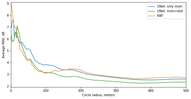
Figure 17: MAE for the distance from the base station for the RBF and fixed UNet outputs over Paris dataset with validation set compliment to the train one, measurements and distances or only measurements input

Figure 17 depicts the evolution of MAE in measurements with respect to the distance to the test base station getting lower in comparison with the RBF interpolation, as well as the overall error becomes smaller ($BS^{\prime\prime}_{6}$ - table 7), of RBF, UNet using only measurements (UNet only msm) and UNet using measurements and distance maps (UNet msm+dist). From these results, it comes that RBF outperforms UNet using only measurements in a circle zone of less than 150 m radius around the base station. However, when distance maps are added to the model’s second channel, the situation is reversed. With the inclusion of side-information, we see that UNet performs around 1 point better in MAE than RBF. This situation is illustrated on the map reconstruction ability of both models around the test base station $BS^{\prime\prime}_{6}$ in Figure 18. As can be observed, the projected signal levels are more discernible on the roads, which are actually the zones of interest where the signal is sought, as predicted by the UNet model.

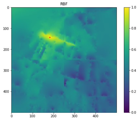
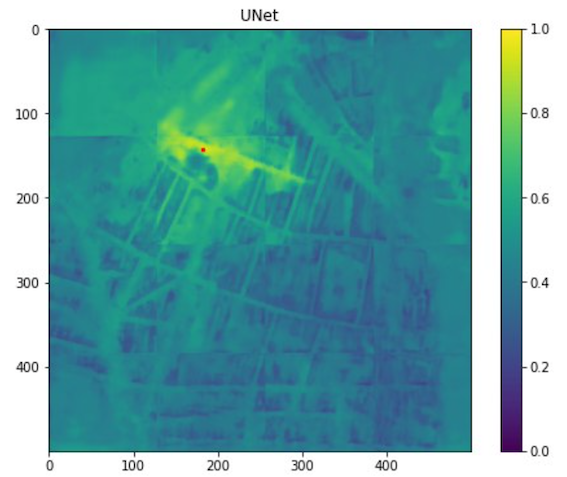
Figure 18: Map reconstruction of RBF (left) and UNet (right) over the test base station $BS^{\prime\prime}_{6}$ in Paris shown by a red dot.

As a result, these findings show that the UNet model can effectively account for side-information. We examined the RBF and UNet models for the influence of labeled measurements on the predictions by altering the percentage of labeled data utilized by RBF for discovering the interpolation and by the UNet model for learning the parameters. With regard to this proportion, Figure 19 displays the average MAE 200 meters (left) and 400 meters (right) away from the test base station. The test error of the RBF model on unseen test data remains constant as the quantity of labeled training data increases, but the test error of the UNet model decreases as this number increases.

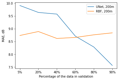
(a) 200 meters from the base station

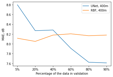
(b) 400 meters from the base station

Figure 19: MAE with respect to different percentage of labeled data in the training set 200 meters (left) and 400 meters (right) away from the test base station.

6.2 The use of unlabeled data by taking into account side information with NAS

Figure 20: Cumulative MAE distribution of $f_{\theta^{\star}_{1}}$ (scenario 1 of Algorithm 1) according to the distance to the test base station for the city of Antwerp $BS^{\prime}_{9}$; with measurements and measurements with distance maps (left) and measurements, distance maps, and building counts or elevation (right).

Model	MAE, dB, 200m	MAE, dB, 400m
RBF[6]	8.34↓	7.04↓
kNN	7.98↓	7.08↓
TV	7.50↓	6.97↓
UNet [49]	6.37↓	6.81↓
DIP [55]	6.55↓	6.63↓
$f_{\theta^{\star}_{1}}$	5.88	6.37

Model	MAE, dB, 200m	MAE, dB, 400m
RBF [6]	4.03↓	5.29↓
kNN	3.84↓	4.92↓
TV	4.53↓	5.91↓
DIP [55]	4.64↓	5.50↓
$f_{\theta^{\star}_{1}}$	3.40	4.32

Table 8: Comparisons between baselines in terms of MAE with respect to the two distances to Antwerp’ test base station $BS^{\prime}_{9}$ (left), and Grenoble test base station $BS_{4}$ (right). Best results are shown in bold.

We now expand our research to real-world data sets from Grenoble and Antwerp, taking into account more side-information and investigating the impact of neural architecture search on the creation of a better NN model. As in this case, the labeled training measurements are scarce we examine the usage of unlabeled data in addition to the labeled measurements as described in the previous section.

We begin by envisaging scenario 1 of Algorithm 1 (Section 4) and investigating the impact of side information on the performance of the optimized NN model discovered by NAS.

Figure 21: Average MAE in dB of all models with respect to the distance to the test base Station $BS^{\prime}_{9}$ for the city of Antwerp.

Figure 20 shows the evolution of MAE inside a circular zone of varied radius for $f_{\theta^{\star}_{1}}$ trained just on measurements and measurements with distance maps (left) and $f_{\theta^{\star}_{1}}$ trained on measurements, distance maps, and building counts or elevation (right) on the test base stations of Antwerp $BS^{\prime}_{9}$. The use of distance maps to supplement measurements improves predictions, which is consistent with our earlier findings. When the third side-information is included, such as height or building counts, we find that the elevation yields better signal estimations than the latter. This is understandable because signal transmission can be severely slowed by building heights.

As a best model obtained by Algorithm 1, scenario 1 we consider the case with three input channels: measurements, distances and elevations and present comparative results with other baselines in Table 8. The lowest errors are shown in boldface. The symbol ^↓ denotes that the error is significantly greater than the best result using the Wilcoxon rank sum test with a p-value threshold of 0.01. According to these findings, $f_{\theta^{\star}_{1}}$ outperforms other state-of-the-art models as well as the UNet model with a handcrafted architecture. These results suggest that the search of an optimal NN model with side-information has strong generalization ability for RSSI map reconstruction.

Figure 21 depicts the average MAE in dB of all models as well as the NN model $f_{\theta^{\star}_{2}}$ corresponding to scenario 2 of Algorithm 1, with respect to the distance to the test base Station $BS^{\prime}_{9}$ for the city of Antwerp. For distances between 200 and 400 meters, $f_{\theta^{\star}_{2}}$ consistently outperforms in terms of MAE. As in paper [37], these findings imply that self-training constitutes a promising future direction for RSSI map reconstruction.

Figure 22 presents the average MAE in dB of all models with respect to the distance to the test base Station $BS_{4}$ for the city of Grenoble. These results are consistent with those obtained over the city of Antwerp.

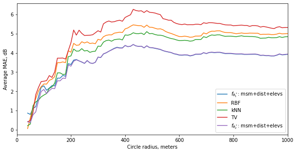
(a) Comparison between different approaches

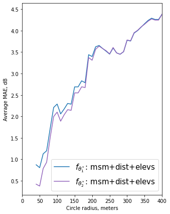
(b) Zoom distance <400m

Figure 22: Average MAE in dB of all models with respect to the distance to the test base Station $BS_{4}$ for the city of Grenoble.

Figure 23: MAE over the distance to the base station evaluated over unseen base stations for Grenoble (left) and Antwerp (right), $f_{\theta^{\star}_{1}}$ is trained over mixed dataset Grenoble+Antwerp.

The general conclusion that we can draw is that knowing about local patterns (even if from different locations/distributions/base stations) allows us to use this information in signal strength map reconstruction for application to unseen measurements from different base stations, demonstrating the ability to generalize output in the same area.

In order to get a finer granularity look at the estimations of the suggested technique, $f_{\theta^{\star}_{2}}$, Figure 24 depicts the errors heatmaps on circular zones of radius 200m and 400m surrounding the test base stations for Antwerp and Grenoble. Each point reflects the difference between the real and predicted signal values. For both cities, we notice that there is

• an overestimation of the signal (higher predicted values than the true ones) within the zone of radius less than 200 meters where the values of the true signal are high. In absolute value, the average MAE in dB are respectively 3.6 for Grenoble and 6.3 for Antwerp.

• an underestimation of the signal (lower predicted values than the true ones) within the zones of radius between 200 and 400 meters where the values of the true signal are low. In absolute value, the average MAE in dB are respectively 4.9 for Grenoble and 6.2 for Antwerp.

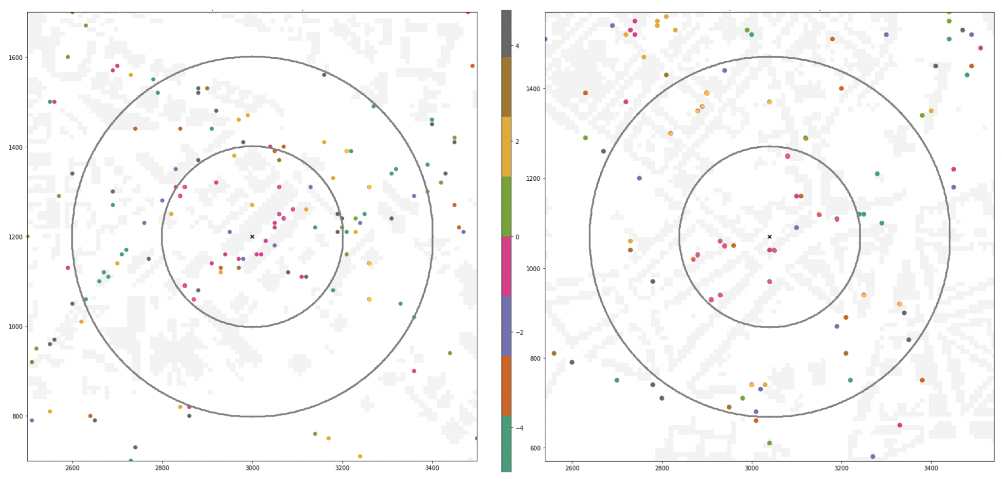
Figure 24: Heatmap of the errors, dB, between true and predicted values of, $f_{\theta^{\star}_{2}}$, over test base stations in Grenoble (left) and Antwerp (right).

To better understand the aforementioned results, we provide the empirical cumulative distribution function of different techniques in a 200-meter zone around the test base stations in Grenoble (Figure 25, left) and Antwerp (Figure 25 right). From these results, it comes that the probabilities of having less absolute dB error is higher for both $f_{\theta^{\star}_{1}}$ and $f_{\theta^{\star}_{2}}$ than the other approaches.

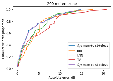
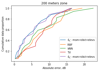
(a)	(b)

Figure 25: Empirical cumulative distribution function of different techniques in a 200-meter zone around the test base stations in Grenoble (left) and Antwerp (right).

The primary takeaway from these findings is that searching a Neural Network model with generalization capabilities might be useful for RSSI map reconstruction. To further investigate in this direction, we considered Scenario 1 of Algorithm 1 in which the training points of both cities are combined, with the goal of evaluating the model’s ability to produce predictions for one of the cities. The average MAE in db with respect to the distance to the base stations for different approaches are shown in Figure 23.

According to these findings, the inclusion of signal data from another city disrupts the search for an efficient NN model and learning its parameters. This is most likely owing to the fact that the data distributions in these cities differ, and it would be interesting to study over alignment strategies, such as those proposed for domain adaptation [27], in order to narrow the gap between these distributions in future work.

7 Conclusion

In this paper we studied the importance of the use of additional side information for the search of an optimized NN architecture for RSSI map reconstruction over three different datasets. We have shown that the addition of distance and elevation of buildings to the measurements allow to significantly reduce the mean absolute error in dB of the obtained NN model with an optimized found architecture. Our proposed approach tends to outperform agnostic techniques especially in the close zone near to the test base stations. We have also shown that our NN based approach has good generalization ability. However, in situations where there exists a distribution shift between two maps, the prediction confidence given by the training model may be highly biased towards, and thus may be not reliable. In reality, a significant difference between two different RSSI maps could lead to complete degradation of the model’s performance due to the large error in pseudo-labels. In practice, approaches like confidence regularization [65] may reduce the number of wrong pseudo-labels, but theoretically, studying the semi-supervised learning under a distribution shift is an important direction for future work.

References

- [1] SARWS c.n. real-time location-aware road weather services composed from multi-modal data. https://www.celticnext.eu/project-sarws/, 2019. Accessed: 26 May 2021.
- [2] M. Aernouts, R. Berkvens, K. Van Vlaenderen, and M. Weyn. Sigfox and lorawan datasets for fingerprint localization in large urban and rural areas. Data, 3(2), 2018.
- [3] Michiel Aernouts. Localization with low power wide area networks. PhD thesis, University of Antwerp, 2022.
- [4] Massih-Reza Amini, Vasilii Feofanov, Loïc Pauletto, Emilie Devijver, and Yury Maximov. Self-training: A survey. CoRR, abs/2202.12040, 2022.
- [5] Sugato Basu, Arindam Banerjee, and Raymond J. Mooney. Semi-supervised clustering by seeding. In Proceedings of the Nineteenth International Conference on Machine Learning, pages 27 – 34, 2002.
- [6] Christopher M. Bishop. Pattern Recognition and Machine Learning (Information Science and Statistics). Springer-Verlag, Berlin, Heidelberg, 2006.
- [7] Geoff Boeing. Osmnx: A python package to work with graph-theoretic openstreetmap street networks. Journal of Open Source Software, 2(12):215, 2017.
- [8] Mathieu Brau, Yoann Corre, and Yves Lostanlen. Assessment of 3d network coverage performance from dense small-cell lte. In 2012 IEEE International Conference on Communications (ICC), pages 6820–6824, 2012.
- [9] Long Cheng, Chengdong Wu, Yunzhou Zhang, Hao Wu, Mengxin Li, and Carsten Maple. A survey of localization in wireless sensor network. International Journal of Distributed Sensor Networks, 2012, 12 2012.
- [10] Wongeun Choi, Yoon-Seop Chang, Yeonuk Jung, and Junkeun Song. Low-power lora signal-based outdoor positioning using fingerprint algorithm. ISPRS International Journal of Geo-Information, 7(11), 2018.
- [11] Ira Cohen, Fabio G. Cozman, Nicu Sebe, Marcelo C. Cirelo, and Thomas S. Huang. Semisupervised learning of classifiers: Theory, algorithms, and their application to human-computer interaction. IEEE Transactions on Pattern Analysis and Machine Intelligence, 26(12):1553–1567, 2004.
- [12] Fabio G. Cozman and Ira Cohen. Unlabeled data can degrade classification performance of generative classifiers. In Fifteenth International Florida Artificial Intelligence Society Conference, pages 327–331, 2002.
- [13] W. Dargie and C. Poellabauer. Fundamentals of Wireless Sensor Networks: Theory and Practice. John Wiley & Sons, 2010.
- [14] Terrance Devries and Graham W. Taylor. Improved regularization of convolutional neural networks with cutout. CoRR, abs/1708.04552, 2017.
- [15] Thomas Elsken, Jan Hendrik Metzen, and Frank Hutter. Neural architecture search: A survey. Journal of Machine Learning Research, 20(55):1–21, 2019.
- [16] A. Enrico and C. Redondi. Radio Map Interpolation Using Graph Signal Processing. IEEE Communications Letters, 22(1):153–156, 2018.
- [17] Omid Esrafilian, Rajeev Gangula, and David Gesbert. Map reconstruction in uav networks via fusion of radio and depth measurements. In ICC 2021 - IEEE International Conference on Communications, pages 1–6, 2021.
- [18] Xiaochen Fan, Xiangjian He, Chaocan Xiang, Deepak Puthal, Liangyi Gong, Priyadarsi Nanda, and Gengfa Fang. Towards system implementation and data analysis for crowdsensing based outdoor RSS maps. IEEE Access, 6:47535–47545, 2018.
- [19] Vasilii Feofanov, Emilie Devijver, and Massih-Reza Amini. Transductive bounds for the multi-class majority vote classifier. In The Thirty-Third AAAI Conference on Artificial Intelligence, pages 3566–3573, 2019.
- [20] X. Han et al. A Two-Phase Transfer Learning-Based Power Spectrum Maps Reconstruction Algorithm for Underlay Cognitive Radio Networks. IEEE Access, 8:81232–81245, 2020.
- [21] Takahiro Hayashi, Tatsuya Nagao, and Satoshi Ito. A study on the variety and size of input data for radio propagation prediction using a deep neural network. In 14th European Conference on Antennas and Propagation, pages 1–5, 2020.
- [22] Kary Ho, Andrew Gilbert, Hailin Jin, and John Collomosse. Neural architecture search for deep image prior, 2020.
- [23] Kazuya Inoue, Koichi Ichige, Tatsuya Nagao, and Takahiro Hayashi. Radio propagation prediction using deep neural network and building occupancy estimation. IEICE Communications Express, advpub, 2020.
- [24] Haifeng Jin, Qingquan Song, and Xia Hu. Auto-keras: An efficient neural architecture search system. In Proceedings of the 25th ACM SIGKDD, pages 1946–1956, 2019.
- [25] Fekher Khelifi, Abbas Bradai, Abderrahim Benslimane, Priyanka Rawat, and Mohamed Atri. A Survey of Localization Systems in Internet of Things. Mobile Networks and Applications, 24(3):761–785, June 2019.
- [26] R. Kubota, S. Tagashira, Y. Arakawa, T. Kitasuka, and A. Fukuda. Efficient survey database construction using location fingerprinting interpolation. In 2013 IEEE 27th International Conference on Advanced Information Networking and Applications (AINA), pages 469–476, 2013.
- [27] Abhishek Kumar, Prasanna Sattigeri, Kahini Wadhawan, Leonid Karlinsky, Rogério Schmidt Feris, Bill Freeman, and Gregory W. Wornell. Co-regularized alignment for unsupervised domain adaptation. pages 9367–9378, 2018.
- [28] M. Laaraiedh, B. Uguen, J. Stephan, Y. Corre, Y. Lostanlen, M. Raspopoulos, and S. Stavrou. Ray tracing-based radio propagation modeling for indoor localization purposes. In 2012 IEEE 17th International Workshop on Computer Aided Modeling and Design of Communication Links and Networks (CAMAD), pages 276–280, 2012.
- [29] R. Levie, Ç. Yapar, G. Kutyniok, and G. Caire. Pathloss prediction using deep learning with applications to cellular optimization and efficient d2d link scheduling. In ICASSP, pages 8678–8682, 2020.
- [30] Jin Li and Andrew D.Heap. A review of comparative studies of spatial interpolation methods in environmental sciences: Performance and impact factors. Ecological Informatics, 6(3):228 – 241, 2011.
- [31] Y. Li, L. Song, Y. Chen, Z. Li, X. Zhang, X. Wang, and J. Sun. Learning dynamic routing for semantic segmentation, 2020.
- [32] Jianxin Liao, Qi Qi, Haifeng Sun, and Jingyu Wang. Radio environment map construction by kriging algorithm based on mobile crowd sensing. Wireless Communications and Mobile Computing, 2019:1–12, 02 2019.
- [33] Yuxiang Lin, Wei Dong, Yi Gao, and Tao Gu. Sateloc: A virtual fingerprinting approach to outdoor lora localization using satellite images. In 2020 19th ACM/IEEE International Conference on Information Processing in Sensor Networks (IPSN), pages 13–24, 2020.
- [34] Chenxi Liu, Liang-Chieh Chen, Florian Schroff, Hartwig Adam, Wei Hua, Alan L Yuille, and Li Fei-Fei. Auto-deeplab: Hierarchical neural architecture search for semantic image segmentation. In Proceedings of CVPR, pages 82–92, 2019.
- [35] Hanxiao Liu, Karen Simonyan, and Yiming Yang. Darts: Differentiable architecture search. arXiv preprint arXiv:1806.09055, 2018.
- [36] Aleksandra Malkova, Massih-Reza Amini, Benoit Denis, and Christophe Villien. Radio map reconstruction with deep neural networks in a weakly labeled learning context with use of heterogeneous side information. In 4th International Conference on Advances in Signal Processing and Artificial Intelligence, 2022.
- [37] Aleksandra Malkova, Loïc Pauletto, Christophe Villien, Benoît Denis, and Massih-Reza Amini. Self-learning for received signal strength map reconstruction with neural architecture search. Lecture Notes in Computer Science, pages 515–526. Springer International Publishing, 2021.
- [38] Yury Maximov, Massih-Reza Amini, and Zaïd Harchaoui. Rademacher complexity bounds for a penalized multi-class semi-supervised algorithm. J. Artif. Intell. Res., 61:761–786, 2018.
- [39] Tatsuya Nagao and Takahiro Hayashi. Study on radio propagation prediction by machine learning using urban structure maps. In 2020 14th European Conference on Antennas and Propagation (EuCAP), pages 1–5, 2020.
- [40] C. Ning and et al. Outdoor location estimation using received signal strength-based fingerprinting. Wireless Pers Commun, 99:365–384, 2016.
- [41] M.A. Oliver and R. Webster. Kriging: a method of interpolation for geographical information systems. International Journal of Geographical Information System, 4(3):313–332, 1990.
- [42] M. J. D. Powell. Radial Basis Functions for Multivariable Interpolation: A Review, page 143–167. USA, 1987.
- [43] Theodore S Rappaport. Wireless communications: Principles and practice. Prentice Hall, 2002.
- [44] M. Raspopoulos and et al. Cross device fingerprint-based positioning using 3D Ray Tracing. In Proc. Computing Conference ( IWCMC’12, pages 147–152, 2012.
- [45] M. Raspopoulos, C. Laoudias, L. Kanaris, A. Kokkinis, C. G. Panayiotou, and S. Stavrou. 3d ray tracing for device-independent fingerprint-based positioning in wlans. In 2012 9th Workshop on Positioning, Navigation and Communication, pages 109–113, 2012.
- [46] E. Real, A. Aggarwal, Y. Huang, and Q. V Le. Regularized evolution for image classifier architecture search. In AAAI, volume 33, pages 4780–4789, 2019.
- [47] A. E. C. Redondi. Radio map interpolation using graph signal processing. IEEE Communications Letters, 22(1):153–156, 2018.
- [48] O. Ronneberger, P.Fischer, and T. Brox. U-net: Convolutional networks for biomedical image segmentation. In Medical Image Computing and Computer-Assisted Intervention (MICCAI), volume 9351 of LNCS, pages 234–241. Springer, 2015.
- [49] Olaf Ronneberger, Philipp Fischer, and Thomas Brox. U-net: Convolutional networks for biomedical image segmentation. In International Conference on Medical image computing and computer-assisted intervention, pages 234–241, 2015.
- [50] V. Rusu and C. Rusu. Radial Basis Functions Versus Geostatistics in Spatial Interpolations. volume 217, 10 2006.
- [51] K. Sato, K. Inage, and T. Fujii. On the performance of neural network residual kriging in radio environment mapping. IEEE Access, 7:94557–94568, 2019.
- [52] Matthias Seeger. Learning with labeled and unlabeled data. Technical report, 2001.
- [53] S. Sorour. and et al. RSS Based Indoor Localization with Limited Deployment Load. In Proc. IEEE Global Communications Conference (GLOBECOM’12), pages 303–308, 2012.
- [54] S. Sorour, Y. Lostanlen, S. Valaee, and K. Majeed. Joint indoor localization and radio map construction with limited deployment load. IEEE Transactions on Mobile Computing, 14(5):1031–1043, 2015.
- [55] Dmitry Ulyanov, Andrea Vedaldi, and Victor Lempitsky. Deep image prior. CoRR, abs/1711.10925, 2017.
- [56] Nicolas Usunier, Massih-Reza Amini, and Cyril Goutte. Multiview semi-supervised learning for ranking multilingual documents. In Machine Learning and Knowledge Discovery in Databases - European Conference, ECML PKDD, pages 443–458, 2011.
- [57] Vladimir Vapnik. Estimation of Dependences Based on Empirical Data: Springer Series in Statistics (Springer Series in Statistics). Springer-Verlag, Berlin, Heidelberg, 1982.
- [58] Vladimir N. Vapnik. Statistical Learning Theory. Wiley-Interscience, 1998.
- [59] Jean-Noël Vittaut, Massih-Reza Amini, and Patrick Gallinari. Learning classification with both labeled and unlabeled data. In Proceedings of the 13th European Conference on Machine Learning (ECML’02), pages 468–476, 2002.
- [60] Kegen Yu, Ian Sharp, and Y. Guo. Ground-Based Wireless Positioning. John Wiley & Sons, Ltd, 06 2009.
- [61] Emmanuel De Bézenac Yuan Yin, Arthur Pajot and Patrick Gallinari. Unsupervised Inpainting for Occluded Sea Surface Temperature Sequences. In Proceedings of the 9th International Workshop on Climate Informatics: CI 2019, Paris, France, 2019.
- [62] Tong Zhang and Frank J. Oles. A probability analysis on the value of unlabeled data for classification problems. In 17th International Conference on Machine Learning, 2000.
- [63] Di Zhu, Ximeng Cheng, Fan Zhang, Xin Yao, Yong Gao, and Yu Liu. Spatial interpolation using conditional generative adversarial neural networks. International Journal of Geographical Information Science, 34(4):735–758, 2020.
- [64] Barret Zoph and Quoc V Le. Neural architecture search with reinforcement learning. arXiv preprint arXiv:1611.01578, 2016.
- [65] Y. Zou, Z. Yu, X. Liu, B. Kumar, and J. Wang. Confidence regularized self-training. In International Conference on Computer Vision - ICCV, pages 5982–5991, 2019.