Safe Collaborative Filtering

Abstract

Excellent tail performance is crucial for modern machine learning tasks, such as algorithmic fairness, class imbalance, and risk-sensitive decision making, as it ensures the effective handling of challenging samples within a dataset. Tail performance is also a vital determinant of success for personalised recommender systems to reduce the risk of losing users with low satisfaction. This study introduces a “safe” collaborative filtering method that prioritises recommendation quality for less-satisfied users rather than focusing on the average performance. Our approach minimises the conditional value at risk (CVaR), which represents the average risk over the tails of users’ loss. To overcome computational challenges for web-scale recommender systems, we develop a robust yet practical algorithm that extends the most scalable method, implicit alternating least squares (iALS). Empirical evaluation on real-world datasets demonstrates the excellent tail performance of our approach while maintaining competitive computational efficiency.

1 Introduction

Owing to the widespread implementation of collaborative filtering (CF) techniques [Hu et al., 2008; Koren et al., 2009; Steck, 2019a; Rendle et al., 2022], recommender systems have become ubiquitous in web applications and are increasingly impacting business profits. The quality of personalisation is critical, particularly for users with low satisfaction, as they are essential for driving user growth, yet their disengagement poses a serious risk to the survival of the business. This is where the problem lies with conventional methods, which focus on optimising performance in terms of averages based on empirical risk minimisation (ERM), with no regard given to harmful errors for tail users. In this paper, we address this problem by utilising a risk measure, conditional value at risk (CVaR) [Rockafellar and Uryasev, 2000, 2002; Pflug, 2000], which represents the average risk for tail users.

Thus far, significant research efforts have been devoted to the computational aspects of risk-averse optimisation [Alexander et al., 2006; Xu and Zhang, 2009; Ahmadi-Javid, 2012]. We are also interested in the scalability of CVaR minimisation for web-scale recommender systems, which must meet strict computational requirements. The challenge of risk-averse CF is scalability in two dimensions: users and items. In the context of personalised ranking, the focus has been on the scalability for the items to be ranked. Numerous studies [Weimer et al., 2007, 2008b, 2008a; Rendle et al., 2009] have addressed the intractability of direct ranking optimisation through the “score-and-sort” approach, where, given a user, a method predicts scores for all items and then sorts them according to their scores. To attain further scalability for a large item catalogue, practical methods adopt pointwise loss functions, enabling parallel model training for users and items [Hu et al., 2008; He et al., 2016; Bayer et al., 2017]. The key to these efficient methods is the separability of pointwise objectives, which allows efficient block coordinate algorithms, such as alternating least squares (ALS) [Hu et al., 2008]. However, integrating CVaR optimisation into this approach faces a severe obstacle because of the non-smooth and non-linear functions in CVaR (i.e. check functions), which hinder the separability and parallel computation for items.

Our contribution in this paper is to devise a practical algorithm for risk-averse CF by eliminating the mismatch between CVaR minimisation and personalised ranking. The paper is structured as follows. In Section 2, we show that applying CVaR minimisation to matrix factorisation (MF) is computationally expensive. This is mainly due to the non-linear and non-smooth check function $\max(0,\cdot)$ even with a block multi-convex, separable loss. In Section 3, we overcome this challenge by using a smoothing technique of quantile regression [Fernandes et al., 2021; He et al., 2021; Tan et al., 2022] and establish a block coordinate solver that is embarrassingly parallelisable for both users and items. The related work is discussed in Section 4, and our experiments are described in Section 5.

2 Setting and Challenge

Following conventional studies (e.g. [Weimer et al., 2007, 2008b, 2008a]), we view collaborative filtering as a ranking problem. In this setting, we have access to the set $\mathcal{S}$ of implicit feedback $(i,j)$ indicating that user $i$ has preferred item $j$. We denote the sets of users and items observed in $\mathcal{S}$ as $\mathcal{U}$ and $\mathcal{V}$, respectively. For convenience, we also define $\mathcal{V}_{i}$ to be the set of items preferred by user $i$, i.e. $\mathcal{V}_{i}\coloneqq\{j\in\mathcal{V}\mid(i,j)\in\mathcal{S}\}$, and $\mathcal{U}_{j}$ to be the set of users that have selected item $j$, i.e. $\mathcal{U}_{j}\coloneqq\{i\in\mathcal{U}\mid(i,j)\in\mathcal{S}\}$. The aim of this problem is to learn a scoring function $\bm{f}_{\theta}$ parametrised by $\theta$, which produces a structured prediction $\bm{f}_{\theta}(i)\in\mathbb{R}^{|\mathcal{V}|}$ having the same order of underlying $i$’s preferences on $\mathcal{V}$; we may denote the predicted score for $(i,j)$ by $f_{\theta}(i,j)$.

Pairwise ranking optimisation.

Conventional studies [Rendle et al., 2009; Lee et al., 2014; Park et al., 2015] often formulate this problem as pairwise ranking optimisation within the ERM framework, aiming to minimise a population risk $\min_{\theta}\mathbb{E}_{(i,\mathcal{V}_{i})}\left[\ell_{\mathrm{pair}}(\bm{f}_{\theta}(i),\mathcal{V}_{i})\right]$, where $\mathbb{E}_{(i,\mathcal{V}_{i})}$ represents the expectation over user $i$ with feedback $\mathcal{V}_{i}$. Here, the loss function $\ell_{\mathrm{pair}}$ is expressed as follows:

$$\ell_{\mathrm{pair}}(\bm{f}_{\theta}(i),\mathcal{V}_{i})\coloneqq\frac{1}{|\mathcal{V}_{i}|}\sum_{j\in\mathcal{V}_{i}}\sum_{j^{\prime}\in\mathcal{V}}\mathds{1}\{f_{\theta}(i,j^{\prime})\geq f_{\theta}(i,j)\},$$ (Pairwise Loss)

where $\mathds{1}\{\cdot\}$ is the indicator function. Because this loss function is piece-wise constant and intractable, its convex upper bounds are utilised, such as margin hinge loss [Weimer et al., 2008b] and softplus loss [Rendle et al., 2009]. However, such loss functions lead to non-separability for items; that is, a loss cannot be decomposed into the sum of independent functions $\{g_{j}\}_{j\in\mathcal{V}}$ for items: $\ell_{\mathrm{pair}}(\bm{f}_{\theta}(i),\mathcal{V}_{i})\neq\sum_{j\in\mathcal{V}}g_{j}(f_{\theta}(i,j))$. Thus, this approach often relies on gradient-based optimisers, but such optimisers suffer from slow convergence [Rendle and Freudenthaler, 2014].

Convex and separable upper bound.

To address this non-separability issue, conventional methods utilise convex and separable loss functions (i.e. pointwise loss [Hu et al., 2008; Zhou et al., 2008]). We also adopt the following convex and separable upper bound of Eq. Pairwise Loss,

$$\frac{1}{|\mathcal{V}_{i}|}\sum_{j\in\mathcal{V}_{i}}\left[1-f_{\theta}(i,j)\right]^{2}+\beta_{0}\cdot\sum_{j\in\mathcal{V}}f_{\theta}(i,j)^{2},$$ (1)

where $\beta_{0}\geq 1/|\mathcal{V}|$ is a hyperparameter. The derivation is deferred to Appendix A.

We here implement the model of $\bm{f}_{\theta}$ using matrix factorisation (MF), which is a popular model owing to its scalability [Hu et al., 2008; Koren et al., 2009; Rendle et al., 2022]. The model parameters of an MF comprise two blocks, i.e. $\theta=(\mathbf{U},\mathbf{V})$ where $\mathbf{U}\in\mathbb{R}^{|\mathcal{U}|\times d}$ and $\mathbf{V}\in\mathbb{R}^{|\mathcal{V}|\times d}$ are the embedding matrices of users and items, respectively. The prediction for user $i$ is then defined by $\bm{f}_{\theta}(i)=\mathbf{V}\mathbf{u}_{i}$, where $\mathbf{u}_{i}\in\mathbb{R}^{d}$ represents the $i$-th row of $\mathbf{U}$, and the ERM objective can be expressed as follows:

$$\min_{\mathbf{U},\mathbf{V}}\frac{1}{|\mathcal{U}|}\sum_{i\in\mathcal{U}}\ell(\mathbf{V}\mathbf{u}_{i},\mathcal{V}_{i})+\Omega(\mathbf{U},\mathbf{V}),$$ (ERM-MF)

where

$$\ell(\mathbf{V}\mathbf{u}_{i},\mathcal{V}_{i})\coloneqq\frac{1}{|\mathcal{V}_{i}|}\sum_{j\in\mathcal{V}_{i}}\frac{1}{2}(1-\mathbf{u}_{i}^{\top}\mathbf{v}_{j})^{2}+\frac{\beta_{0}}{2}\|\mathbf{V}\mathbf{u}_{i}\|_{2}^{2}.$$ (Implicit MF)

Here, $\Omega(\mathbf{U},\mathbf{V})=\tfrac{1}{2}\|\mathbf{\Lambda}_{u}^{1/2}\mathbf{U}\|_{F}^{2}+\tfrac{1}{2}\|\mathbf{\Lambda}_{v}^{1/2}\mathbf{V}\|_{F}^{2}$ denotes L2 regularisation, with diagonal matrices $\mathbf{\Lambda}_{u}\in\mathbb{R}^{|\mathcal{U}|\times|\mathcal{U}|}$ and $\mathbf{\Lambda}_{v}\in\mathbb{R}^{|\mathcal{V}|\times|\mathcal{V}|}$ representing user- and item-dependent Tikhonov weights. Because a pointwise loss enables a highly scalable ALS algorithm owing to separability, it is widely used for scalable methods, such as implicit alternating least squares (iALS) [Hu et al., 2008]. In fact, iALS is implemented in practical applications [Meng et al., 2016] and is still known as one of the state-of-the-art methods [Rendle et al., 2022]. The only difference between our loss and iALS loss is the normalisation factor $1/|\mathcal{V}_{i}|$ in the first term. For further details, see Appendix B.

Figure 1: Illustration of CVaR

Conditional value at risk (CVaR).

In contrast to ERM, which corresponds to the average case, we focus on a more pessimistic scenario. Specifically, the objective of $(1-\alpha)$-CVaR minimisation involves a conditional expectation,

$$\min_{\theta}\mathbb{E}_{(i,\mathcal{V}_{i})}\left[\ell(\bm{f}_{\theta}(i),\mathcal{V}_{i})\mid\ell(\bm{f}_{\theta}(i),\mathcal{V}_{i})\geq\ell_{1-\alpha}\right],$$ (2)

where $\ell_{1-\alpha}$ is the $(1-\alpha)$-quantile of the loss distribution, called value at risk (VaR) [Jorion, 2007]. Since this is difficult to optimise, Rockafellar and Uryasev [2000, 2002] proposed the following reformulation:

$$\min_{\theta,\xi}\left\{\xi+\alpha^{-1}\mathbb{E}_{(i,\mathcal{V}_{i})\sim\mathds{P}}[\max(0,\ell(\bm{f}_{\theta}(i),\mathcal{V}_{i})-\xi)]\right\}.$$ (3)

This objective is rather easy to optimise, as it is block multi-convex w.r.t. both $\xi$ and $\theta$ when the loss function is convex w.r.t. $\theta$.

CVaR-MF.

Now, we apply the above CVaR formulation to Eq. ERM-MF as follows:

$$\min_{\mathbf{U},\mathbf{V},\xi}\left\{\xi+\frac{1}{\alpha|\mathcal{U}|}\sum_{i\in\mathcal{U}}\max(0,\ell(\mathbf{V}\mathbf{u}_{i},\mathcal{V}_{i})-\xi)+\Omega(\mathbf{U},\mathbf{V})\right\}.$$ (CVaR-MF)

However, optimising this objective is still challenging. Although subgradient methods [Rockafellar and Uryasev, 2000] enable parallel optimisation of non-smooth objectives without requiring separability, such gradient-based solvers are known to be impractical in the context of large-scale recommender systems. On the other hand, the obstacle in designing an efficient algorithm lies in the non-linearity of the ramp function $\rho_{1}(x)=\max(0,x)$. It destroys the objective’s separability for items, making it impossible to solve the subproblem for each row of $\mathbf{V}$ in parallel, even with the separable upper bound in Eq. Implicit MF.

3 SAFER₂: Smoothing Approach for Efficient Risk-averse Recommender

Figure 2: Convolution-type smoothing.

3.1 Convolution-type smoothing for CVaR

To overcome the non-smoothness of CVaR, we utilise a smoothing technique for quantile regression [Fernandes et al., 2021; He et al., 2021; Tan et al., 2022; Man et al., 2022], which involves the integral convolution with smooth functions, called mollifiers as studied by Schwartz [1951]; Friedrichs [1944]; Sobolev [1938] among others. We introduce the notation $k_{h}(\cdot)\coloneqq h^{-1}k(\cdot/h)$, where $k(\cdot)$ is a kernel density function satisfying $\int k(u)du=1$ and $h>0$ denotes bandwidth, while $K_{h}$ represents its CDF; $K_{h}(u)\coloneqq\int_{-\infty}^{u}k_{h}(v)dv$. We then define a smoothed check function $\rho_{1-\alpha}\ast k_{h}\colon\mathbb{R}\to\mathbb{R}$ as follows:

$$(\rho_{1-\alpha}\ast k_{h})(u)\coloneqq\int\rho_{1-\alpha}(v)k_{h}(v-u)dv,$$ (4)

where $*$ is called the convolution operator. The resulting function $\rho_{1-\alpha}\ast k_{h}$ attains strict convexity when $k_{h}$ is strictly convex. We then obtain the objective of convolution-type smoothed CVaR:

$$\min_{\mathbf{U},\mathbf{V},\xi} \Bigl{\{}\underbrace{\xi+\frac{1}{\alpha|\mathcal{U}|}\sum_{i\in\mathcal{U}}(\rho_{1}\ast k_{h})(\ell(\mathbf{V}\mathbf{u}_{i},\mathcal{V}_{i})-\xi)}_{\Psi_{1-\alpha}(\mathbf{U},\mathbf{V},\xi)}+\Omega(\mathbf{U},\mathbf{V})\Bigr{\}}.$$ (CtS-CVaR-MF)

We hereafter denote the functional $\Psi_{1-\alpha}(\mathbf{U},\mathbf{V},\xi)$ as $(1-\alpha)$-CtS-CVaR. If $\ell$ is block multi-convex w.r.t. $\mathbf{U}$ and $\mathbf{V}$, then $\Psi_{1-\alpha}(\mathbf{U},\mathbf{V},\xi)$ is also block multi-convex w.r.t. $\mathbf{U}$, $\mathbf{V}$, and $\xi$ because $(\rho_{1}\ast k_{h})$ is convex and non-decreasing. Therefore, we consider a block coordinate algorithm, where we cyclically update each block while fixing the other blocks to the current estimates. That is,

$$\xi^{(t+1)} =\operatorname*{argmin}_{\xi}\Psi_{1-\alpha}(\mathbf{U}^{(t)},\mathbf{V}^{(t)},\xi),$$ (5)

$$(\mathbf{U}^{(t+1)},\mathbf{V}^{(t+1)}) =\operatorname*{argmin}_{\mathbf{U},\mathbf{V}}\Psi_{1-\alpha}(\mathbf{U},\mathbf{V},\xi^{(t+1)}).$$ (6)

Because the subproblems lack a closed-form update and block separability, we develop our proposed method, Smoothing Approach For Efficient Risk-averse Recommender (SAFER₂), which exploits the objective’s smoothness to yield block multi-convex and separable optimisation. In the following, we present the overall algorithm of SAFER₂, and Appendix D contains the detailed implementation.

3.2 Convolution-type smoothed quantile estimation

The smoothed $(\rho_{1-\alpha}\ast k_{h})$ is twice differentiable, so a natural approach to finding the solution $\xi^{*}$ is to use the Newton–Raphson (NR) algorithm. At iteration $l<L$ in the $(k+1)$-th update, it estimates $\xi$ as follows:

$$\xi_{l+1}^{(t+1)}=\xi_{l}^{(t+1)}-\gamma_{l}\cdot d_{l}^{(t+1)},\quad\text{where~{}}d_{l}^{(t+1)}\coloneqq\frac{\nabla_{\xi}\Psi_{1-\alpha}(\mathbf{U}^{(t)},\mathbf{V}^{(t)},\xi_{l}^{(t+1)})}{\nabla_{\xi}^{2}\Psi_{1-\alpha}(\mathbf{U}^{(t)},\mathbf{V}^{(t)},\xi_{l}^{(t+1)})},$$ (7)

where $\gamma_{l}>0$ represents the step size. The convolution-type smoothing was originally used with check functions for quantile regression, and we are the first to apply it to smooth the CVaR objective. Interestingly, even if we apply the convolution-type smoothing to $\max(0,\cdot)$ in CVaR, optimising $\xi$ for a given $\mathbf{U}$ and $\mathbf{V}$ is equivalent to a smoothed (unconditional) quantile estimation; the proof is deferred to Section C.3.

Efficient loss computation.

The naïve computation of $\ell(\mathbf{V}\mathbf{u}_{i},\mathcal{V}_{i})$ for every user is infeasible in large-scale settings owing to the score penalty $\|\mathbf{V}\mathbf{u}_{i}\|_{2}^{2}$, which implies the materialisation of the recovered matrix $\mathbf{U}\mathbf{V}^{\top}$ with the cost of $\mathcal{O}(|\mathcal{U}||\mathcal{V}|d^{2})$. We can reduce this cost by pre-computing and caching the Gramian matrix $\mathbf{V}^{\top}\mathbf{V}\in\mathbb{R}^{d\times d}$ in $\mathcal{O}(|\mathcal{V}|d^{2})$ and computing the loss of user $i$ with $\|\mathbf{V}\mathbf{u}_{i}\|_{2}^{2}=\mathbf{u}_{i}^{\top}(\mathbf{V}^{\top}\mathbf{V})\mathbf{u}_{i}$ in $\mathcal{O}(d^{2})$, thus leading to the overall cost of $\mathcal{O}((|\mathcal{U}|+|\mathcal{V}|)d^{2})$.

Stochastic optimisation for many users.

Estimating $\xi$ can be expensive because of the $\mathcal{O}(|\mathcal{U}|)$ computational cost for each NR step, particularly for many users. We can alleviate this extra cost by using stochastic algorithms [Xu et al., 2016; Roosta-Khorasani and Mahoney, 2019], in which we randomly sample the user subset $\mathcal{U}_{b}\subset\mathcal{U}$ and then estimate the direction by a sample average approximation $\widehat{\Psi}_{1-\alpha}(\mathbf{U},\mathbf{V},\xi)\coloneqq\xi+(\alpha|\mathcal{U}_{b}|)^{-1}\sum_{i\in\mathcal{U}_{b}}(\rho_{1}\ast k_{h})(\ell(\mathbf{V}\mathbf{u}_{i},\mathcal{V}_{i})-\xi)$. This also allows us to use a backtracking line search [Armijo, 1966] to determine an appropriate step size $\gamma_{t}$ while keeping computational costs in $\mathcal{O}(|\mathcal{U}_{b}|L)$ where $L>0$ is the number of NR iterations.

3.3 Primal-dual splitting for parallel computation

The major obstacle to the scalability for items is the row-wise coupling of $\mathbf{V}$ stemming from non-linear composite $(\rho_{1}\ast k_{h})(\ell(\mathbf{V}\mathbf{u}_{i},\mathcal{V}_{i}))$. Because $(\rho_{1}\ast k_{h})$ is closed and convex, we can express it as its biconjugate $(\rho_{1}\ast k_{h})(r)=\max_{z}\left\{z\cdot r-(\rho_{1}\ast k_{h})^{*}(z)\right\}$. This allows us to reformulate the original subproblem of $\mathbf{U}$ and $\mathbf{V}$ as the following saddle-point optimisation:

$$\min_{\mathbf{U},\mathbf{V}}\max_{\mathbf{z}}\left\{\xi+\frac{1}{\alpha|\mathcal{U}|}\sum_{i\in\mathcal{U}}[z_{i}\cdot(\ell(\mathbf{V}\mathbf{u}_{i},\mathcal{V}_{i})-\xi)-(\rho_{1}\ast k_{h})^{*}\left(z_{i}\right)]+\Omega(\mathbf{U},\mathbf{V})\right\},$$ (PD-Splitting)

where $\mathbf{z}\in\mathbb{R}^{|\mathcal{U}|}$ represents the vector of dual variables. Our algorithm alternatingly updates each block of variables (i.e. $\mathbf{z}$, $\mathbf{U}$ and $\mathbf{V}$) by solving its subproblem. As we will discuss below, owing to convolution-type smoothing, the inner maximisation for the dual variable $\mathbf{z}$ can be solved exactly and efficiently, and thus our algorithm operates similarly to a block coordinate descent [Tseng, 2001] for the primal variables $\mathbf{U}$ and $\mathbf{V}$. Through numerical experiments, we will show this algorithm converges in practice when given a sufficiently large bandwidth $h$.

Dual-free optimisation.

In the $\mathbf{z}$ step, we solve the problem for the dual variable $z_{i}$ of each user $i$,

$$z_{i}^{(t+1)}=\operatorname*{argmax}_{z_{i}}\left\{z_{i}\cdot(\ell(\mathbf{V}^{(t)}\mathbf{u}_{i}^{(t)},\mathcal{V}_{i})-\xi^{(t+1)})-(\rho_{1}\ast k_{h})^{*}(z_{i})\right\},$$ (8)

where the convex conjugate $(\rho_{1}\ast k_{h})^{*}$ does not necessarily have a closed-form expression. Fortunately, with convolution-type smoothing, we can sidestep this issue and solve each subproblem without explicitly computing $(\rho_{1}\ast k_{h})^{*}$. Let $r_{i}^{(t)}\coloneqq\ell(\mathbf{V}^{(t)}\mathbf{u}_{i}^{(t)},\mathcal{V}_{i})-\xi^{(t+1)}$ denote the residual for user $i\in\mathcal{U}$, then the first-order optimality condition for $z_{i}$ is:

$$r_{i}^{(t)}-\nabla_{z_{i}}(\rho_{1}\ast k_{h})^{*}(z_{i}^{(t+1)})=0.$$

Exploiting the property of convex conjugate, we can obtain the gradient $\nabla_{z_{i}}(\rho_{1}\ast k_{h})^{*}(z_{i}^{(t+1)})$ by

$$\nabla_{z_{i}}(\rho_{1}\ast k_{h})^{*}(z_{i})=\operatorname*{argmin}_{x}\left\{-x\cdot z_{i}+(\rho_{1}\ast k_{h})(x)\right\}\Longleftrightarrow -z_{i}^{(t+1)}+1-K_{h}(-x^{\ast})=0$$

$$\Longleftrightarrow x^{\ast}=-K_{h}^{-1}(1-z_{i}^{(t+1)}).$$

Recall that $K_{h}$ is the CDF of $k_{h}$ and has its inverse $K_{h}^{-1}$ (i.e. the quantile function). Consequently, we obtain the closed-form solution of $z_{i}^{(t+1)}$ as:

$$r_{i}^{(t)}-\nabla_{\mathbf{z}}(\rho_{1}\ast k_{h})^{*}(z_{i}^{(t+1)})=0\Longleftrightarrow z_{i}^{(t+1)}=1-K_{h}(-r_{i}^{(t)}).$$

Once we have $\xi^{(t+1)}$, all $z_{i}^{(t+1)}$ can be computed in parallel for users, and $K_{h}$ can also be computed effortlessly when using standard kernels for $k_{h}$, such as Gaussian, sigmoid, and logistic kernels.

Re-weighted alternating least squares.

When given dual variables $\mathbf{z}$, the optimisation problem of $\mathbf{U}$ and $\mathbf{V}$ forms a re-weighted ERM, i.e. $\min_{\mathbf{U},\mathbf{V}}\left\{(\alpha|\mathcal{U}|)^{-1}\sum_{i\in\mathcal{U}}z_{i}\cdot\ell(\mathbf{V}\mathbf{u}_{i},\mathcal{V}_{i})+\Omega(\mathbf{U},\mathbf{V})\right\}$, which is separable and block strongly multi-convex w.r.t. the rows of $\mathbf{U}$ and $\mathbf{V}$. Consequently, this step is efficient to the same extent as the most efficient ALS solver of Hu et al. [2008]. It is also worth noting that, as proposed in Hu et al. [2008], we pre-compute Gramian matrices $\mathbf{V}^{\top}\mathbf{V}$ and $\mathbf{U}^{\top}\text{diagMat}(\mathbf{z})\mathbf{U}$ to reuse them for efficiently compute the separable subproblems in parallel (a.k.a. the Gramian trick [Krichene et al., 2018; Rendle et al., 2022]). It is also possible to parallelise each pre-computation step by considering $\mathbf{V}^{\top}\mathbf{V}=\sum_{j\in\mathcal{V}}\mathbf{v}_{j}\mathbf{v}_{j}^{\top}$ and $\mathbf{U}^{\top}\text{diagMat}(\mathbf{z})\mathbf{U}=\sum_{i\in\mathcal{U}}z_{i}\cdot\mathbf{u}_{i}\mathbf{u}_{i}^{\top}$.

Tikhonov regularisation.

Previous empirical observations show that Tikhonov weight matrices $\mathbf{\Lambda}_{u}$ and $\mathbf{\Lambda}_{v}$ are critical in enhancing the ranking quality of MF [Zhou et al., 2008; Rendle et al., 2022]. Hence, we develop a regularisation strategy for SAFER₂ based on condition numbers, which characterise the numerical stability of ridge-type problems. Let $\lambda_{u}^{(i)}$ and $\lambda_{v}^{(j)}$ denote the $(i,i)$-element of $\mathbf{\Lambda}_{u}$ and the $(j,j)$-element of $\mathbf{\Lambda}_{v}$, respectively. We propose the regularisation weights for user $i$ and $j$ as follows:

$$\lambda_{u}^{(i)}=\frac{\lambda}{\alpha|\mathcal{U}|}\left(1+\beta_{0}|\mathcal{V}|\right),\quad\lambda_{v}^{(j)}=\frac{\lambda}{\alpha|\mathcal{U}|}\Bigl{(}\sum_{i\in\mathcal{U}_{j}}\frac{1}{|\mathcal{V}_{i}|}+\beta_{0}\alpha|\mathcal{U}|\Bigr{)}.$$

Here, $\lambda>0$ represents the base weight that requires tuning. This strategy introduces only one hyperparameter and empirically improves final performance. See Appendix E for a detailed derivation.

3.4 Computational complexity and scalability

The computational cost of the $\xi$ step is $\mathcal{O}(|\mathcal{U}_{b}|L)$, and for the $\mathbf{U}$ and $\mathbf{V}$ steps is $\mathcal{O}(|\mathcal{S}|d^{2}+(|\mathcal{U}|+|\mathcal{V}|)d^{3})$ [Hu et al., 2008]. Therefore, the overall complexity per epoch is $\mathcal{O}(|\mathcal{U}_{b}|L+|\mathcal{S}|d^{2}+(|\mathcal{U}|+|\mathcal{V}|)d^{3})$. The linear dependency on $|\mathcal{U}|$ and $|\mathcal{V}|$ can be alleviated arbitrarily by increasing the parallel degree owing to separability. The cubic dependency on $d$ can be circumvented by leveraging inexact solvers such as the conjugate gradient method [Tan et al., 2016] and subspace-based block coordinate descent [Rendle et al., 2021] to update each row of $\mathbf{U}$ and $\mathbf{V}$. The sketch of the algorithm is shown in Algorithm 1.

1

Input : $\{\mathcal{V}_{i}\}_{i\in\mathcal{U}}$

Output : $\mathbf{U},\mathbf{V}$

2 $(\mathbf{U},\mathbf{V},\xi,\{\ell_{i}\}_{i\in\mathcal{U}},\mathbf{G}_{V})\leftarrow$ Initialise($\{\mathcal{V}_{i}\}_{i\in\mathcal{U}}$)

3 for $t\leftarrow 1$ to $T$ do

4       $\xi\leftarrow$ ComputeXi($\xi,\{\ell_{i}\}_{i\in\mathcal{U}}$)

5       for $i\leftarrow 1$ to $|\mathcal{U}|$ do

6             $z_{i}\leftarrow 1-K_{h}(\xi-\ell_{i})$

7             $\mathbf{u}_{i}\leftarrow\operatorname*{argmin}_{\mathbf{u}}\{\frac{z_{i}}{\alpha|\mathcal{U}|}\ell(\mathbf{V}\mathbf{u},\mathcal{V}_{i})+\frac{\lambda_{u}^{(i)}}{2}\|\mathbf{u}\|_{2}^{2}\}$

8       end for

9      $\widetilde{\mathbf{G}}_{U}\leftarrow\sum_{i\in\mathcal{U}}z_{i}\cdot\mathbf{u}_{i}\mathbf{u}_{i}^{\top}$

10       for $j\leftarrow 1$ to $|\mathcal{V}|$ do

11             $\mathbf{v}_{j}\leftarrow\operatorname*{argmin}_{\mathbf{v}}\{\Psi_{1-\alpha}(\mathbf{U},\mathbf{V},\xi)+\frac{\lambda_{v}^{(j)}}{2}\|\mathbf{v}\|_{2}^{2}\}$

12       end for

13      $\mathbf{G}_{V}\leftarrow\sum_{j\in\mathcal{V}}\mathbf{v}_{j}\mathbf{v}_{j}^{\top}$

14       $\forall i\in\mathcal{U},\,\ell_{i}\leftarrow\ell(\mathbf{V}\mathbf{u}_{i},\mathcal{V}_{i})$

15      

16 end for

return $\mathbf{U},\mathbf{V}$

Algorithm 1 SAFER₂ solver.

1

2Function  Initialise($\{\mathcal{V}_{i}\}_{i\in\mathcal{U}}$):

3       $\forall i\in\mathcal{U},~{}\mathbf{u}_{i}\sim\mathcal{N}(\vec{0},(\sigma/\sqrt{d})\mathbf{I}_{d})$

4       $\forall j\in\mathcal{V},~{}\mathbf{v}_{j}\sim\mathcal{N}(\vec{0},(\sigma/\sqrt{d})\mathbf{I}_{d})$

5       $\mathbf{G}_{V}\leftarrow\sum_{j\in\mathcal{V}}\mathbf{v}_{j}\mathbf{v}_{j}^{\top}$

6       $\forall i\in\mathcal{U},\,\ell_{i}\leftarrow\ell(\mathbf{V}\mathbf{u}_{i},\mathcal{V}_{i})$

7       $\xi\leftarrow(1/|\mathcal{U}|)\sum_{i\in\mathcal{U}}\ell_{i}$

8       return $\mathbf{U},\mathbf{V},\xi,\{\ell_{i}\}_{i\in\mathcal{U}},\mathbf{G}_{V}$

9 end

10Function  ComputeXi($\xi,\{\ell_{i}\}_{i\in\mathcal{U}}$):

11       for $l\leftarrow 1$ to $L$ do

12             Uniformly draw $\mathcal{U}_{b}\subseteq\mathcal{U}$

13             $\widehat{d}\leftarrow\frac{\nabla_{\xi}\widehat{\Psi}_{1-\alpha}(\xi)}{\nabla_{\xi}^{2}\widehat{\Psi}_{1-\alpha}(\xi)}$

14             Backtracking line search of $\gamma$,

15             $\xi\leftarrow\xi-\gamma\cdot\widehat{d}$

16       end for

17      return $\xi$

18 end

Algorithm 2 Subroutines for SAFER₂.

4 Related work

Risk-averse optimisation.

Coherent risk measures such as CVaR (also called expected shortfall [Acerbi and Tasche, 2002]) are widely used instead of (incoherent) VaR [Artzner, 1997; Artzner et al., 1999; Jorion, 2007]. Despite the desirable properties of CVaR [Pflug, 2000], its optimisation is often found challenging owing to the non-smooth check function. Thus, in CVaR optimisation and statistical learning with CVaR [Soma and Yoshida, 2020; Mhammedi et al., 2020; Curi et al., 2020], smoothing techniques are utilised, e.g. piece-wise quadratic smoothed plus [Alexander et al., 2006; Xu and Zhang, 2009] and softplus [Soma and Yoshida, 2020]. Distributionally robust optimisation (DRO) is another prevalent approach to risk-averse learning [Rahimian and Mehrotra, 2019]. Recent studies explore dual-free DRO algorithms to avoid maintaining large dual variables [Levy et al., 2020; Jin et al., 2021; Qi et al., 2021]. The dual-free algorithms introduce a Bregman distance defined on dual variables [Wang and Xiao, 2017; Lan and Zhou, 2018]. By contrast, we apply convolution-type smoothing to CVaR for the efficient computation of $\xi$ and the separability via primal-dual splitting.

Quantile regression.

In contrast to the least squares regression that models a conditional mean, quantile regression (QR) offers more flexibility to model the entire conditional distribution [Koenker and Bassett Jr, 1978; Koenker and Hallock, 2001; Koenker et al., 2017]. Our study is related to the computational aspects of QR that involve the piece-wise linear check function. Gu et al. [2018] proposed a method based on the alternating direction method of multipliers (ADMM) [Boyd et al., 2011] for smoothness. However, this approach is not suited for our case because of non-separability for items in the penalty term of the augmented Lagrangian (See Appendix F). In line with Horowitz’s smoothing [Horowitz, 1998], recent studies developed methods using convolution-type smoothing for large-scale inference [Fernandes et al., 2021]. These studies realise tractable estimation using ADMM [Tan et al., 2022], Frisch–Newton algorithm [He et al., 2021], and proximal gradient method [Man et al., 2022], whereas these QR methods cannot be used for our setting.

Robust recommender systems.

There is a growing interest in controlling the performance distribution of a recommender model, such as fairness-aware recommendation, where fairness towards users is essential [Patro et al., 2020; Do et al., 2021]. Several recent studies have explored improving semi-worst-case performance for users. Singh et al. [2020] introduced a multi-objective optimisation approach that balances reward and CVaR-based healthiness for online recommendation. Wen et al. [2022] proposed a method based on group DRO over given user groups instead of individual users. By contrast, to optimise the worst-case performance for individual users, Shivaswamy and Garcia-Garcia [2022] examined an adversarial learning approach, which trains two recommender models. However, these methods do not focus on practical scalability and rely on gradient descent to directly optimise their objectives.

5 Numerical experiments

5.1 Experimental setup

Datasets and evaluation protocol.

We experiment with two MovieLens datasets (ML-1M and ML-20M) [Harper and Konstan, 2015] and Million Song Dataset (MSD) [Bertin-Mahieux et al., 2011]. We strictly follow the standard evaluation methodology [Weimer et al., 2007; Liang et al., 2018; Steck, 2019b; Rendle et al., 2022] based on strong generalisation. To generate implicit feedback datasets. we retain interactions with ratings larger than 4 of MovieLens datasets, while we use all interactions for MSD. We then consider 80% of users for training (i.e. $\{\mathcal{V}_{i}\}_{i\in\mathcal{U}}$). The remaining 10% of users in two holdout splits are used for validation and testing. During the evaluation phases, the 80% interactions of each user are disclosed to a model as input to make predictions for the user, and the remaining 20% are used to compute ranking measures. We use Recall@$K$ (R@$K$) as the quality measure of a ranked list and take the average over all testing users. We also evaluate the performance for semi-worst-case scenarios by considering the mean R@$K$ for worse-off users whose R@$K$ is lower than the $\alpha$-quantile among the testing users; note that setting $\alpha=1.0$ is equivalent to the average case. The mean R@$K$ with $\alpha=1.0$ may be referred to as R@$K$ for simplicity. For the validation measure, we used R@$20$ for ML-1M and R@$50$ for ML-20M and MSD.

Models.

We compare SAFER₂ to iALS [Rendle et al., 2022], ERM-MF in Eq. ERM-MF, and CVaR-MF in Eq. CVaR-MF. To set a strong baseline, we use a recent iALS variant with Tikhonov regularisation, which is competitive to the state-of-the-art methods [Rendle et al., 2022]. We do not compare pairwise ranking methods (e.g. [Rendle et al., 2009; Weston et al., 2011]) as they are known to be non-competitive on the three datasets [Sedhain et al., 2016; Liang et al., 2018; Rendle et al., 2022]. We consider the instance of SAFER₂ with a Gaussian kernel $k_{h}(u)=(2\pi h^{2})^{-1/2}\exp(-u^{2}/2h^{2})$. In all models, we initialise $\mathbf{U}$ and $\mathbf{V}$ with Gaussian noise with standard deviation $\sigma/\sqrt{d}$ where $\sigma=0.1$ in all datasets [Rendle et al., 2022] and tune $\beta_{0}$ and $\lambda$. We set $\alpha=0.3$ in Eq. CVaR-MF and Eq. CtS-CVaR-MF. For SAFER₂, we also search the bandwidth $h$ and set the number of NR iterations as $L=5$. For CVaR-MF, we tune a global learning rate for all variables in the batch subgradient method. For ML-20M and MSD, we use the sub-sampled NR algorithm in the $\xi$ step with sampling ratio $|\mathcal{U}_{b}|/|\mathcal{U}|=0.1$ for SAFER₂. The dimensionality $d$ of user/item embeddings is set to $32$, $256$, and $512$ for ML-1M, ML-20M, and MSD, respectively. During the validation and testing phases, each method optimises an embedding (i.e. $\mathbf{u}$) of each user based on the user’s 80% interactions while fixing trained $\mathbf{V}$, and predicts the scores for all items; we regard this step as the implementation of $\bm{f}_{\theta}(i)$ for a testing user $i$. It is important to note that, for each testing user, CVaR-MF and SAFER₂ solve the objective of ERM-MF in Eq. ERM-MF as each user’s subproblem is separable and can be solved independently. Our source code is publicly available at https://github.com/riktor/safer2-recommender. Further detailed descriptions and additional results are provided in Appendix G.

5.2 Results

Benchmark evaluation.

The evaluation results for the three datasets are summarised in Table 1. For semi-worst-case scenarios (i.e. $\alpha=0.3$), SAFER₂ shows superior quality in most cases whereas both ERM-MF and iALS exhibit a decline. The quality of CVaR-MF deteriorates in all settings, emphasising the advantage of our smoothing approach. Moreover, the average-case performance (i.e. $\alpha=1.0$) of SAFER₂ is remarkable, which may be due to its robustness and generalisation ability for limited testing samples. In fact, for the largest MSD with $50{,}000$ testing users, SAFER₂ performs slightly worse than iALS in R@$50$ with $\alpha=1.0$. To break down the above results of ML-20M and MSD, Figure 4 compares the performance of each method at each quantile level $\alpha$. Here, we present the relative performance of each method with respect to iALS. The y-axis of each figure indicates the method’s performance divided by that of iALS. Here, because the instances of R@$K$ with $\alpha$ vary on different scales depending on $K$ and $\alpha$, we show the relative performance of each method over iALS, obtained by dividing the method’s performance by that of iALS, in the y-axis of each figure. We can see the clear improvement of SAFER₂ for smaller $\alpha$ while it maintains the average performance.

Robustness.

Considering the unexpected improvement of SAFER₂ for the average scenario on ML-1M, we conduct further analysis of the average performance for limited testing users. We repeatedly evaluate each model using the aforementioned protocol on 50 data splits independently generated from ML-1M with different random seeds. This evaluation procedure can be considered as a nested cross-validation [Cawley and Talbot, 2010] with $50$ outer folds and $2$ inner folds. The resulting relative performances of SAFER₂ over ERM-MF and iALS are shown in Figure 4, with each point indicating the ratio of testing measurements for a particular data split. Each measurement is obtained by taking an average of 10 models with different initialisation weights on the same split. SAFER₂ generally exhibits a superior quality, even for the average cases. Furthermore, its advantage in the case with $\alpha=0.3$ highlights the robustness of the proposed approach.

Table 1: Ranking quality comparison on ML-1M, ML-20M, and MSD.

	ML-1M				ML-20M				MSD
	R@20	R@50	R@20	R@50	R@50	R@100	R@50	R@100	R@50	R@100	R@50	R@100
Models	$\alpha\!=\!1.0$	$\alpha\!=\!1.0$	$\alpha\!=\!0.3$	$\alpha\!=\!0.3$	$\alpha\!=\!1.0$	$\alpha\!=\!1.0$	$\alpha\!=\!0.3$	$\alpha\!=\!0.3$	$\alpha\!=\!1.0$	$\alpha\!=\!1.0$	$\alpha\!=\!0.3$	$\alpha\!=\!0.3$
iALS	0.3450	0.4697	0.1166	0.2391	0.5263	0.6448	0.2085	0.3264	0.3590	0.4604	0.0963	0.1684
ERM-MF	0.3448	0.4700	0.1189	0.2315	0.5275	0.6441	0.2088	0.3251	0.3544	0.4540	0.0945	0.1644
CVaR-MF	0.3318	0.4495	0.1061	0.2257	0.5031	0.6277	0.1975	0.3187	0.3234	0.4121	0.0781	0.1412
SAFER2	0.3517	0.4804	0.1279	0.2428	0.5308	0.6501	0.2152	0.3342	0.3585	0.4605	0.0983	0.1700
Dataset	$6{,}168$ users		$2{,}811$ movies		$136{,}677$ users		$20{,}108$ movies		$571{,}355$ users		$41{,}140$ songs
statistics	$0.56$ M interactions				$9.54$ M interactions				$33.6$ M interactions

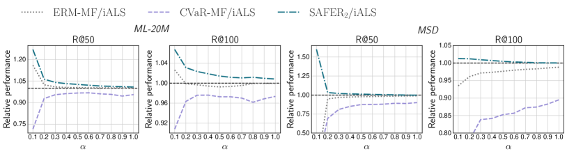
Figure 3: Relative performance of each method over iALS for each quantile level.

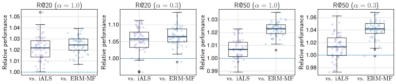
Figure 4: Distributions of relative performances of SAFER₂ over ERM-MF and iALS on ML-1M.

Runtime comparison.

Table 2: Runtime per epoch.

	ML-20M	MSD
Models	Runtime/epoch	Runtime/epoch
iALS	$3.16$ sec	$53.5$ sec
CVaR-MF	$1.67$ sec	$25.2$ sec
SAFER2	$3.45$ sec	$57.0$ sec

The runtime per epoch of each method is shown in Table 2. All experiments are performed using our multi-threaded C++ implementation, originally provided by Rendle et al. [2022], which utilises Eigen to perform vector/matrix operations that support AVX instructions. The reported numbers are the averaged runtime through 50 epochs measured using a GCP instance equipped with 86.4 GB RAM and Intel(R) Xeon(R) CPU @ 2.00GHz with 96 CPU cores (i.e. n1-highcpu-96). The runtime of SAFER₂ is highly competitive to iALS, which is the most efficient CF method. CVaR-MF is faster than SAFER₂ and iALS in terms of runtime per epoch because it is free from the cubic dependency on $d$. However, as shown in Figure 6, CVaR-MF requires much more training epochs to obtain acceptable performance; it has not converged yet even with $50$ epochs while iALS and SAFER₂ converge with around $10$ epochs; each point on each curve of CVaR-MF corresponds to the model after $50$ epochs. These results show that SAFER₂ enables efficient optimisation in terms of both runtime and convergence speed.

Convergence profile.

Lacking a theoretical convergence guarantee, we empirically investigate the training behaviour of SAFER₂. Figure 6 demonstrates the effect of bandwidth $h$ on the convergence profile of SAFER₂. The top row of the figures shows the residual norms of each block at each step, while the bottom row illustrates the validation measures. We observe that setting a small bandwidth (i.e. $h=0.01,0.05$) impedes convergence; in particular, the case with $h=0.01$, which almost degenerates to the non-smooth CVaR, experiences large fluctuation in residual norms and ranking quality. By contrast, a sufficiently large value of $h$ (i.e. $h=0.18,1\mathrm{e}{16}$) ensures stable convergence, whereas $h=1\mathrm{e}{16}$, which is reduced to ERM, does not achieve optimal performance in semi-worst-case scenarios. These results support that convolution-type smoothing is vital for ensuring stable convergence and semi-worst-case performance in SAFER₂.

Figure 5: Ranking quality vs. training epochs and wall time on ML-20M (top) and MSD (bottom).

Figure 6: Convergence profile of SAFER₂ with different bandwidth $h$ on ML-20M.

6 Conclusion

Towards the modernisation of industrial recommender systems, where the engagement of tail users is vital for business growth, we presented a practical algorithm that ensures high-quality personalisation for each individual user while maintaining scalability for real-world web applications. Our algorithm, called SAFER₂, overcomes non-smoothness and non-separability problems in CVaR minimisation by using convolution-type smoothing which is the essential ingredient to obtain its separable reformulation and attain scalability over two dimensions of users and items. Compared to the celebrated iALS, our SAFER₂ is scalable to the same extent yet exhibits superior robustness in terms of semi-worst-case performance while still maintaining average quality. Although we have observed promising empirical results on the convergence behaviour of SAFER₂ in this paper, SAFER₂ lacks theoretical convergence guarantees, which we intend to investigate further in future work.

Appendix

Appendix A Convex and separable upper bound

We first derive the convex upper bound of the loss function in Eq. Pairwise Loss.

$$\frac{1}{|\mathcal{V}_{i}|}\sum_{j\in\mathcal{V}_{i}}\sum_{j^{\prime}\in\mathcal{V}}\mathds{1}\{f_{\theta}(i,j^{\prime})\geq f_{\theta}(i,j)\},$$ (9)

$$\leq \frac{1}{|\mathcal{V}_{i}|}\sum_{j\in\mathcal{V}_{i}}\sum_{j^{\prime}\in\mathcal{V}}\max(0,f_{\theta}(i,j^{\prime})-f_{\theta}(i,j)+1)$$ (10)

$$\leq \frac{1}{|\mathcal{V}_{i}|}\sum_{j\in\mathcal{V}_{i}}\sum_{j^{\prime}\in\mathcal{V}}\left[f_{\theta}(i,j^{\prime})-f_{\theta}(i,j)+1\right]^{2}.$$ (11)

Note that we used $(x+1)^{2}\geq\mathds{1}\{x\geq 0\}$ to obtain the third inequality.

We next derive a separable upper bound of the above loss as follows:

$$\frac{1}{|\mathcal{V}_{i}|}\sum_{j\in\mathcal{V}_{i}}\sum_{j^{\prime}\in\mathcal{V}}\left[f_{\theta}(i,j^{\prime})-f_{\theta}(i,j)+1\right]^{2}$$ (12)

$$\leq \frac{1}{|\mathcal{V}_{i}|}\sum_{j\in\mathcal{V}_{i}}\sum_{j^{\prime}\in\mathcal{V}}\left(1-\left[f_{\theta}(i,j)\right]^{2}+f_{\theta}(i,j^{\prime})^{2}\right)$$ (13)

$$= \frac{1}{|\mathcal{V}_{i}|}\sum_{j\in\mathcal{V}_{i}}\left(|\mathcal{V}|\cdot\left[1-f_{\theta}(i,j)\right]^{2}+\sum_{j\in\mathcal{V}}f_{\theta}(i,j)^{2}\right)$$ (14)

$$\leq |\mathcal{V}|\cdot\left(\frac{1}{|\mathcal{V}_{i}|}\sum_{j\in\mathcal{V}_{i}}\left[1-f_{\theta}(i,j)\right]^{2}+\frac{\mu}{|\mathcal{V}|}\cdot\sum_{j\in\mathcal{V}}f_{\theta}(i,j)^{2}\right),$$ (15)

where $\mu\geq 1$ is a hyperparameter. By substituting $\beta_{0}=\mu/|\mathcal{V}|\geq 1/|\mathcal{V}|$, we obtain our proposed loss. The second term on the RHS of the final inequality is known as the implicit regulariser [Bayer et al., 2017] and the gravity term [Krichene et al., 2018].

Appendix B Implicit Alternating Least Squares (iALS)

In this appendix, we provide a brief description of iALS [Hu et al., 2008; Rendle et al., 2022]. The objective of iALS can be considered as a variant of ERM-MF, which is defined as follows:

$$\min_{\mathbf{U},\mathbf{V}}\sum_{i\in\mathcal{U}}\ell_{\text{iALS}}(\mathbf{V}\mathbf{u}_{i},\mathcal{V}_{i})+\Omega(\mathbf{U},\mathbf{V}),$$ (iALS)

where

$$\ell_{\text{iALS}}(\mathbf{V}\mathbf{u}_{i},\mathcal{V}_{i})\coloneqq\sum_{j\in\mathcal{V}_{i}}\frac{1}{2}(\mathbf{u}_{i}^{\top}\mathbf{v}_{j}-1)^{2}+\frac{\beta_{0}}{2}\|\mathbf{V}\mathbf{u}_{i}\|_{2}^{2}.$$ (Unnormalised Implicit MF)

Observe that iALS’s loss function is unnormalised for each user in contrast to the loss in Eq. Implicit MF. Using this, iALS solves the above optimisation problem by alternatingly solving the block-wise subproblems as follows:

$$\mathbf{U}^{(t+1)} =\operatorname*{argmin}_{\mathbf{U}}\left\{\sum_{i\in\mathcal{U}}\ell_{\text{iALS}}(\mathbf{V}^{(t)}\mathbf{u}_{i},\mathcal{V}_{i})+\frac{1}{2}\|\mathbf{\Lambda}_{u}^{1/2}\mathbf{U}\|_{F}^{2}\right\},$$ (16)

$$\mathbf{V}^{(t+1)} =\operatorname*{argmin}_{\mathbf{V}}\left\{\sum_{i\in\mathcal{U}}\ell_{\text{iALS}}(\mathbf{V}\mathbf{u}_{i}^{(t+1)},\mathcal{V}_{i})+\frac{1}{2}\|\mathbf{\Lambda}_{v}^{1/2}\mathbf{V}\|_{F}^{2}\right\}.$$ (17)

Each subproblem is row-wise separable, and we can obtain a closed-form update for each row of $\mathbf{U}$ and $\mathbf{V}$ by solving the following linear systems,

$$\left(\sum_{j\in\mathcal{V}_{i}}\mathbf{v}_{j}^{(t)}\otimes\mathbf{v}_{j}^{(t)}+\beta_{0}\sum_{j\in\mathcal{V}}\mathbf{v}_{j}^{(t)}\otimes\mathbf{v}_{j}^{(t)}+\lambda_{u}^{(i)}\mathbf{I}\right)\mathbf{u}_{i} =\sum_{j\in\mathcal{V}_{i}}\mathbf{v}_{j}^{(t)},$$ (18)

$$\left(\sum_{i\in\mathcal{U}_{j}}\mathbf{u}_{i}^{(t+1)}\otimes\mathbf{u}_{i}^{(t+1)}+\beta_{0}\sum_{i\in\mathcal{U}}\mathbf{u}_{i}^{(t+1)}\otimes\mathbf{u}_{i}^{(t+1)}+\lambda_{v}^{(j)}\mathbf{I}\right)\mathbf{v}_{j} =\sum_{i\in\mathcal{U}_{j}}\mathbf{u}_{i}^{(t+1)},$$ (19)

where $\mathbf{x}\otimes\mathbf{x}=\mathbf{x}\mathbf{x}^{\top}$ is the outer product operator. Various regularisation strategies have been proposed for iALS [Zhou et al., 2008; Rendle et al., 2022]. Rendle et al. [2022] proposed the following weighting strategy,

$$(\mathbf{\Lambda}_{u})_{i,i}=\lambda_{u}^{(i)}=\lambda\left(|\mathcal{V}_{i}|+\beta_{0}|\mathcal{V}|\right)^{\nu},\quad(\mathbf{\Lambda}_{v})_{j,j}=\lambda_{v}^{(j)}=\lambda\left(|\mathcal{U}_{j}|+\beta_{0}|\mathcal{U}|\right)^{\nu}.$$ (iALS-Reg)

In this paper, we consider $\nu=1$ as recently suggested by Rendle et al. [2022].

Appendix C Convolution-type smoothing

C.1 Definition and derivatives

We define the ramp function $\rho_{1}(\cdot)$ and the check function $\rho_{\tau}(\cdot)$ for $\tau\in(0,1)$ as follows:

$$\rho_{1}(u)=\begin{cases}0,&u\leq 0\\ u,&u>0\end{cases}\ \ \ \ \ \mathrm{and}\ \ \ \ \ \ \rho_{\tau}(u)=\begin{cases}(\tau-1)u,&u\leq 0\\ \tau u,&u>0\end{cases}.$$ (20)

Given $\alpha\in(0,1)$, we consider the convolution function $(\rho_{1-\alpha}\ast k_{h})$ with the kernel density function $k_{h}(\cdot)\coloneqq h^{-1}k(\cdot/h)$ with bandwidth $h>0$. We can show that

$$(\rho_{1-\alpha}\ast k_{h})(u) =\int\rho_{1-\alpha}(v)k_{h}(v-u)dv$$

$$=-\alpha\int_{-\infty}^{0}v\cdot k_{h}(v-u)dv+(1-\alpha)\int_{0}^{\infty}v\cdot k_{h}(v-u)dv$$

$$=-\alpha\int_{-\infty}^{\infty}v\cdot k_{h}(v-u)dv+\int_{0}^{\infty}v\cdot k_{h}(v-u)dv$$

$$=-\alpha\int_{-\infty}^{\infty}(t+u)\cdot k_{h}(t)dt+\int_{-u}^{\infty}(t+u)\cdot k_{h}(t)dt,$$

where an application of a change of variables yields the last equality. Then, we can obtain the first derivative of the convolution function as follows:

$$\nabla_{u}(\rho_{1-\alpha}\ast k_{h})(u) =-\alpha\int_{-\infty}^{\infty}k_{h}(t)dt+\int_{-u}^{\infty}k_{h}(t)dt$$

$$=-\alpha+\left(1-\int_{-\infty}^{-u}k_{h}(t)dt\right)$$

$$=(1-\alpha)-K_{h}(-u).$$

Also, we can obtain the second derivative

$$\nabla_{u}^{2}(\rho_{1-\alpha}\ast k_{h})(u) =k_{h}(-u).$$

C.2 Interpretation

In this subsection, we offer a general understanding of convolution smoothing as a kernel density estimation for the underlying errors. Let $y$ be a continuous random variable having the density function $f_{y}$. We consider the problem of predicting $y$ by a parametric model $g_{\theta}(x)$ with parameters $\theta$ and predictors $x$. Given some function $\rho:\mathbb{R}\to[0,\infty)$, we consider a population minimisation problem,

$$\min_{\theta}\mathbb{E}[\rho(y-g_{\theta}(x))].$$ (21)

Applying the change of variables, we can show that

$$\mathbb{E}[\rho(y-g_{\theta}(x))] =\int\rho(y-g_{\theta}(x))f_{y}(y)dy$$ (22)

$$=\int\rho(v)f_{u}(v;\theta)dv,$$ (23)

where $f_{u}(v;\theta)\coloneqq f_{y}(v+g_{\theta}(x))$ can be considered as a density of $u(\theta)\coloneqq y-g_{\theta}(x)$.

Given finite samples $\{(x_{i},y_{i})\}_{i=1}^{n}$ with the sample size being $n$, we can non-parametrically estimate the density $f_{u}(v;\theta)$ by the kernel estimator, defined by

$$\widehat{f}_{u}(v;\theta)\coloneqq\frac{1}{n}\sum_{i=1}^{n}k_{h}(v-u_{i}(\theta)),$$ (24)

with a kernel density function $k_{h}(\cdot)\coloneqq h^{-1}k(\cdot/h)$ with bandwidth $h>0$. Then, we can write the finite-sample counterpart of the objective function as

$$\int\rho(v)\widehat{f}_{u}(v;\theta)dv =\frac{1}{n}\sum_{i=1}^{n}\int\rho(v)k_{h}(v-u_{i}(\theta))dv$$ (25)

$$=\frac{1}{n}\sum_{i=1}^{n}(\rho\ast k_{h})(u_{i}(\theta)),$$ (26)

where the last equality is due to the definition of convolution-type smoothing. The result above show that the convolution smoothing can be interpreted as a kernel density estimation technique for approximating the distribution of underlying errors.

C.3 On the convolution-type smoothing for CVaR

Proposition C.1.

If the kernel function $k_{h}$ is symmetric, the subproblem of $\xi$ is equivalent to the following,

$$\min_{\xi}\left\{\sum_{i\in\mathcal{U}}\left[(\rho_{1-\alpha}\ast k_{h})(\ell(\mathbf{V}\mathbf{u}_{i},\mathcal{V}_{i})-\xi)\right]\right\},$$

where $\rho_{1-\alpha}(u)=(1-\alpha-\mathds{1}\{u<0\})u$.

Proof.

We show that, if the kernel function $k_{h}$ is symmetric, the following equality holds,

$$\xi+(\rho_{1}\ast k_{h})(y-\xi)=y+\frac{1}{\alpha}(\rho_{1-\alpha}\ast k_{h})(y-\xi).$$ (27)

From the definition of the convolution operator, we have

$$(\rho_{1}\ast k_{h})(u)=\int\max(0,v)\cdot k_{h}(v-u)dv=\int_{0}^{\infty}v\cdot k_{h}(v-u)dv,$$ (28)

which implies

$$\xi+\frac{1}{\alpha}(\rho_{1}\ast k_{h})(y-\xi)=\xi+\frac{1}{\alpha}\int_{0}^{\infty}v\cdot k_{h}(v-\{y-\xi\})dv.$$ (CtS-CVaR)

Here, we also have

$$(\rho_{1-\alpha}\ast k_{h})(u) =-\alpha\int_{-\infty}^{\infty}v\cdot k_{h}(v-u)dv+\int_{0}^{\infty}v\cdot k_{h}(v-u)dv.$$ (29)

It follows that

$$y-\xi+\frac{1}{\alpha}(\rho_{1-\alpha}\ast k_{h})(y-\xi) =y-\xi-\int_{-\infty}^{\infty}v\cdot k_{h}(v-\{y-\xi\})dv+\frac{1}{\alpha}\int_{0}^{\infty}v\cdot k_{h}(v-\{y-\xi\})dv$$ (30)

$$=\int_{-\infty}^{\infty}(u-v)\cdot k_{h}(v-\{y-\xi\})dv+\frac{1}{\alpha}\int_{0}^{\infty}v\cdot k_{h}(v-\{y-\xi\})dv$$ (31)

$$=\frac{1}{\alpha}\int_{0}^{\infty}v\cdot k_{h}(v-\{y-\xi\})dv,$$ (CtS-QE)

where the second equality is due to that $\int_{-\infty}^{\infty}k_{h}(v-\{y-\xi\})dv=1$ and the third equality is due to the symmetric kernel. By combining Eq. CtS-CVaR and Eq. CtS-QE, we have

$$\xi+\frac{1}{\alpha}(\rho_{1}\ast k_{h})(y-\xi)=\xi+y-\xi+\frac{1}{\alpha}(\rho_{1-\alpha}\ast k_{h})(y-\xi)$$ (32)

$$\Longleftrightarrow \xi+\frac{1}{\alpha}(\rho_{1}\ast k_{h})(y-\xi)=y+\frac{1}{\alpha}(\rho_{1-\alpha}\ast k_{h})(y-\xi),$$ (33)

which completes the proof. ∎

ERM-QE Decomposition.

The above observation immediately implies Proposition C.1,

$$\underbrace{\xi+\frac{1}{\alpha|\mathcal{U}|}\sum_{i\in\mathcal{U}}(\rho_{1}\ast k_{h})(\ell(\mathbf{V}\mathbf{u}_{i},\mathcal{V}_{i})-\xi)}_{\Psi_{1-\alpha}(\mathbf{U},\mathbf{V},\xi)}=\underbrace{\frac{1}{|\mathcal{U}|}\sum_{i\in\mathcal{U}}\ell(\mathbf{V}\mathbf{u}_{i},\mathcal{V}_{i})}_{\text{ERM}}+\underbrace{\frac{1}{\alpha|\mathcal{U}|}\sum_{i\in\mathcal{U}}(\rho_{1-\alpha}\ast k_{h})(\ell(\mathbf{V}\mathbf{u}_{i},\mathcal{V}_{i})-\xi)}_{\text{Smoothed quantile estimation}}.$$ (34)

This result is also interesting in the sense that the CVaR objective $\Psi_{1-\alpha}(\mathbf{U},\mathbf{V},\xi)$ can be decomposed into the objectives of ERM and smoothed quantile estimation. However, we do not use the RHS for the update of $\mathbf{U}$ and $\mathbf{V}$ because the term of smoothed quantile estimation is not block convex because $\rho_{1-\alpha}(u)$ is convex but decreasing in $u<0$; See also Figure 2.

C.4 Properties of convolution-type smoothed check functions

We here discuss the properties of smoothed check functions assumed to derive SAFER₂.

Property C.2.

For any bandwidth $h>0$ and any quantile level $\alpha\in[0,1]$, the smoothed check function $(\rho_{1}\ast k_{h})$ satisfies the following properties:

1. $(\rho_{1}\ast k_{h})$ is non-decreasing.

2. $(\rho_{1}\ast k_{h})$ is closed if the loss function $\ell$ and smoothed quantile $\xi$ take finite values.

3. $(\rho_{1}\ast k_{h})$ is strictly convex if the kernel function $k_{h}$ has the full support.

Proof.

The first derivative of the smoothed check function is $\nabla_{u}(\rho_{1}\ast k_{h})(u)=1-K_{h}(-u)$, and therefore, it is non-negative based on the definition of the CDF $K_{h}$. This implies (1). By satisfying the assumptions where (a) the function $(\rho_{1-\alpha}\ast k_{h})$ is continuous and (b) its domain $\mathrm{dom}(\rho_{1-\alpha}\ast k_{h})$ is closed, (2) holds. Moreover, since the second derivative of the smoothed check function is the density function (i.e. $\nabla_{u}^{2}(\rho_{1-\alpha}\ast k_{h})(u)=k_{h}(u)$), if $k_{h}(u)>0$ holds for the domain of $u$, then (3) immediately follows. ∎

In (1), we confirm that the smoothed check function maintains the non-decreasing property. Consequently, the composite function $(\rho_{1}\ast k_{h})\circ\ell$ preserves block convexity if $\ell$ is block convex. By using (1)-(2), the biconjugate of $(\rho_{1}\ast k_{h})$ is $(\rho_{1}\ast k_{h})$ itself [Boyd and Vandenberghe, 2004], enabling the separable reformulation in Eq. PD-Splitting; note that the assumptions of finite $\ell$ and $\xi$ for (2) may not be stringent conditions in practice. (3) implies that the Newton–Raphson method in the $\xi$ step may require full-support kernels, such as logistic and Gaussian kernels. However, we can still use the kernels with the support on $(-1,1)$, such as uniform and Epanechnikov kernels, by using a sufficiently large bandwidth, which allows us to expand the support on $(-h,h)$; we further discuss the instantiation of SAFER₂ with such kernel functions in Section D.3.

1 $\forall i\in\mathcal{U},~{}\mathbf{u}_{i}\sim\mathcal{N}(\vec{0},(\sigma/\sqrt{d})\mathbf{I}_{d}),\quad\forall j\in\mathcal{V},~{}\mathbf{v}_{j}\sim\mathcal{N}(\vec{0},(\sigma/\sqrt{d})\mathbf{I}_{d})$

2 $\xi\leftarrow 0$

3 for $t\leftarrow 1$ to $T$ do

4       $\mathbf{G}_{V}\leftarrow\mathbf{V}^{\top}\mathbf{V}=\sum_{j\in\mathcal{V}}\mathbf{v}_{j}\mathbf{v}_{j}^{\top}$

5       Compute $\forall i\in\mathcal{U},\,\ell_{i}=\frac{1}{2|\mathcal{V}_{i}|}\sum_{j\in\mathcal{V}_{i}}(1-\mathbf{u}_{i}^{\top}\mathbf{v}_{j})^{2}+\frac{\beta_{0}}{2}\cdot\mathbf{u}_{i}^{\top}\mathbf{G}_{V}\mathbf{u}_{i}$

6       for $l\leftarrow 1$ to $L$ do

7             Uniformly draw $\mathcal{U}_{b}\subseteq\mathcal{U}$

8             $\widehat{d}\leftarrow\frac{\nabla_{\xi}\widehat{\Psi}_{1-\alpha}(\mathbf{U},\mathbf{V},\xi)}{\nabla_{\xi}^{2}\widehat{\Psi}_{1-\alpha}(\mathbf{U},\mathbf{V},\xi)}$

9             $\gamma\leftarrow\operatorname*{argmax}_{\gamma\in(0,1)}\gamma$

10               s.t. $\widehat{\Psi}_{1-\alpha}(\mathbf{U},\mathbf{V},\xi-\gamma\widehat{d})\leq\widehat{\Psi}_{1-\alpha}(\mathbf{U},\mathbf{V},\xi)-c\gamma\widehat{d}\nabla_{\xi}\widehat{\Psi}_{1-\alpha}(\mathbf{U},\mathbf{V},\xi-\gamma\widehat{d})$

11             $\xi\leftarrow\xi-\gamma\cdot\widehat{d}$

12       end for

13      for $i\leftarrow 1$ to $|\mathcal{U}|$ do

14             $z_{i}\leftarrow 1-K_{h}(\xi-\ell_{i})$

15             $\mathbf{u}_{i}\leftarrow\left(\frac{z_{i}}{|\mathcal{V}_{i}|}\sum_{j\in\mathcal{V}_{i}}\mathbf{v}_{j}\mathbf{v}_{j}^{\top}+z_{i}\beta_{0}\mathbf{G}_{V}+\alpha|\mathcal{U}|\lambda_{u}^{(i)}\mathbf{I}_{d}\right)^{-1}\frac{z_{i}}{|\mathcal{V}_{i}|}\sum_{j\in\mathcal{V}_{i}}\mathbf{v}_{j}$

16       end for

17      $\widetilde{\mathbf{G}}_{U}\leftarrow\mathbf{U}^{\top}\text{diagMat}(\mathbf{z})\mathbf{U}$

18       for $j\leftarrow 1$ to $|\mathcal{V}|$ do

19             $\mathbf{v}_{j}\leftarrow\left(\sum_{i\in\mathcal{U}_{j}}\frac{z_{i}}{|\mathcal{V}_{i}|}\mathbf{u}_{i}\mathbf{u}_{i}^{\top}+\beta_{0}\widetilde{\mathbf{G}}_{U}+\alpha|\mathcal{U}|\lambda_{v}^{(j)}\mathbf{I}_{d}\right)^{-1}\sum_{i\in\mathcal{U}_{j}}\frac{z_{i}}{|\mathcal{V}_{i}|}\mathbf{u}_{i}$

20       end for

21      

22 end for

Algorithm 3 SAFER₂ solver.

Appendix D Detailed implementation of SAFER₂

This appendix provides a detailed description of SAFER₂, including its various instances of SAFER₂ for kernel functions. Furthermore, we shall detail a variant of SAFER₂ for a large embedding size, utilising the subspace-based block coordinate descent as introduced by Rendle et al. [2021].

Alternating optimisation.

SAFER₂ updates each block cyclically as follows:

$$\xi^{(t+1)} =\operatorname*{argmin}_{\xi}\left\{\xi+\frac{1}{\alpha|\mathcal{U}|}\sum_{i\in\mathcal{U}}(\rho_{1}\ast k_{h})(\ell(\mathbf{V}^{(t)}\mathbf{u}_{i}^{(t)},\mathcal{V}_{i})-\xi)\right\},$$

$$\mathbf{z}^{(t+1)} =\operatorname*{argmax}_{\mathbf{z}}\left\{\sum_{i\in\mathcal{U}}\left[z_{i}\cdot(\ell(\mathbf{V}^{(t)}\mathbf{u}_{i}^{(t)},\mathcal{V}_{i})-\xi^{(t+1)})-(\rho_{1}\ast k_{h})^{*}\left(z_{i}\right)\right]\right\},$$

$$\mathbf{U}^{(t+1)} =\operatorname*{argmin}_{\mathbf{U}}\left\{\frac{1}{\alpha|\mathcal{U}|}\sum_{i\in\mathcal{U}}\left[z_{i}^{(t+1)}\cdot\ell(\mathbf{V}^{(t)}\mathbf{u}_{i},\mathcal{V}_{i})\right]+\frac{1}{2}\|\mathbf{\Lambda}_{u}^{1/2}\mathbf{U}\|_{F}^{2}\right\},$$

$$\mathbf{V}^{(t+1)} =\operatorname*{argmin}_{\mathbf{V}}\left\{\frac{1}{\alpha|\mathcal{U}|}\sum_{i\in\mathcal{U}}\left[z_{i}^{(t+1)}\cdot\ell(\mathbf{V}\mathbf{u}_{i}^{(t+1)},\mathcal{V}_{i})\right]+\frac{1}{2}\|\mathbf{\Lambda}_{v}^{1/2}\mathbf{V}\|_{F}^{2}\right\}.$$

Below, we present an efficient implementation of each step. The overall algorithm is described in Algorithm 3, including the update formulae for $\mathbf{U}$ and $\mathbf{V}$.

D.1 Convolution-type smoothed quantile estimation

Newton–Raphson algorithm.

The subproblem of $\xi$ for the general kernel density function $k_{h}$ cannot be solved analytically. Hence, we resort to a numerical solution using the efficient Newton–Raphson (NR) method. At the $l$-th iteration in the $(t+1)$-th update, we estimate $\xi$ as follows:

$$\xi_{l+1}^{(t+1)}=\xi_{l}^{(t+1)}-\gamma_{l}\cdot d_{l}^{(t+1)},\quad\text{where}~{}d_{l}^{(t+1)}=\frac{\nabla_{\xi}\Psi_{1-\alpha}(\mathbf{U}^{(t)},\mathbf{V}^{(t)},\xi)}{\nabla_{\xi}^{2}\Psi_{1-\alpha}(\mathbf{U}^{(t)},\mathbf{V}^{(t)},\xi)}.$$ (35)

Here, the first and second derivatives of $(1-\alpha)$-CtS-CVaR can be evaluated as follows:

$$\nabla_{\xi}\Psi_{1-\alpha}(\mathbf{U},\mathbf{V},\xi) =-\frac{1}{\alpha|\mathcal{U}|}\sum_{i\in\mathcal{U}}[(1-\alpha)-K_{h}(\xi-\ell(\mathbf{V}\mathbf{u}_{i},\mathcal{V}_{i}))],$$ (36)

$$\nabla_{\xi}^{2}\Psi_{1-\alpha}(\mathbf{U},\mathbf{V},\xi) =\frac{1}{\alpha|\mathcal{U}|}\sum_{i\in\mathcal{U}}k_{h}(\xi-\ell(\mathbf{V}\mathbf{u}_{i},\mathcal{V}_{i})).$$ (37)

Pre-computing the loss $\ell(\mathbf{V}\mathbf{u}_{i},\mathcal{V}_{i})$ for each user can be helpful in reducing the computational burden when the gradient and Hessian can be computed exactly. Furthermore, an effective initialisation of $\xi$ is crucial, and we set $\xi_{0}^{t+1}$ to the previous estimate, i.e. $\xi_{0}^{t+1}=\xi_{L}^{t}$.

Backtracking line search.

The value of $\gamma$ plays a vital role in obtaining an accurate solution for $\xi$. However, a constant $\gamma$ often fails to provide efficient results. One way to overcome this is by employing the widely-used backtracking line search to determine $\xi$ adaptively. It aims to find the maximum $\gamma\in\{1/2,1/4,\dots\}$ such that the Armijo (sufficient decrease) condition [Armijo, 1966] is satisfied. We can express this as:

$$\gamma^{\ast}= \max_{\gamma\in\{1/2,1/4,\dots,\}}\gamma,$$ (38)

$$\text{s.t.}~{}\Psi_{1-\alpha}(\mathbf{U},\mathbf{V},\xi-\gamma\cdot d)\leq\Psi_{1-\alpha}(\mathbf{U},\mathbf{V},\xi)-c\gamma d\cdot\nabla_{\xi}\Psi_{1-\alpha}(\mathbf{U},\mathbf{V},\xi-\gamma\cdot d),$$ (39)

where $c>0$ is the error tolerance parameter, often set to a small value such as $10^{-4}$. Performing each iteration of backtracking line search for evaluating $\Psi_{1-\alpha}(\mathbf{U},\mathbf{V},\xi-\gamma\cdot d)$ takes the cost of $\mathcal{O}(|\mathcal{U}|)$. Therefore, this step demands a cost of $\mathcal{O}(|\mathcal{U}|L)$ for each epoch.

Sub-sampled algorithm.

Although the computation of the direction $d$ can be done in parallel for users, it may be costly for many users, particularly when using a backtracking line search with the cost of $\mathcal{O}(|\mathcal{U}|L)$. We can introduce the sub-sampled Newton–Raphson method [Roosta-Khorasani and Mahoney, 2019] to reduce this cost by approximating the gradient and Hessian based on the uniformly sub-sampled users. Let $|\mathcal{U}_{b}|$ be the sub-sample size of users, which is smaller than the original users size $|\mathcal{U}|$. Chernozhukov and Fernández-Val [2005] obtain the large-sample properties of the quantile regression estimator based on sub-sampling, under the setting where $|\mathcal{U}_{b}|/|\mathcal{U}|\to 0$ and $|\mathcal{U}_{b}|\to\infty$ as $|\mathcal{U}|\to\infty$. Their results suggest that the sub-sample estimator $\hat{\xi}_{b}$ of the true value $\xi_{0}$ satisfies that $\hat{\xi}_{b}=\xi_{0}+O_{p}(1/\sqrt{|\mathcal{U}_{b}|})$. That is, the sub-sample estimator converges to the true parameter at a rate of $1/\sqrt{|\mathcal{U}_{b}|}$. In practice, the user size is often larger than ten million or more, and the sub-sample size $|\mathcal{U}_{b}|=100{,}000$ ensures that the estimation error asymptotically vanishes as $1/\sqrt{|\mathcal{U}_{b}|}\approx 0.00316$.

D.2 Re-weighted ALS

The update of $\mathbf{U}$ and $\mathbf{V}$ can be reformulated by using primal-dual splitting as in Eq. PD-Splitting. Here, we focus on the update of primal variables, i.e. $\mathbf{U}$ and $\mathbf{V}$, since we have already described the $\mathbf{z}$ step in Section 3.3,

$\mathbf{U}$ step.

Given $\mathbf{z}$, the optimisation problem of $\mathbf{U}$ and $\mathbf{V}$ forms a re-weighted ERM. Owing to separability, the update of $\mathbf{U}$,

$$\mathbf{U}^{(t+1)} =\operatorname*{argmin}_{\mathbf{U}}\left\{\frac{1}{\alpha|\mathcal{U}|}\sum_{i\in\mathcal{U}}[z_{i}^{(t+1)}\cdot\ell(\mathbf{V}^{(t)}\mathbf{u}_{i},\mathcal{V}_{i})]+\frac{1}{2}\|\mathbf{\Lambda}_{u}^{1/2}\mathbf{U}\|_{F}^{2}\right\},$$ (40)

can be solved in parallel with respect to each row $\mathbf{u}_{i}$ as follows:

$$\frac{z_{i}^{(t+1)}}{\alpha|\mathcal{U}|}\nabla_{\mathbf{u}_{i}}\ell(\mathbf{V}^{(t)}\mathbf{u}_{i},\mathcal{V}_{i})+\lambda_{u}^{(i)}\mathbf{u}_{i}=0$$ (41)

$$\Longleftrightarrow \Biggl{(}\frac{z_{i}^{(t+1)}}{|\mathcal{V}_{i}|}\underbrace{\sum_{j\in\mathcal{V}_{i}}\mathbf{v}_{j}^{(t)}\otimes\mathbf{v}_{j}^{(t)}}_{\text{(a)}}+z_{i}^{(t+1)}\beta_{0}\underbrace{\sum_{j\in\mathcal{V}}\mathbf{v}_{j}^{(t)}\otimes\mathbf{v}_{j}^{(t)}}_{\text{(b)}}+\alpha|\mathcal{U}|\lambda_{u}^{(i)}\mathbf{I}\Biggr{)}\mathbf{u}_{i}=\frac{z_{i}^{(t+1)}}{|\mathcal{V}_{i}|}\sum_{j\in\mathcal{V}_{i}}\mathbf{v}_{j}^{(t)}.$$ (42)

The updated $\mathbf{u}_{i}$ can be obtained by solving the linear system above. Since the user-independent Gramian matrix indicated by (b) has been pre-computed (at a cost of $\mathcal{O}(|\mathcal{V}|d^{2})$), the computational cost of updating each user’s $\mathbf{u}_{i}$ involves computing the user-dependent partial Hessian indicated by (a) in $\mathcal{O}(|\mathcal{V}_{i}|d^{2})$ and then solving a linear system of $d\times d$ in $\mathcal{O}(d^{3})$. Since $\sum_{i\in\mathcal{U}}|\mathcal{V}_{i}|=|\mathcal{S}|$, the total computational cost is thus $\mathcal{O}(|\mathcal{S}|d^{2}+|\mathcal{U}|d^{3})$.

$\mathbf{V}$ step.

Analogously, the update of $\mathbf{V}$,

$$\mathbf{V}^{(t+1)} =\operatorname*{argmin}_{\mathbf{V}}\left\{\frac{1}{\alpha|\mathcal{U}|}\sum_{i\in\mathcal{U}}[z_{i}^{(t+1)}\cdot\ell(\mathbf{V}\mathbf{u}_{i}^{(t+1)},\mathcal{V}_{i})]+\frac{1}{2}\|\lambda_{v}^{1/2}\mathbf{V}\|_{F}^{2}\right\},$$ (43)

can be solved as follows:

$$\nabla_{\mathbf{v}_{j}}\frac{1}{\alpha|\mathcal{U}|}\sum_{i\in\mathcal{U}}z_{i}\cdot\ell(\mathbf{V}\mathbf{u}_{i},\mathcal{V}_{i})+\lambda_{v}^{(j)}\mathbf{v}_{j}=0$$ (44)

$$\Longleftrightarrow \Biggl{(}\sum_{i\in\mathcal{U}_{j}}\frac{z_{i}^{(t+1)}}{|\mathcal{V}_{i}|}\mathbf{u}_{i}^{(t+1)}\otimes\mathbf{u}_{i}^{(t+1)}+\beta_{0}\underbrace{\sum_{i\in\mathcal{U}}z_{i}^{(t+1)}\mathbf{u}_{i}^{(t+1)}\otimes\mathbf{u}_{i}^{(t+1)}}_{\text{(c)}}+\alpha|\mathcal{U}|\lambda_{v}^{(j)}\mathbf{I}\Biggr{)}\mathbf{v}_{j}=\sum_{i\in\mathcal{U}_{j}}\frac{z_{i}^{(t+1)}}{|\mathcal{V}_{i}|}\mathbf{u}_{i}^{(t+1)}.$$ (45)

We can reduce the computational cost of this step as in the $\mathbf{U}$ step by caching the weighted Gramian matrix indicated by (c), which costs $\mathcal{O}(|\mathcal{U}|d^{2})$ when the loss for each user is pre-computed. The computational cost for updating $\mathbf{V}$ is $\mathcal{O}(|\mathcal{S}|d^{2}+|\mathcal{V}|d^{3})$.

D.3 Instantiation of SAFER₂

An instance of SAFER₂ is determined by the choice of the kernel density function $k_{h}$. We shall describe the implementation of SAFER₂ with some popular kernels as it would be helpful for reproducing our method; the implementation described here is available in https://github.com/riktor/safer2-recommender.

Gaussian kernel.

For the Gaussian kernel, the kernel density $k_{h}$ and its CDF $K_{h}$ can be computed as follows:

$$k_{h}(u) =\frac{1}{\sqrt{2\pi}h}\exp\left(-\frac{u^{2}}{2h^{2}}\right),$$ (46)

$$K_{h}(u) =\frac{1}{2}\left[1+\mathrm{erf}\left(\frac{u}{\sqrt{2}h}\right)\right]=\frac{1}{2}\mathrm{erfc}\left(-\frac{u}{\sqrt{2}h}\right),$$ (47)

where $\mathrm{erf}(u)=\frac{2}{\sqrt{\pi}}\int_{0}^{u}\exp(-v^{2})dv$ and $\mathrm{erfc}(u)=1-\mathrm{erf}(u)$ are the error and complementary error functions, respectively.

These complex functions are generally implemented as special functions and can be computed very efficiently [Gautschi, 1970; Poppe and Wijers, 1990; Abrarov and Quine, 2011; Zaghloul and Ali, 2012].

The smoothed check function $(\rho_{1-\alpha}\ast k_{h})$ is then obtained as

$$(\rho_{1-\alpha}\ast k_{h})(u)=\frac{h}{2}\left[h\cdot k_{h}(u)+\frac{u}{h}(1-2\cdot K_{h}(-u))\right]+((1-\alpha)-0.5)u,$$ (48)

which is used for backtracking line-search in the $\xi$ step.

Epanechnikov kernel.

We also describe the implementation for the Epanechnikov kernel [Epanechnikov, 1969]. Epanechnikov kernel density $k_{h}$ and its CDF $K_{h}$ can be computed as follows:

$$k_{h}(u) =\frac{3}{4h}\left[1-\left(\frac{u}{h}\right)^{2}\right]\mathds{1}\{|u/h|\leq 1\},$$ (49)

$$K_{h}(u) =\begin{cases}0,&u<-1\\ \frac{1}{4h^{3}}\left[u(3h^{2}-u^{2})+2h^{3}\right],&u/h\in[-1,1]\\ 1,&u/h>1\end{cases}.$$ (50)

The smoothed check function $(\rho_{1-\alpha}\ast k_{h})$ is then obtained as

$$(\rho_{1-\alpha}\ast k_{h})(u)=\frac{h}{2}\left[\frac{3}{4}\left(\frac{u}{h}\right)^{2}-\frac{1}{8}\left(\frac{u}{h}\right)^{4}+\frac{3}{8}\right]\mathds{1}\{|u/h|\leq 1\}+\frac{h}{2}|u/h|\mathds{1}\{u>1\}+((1-\alpha)-0.5)u.$$ (51)

Note that the support of $k_{h}(u)$ is on $(-h,h)$, and thus we can ensure the strict convexity (i.e. positive Hessian) of $(\rho_{1-\alpha}\ast k_{h})$ in a Newton–Raphson step.

D.4 SAFER₂++

The SAFER₂ algorithm experiences the quadratic/cubic runtime dependency on the embedding size $d$. This problem has been tackled by various studies [Pilászy et al., 2010; He et al., 2016; Bayer et al., 2017], and Rendle et al. [2021] recently reported that the large dimension is very important to obtain the optimal ranking quality of iALS. Considering this, we propose an extension of SAFER₂ for a large embedding size by using the recent subspace-based block coordinate descent of Rendle et al. [2021], which is a simple yet effective approach, enabling efficient utilisation of optimised vector processing units.

Subspace-based block coordinate descent.

To overcome the above problem, iALS++ considers the subvector of a user/item embedding as a block [Rendle et al., 2021] and optimises the subvector by a Newton–Raphson method. We here apply this approach to our SAFER₂. Let $\bm{\pi}\subseteq\{1,\dots,d\}$ be a vector of indices and $\mathbf{u}_{i,\bm{\pi}}$ be the subvector of $\mathbf{u}_{i}$ corresponding to $\bm{\pi}$. Then, the first and second derivatives of the objective $L_{i}(\mathbf{u}_{i},\mathbf{V})=(z_{i}/\alpha|\mathcal{U}|)\cdot\ell(\mathbf{V}\mathbf{u}_{i},\mathcal{V}_{i})+\frac{\lambda_{u}^{(i)}}{2}\|\mathbf{u}_{i}\|_{2}^{2}$ in Eq. PD-Splitting with respect to $\mathbf{u}_{i,\bm{\pi}}$ are:

$$\nabla_{\mathbf{u}_{i,\bm{\pi}}}L_{i}(\mathbf{u}_{i},\mathbf{V}) \propto\frac{z_{i}}{|\mathcal{V}_{i}|}\sum_{j\in\mathcal{V}_{i}}(\mathbf{v}_{j}^{\top}\mathbf{u}_{i}-1)\mathbf{u}_{i,\bm{\pi}}+z_{i}\beta_{0}\left(\sum_{j\in\mathcal{V}}\mathbf{v}_{j,\bm{\pi}}\mathbf{v}_{j}^{\top}\right)\mathbf{u}_{i}+\alpha|\mathcal{U}|\lambda_{u}^{(i)}\mathbf{u}_{i,\bm{\pi}},$$ (52)

$$\nabla_{\mathbf{u}_{i,\bm{\pi}}}^{2}L_{i}(\mathbf{u}_{i},\mathbf{V}) \propto\frac{z_{i}}{|\mathcal{V}_{i}|}\sum_{j\in\mathcal{V}_{i}}\mathbf{v}_{j,\bm{\pi}}\mathbf{v}_{j,\bm{\pi}}^{\top}+z_{i}\beta_{0}\sum_{j\in\mathcal{V}}\mathbf{v}_{j,\bm{\pi}}\mathbf{v}_{j,\bm{\pi}}^{\top}+\alpha|\mathcal{U}|\lambda_{u}^{(i)}\mathbf{I}.$$ (53)

Note that we omitted the constant factor $(\alpha|\mathcal{U}|)^{-1}$ for brevity. We pre-compute the partial Gramian matrices $\sum_{j\in\mathcal{V}}\mathbf{v}_{j,\bm{\pi}}\mathbf{v}_{j}^{\top}$ in $\mathcal{O}(|\mathcal{V}||\bm{\pi}|d)$, $\sum_{j\in\mathcal{V}}\mathbf{v}_{j,\bm{\pi}}\mathbf{v}_{j,\bm{\pi}}^{\top}$ in $\mathcal{O}(|\mathcal{V}||\bm{\pi}|^{2})$, and the prediction $\mathbf{v}_{j}^{\top}\mathbf{u}_{i}$ for $(i,j)\in\mathcal{S}$ in $\mathcal{O}(|\mathcal{S}|d)$. Then, the computational cost of the gradient and Hessian for all users is $\mathcal{O}(|\mathcal{S}||\bm{\pi}|+|\mathcal{U}||\bm{\pi}|d+|\mathcal{S}||\bm{\pi}|^{2})$. We subsequently update the subvector $\mathbf{u}_{i,\bm{\pi}}$ by a Newton–Raphson step,

$$\mathbf{u}_{i,\bm{\pi}}^{(t+1)} =\mathbf{u}_{i,\bm{\pi}}^{(t)}-(\nabla_{\mathbf{u}_{i,\bm{\pi}}}^{2}L_{i}(\mathbf{u}_{i}^{(t)},\mathbf{V}^{(t)}))^{-1}\nabla_{\mathbf{u}_{i,\bm{\pi}}}L_{i}(\mathbf{u}_{i}^{(t)},\mathbf{V}^{(t)}).$$ (54)

This can be computed by solving a linear system of size $|\bm{\pi}|\times|\bm{\pi}|$ in $\mathcal{O}(|\bm{\pi}|^{3})$ time. The computational cost for updating all user subvectors is $\mathcal{O}(|\mathcal{S}||\bm{\pi}|+|\mathcal{V}||\bm{\pi}|d+|\mathcal{S}||\bm{\pi}|^{2}+|\mathcal{U}||\bm{\pi}|^{3})$.

Similarly, denoting $L_{j}(\mathbf{U},\mathbf{V})=(\alpha|\mathcal{U}|)^{-1}\sum_{i\in\mathcal{U}}[z_{i}\cdot\ell(\mathbf{V}\mathbf{u}_{i},\mathcal{V}_{i})]+\frac{\lambda_{v}^{(j)}}{2}\|\mathbf{v}_{j}\|_{2}^{2}$ we can obtain the update of an item embedding as follows:

$$\mathbf{v}_{j,\bm{\pi}}^{(t+1)} =\mathbf{v}_{j,\bm{\pi}}^{(t)}-(\nabla_{\mathbf{v}_{j,\bm{\pi}}}^{2}L_{j}(\mathbf{U},\mathbf{V})^{-1}\nabla_{\mathbf{v}_{j,\bm{\pi}}}L_{i}(\mathbf{U},\mathbf{V}),$$ (55)

where

$$\nabla_{\mathbf{v}_{j,\bm{\pi}}}L_{j}(\mathbf{U},\mathbf{V}) \propto\sum_{i\in\mathcal{U}_{i}}\frac{z_{i}}{|\mathcal{V}_{i}|}(\mathbf{u}_{i}^{\top}\mathbf{v}_{j}-1)\mathbf{v}_{j,\bm{\pi}}+\beta_{0}\left(\sum_{i\in\mathcal{U}}z_{i}\cdot\mathbf{u}_{i,\bm{\pi}}\mathbf{u}_{i}^{\top}\right)\mathbf{v}_{j}+\alpha|\mathcal{U}|\lambda_{v}^{(j)}\mathbf{v}_{j,\bm{\pi}},$$ (56)

$$\nabla_{\mathbf{v}_{j,\bm{\pi}}}^{2}L_{j}(\mathbf{U},\mathbf{V}) \propto\sum_{i\in\mathcal{U}_{j}}\frac{z_{i}}{|\mathcal{V}_{i}|}\mathbf{u}_{i,\bm{\pi}}\mathbf{u}_{i,\bm{\pi}}^{\top}+\beta_{0}\sum_{i\in\mathcal{U}}z_{i}\cdot\mathbf{u}_{i,\bm{\pi}}\mathbf{u}_{i,\bm{\pi}}^{\top}+\alpha|\mathcal{U}|\lambda_{v}^{(j)}\mathbf{I}.$$ (57)

The computational cost for updating all item subvectors is $\mathcal{O}(|\mathcal{S}||\bm{\pi}|+|\mathcal{U}||\bm{\pi}|d+|\mathcal{S}||\bm{\pi}|^{2}+|\mathcal{V}||\bm{\pi}|^{3})$.

Computational complexity.

We follow the iteration scheme suggested by Rendle et al. [2021], which cyclically updates the subspace of user and item sides for each subset of indices. As a result, we obtain the following computational cost

$$\mathcal{O}\left(|\mathcal{S}|d+\frac{d}{|\bm{\pi}|}(|\mathcal{U}|+|\mathcal{V}|)(d|\bm{\pi}|+|\bm{\pi}|^{2}+|\bm{\pi}|^{3})+|\mathcal{S}|(|\bm{\pi}|+|\bm{\pi}|^{2}))\right)$$ (58)

$$\equiv \mathcal{O}(|\mathcal{S}||\bm{\pi}|d+(|\mathcal{U}|+|\mathcal{V}|)(d^{2}+d|\bm{\pi}|^{2})).$$ (59)

The algorithm is shown in Algorithm 4.

1 $\forall i\in\mathcal{U},~{}\mathbf{u}_{i}\sim\mathcal{N}(\vec{0},(\sigma/\sqrt{d})\mathbf{I}_{d}),\quad\forall j\in\mathcal{V},~{}\mathbf{v}_{j}\sim\mathcal{N}(\vec{0},(\sigma/\sqrt{d})\mathbf{I}_{d})$

2 $\xi\leftarrow 0$

3 for $t\leftarrow 1$ to $T$ do

4       $\mathbf{G}_{V}\leftarrow\mathbf{V}^{\top}\mathbf{V}=\sum_{j\in\mathcal{V}}\mathbf{v}_{j}\mathbf{v}_{j}^{\top}$

5       Compute $\forall i\in\mathcal{U},\,\ell_{i}=\frac{1}{2|\mathcal{V}_{i}|}\sum_{j\in\mathcal{V}_{i}}(1-\mathbf{u}_{i}^{\top}\mathbf{v}_{j})^{2}+\frac{\beta_{0}}{2}\cdot\mathbf{u}_{i}^{\top}\mathbf{G}_{V}\mathbf{u}_{i}$

6       for $l\leftarrow 1$ to $L$ do

7             Uniformly draw $\mathcal{U}_{b}\subseteq\mathcal{U}$

8             $\widehat{d}\leftarrow\frac{\nabla_{\xi}\widehat{\Psi}_{1-\alpha}(\mathbf{U},\mathbf{V},\xi)}{\nabla_{\xi}^{2}\widehat{\Psi}_{1-\alpha}(\mathbf{U},\mathbf{V},\xi)}$

9             $\gamma\leftarrow\operatorname*{argmax}_{\gamma\in(0,1)}\gamma$

10               s.t. $\widehat{\Psi}_{1-\alpha}(\mathbf{U},\mathbf{V},\xi-\gamma\widehat{d})\leq\widehat{\Psi}_{1-\alpha}(\mathbf{U},\mathbf{V},\xi)-c\gamma\widehat{d}\nabla_{\xi}\widehat{\Psi}_{1-\alpha}(\mathbf{U},\mathbf{V},\xi-\gamma\widehat{d})$

11             $\xi\leftarrow\xi-\gamma\cdot\widehat{d}$

12       end for

13      for $i\leftarrow 1$ to $|\mathcal{U}|$ do

14             $z_{i}\leftarrow 1-K_{h}(\xi-\ell_{i})$

15       end for

16      for $\bm{\pi}\in\mathcal{P}$ do

17             $\mathbf{G}_{V,\bm{\pi}}^{gl}\leftarrow\sum_{j\in\mathcal{V}}\mathbf{v}_{j,\bm{\pi}}\mathbf{v}_{j}^{\top}$, $\mathbf{G}_{V,\bm{\pi}}^{ll}\leftarrow\sum_{j\in\mathcal{V}}\mathbf{v}_{j,\bm{\pi}}\mathbf{v}_{j,\bm{\pi}}^{\top}$

18             for $i\leftarrow 1$ to $|\mathcal{U}|$ do

19                   $\mathbf{u}_{i,\bm{\pi}}\leftarrow\mathbf{u}_{i}-(\nabla_{\mathbf{u}_{i,\bm{\pi}}}^{2}L_{i}(\mathbf{u}_{i},\mathbf{V}))^{-1}\nabla_{\mathbf{u}_{i,\bm{\pi}}}L_{i}(\mathbf{u}_{i},\mathbf{V})$

20             end for

21            $\widetilde{\mathbf{G}}_{U,\bm{\pi}}^{gl}\leftarrow\sum_{i\in\mathcal{U}}z_{i}\cdot\mathbf{u}_{i,\bm{\pi}}\mathbf{u}_{i}^{\top}$, $\widetilde{\mathbf{G}}_{U,\bm{\pi}}^{ll}\leftarrow\sum_{i\in\mathcal{U}}z_{i}\cdot\mathbf{u}_{i,\bm{\pi}}\mathbf{u}_{i,\bm{\pi}}^{\top}$

22             for $j\leftarrow 1$ to $|\mathcal{V}|$ do

23                   $\mathbf{v}_{j,\bm{\pi}}\leftarrow\mathbf{v}_{j,\bm{\pi}}-(\nabla_{\mathbf{v}_{j,\bm{\pi}}}^{2}L_{j}(\mathbf{U},\mathbf{V}))^{-1}\nabla_{\mathbf{v}_{j,\bm{\pi}}}L_{j}(\mathbf{U},\mathbf{V})$

24             end for

25            

26       end for

27      

28 end for

Algorithm 4 SAFER₂++ solver.

Appendix E On Tikhonov regularisation

In this appendix, we develop a regularisation strategy for SAFER₂, which allows us to control the numerical stability of subproblems for users and items. Since setting appropriate regularisation weight for every user/item is impractical in large-scale settings, we derive a single hyperparameter that controls the regularisation weights for all users and items.

For a matrix $\mathbf{A}\in\mathbb{R}^{d\times d}$, the condition number $\kappa(\mathbf{A})$ is defined as follows:

$$\kappa(\mathbf{A})\coloneqq\|\mathbf{A}^{-1}\|_{F}\cdot\|\mathbf{A}\|_{F}.$$ (60)

The condition number of a matrix $\mathbf{A}$ characterises the numerical stability of a linear system $\mathbf{A}\mathbf{x}=$; this problem with respect to $\mathbf{x}$ is numerically unstable when $\kappa(\mathbf{A})$ is large. We consider normal $\mathbf{A}$, and then the condition number can be computed as follows:

$$\kappa(\mathbf{A})=\frac{|\lambda_{\max}(\mathbf{A})|}{|\lambda_{\min}(\mathbf{A})|},$$ (61)

where $\lambda_{\max}(\mathbf{A})$ and $\lambda_{\min}(\mathbf{A})$ are maximal and minimal eigenvalues of $\mathbf{A}$, respectively. In our case, we want to keep small the condition number of each Hessian matrix with respect to the rows of $\mathbf{U}$ and $\mathbf{V}$. For the $i$-th row of $\mathbf{U}$, the Hessian matrix $\mathbf{H}_{i}$ is as follows:

$$\mathbf{H}_{i}\coloneqq\frac{z_{i}}{|\mathcal{V}_{i}|}\sum_{j\in\mathcal{V}_{i}}\mathbf{v}_{j}\mathbf{v}_{j}^{\top}+z_{i}\beta_{0}\mathbf{V}^{\top}\mathbf{V}+\alpha|\mathcal{U}|\lambda_{u}^{(i)}\mathbf{I},$$ (62)

which implies

$$\lambda_{\min}(\mathbf{H}_{i})=\alpha|\mathcal{U}|\lambda_{u}^{(i)},\quad\lambda_{\max}(\mathbf{H}_{i})=\lambda_{\max}(\mathbf{H}_{i}-\alpha|\mathcal{U}|\lambda_{u}^{(i)}\mathbf{I})+\alpha|\mathcal{U}|\lambda_{u}^{(i)}.$$ (63)

To ensure a small value of $\kappa(\mathbf{H}_{i})$, we can adjust the regularisation weight $\lambda_{u}^{(i)}>0$. However, the maximal eigenvalue $\lambda_{\max}(\mathbf{H}_{i})$ changes at each update step in the alternating optimisation, but computing the dominant eigenvalue is a costly process [Mises and Pollaczek-Geiringer, 1929]. Therefore, we propose a simple regularisation strategy to control the condition number of each linear system solved with a constant hyperparameter. Assuming $\nu>0$ is the upper bound of the squared norm of the user and item embeddings throughout the optimisation, i.e. $\nu\geq\|\mathbf{v}_{j}\|_{2}^{2}$ for all $j\in\mathcal{V}$ and $\nu\geq\|\mathbf{u}_{i}\|_{2}^{2}$ for all $i\in\mathcal{U}$, we have the following upper bound for $\lambda_{\max}(\mathbf{H}_{i}-\alpha|\mathcal{U}|\lambda_{u}^{(i)}\mathbf{I})$:

$$\lambda_{\max}(\mathbf{H}_{i}-\alpha|\mathcal{U}|\lambda_{u}^{(i)}\mathbf{I}) =\left\|\frac{z_{i}}{|\mathcal{V}_{i}|}\sum_{j\in\mathcal{V}_{i}}\mathbf{v}_{j}\mathbf{v}_{j}^{\top}+z_{i}\beta_{0}\mathbf{V}^{\top}\mathbf{V}\right\|_{F}$$ (64)

$$\leq\frac{z_{i}}{|\mathcal{V}_{i}|}\sum_{j\in\mathcal{V}_{i}}\|\mathbf{v}_{j}\|_{2}^{2}+z_{i}\beta_{0}\|\mathbf{V}\|_{F}^{2}$$ (65)

$$\leq z_{i}\nu+z_{i}\beta_{0}|\mathcal{V}|\nu$$ (66)

$$\leq\nu(1+\beta_{0}|\mathcal{V}|).$$ (67)

In the last inequality, we used $z_{i}\leq 1$. Therefore, by setting

$$\lambda_{u}^{(i)}=\frac{\lambda}{\alpha|\mathcal{U}|}\left(1+\beta_{0}|\mathcal{V}|\right)$$ (68)

with a hyperparameter $\lambda>0$, we can ensure

$$\kappa(\mathbf{H}_{i}) =\frac{\lambda_{\max}(\mathbf{H}_{i}-\alpha|\mathcal{U}|\lambda_{u}^{(i)}\mathbf{I})+\lambda_{\min}(\mathbf{H}_{i})}{\lambda_{\min}(\mathbf{H}_{i})}$$ (69)

$$\leq\frac{\nu}{\lambda}+1.$$ (70)

The advantage of this reparametrisation is that we may be able to bound the condition number of each user’s linear system from above by $(\nu/\lambda)+1$, which is independent of $\alpha$, $|\mathcal{U}|$, $|\mathcal{V}_{i}|$ and $i$. Note that a too-large value of $\lambda$ leads to poor model training while the condition number will be close to one, and therefore, we still need to tune $\lambda$.

Analogously, we can derive the regularisation weight for the $j$-th row of $\mathbf{V}$.

$$\mathbf{H}_{j}\coloneqq\sum_{i\in\mathcal{U}_{j}}\frac{z_{i}}{|\mathcal{V}_{i}|}\cdot\mathbf{u}_{i}\mathbf{u}_{i}^{\top}+\beta_{0}\mathbf{U}^{\top}\text{diagMat}(\mathbf{z})\mathbf{U}+\alpha|\mathcal{U}|\lambda_{v}^{(j)}\mathbf{I},$$ (71)

and

$$\lambda_{\max}(\mathbf{H}_{j}-\alpha|\mathcal{U}|\lambda_{v}^{(j)}\mathbf{I}) =\left\|\sum_{i\in\mathcal{U}_{j}}\frac{z_{i}}{|\mathcal{V}_{i}|}\mathbf{u}_{i}\mathbf{u}_{i}^{\top}+\beta_{0}\mathbf{U}^{\top}\text{diagMat}(\mathbf{z})\mathbf{U}\right\|_{F}$$ (72)

$$\leq\sum_{i\in\mathcal{U}_{j}}\frac{z_{i}}{|\mathcal{V}_{i}|}\|\mathbf{u}_{i}\|_{2}^{2}+\beta_{0}\cdot\sum_{i\in\mathcal{U}}z_{i}\|\mathbf{u}_{i}\|_{2}^{2}$$ (73)

$$\leq\nu\cdot\sum_{i\in\mathcal{U}_{j}}\frac{z_{i}}{|\mathcal{V}_{i}|}+\beta_{0}\nu\cdot\sum_{i\in\mathcal{U}}z_{i}$$ (74)

$$\leq\nu\left(\sum_{i\in\mathcal{U}_{j}}\frac{1}{|\mathcal{V}_{i}|}+\beta_{0}\sum_{i\in\mathcal{U}}z_{i}\right).$$ (75)

In contrast to the case of user embeddings, we applied $z_{i}\leq 1$ for the first term of the last inequality. This is because bounding $\sum_{i\in\mathcal{U}}z_{i}\leq|\mathcal{U}|$ is rather loose, and the weighting strategy based on this bound will lead to the over-regularisation of item embeddings. To avoid this, we introduce the following property of convolution-type smoothed quantile.

Proposition E.1.

Suppose that $n$ samples $\{\ell_{1},\dots,\ell_{n}\}$ of losses and its convolution-type smoothed quantile $\xi_{n}\coloneqq\operatorname*{argmin}_{\xi}\sum_{i=1}^{n}(\rho_{1-\alpha}\ast k_{h})(\ell_{i}-\xi)$. Then, $n$ dual variables $\{z_{1},\dots,z_{n}\}$ satisfy

$$\sum_{i=1}^{n}z_{i}=\alpha\cdot n,$$ (76)

where $z_{i}=1-K_{h}(\xi_{n}-\ell_{i})$.

Proof.

The smoothed quantile $\xi_{n}$ satisfies the first-order optimality condition,

$$\nabla_{\xi}\sum_{i=1}^{n}(\rho_{1-\alpha}\ast k_{h})(\ell_{i}-\xi_{n})=0 \Longleftrightarrow\sum_{i=1}^{n}\left[(1-\alpha)-K_{h}(\xi_{n}-\ell_{i})\right]=0$$ (77)

$$\Longleftrightarrow\sum_{i=1}^{n}\left[1-K_{h}(\xi_{n}-\ell_{i})\right]=\alpha\cdot n,$$ (78)

which immediately completes the proof. ∎

From this result, we can substitute $\sum_{i\in\mathcal{U}}z_{i}$ in the upper bound of $\lambda_{\max}(\mathbf{H}_{j}-\alpha|\mathcal{U}|\lambda_{v}^{(j)}\mathbf{I})$ with $\alpha|\mathcal{U}|$ and then obtain

$$\lambda_{\max}(\mathbf{H}_{j}-\alpha|\mathcal{U}|\lambda_{v}^{(j)}\mathbf{I}) \leq\nu\left(\sum_{i\in\mathcal{U}_{j}}\frac{1}{|\mathcal{V}_{i}|}+\beta_{0}\alpha|\mathcal{U}|\right).$$ (79)

By setting

$$\lambda_{v}^{(j)}=\frac{\lambda}{\alpha|\mathcal{U}|}\left(\sum_{i\in\mathcal{U}_{j}}\frac{1}{|\mathcal{V}_{i}|}+\beta_{0}\alpha|\mathcal{U}|\right),$$ (80)

we can ensure

$$\kappa(\mathbf{H}_{j}) =\frac{\lambda_{\max}(\mathbf{H}_{j}-\alpha|\mathcal{U}|\lambda_{v}^{(j)}\mathbf{I})+\lambda_{\min}(\mathbf{H}_{j})}{\lambda_{\min}(\mathbf{H}_{j})}$$ (81)

$$\leq\frac{\nu(\sum_{i\in\mathcal{U}_{j}}\frac{1}{|\mathcal{V}_{i}|}+\beta_{0}\alpha|\mathcal{U}|)}{\alpha|\mathcal{U}|\lambda_{v}^{(j)}}+1$$ (82)

$$=\frac{\nu(\sum_{i\in\mathcal{U}_{j}}\frac{1}{|\mathcal{V}_{i}|}+\beta_{0}\alpha|\mathcal{U}|)}{\lambda(\sum_{i\in\mathcal{U}_{j}}\frac{1}{|\mathcal{V}_{i}|}+\beta_{0}\alpha|\mathcal{U}|)}+1$$ (83)

$$=\frac{\nu}{\lambda}+1.$$ (84)

On the regularisation strategy of iALS.

Tikhonov regularisation has been widely adopted for MF models with the ALS solver [Zhou et al., 2008; Rendle et al., 2022]. In particular, the recent technique in Eq. iALS-Reg (proposed by Rendle et al. [2022]) can be obtained by a similar derivation. Namely, consider the Hessian matrix and regularisation weight for the $i$-th user,

$$\mathbf{H}_{i} =\sum_{j\in\mathcal{V}_{i}}\mathbf{v}_{j}\mathbf{v}_{j}^{\top}+\beta_{0}\mathbf{V}^{\top}\mathbf{V}+\lambda_{u}^{(i)}\mathbf{I},$$ (85)

$$\lambda_{u}^{(i)} =\lambda\left(|\mathcal{V}_{i}|+\beta_{0}|\mathcal{V}|\right),$$ (86)

then we have

$$\lambda_{\max}(\mathbf{H}_{i}-\alpha|\mathcal{U}|\lambda_{u}^{(i)}\mathbf{I}) =\|\sum_{j\in\mathcal{V}_{i}}\mathbf{v}_{j}\mathbf{v}_{j}^{\top}+\beta_{0}\mathbf{V}^{\top}\mathbf{V}\|_{F}$$ (87)

$$\leq\sum_{j\in\mathcal{V}_{i}}\|\mathbf{v}_{j}\|_{2}^{2}+\beta_{0}\|\mathbf{V}\|_{F}^{2}\|_{F}$$ (88)

$$\leq\nu(|\mathcal{V}_{i}|+\beta_{0}|\mathcal{V}|),$$ (89)

which implies $\kappa(\mathbf{H}_{i})\leq\nu/\lambda+1$. The result for each item $j$ is analogous, and we therefore omit the derivation.

Appendix F Alternating direction method of multipliers (ADMM)

As discussed in Section 3, the smoothed check function $(\rho_{1}\ast k_{h})$ is non-linear and leads to the coupling between the rows of $\mathbf{V}$ as follows:

$$\min_{\mathbf{U},\mathbf{V},\xi}\left\{\xi+\frac{1}{\alpha|\mathcal{U}|}\sum_{i\in\mathcal{U}}(\rho_{1}\ast k_{h})\left(\ell(\mathbf{V}\mathbf{u}_{i},\mathcal{V}_{i})-\xi\right)+\frac{1}{2}\|\mathbf{\Lambda}_{u}^{1/2}\mathbf{U}\|_{F}^{2}+\frac{1}{2}\|\mathbf{\Lambda}_{v}^{1/2}\mathbf{V}\|_{F}^{2}\right\}.$$

To decouple the rows of $\mathbf{V}$, one can consider the use of the alternating direction method of multipliers (ADMM) [Boyd et al., 2011] by introducing auxiliary variables $\mathbf{y}\in\mathbb{R}^{|\mathcal{U}|}$, which leads to the following constrained optimisation.

$$\min_{\mathbf{U},\mathbf{V},\xi} \left\{\xi+\frac{1}{\alpha|\mathcal{U}|}\sum_{i\in\mathcal{U}}(\rho_{1}\ast k_{h})\left(y_{i}-\xi\right)+\frac{1}{2}\|\mathbf{\Lambda}_{u}^{1/2}\mathbf{U}\|_{F}^{2}+\frac{1}{2}\|\mathbf{\Lambda}_{v}^{1/2}\mathbf{V}\|_{F}^{2}\right\},$$

$$\text{s.t.~{}}y_{i}=\ell(\mathbf{V}\mathbf{u}_{i},\mathcal{V}_{i}),~{}\forall i\in\mathcal{U}.$$

The augmented Lagrangian in a scaled form is defined as follows:

$$L_{\rho}(\mathbf{U},\mathbf{V},\xi,\mathbf{y},\mathbf{w}) =\xi+\frac{1}{\alpha|\mathcal{U}|}\sum_{i\in\mathcal{U}}(\rho_{1}\ast k_{h})\left(y_{i}-\xi\right)+\frac{1}{2}\|\mathbf{\Lambda}_{u}^{1/2}\mathbf{U}\|_{F}^{2}+\frac{1}{2}\|\mathbf{\Lambda}_{v}^{1/2}\mathbf{V}\|_{F}^{2}$$

$$+\frac{\rho}{2}\sum_{i\in\mathcal{U}}(w_{i}-\ell(\mathbf{V}\mathbf{u}_{i},\mathcal{V}_{i})+y_{i})^{2},$$

where $\mathbf{w}\in\mathbb{R}^{|\mathcal{U}|}$ is the dual variables (i.e. the Lagrange multipliers). Observe that, because of the quadratic penalty term of ADMM, the rows of $\mathbf{V}$ are still coupling in the objective. One can avoid this by using another reformulation by introducing $|\mathcal{V}|$-dimensional auxiliary variable $\mathbf{y}_{i}=\mathbf{V}\mathbf{u}_{i}$ for each user, which requires prohibitively large dual variables of size $|\mathcal{U}||\mathcal{V}|$.

Appendix G Details and additional results of experiments

This appendix provides detailed descriptions of the experimental settings and additional results, which are omitted for the strict space limitation.

G.1 Models

iALS.

Our implementation of iALS is based on the reference software publicly provided by Rendle et al. [2022]. This iALS implementation is reported to be competitive with state-of-the-art methods on ML-20M and MSD datasets. We used their proposed regularisation strategy with $\nu=1.0$ as suggested by Rendle et al. [2021]. We also followed their implementation of iALS++ and set $\nu=1.0$ for all settings as in iALS.

ERM-MF and SAFER₂.

We implemented ERM-MF and SAFER₂ (SAFER₂++) in the same codebase as iALS. For ERM-MF and SAFER₂, we used our proposed Tikhonov regularisation as we found it is generally effective in terms of the final quality and hyperparameter sensitivity.

CVaR-MF.

The implementation of CVaR-MF is also provided in our software. As CVaR-MF often takes a much longer time to converge, we tune a constant learning rate $\tau>0$ for $\mathbf{U}$ and $\mathbf{V}$. We also found that applying the gradient descent to the $\xi$ step is quite unstable and makes it hard to obtain acceptable performance. Therefore, we exactly compute the $(1-\alpha)$-quantile of the users’ loss as $\xi$ in each step. To finely observe the difference of the solvers, we used our proposed regularisation also for CVaR-MF, which empirically leads to good performance.

Prediction for new users.

As we follow the strong generalisation setting, each MF-based model must produce predictions for new users who are not in the training split and thus do not have the trained embeddings (e.g. $\mathbf{u}_{i}$). To this end, we follow previous studies (e.g. Rendle et al. [2022]), where each model solves an independent convex problem for each user by leveraging the 80% of the user’s interactions. In iALS, we can obtain the embedding $\mathbf{u}_{i}$ of a new user $i$ with $\mathcal{V}_{i}$ by solving the following problem:

$$\mathbf{u}_{i}=\operatorname*{argmin}_{\mathbf{u}\in\mathbb{R}^{d}}\left\{\ell_{\text{iALS}}(\mathbf{V}\mathbf{u},\mathcal{V}_{i})+\frac{\lambda_{u}^{(i)}}{2}\|\mathbf{u}\|_{2}^{2}\right\},$$ (90)

where $\lambda_{u}^{(i)}=\lambda(|\mathcal{V}_{i}|+\beta_{0}|\mathcal{V}|)$.

In ERM-MF, CVaR-MF, and SAFER₂, the problem can be expressed as follows:

$$\mathbf{u}_{i}=\operatorname*{argmin}_{\mathbf{u}\in\mathbb{R}^{d}}\left\{\frac{1}{\alpha|\mathcal{U}|}\ell(\mathbf{V}\mathbf{u},\mathcal{V}_{i})+\frac{\lambda_{u}^{(i)}}{2}\|\mathbf{u}\|_{2}^{2}\right\},$$ (91)

where we set $\lambda_{u}^{(i)}=(\lambda/\alpha|\mathcal{U}|)(1+\beta_{0}|\mathcal{V}|)$, and $\mathbf{V}$ is the trained item embedding matrix; we fix it in the prediction phase. This is a standard least-square problem and hence easy to solve by computing the analytical solution. Note that applying this prediction procedure even to the gradient-based CVaR-MF is reasonable because the subproblems for users are completely independent in this step.

Table 3: Ranges of hyperparameters.

Models	Hyperparameters
iALS	$\beta_{0}\in[1\mathrm{e}{-}2,1.0],\lambda\in[5\mathrm{e}{-}4,0.1]$
ERM-MF	$\beta_{0}\in[1\mathrm{e}{-}4,1\mathrm{e}{-}2],\lambda\in[1\mathrm{e}{-}4,1\mathrm{e}{-}2]$
CVaR-MF	$\beta_{0}\in[1\mathrm{e}{-}3,0.1],\lambda\in[1\mathrm{e}{-}4,1\mathrm{e}{-}2],\alpha=0.3,\tau\in[0.1,0.5]$
SAFER2	$\beta_{0}\in[1\mathrm{e}{-}4,1\mathrm{e}{-}2],\lambda\in[1\mathrm{e}{-}4,1\mathrm{e}{-}2],\alpha=0.3,h\in[0.1,1.0],|\mathcal{U}_{b}|/|\mathcal{U}|=0.1,L=5$

Hyperparameter tuning.

In the experiments in Section 5, we tuned all models by using the validation split for each dataset. The range of each hyperparameter is presented in Table 3. We tuned all the hyperparameters by performing a grid search for ML-1M. For ML-20M and MSD, we tuned all the parameters manually to reduce the experimental burden. The number of epochs $T$ is set to $20$ for iALS, ERM-MF, and SAFER₂ in the hyperparameter search and set to $50$ for training the final models. For CVaR-MF, we set $T=500$ for validation and $T=1{,}000$ for testing.

G.2 Evaluation protocol

Datasets and pre-processing protocol.

We employed a standard pre-processing protocol for the datasets [Weimer et al., 2007; Liang et al., 2018; Steck, 2019b; Rendle et al., 2022]. The implementation of the pre-processing protocol is based on Liang et al. [2018]. As we described in Section 5, we divided the users into three subsets: the training subset (i.e. $\{\mathcal{V}_{i}\}_{i\in\mathcal{U}}$) contains 80% of the users, and the remaining users are split into two holdout subsets for validation and testing purposes; For each validation and testing subset of ML-1M, ML-20M, and MSD, the number of users evaluated is $1{,}000$, $10{,}000$, and $50{,}000$, respectively.

Evaluation measures.

In our experiments, we use recall at $K$ (R@$K$) and normalised discounted cumulative gain at $K$ (nDCG@$K$) as measures of ranking quality. Let $\mathcal{V}_{i}^{\prime}\subset\mathcal{V}$ be the held-out items pertaining to user $i$, and $\pi_{i}(k)\in\mathcal{V}$ be the $k$-th item on the ranked list evaluated for user $i$. The computation of R@$K$ and DCG@$K$ follow:

$$\mathrm{R@}K(\pi_{i},\mathcal{V}_{i}^{\prime})=\frac{1}{\min(K,|\mathcal{V}_{i}^{\prime}|)}\sum_{k=1}^{K}\mathds{1}\{\pi_{i}(k)\in\mathcal{V}_{i}^{\prime}\},\quad\mathrm{DCG@}K(\pi_{i},\mathcal{V}_{i}^{\prime})=\sum_{k=1}^{K}\frac{\mathds{1}\{\pi_{i}(k)\in\mathcal{V}_{i}^{\prime}\}}{\log_{2}(k+1)}.$$ (92)

The nDCG@$K$ is defined as $\mathrm{nDCG@}K(\pi_{i},\mathcal{V}^{\prime})=\mathrm{DCG@}K(i,\pi_{i})/\mathrm{DCG@}K(i,\pi_{i}^{*})$ where $\pi_{i}^{*}$ is an ideal ranking for user $i$.

G.3 Additional experiments

Effect of the sub-sampled Newton–Raphson method.

Figure 7 shows the effect of the number of sub-samples $|\mathcal{U}_{b}|$ for each sub-sampled NR iteration in the $\xi$ step. Each curve was obtained by varying $|\mathcal{U}_{b}|$ with the best hyperparameter setting for $|\mathcal{U}_{b}|/|\mathcal{U}|=0.1$. We can observe that (1) the primal variables (i.e. $\mathbf{U}$ and $\mathbf{V}$) converge even with a small $|\mathcal{U}_{b}|$; (2) the dual variables (i.e. $\mathbf{z}$) fluctuate with small $|\mathcal{U}_{b}|$ values; and (3) the final ranking qualities are almost identical for different $|\mathcal{U}_{b}|$ values. It suggests that the sub-sampled NR method is effective in practice as it alleviates the computational cost of the $\xi$ step, which is the only additional cost from iALS.

We also report the effect of the number of iterations $L$ in the $\xi$ step in Figure 8. There is a similar trend in Figure 7: Small values of $L$ and $|\mathcal{U}_{b}|$ lead to the fluctuation of $\mathbf{z}$, whereas the convergence is maintained in most cases. The final quality slightly deteriorates when both $L$ and $|\mathcal{U}_{b}|$ are small, particularly in terms of the semi-worst-case performance (i.e. $\alpha=0.3$).

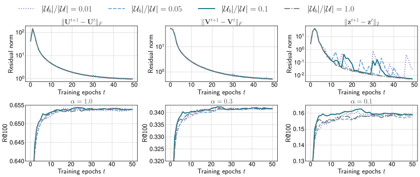
Figure 7: Convergence profile of SAFER₂ with different sampling ratio $|\mathcal{U}_{b}|/|\mathcal{U}|$ on ML-20M.

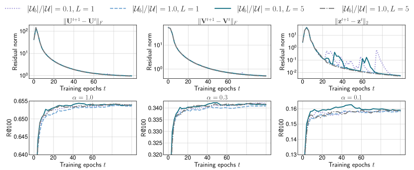
Figure 8: Convergence profile of SAFER₂ with different number of NR iterations $L$ on ML-20M.

Choice of kernels.

Various symmetric kernels can be used to instantiate SAFER₂ as discussed in Section D.3. To observe the effect of choosing kernel functions, we compare SAFER₂ with the Gaussian kernel, as examined in Section 5, and with the Epanechnikov kernel. Figure 9 demonstrates the distribution of relative ranking performance of each method compared to iALS through nested cross-validation as in Section 5. The SAFER₂ instance with the Gaussian kernel performs slightly better than the one with the Epanechnikov kernel, but the difference between them is not substantial. However, the Gaussian kernel results in stability in the $\xi$ step due to its full support property, making it easier to tune the bandwidth parameter $h$.

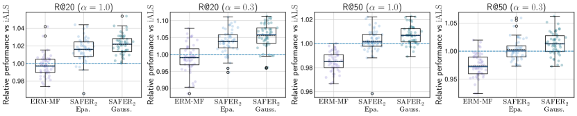
Figure 9: Distributions of relative performance vs iALS on ML-1M.

Inexact linear solvers for large embedding size.

Because SAFER₂ has quadratic/cubic runtime dependency on the embedding size $d$, we proposed a variant of SAFER₂, i.e. SAFER₂++, in Section D.4. Here, we examine the computational efficiency of SAFER₂++. To establish a baseline method for comparison, we consider another variant of SAFER₂, called SAFER₂-CG, that uses the conjugate gradient (CG) method to solve $d\times d$ linear systems. For SAFER₂-CG, we used the CG implementation in the Eigen library; the maximum number of iterations was set to five, and the error tolerance was set to $1\mathrm{e-}{4}$. We used the same hyperparameters for all models, which achieved the best ranking quality with the exact linear solver and $d=256$ for the validation split of ML-20M. In Figure 10, we present the convergence speed of SAFER₂++ on ML-20M for different values of $d$ and $|\bm{\pi}|$. For comparison, we also display the red dashed curve that corresponds to the original SAFER₂’s results, except for the case of $d=4{,}096$, where SAFER₂ did not finish in a practical time. Our results show that SAFER₂++ achieves comparable ranking quality compared to SAFER₂ for both average and semi-worst-case scenarios. Furthermore, although the convergence speed in terms of training epochs is similar for both SAFER₂ and SAFER₂++, SAFER₂++ exhibits substantially superior computational performance. When $d$ is small (e.g. $d=256$ in the second row of the figure), SAFER₂-CG (light green line) outperforms SAFER₂++ in terms of wall time. However, the performance gain of SAFER₂++ increases for larger values of $d$, such as $d=1{,}024$, $2{,}048$, or $4{,}096$, highlighting the scalability of SAFER₂++ with respect to the embedding size.

Figure 10: Effect of embedding and subspace block sizes on convergence speed of SAFER₂++.

References

- Abrarov and Quine [2011] Sanjar M Abrarov and Brendan M Quine. Efficient algorithmic implementation of the voigt/complex error function based on exponential series approximation. Applied Mathematics and Computation, 218(5):1894–1902, 2011.
- Acerbi and Tasche [2002] Carlo Acerbi and Dirk Tasche. Expected shortfall: a natural coherent alternative to value at risk. Economic notes, 31(2):379–388, 2002.
- Ahmadi-Javid [2012] Amir Ahmadi-Javid. Entropic value-at-risk: A new coherent risk measure. Journal of Optimization Theory and Applications, 155:1105–1123, 2012.
- Alexander et al. [2006] Siddharth Alexander, Thomas F Coleman, and Yuying Li. Minimizing cvar and var for a portfolio of derivatives. Journal of Banking & Finance, 30(2):583–605, 2006.
- Armijo [1966] Larry Armijo. Minimization of functions having lipschitz continuous first partial derivatives. Pacific Journal of mathematics, 16(1):1–3, 1966.
- Artzner [1997] Philippe Artzner. Thinking coherently. Risk, 10:68–71, 1997.
- Artzner et al. [1999] Philippe Artzner, Freddy Delbaen, Jean-Marc Eber, and David Heath. Coherent measures of risk. Mathematical finance, 9(3):203–228, 1999.
- Bayer et al. [2017] Immanuel Bayer, Xiangnan He, Bhargav Kanagal, and Steffen Rendle. A generic coordinate descent framework for learning from implicit feedback. In Proceedings of the 26th International Conference on World Wide Web, pages 1341–1350, 2017.
- Bertin-Mahieux et al. [2011] Thierry Bertin-Mahieux, Daniel PW Ellis, Brian Whitman, and Paul Lamere. The million song dataset. 2011.
- Boyd and Vandenberghe [2004] Stephen Boyd and Lieven Vandenberghe. Convex optimization. Cambridge university press, 2004.
- Boyd et al. [2011] Stephen Boyd, Neal Parikh, Eric Chu, Borja Peleato, Jonathan Eckstein, et al. Distributed optimization and statistical learning via the alternating direction method of multipliers. Foundations and Trends® in Machine learning, 3(1):1–122, 2011.
- Cawley and Talbot [2010] Gavin C Cawley and Nicola LC Talbot. On over-fitting in model selection and subsequent selection bias in performance evaluation. The Journal of Machine Learning Research, 11:2079–2107, 2010.
- Chernozhukov and Fernández-Val [2005] Victor Chernozhukov and Iván Fernández-Val. Subsampling inference on quantile regression processes. Sankhyā: The Indian Journal of Statistics, pages 253–276, 2005.
- Curi et al. [2020] Sebastian Curi, Kfir Y Levy, Stefanie Jegelka, and Andreas Krause. Adaptive sampling for stochastic risk-averse learning. Advances in Neural Information Processing Systems, 33:1036–1047, 2020.
- Do et al. [2021] Virginie Do, Sam Corbett-Davies, Jamal Atif, and Nicolas Usunier. Two-sided fairness in rankings via lorenz dominance. Advances in Neural Information Processing Systems, 34:8596–8608, 2021.
- Epanechnikov [1969] Vassiliy A Epanechnikov. Non-parametric estimation of a multivariate probability density. Theory of Probability & Its Applications, 14(1):153–158, 1969.
- Fernandes et al. [2021] Marcelo Fernandes, Emmanuel Guerre, and Eduardo Horta. Smoothing quantile regressions. Journal of Business & Economic Statistics, 39(1):338–357, 2021.
- Friedrichs [1944] Kurt Otto Friedrichs. The identity of weak and strong extensions of differential operators. Trans. Am. Math. Soc., 55:132–151, 1944. ISSN 0002-9947.
- Gautschi [1970] Walter Gautschi. Efficient computation of the complex error function. SIAM Journal on Numerical Analysis, 7(1):187–198, 1970.
- Gu et al. [2018] Yuwen Gu, Jun Fan, Lingchen Kong, Shiqian Ma, and Hui Zou. Admm for high-dimensional sparse penalized quantile regression. Technometrics, 60(3):319–331, 2018.
- Harper and Konstan [2015] F Maxwell Harper and Joseph A Konstan. The movielens datasets: History and context. ACM Transactions on Interactive Intelligent Systems, 2015.
- He et al. [2016] Xiangnan He, Hanwang Zhang, Min-Yen Kan, and Tat-Seng Chua. Fast matrix factorization for online recommendation with implicit feedback. In Proceedings of the 39th International ACM SIGIR conference on Research and Development in Information Retrieval, pages 549–558, 2016.
- He et al. [2021] Xuming He, Xiaoou Pan, Kean Ming Tan, and Wen-Xin Zhou. Smoothed quantile regression with large-scale inference. Journal of Econometrics, 2021.
- Horowitz [1998] Joel L Horowitz. Bootstrap methods for median regression models. Econometrica, pages 1327–1351, 1998.
- Hu et al. [2008] Yifan Hu, Yehuda Koren, and Chris Volinsky. Collaborative filtering for implicit feedback datasets. In 2008 Eighth IEEE international conference on data mining, pages 263–272. Ieee, 2008.
- Jin et al. [2021] Jikai Jin, Bohang Zhang, Haiyang Wang, and Liwei Wang. Non-convex distributionally robust optimization: Non-asymptotic analysis. Advances in Neural Information Processing Systems, 34:2771–2782, 2021.
- Jorion [2007] Philippe Jorion. Value at risk: the new benchmark for managing financial risk. The McGraw-Hill Companies, Inc., 2007.
- Koenker and Bassett Jr [1978] Roger Koenker and Gilbert Bassett Jr. Regression quantiles. Econometrica: journal of the Econometric Society, pages 33–50, 1978.
- Koenker and Hallock [2001] Roger Koenker and Kevin F Hallock. Quantile regression. Journal of economic perspectives, 15(4):143–156, 2001.
- Koenker et al. [2017] Roger Koenker, Victor Chernozhukov, Xuming He, and Limin Peng. Handbook of quantile regression. 2017.
- Koren et al. [2009] Yehuda Koren, Robert Bell, and Chris Volinsky. Matrix factorization techniques for recommender systems. Computer, 42(8):30–37, 2009.
- Krichene et al. [2018] Walid Krichene, Nicolas Mayoraz, Steffen Rendle, Li Zhang, Xinyang Yi, Lichan Hong, Ed Chi, and John Anderson. Efficient training on very large corpora via gramian estimation. 2018.
- Lan and Zhou [2018] Guanghui Lan and Yi Zhou. An optimal randomized incremental gradient method. Mathematical programming, 171:167–215, 2018.
- Lee et al. [2014] Joonseok Lee, Samy Bengio, Seungyeon Kim, Guy Lebanon, and Yoram Singer. Local collaborative ranking. In Proceedings of the 23rd international conference on World wide web, pages 85–96, 2014.
- Levy et al. [2020] Daniel Levy, Yair Carmon, John C Duchi, and Aaron Sidford. Large-scale methods for distributionally robust optimization. Advances in Neural Information Processing Systems, 33:8847–8860, 2020.
- Liang et al. [2018] Dawen Liang, Rahul G Krishnan, Matthew D Hoffman, and Tony Jebara. Variational autoencoders for collaborative filtering. In Proceedings of the 2018 world wide web conference, pages 689–698, 2018.
- Man et al. [2022] Rebeka Man, Xiaoou Pan, Kean Ming Tan, and Wen-Xin Zhou. A unified algorithm for penalized convolution smoothed quantile regression. arXiv preprint arXiv:2205.02432, 2022.
- Meng et al. [2016] Xiangrui Meng, Joseph Bradley, Burak Yavuz, Evan Sparks, Shivaram Venkataraman, Davies Liu, Jeremy Freeman, DB Tsai, Manish Amde, Sean Owen, et al. Mllib: Machine learning in apache spark. The Journal of Machine Learning Research, 17(1):1235–1241, 2016.
- Mhammedi et al. [2020] Zakaria Mhammedi, Benjamin Guedj, and Robert C Williamson. Pac-bayesian bound for the conditional value at risk. Advances in Neural Information Processing Systems, 33:17919–17930, 2020.
- Mises and Pollaczek-Geiringer [1929] RV Mises and Hilda Pollaczek-Geiringer. Praktische verfahren der gleichungsauflösung. ZAMM-Journal of Applied Mathematics and Mechanics/Zeitschrift für Angewandte Mathematik und Mechanik, 9(1):58–77, 1929.
- Park et al. [2015] Dohyung Park, Joe Neeman, Jin Zhang, Sujay Sanghavi, and Inderjit Dhillon. Preference completion: Large-scale collaborative ranking from pairwise comparisons. In International Conference on Machine Learning, pages 1907–1916. PMLR, 2015.
- Patro et al. [2020] Gourab K Patro, Arpita Biswas, Niloy Ganguly, Krishna P Gummadi, and Abhijnan Chakraborty. Fairrec: Two-sided fairness for personalized recommendations in two-sided platforms. In Proceedings of the web conference 2020, pages 1194–1204, 2020.
- Pflug [2000] Georg Ch Pflug. Some remarks on the value-at-risk and the conditional value-at-risk. Probabilistic constrained optimization: Methodology and applications, pages 272–281, 2000.
- Pilászy et al. [2010] István Pilászy, Dávid Zibriczky, and Domonkos Tikk. Fast als-based matrix factorization for explicit and implicit feedback datasets. In Proceedings of the fourth ACM conference on Recommender systems, pages 71–78, 2010.
- Poppe and Wijers [1990] Gert PM Poppe and Christianus MJ Wijers. More efficient computation of the complex error function. ACM Transactions on Mathematical Software (TOMS), 16(1):38–46, 1990.
- Qi et al. [2021] Qi Qi, Zhishuai Guo, Yi Xu, Rong Jin, and Tianbao Yang. An online method for a class of distributionally robust optimization with non-convex objectives. Advances in Neural Information Processing Systems, 34:10067–10080, 2021.
- Rahimian and Mehrotra [2019] Hamed Rahimian and Sanjay Mehrotra. Distributionally robust optimization: A review. arXiv preprint arXiv:1908.05659, 2019.
- Rendle and Freudenthaler [2014] Steffen Rendle and Christoph Freudenthaler. Improving pairwise learning for item recommendation from implicit feedback. In Proceedings of the 7th ACM international conference on Web search and data mining, pages 273–282, 2014.
- Rendle et al. [2009] Steffen Rendle, Christoph Freudenthaler, Zeno Gantner, and Lars Schmidt-Thieme. Bpr: Bayesian personalized ranking from implicit feedback. In Proceedings of the Twenty-Fifth Conference on Uncertainty in Artificial Intelligence, pages 452–461, 2009.
- Rendle et al. [2021] Steffen Rendle, Walid Krichene, Li Zhang, and Yehuda Koren. Ials++: Speeding up matrix factorization with subspace optimization. arXiv preprint arXiv:2110.14044, 2021.
- Rendle et al. [2022] Steffen Rendle, Walid Krichene, Li Zhang, and Yehuda Koren. Revisiting the performance of ials on item recommendation benchmarks. In Proceedings of the 16th ACM Conference on Recommender Systems, pages 427–435, 2022.
- Rockafellar and Uryasev [2000] R Tyrrell Rockafellar and Stanislav Uryasev. Optimization of conditional value-at-risk. Journal of risk, 2:21–42, 2000.
- Rockafellar and Uryasev [2002] R Tyrrell Rockafellar and Stanislav Uryasev. Conditional value-at-risk for general loss distributions. Journal of banking & finance, 26(7):1443–1471, 2002.
- Roosta-Khorasani and Mahoney [2019] Farbod Roosta-Khorasani and Michael W Mahoney. Sub-sampled newton methods. Mathematical Programming, 174:293–326, 2019.
- Schwartz [1951] Laurent Schwartz. Théorie des distributions. Hermann & Cie, 1951.
- Sedhain et al. [2016] Suvash Sedhain, Aditya Menon, Scott Sanner, and Darius Braziunas. On the effectiveness of linear models for one-class collaborative filtering. In Proceedings of the AAAI Conference on Artificial Intelligence, volume 30, 2016.
- Shivaswamy and Garcia-Garcia [2022] Pannaga Shivaswamy and Dario Garcia-Garcia. Adversary or friend? an adversarial approach to improving recommender systems. In Proceedings of the 16th ACM Conference on Recommender Systems, pages 369–377, 2022.
- Singh et al. [2020] Ashudeep Singh, Yoni Halpern, Nithum Thain, Konstantina Christakopoulou, E Chi, Jilin Chen, and Alex Beutel. Building healthy recommendation sequences for everyone: A safe reinforcement learning approach. In FAccTRec Workshop, 2020.
- Sobolev [1938] Sergei L. Sobolev. Sur un théorème d’analyse fonctionnelle. Recueil Mathématique (Matematicheskii Sbornik), 4(46):471–497, 1938.
- Soma and Yoshida [2020] Tasuku Soma and Yuichi Yoshida. Statistical learning with conditional value at risk. arXiv preprint arXiv:2002.05826, 2020.
- Steck [2019a] Harald Steck. Embarrassingly shallow autoencoders for sparse data. In The World Wide Web Conference, pages 3251–3257, 2019a.
- Steck [2019b] Harald Steck. Markov random fields for collaborative filtering. Advances in Neural Information Processing Systems, 32, 2019b.
- Tan et al. [2022] Kean Ming Tan, Lan Wang, Wen-Xin Zhou, et al. High-dimensional quantile regression: Convolution smoothing and concave regularization. Journal of the Royal Statistical Society Series B, 84(1):205–233, 2022.
- Tan et al. [2016] Wei Tan, Liangliang Cao, and Liana Fong. Faster and cheaper: Parallelizing large-scale matrix factorization on gpus. In Proceedings of the 25th ACM International Symposium on High-Performance Parallel and Distributed Computing, pages 219–230, 2016.
- Tseng [2001] Paul Tseng. Convergence of a block coordinate descent method for nondifferentiable minimization. Journal of optimization theory and applications, 109(3):475, 2001.
- Wang and Xiao [2017] Jialei Wang and Lin Xiao. Exploiting strong convexity from data with primal-dual first-order algorithms. In International Conference on Machine Learning, pages 3694–3702. PMLR, 2017.
- Weimer et al. [2007] Markus Weimer, Alexandros Karatzoglou, Quoc Le, and Alex Smola. Cofi rank-maximum margin matrix factorization for collaborative ranking. Advances in neural information processing systems, 20, 2007.
- Weimer et al. [2008a] Markus Weimer, Alexandros Karatzoglou, and Alex Smola. Adaptive collaborative filtering. In Proceedings of the 2008 ACM conference on Recommender systems, pages 275–282, 2008a.
- Weimer et al. [2008b] Markus Weimer, Alexandros Karatzoglou, and Alex Smola. Improving maximum margin matrix factorization. Machine Learning, 72:263–276, 2008b.
- Wen et al. [2022] Hongyi Wen, Xinyang Yi, Tiansheng Yao, Jiaxi Tang, Lichan Hong, and Ed H Chi. Distributionally-robust recommendations for improving worst-case user experience. In Proceedings of the ACM Web Conference 2022, pages 3606–3610, 2022.
- Weston et al. [2011] Jason Weston, Samy Bengio, and Nicolas Usunier. Wsabie: scaling up to large vocabulary image annotation. In Proceedings of the Twenty-Second international joint conference on Artificial Intelligence-Volume Volume Three, pages 2764–2770, 2011.
- Xu and Zhang [2009] Huifu Xu and Dali Zhang. Smooth sample average approximation of stationary points in nonsmooth stochastic optimization and applications. Mathematical programming, 119:371–401, 2009.
- Xu et al. [2016] Peng Xu, Jiyan Yang, Fred Roosta, Christopher Ré, and Michael W Mahoney. Sub-sampled newton methods with non-uniform sampling. Advances in Neural Information Processing Systems, 29, 2016.
- Zaghloul and Ali [2012] Mofreh R Zaghloul and Ahmed N Ali. Algorithm 916: computing the faddeyeva and voigt functions. ACM Transactions on Mathematical Software (TOMS), 38(2):1–22, 2012.
- Zhou et al. [2008] Yunhong Zhou, Dennis Wilkinson, Robert Schreiber, and Rong Pan. Large-scale parallel collaborative filtering for the netflix prize. In Algorithmic Aspects in Information and Management: 4th International Conference, AAIM 2008, Shanghai, China, June 23-25, 2008. Proceedings 4, pages 337–348. Springer, 2008.