Design and analysis of an exactly divergence-free hybridized discontinuous Galerkin method for incompressible flows on meshes with quadrilateral cells

Abstract

We generalise a hybridized discontinuous Galerkin method for incompressible flow problems to non-affine cells, showing that with a suitable element mapping the generalised method preserves a key invariance property that eludes most methods, namely that any irrotational component of the prescribed force is exactly balanced by the pressure gradient and does not affect the velocity field. This invariance property can be preserved in the discrete problem if the incompressibility constraint is satisfied in a sufficiently strong sense. We derive sufficient conditions to guarantee discretely divergence-free functions are exactly divergence-free and give examples of divergence-free finite elements on meshes with triangular, quadrilateral, tetrahedral, or hexahedral cells generated by a (possibly non-affine) map from their respective reference cells. In the case of quadrilateral cells, we prove an optimal error estimate for the velocity field that does not depend on the pressure approximation. Our analysis is supported by numerical results.

1 Introduction

Recently, there has been significant interest in numerical methods for incompressible flow problems that preserve a fundamental invariance property of the Stokes and Navier-Stokes equations; it can be shown using a Helmholtz decomposition that any modification to the irrotational component of the applied force is exactly balanced by the pressure gradient and does not affect the velocity field [1, 2]. Most of the classical mixed methods for incompressible flow, including the Taylor–Hood [3], MINI [4], and Crouzeix–Raviart [5] elements, do not preserve this property. This is because the divergence-free constraint is only enforced approximately, and therefore discretely divergence-free vector fields are not $L^{2}$-orthogonal to irrotational fields, resulting in poor momentum balance i.e. irrotational forces can drive spurious flow (see [1, 2] for details). These methods are not pressure robust in the sense that the pressure field can pollute the velocity approximation; error estimates for the velocity field depend on the approximation error of the pressure field scaled by the inverse of the viscosity. Hence, if the viscosity is small or if the pressure field is poorly approximated, the error in the velocity field can be large. This was demonstrated for colliding flow in a cross-shaped domain by Linke [6]. Pressure robustness can also be important to compute accurate solutions to buoyancy-driven flows and fluids in hydrostatic equilibrium [2]. A comprehensive review of the role the divergence constraint plays in discretisations of incompressible flow problems can be found in John et al. [2].

Amongst the approaches to preserve the invariance property and obtain a pressure-robust method, one is to enforce the divergence-free constraint exactly in the discrete problem [2]. There are also other benefits to using schemes that provide divergence-free velocity fields. For instance, if mass is not conserved exactly, finite element methods for the incompressible Navier–Stokes equations are typically not energy stable [7]. Moreover, a divergence-free velocity field can help avoid spurious results and instabilities when solving transport equations (such as in turbulence models [8]). Furthermore, for applications involving particle advection, such as particle-mesh methods or particle tracing, an initially uniform particle distribution does not remain uniform as time progresses unless the divergence constraint is satisfied exactly; instead, the particles clump together in a non-physical manner (see [9]).

In the case of conforming mixed methods, finite element exterior calculus [10] has proved to be a valuable tool [2] for constructing divergence-free schemes. Several methods can be viewed in this framework, including the Scott–Vogelius element [11, 12] on barycentric-refined meshes and the Guzmán–Neilan element [13, 14]. However, methods of this variety typically require either high-order polynomials, enriched spaces, special meshes, or tend to be challenging to extend to three dimensions [2, 15] due to the smoothness of the Stokes complex [2]. In general, it is difficult to balance stability and incompressibility when restricted to conforming function spaces [16].

To balance the demands of stability and incompressibility, one approach is non-conforming methods. Discontinuous Galerkin (DG) methods using only $L^{2}$-conforming approximation spaces combined with efficient (element-wise) post-processing techniques can yield divergence-free velocity approximations, see [17]. Post-processing can be avoided if the finite element velocity space is instead $H(\rm{div})$-conforming, as detailed in Cockburn et al. [18, 17] and Wang and Ye [19]. However, due to the large number of degrees of freedom introduced, DG methods are relatively expensive compared to conforming methods. This motivated the development of hybrid DG (HDG) methods which, in the spirit of hybrid mixed methods [20], introduce functions defined only over the facets of the mesh and use static condensation to eliminate the cell degrees-of-freedom. This reduces the number of globally coupled degrees of freedom considerably, especially for high-order schemes [21]. An HDG method for the Stokes equations was introduced by Cockburn and Gopalakrishnan [22] and is based on a vorticity-velocity-pressure formulation. Lehrenfeld and Schöberl [23] present an HDG method for the incompressible Navier–Stokes equations using an $H(\rm{div})$-conforming finite element space for the velocity field. In their scheme, only the tangential component of the velocity is ‘hybridized’. Rhebergen and Wells [24, 25, 26] enforce continuity of the normal component via hybridization with a simple modification of the scheme in [27]. The facet pressure space is chosen to ensure that discretely divergence-free functions are $H(\rm{div})$-conforming, otherwise pressure robustness is lost [26]. Other examples of HDG methods for the Stokes equations include [28, 29, 30].

Most of the analysis of divergence-free HDG schemes in the literature is limited to meshes made of affine cells, i.e. flat-faced simplices, parallelograms, or parallelepipeds. The method in [24] only yields a divergence-free velocity field when the mesh is made of affine simplices. It would clearly be advantageous for complex, curved geometries to preserve pressure robustness for higher-order geometric maps, and to be able to use tensor product cells for boundary layers and to apply fast integration techniques. Examples of other divergence-free methods for non-affine cells include Neilan and Otus [31], who analyse a Scott–Vogelius isoparametric finite element in two dimensions and Evans [7], who exploits the smoothness of B-splines on single-patch domains to discretise a Stokes complex, yielding an inf-sup stable and divergence-free scheme. Neilan and Sap [15] introduce a divergence-free finite element pair for the Stokes problem that is stable and conforming on shape-regular meshes made of flat-faced quadrilateral cells. Piecewise quadratic and piecewise constant polynomials are used for the velocity and pressure spaces respectively, and after post-processing, the approximate velocity and pressure fields are both second-order accurate. Methods that use $H(\mathrm{div})$-conforming elements for the velocity space, such as [17, 18, 23, 32], can also provide exactly divergence-free solutions on non-affine cells.

This work extends and generalises the HDG method from [24, 26] to non-affine and non-simplex cells whilst preserving the invariance property. Detailed analysis focuses on flat-faced quadrilateral cells, but numerical examples are presented for a range of non-affine cell types. We focus on the Stokes equations, but the results can easily be generalised to the Navier–Stokes equations. The layout of this paper is as follows: In Section 2 the proposed HDG scheme is detailed, followed in Section 3 by the conditions which, if satisfied, ensure that discretely divergence-free functions are exactly divergence-free. In Section 4, a pressure robust error estimate is derived, and in Section 5 the conditions required to apply our pressure robust error estimate are proved for a divergence-free quadrilateral element. We present numerical results to support our theoretical analysis in Section 6 and draw conclusions in Section 7.

2 Stokes flow and the hybrid discontinuous Galerkin method

Consider viscous incompressible fluid flow in a domain $\Omega\subset\mathbb{R}^{d}$, with $d\in\mathinner{\left\{2,3\right\}}$. The velocity $u\mathrel{\mathop{\ordinarycolon}}\Omega\to\mathbb{R}^{d}$ and pressure $p\mathrel{\mathop{\ordinarycolon}}\Omega\to\mathbb{R}$ satisfy the Stokes problem:

$$-\nu\Delta u+\nabla p =f \textnormal{ in }\Omega,$$ (1a)

$$\nabla\cdot u =0 \textnormal{ in }\Omega,$$ (1b)

$$u =0 \textnormal{ on }\partial\Omega,$$ (1c)

where $f\mathrel{\mathop{\ordinarycolon}}\Omega\to\mathbb{R}^{d}$ is a prescribed force and $\nu\in\mathbb{R}^{+}$ is the kinematic viscosity. The pressure is determined only up to a constant, so we seek pressure fields that satisfy the condition

$$\int_{\Omega}p\operatorname{d\!}x=0.$$ (2)

2.1 Definitions

Let $K$ denote a triangular/quadrilateral cell for $d=2$ or a tetrahedral/hexahedral cell for $d=3$ with non-zero diameter $h_{K}$. Each cell is assumed to be generated from a reference cell $\hat{K}$ via a $\mathcal{C}^{1}$-diffeomorphism $T_{K}\mathrel{\mathop{\ordinarycolon}}\hat{K}\to K$ obtained from a Lagrange geometric reference element [33]. Let the boundary of each cell be denoted by $\partial K$ with outward unit normal $n$. The domain $\Omega$ is partitioned into a mesh $\mathcal{T}_{h}=\{K\}$, and $h$ is used to denote the maximum cell diameter in the mesh. The geometric interpolation of $\Omega$, denoted $\Omega_{h}$, does not, in general, coincide exactly with $\Omega$ [33]. However, for simplicity, we assume that $\Omega_{h}=\Omega$. Let a facet in the mesh be denoted by $F$, the set of all facets by $\mathcal{F}_{h}$, and let $\Gamma_{h}\coloneqq\bigcup_{F\in\mathcal{F}_{h}}F$.

We now define the following finite element function spaces:

$$V_{h} \coloneqq\mathinner{\left\{v_{h}\in[L^{2}(\Omega_{h})]^{d};\;v_{h}|_{K}\in V_{h}(K)\;\forall K\in\mathcal{T}_{h}\right\}},$$ (3a)

$$\bar{V}_{h} \coloneqq\mathinner{\left\{\bar{v}_{h}\in[L^{2}(\Gamma_{h})]^{d};\;\bar{v}_{h}|_{F}\in\bar{V}_{h}(F)\;\forall F\in\mathcal{F}_{h},\;\bar{v}_{h}=0\textnormal{ on }\partial\Omega_{h}\right\}},$$ (3b)

$$Q_{h} \coloneqq\mathinner{\left\{q_{h}\in L^{2}(\Omega_{h});\;q_{h}|_{K}\in Q_{h}(K)\;\forall K\in\mathcal{T}_{h}\right\}},$$ (3c)

$$\bar{Q}_{h} \coloneqq\mathinner{\left\{\bar{q}_{h}\in L_{0}^{2}(\Gamma_{h});\;\bar{q}_{h}|_{F}\in\bar{Q}_{h}(F)\;\forall F\in\mathcal{F}_{h}\right\}}.$$ (3d)

The local spaces $V_{h}(K)$, $\bar{V}_{h}(F)$, $Q_{h}(K)$, and $\bar{Q}_{h}(F)$ are generated from their respective counterparts $V_{h}(\hat{K})$, $\bar{V}_{h}(\hat{F})$, $Q_{h}(\hat{K})$, and $\bar{Q}_{h}(\hat{F})$ on the reference element $\hat{K}$ or reference facet $\hat{F}$ using a linear bijective mapping (see [33, Proposition 1.61]). For instance, the space $V_{h}(K)$ is generated by

$$V_{h}(K)=\mathinner{\left\{\psi^{-1}_{K}(\hat{v});\hat{v}\in V_{h}(\hat{K})\right\}},$$ (4)

where

$$\psi_{K}\mathrel{\mathop{\ordinarycolon}}V_{h}(K)\to V_{h}(\hat{K}).$$ (5)

We leave the reference spaces and the mapping $\psi_{K}$ undefined for now. The spaces $V_{h}$ and $Q_{h}$ contain functions that are discontinuous between cells, and similarly $\bar{V}_{h}$ and $\bar{Q}_{h}$ contain functions that are discontinuous between facets. For convenience, we introduce $\bm{V}_{h}\coloneqq V_{h}\times\bar{V}_{h}$ and $\bm{Q}_{h}\coloneqq Q_{h}\times\bar{Q}_{h}$.

We follow Section 2 of [26] and introduce the extended function spaces

$$V(h) \coloneqq V_{h}+\mathinner{\left[H_{0}^{1}(\Omega_{h})\right]}^{d}\cap\mathinner{\left[H^{2}(\Omega_{h})\right]}^{d},$$ (6a)

$$\bar{V}(h) \coloneqq\bar{V}_{h}+[H_{0}^{3/2}(\Gamma_{h})]^{d},$$ (6b)

$$Q(h) \coloneqq Q_{h}+L^{2}_{0}(\Omega_{h})\cap H^{1}(\Omega_{h}),$$ (6c)

$$\bar{Q}(h) \coloneqq\bar{Q}_{h}+H_{0}^{1/2}(\Gamma_{h}),$$ (6d)

where $L^{2}_{0}(\Omega_{h})$ denotes the space of functions in $L^{2}(\Omega_{h})$ with zero mean. Further, we define the norms

$$|\!|\!|\bm{v}|\!|\!|_{v}^{2}\coloneqq\sum_{K\in\mathcal{T}_{h}}\mathinner{\!\left\lVert\nabla v\right\rVert}_{L^{2}(K)}^{2}+\sum_{K\in\mathcal{T}_{h}}\frac{\alpha}{h_{K}}\mathinner{\!\left\lVert\bar{v}-v\right\rVert}_{L^{2}(\partial K)}^{2}$$ (7)

and

$$|\!|\!|\bm{v}|\!|\!|_{v^{\prime}}^{2}\coloneqq|\!|\!|\bm{v}|\!|\!|_{v}^{2}+\sum_{K\in\mathcal{T}_{h}}\frac{h_{K}}{\alpha}\mathinner{\!\left\lVert\partial_{n}v\right\rVert}_{L^{2}(\partial K)}^{2}$$ (8)

on $V(h)\times\bar{V}(h)$, the norm

$$\mathinner{\!\left\lVert\bar{q}\right\rVert}_{p}^{2}\coloneqq\sum_{K\in\mathcal{T}_{h}}h_{K}\mathinner{\!\left\lVert\bar{q}\right\rVert}_{L^{2}(\partial K)}^{2}$$ (9)

on $\bar{Q}(h)$, and the norm

$$|\!|\!|\bm{q}|\!|\!|_{p}^{2}\coloneqq\mathinner{\!\left\lVert q\right\rVert}_{L^{2}(\Omega_{h})}^{2}+\mathinner{\!\left\lVert\bar{q}\right\rVert}_{p}^{2}$$ (10)

on $Q(h)\times\bar{Q}(h)$.

2.2 Discrete problem

The discrete problem consists of the following: given $f\in\mathinner{\left[L^{2}(\Omega_{h})\right]}^{d}$, find $(\bm{u}_{h},\bm{p}_{h})\in\bm{V}_{h}\times\bm{Q}_{h}$ such that

$$a_{h}(\bm{u}_{h},\bm{v}_{h})+b_{h}(v_{h},\bm{p}_{h}) =f_{h}(v_{h})\quad \forall\bm{v}_{h}\in\bm{V}_{h},$$ (11a)

$$b_{h}(u_{h},\bm{q}_{h}) =0\quad \forall\bm{q}_{h}\in\bm{Q}_{h},$$ (11b)

where the bilinear forms are given by

$$\begin{split}a_{h}(\bm{u}_{h},\bm{v}_{h})\coloneqq&\sum_{K\in\mathcal{T}_{h}}\int_{K}\nu\nabla u_{h}\mathrel{\mathop{\ordinarycolon}}\nabla v_{h}\operatorname{d\!}x\\ &-\sum_{K\in\mathcal{T}_{h}}\int_{\partial K}\nu\mathinner{\left((u_{h}-\bar{u}_{h})\cdot\partial_{n}v_{h}+\partial_{n}u_{h}\cdot(v_{h}-\bar{v}_{h})\right)}\operatorname{d\!}s\\ &+\sum_{K\in\mathcal{T}_{h}}\int_{\partial K}\nu\frac{\alpha}{h_{K}}(u_{h}-\bar{u}_{h})\cdot(v_{h}-\bar{v}_{h})\operatorname{d\!}s\end{split}$$ (12)

and

$$b_{h}(v_{h},\bm{p}_{h})\coloneqq-\sum_{K\in\mathcal{T}_{h}}\int_{K}p_{h}\nabla\cdot v_{h}\operatorname{d\!}x+\sum_{K\in\mathcal{T}_{h}}\int_{\partial K}v_{h}\cdot n\bar{p}_{h}\operatorname{d\!}s,$$ (13)

where $\alpha>0$ is a penalty parameter. The linear form is defined as

$$f_{h}(v_{h})\coloneqq\int_{\Omega_{h}}f\cdot v_{h}\operatorname{d\!}x.$$ (14)

The above discrete problem is derived by posing mass and momentum balances cell-wise, subject to ‘boundary conditions’ provided by the facet fields. Equations for the facet fields are obtained by enforcing (weak) continuity of numerical fluxes across facets [27]. Critically, the numerical fluxes depend only on quantities that are either local to a particular cell or that live on the facet shared by the cell and its neighbour. The cell fields communicate only via the facet fields, meaning static condensation can be used to eliminate the cell unknowns from the global system of equations.

3 The invariance property and incompressibility

There exists a fundamental invariance property of incompressible flow; the irrotational component of the prescribed force $f\in[L^{2}(\Omega)]^{d}$ affects only the pressure field, not the velocity field. If $(u,p)$ solves the Stokes problem 1, adding $\nabla\psi$ to the force $f$, where $\psi\in H^{1}(\Omega)\setminus\mathbb{R}$, changes the solution to $(u,p+\psi)$ [2]. Pressure robust methods preserve this property in the sense that if $(u_{h},p_{h})$ solves the discrete problem, then the above modification to the applied force changes the discrete solution to $(u_{h},p_{h}+\Pi_{Q_{h}}\psi)$, where $\Pi_{Q_{h}}$ is the $L^{2}$-projection onto $Q_{h}$ (see [2, Lemma 4.6]). In this sense, contributions to the prescribed force that only affect the pressure in the continuous problem also only affect the pressure in the discrete problem [2]. As shown by John et al. [2], for pressure robust methods the a priori error estimate for the velocity field does not depend on the pressure approximation, in contrast to methods where the velocity error estimate depends on the error in the pressure scaled by the inverse of the viscosity. Pressure-robust methods are desirable since the pressure field cannot pollute the approximation of the velocity field.

Preservation of the invariance property and pressure robustness are intimately related to the sense in which the incompressibility constraint is satisfied in the discrete problem. Equation 11b constrains the discrete velocity solution to lie in the space of discretely divergence-free functions,

$$X_{h}\coloneqq\mathinner{\left\{v_{h}\in V_{h};\;b_{h}(v_{h},\bm{q}_{h})=0\quad\forall\bm{q}_{h}\in\bm{Q}_{h}\right\}}.$$ (15)

It is possible to construct pressure-robust methods by ensuring that discretely divergence-free functions are also weakly divergence-free, the meaning of which we now make precise.

Definition 1 (Weakly divergence-free).

A function $v\in H(\rm{div};\Omega)$ is weakly divergence-free (written in short as $\nabla\cdot v=0$) if

$$\int_{\Omega}v\cdot\nabla\psi\operatorname{d\!}x=0\quad\forall\psi\in C_{0}^{\infty}(\Omega).$$ (16)

Definition 1 implies $v$ is divergence-free in the classical sense in regular regions and has continuous normal components at their interfaces [34]. We denote the space of weakly divergence-free functions by

$$X\coloneqq\left\{v\in H(\textnormal{div};\Omega);\nabla\cdot v=0\right\},$$ (17)

where $\nabla\cdot v=0$ is understood in the sense of Definition 1. For numerous common finite elements for incompressible flows, the space of discretely divergence-free functions is not a subset of the space of weakly divergence-free functions. In some cases, e.g. Taylor–Hood elements, the pressure space is not rich enough to enforce the divergence constraint exactly. In other cases, e.g. standard discontinuous Galerkin methods, discretely divergence-free functions may have discontinuous normal components.

For the discrete problem in Section 2.2, sufficient conditions for the inclusion $X_{h}\subset X$ to be satisfied are:

1. the property $v_{h}|_{F}\cdot n\in\bar{Q}_{h}(F)\ \forall v_{h}\in V_{h}(K)$, which ensures elements of $X_{h}$ have continuous normal components across facets; and

2. the nesting $\nabla\cdot V_{h}(K)\subseteq Q_{h}(K)$, which ensures that elements of $X_{h}$ are divergence-free on cell interiors.

For simplex cells, Lagrange elements have these sufficient properties provided that the geometric map is affine, see [24]. However, this is not the case when the geometric map is non-affine or for non-simplex Lagrange elements. Indeed, in both of these cases, simple calculations and numerical experiments confirm that the inclusion $X_{h}\subset X$ does not hold. A similar issue affects the conforming isoparametric Scott–Vogelius element, see [31].

We now demonstrate that, if functions are transformed between the reference and physical elements in an appropriate manner, it is possible to state sufficient conditions for the inclusion $X_{h}\subset X$ to hold in terms of the relationships between the reference finite element function spaces instead of the physical finite element function spaces, and therefore independently of the geometric map $T_{K}$. Key to this is the contravariant Piola transform defined by [33, eq. (1.81)]

$$\psi_{K}(v)\coloneqq\det(J_{K})J_{K}^{-1}(v\circ T_{K}),$$ (18)

where $J_{K}$ is the Jacobian matrix of $T_{K}$. For an illustration of how $\psi_{K}$ transforms vector fields, we refer the reader to [35]. The contravariant Piola transform preserves divergence in the sense that [36, p. 2430]

$$\int_{K}\nabla\cdot vq\operatorname{d\!}x=\int_{\hat{K}}\hat{\nabla}\cdot\hat{v}\hat{q}\operatorname{d\!}\hat{x}$$ (19)

and normal components in the sense that [36, p. 2430]

$$\int_{\partial K}v\cdot nq\operatorname{d\!}s=\int_{\partial\hat{K}}\hat{v}\cdot\hat{n}\hat{q}\operatorname{d\!}\hat{s},$$ (20)

where $\hat{v}\mathrel{\mathop{\ordinarycolon}}\hat{K}\to\mathbb{R}^{d}$, $v=\psi_{K}^{-1}(\hat{v})\mathrel{\mathop{\ordinarycolon}}K\to\mathbb{R}^{d}$, $\hat{q}\mathrel{\mathop{\ordinarycolon}}\hat{K}\to\mathbb{R}$, $q=\hat{q}\circ T_{K}^{-1}\mathrel{\mathop{\ordinarycolon}}K\to\mathbb{R}$, and $\hat{n}$ denotes the unit outward normal to $\partial\hat{K}$. Using the contravariant Piola transform to construct $V_{h}$, it is possible to write sufficient conditions to ensure $X_{h}\subset X$ that are independent of the geometric map $T_{K}$; we show this in the following lemmas.

Lemma 1.

Let $V_{h}(\hat{K})\subset H(\textnormal{div};\hat{K})$ and $\bar{Q}_{h}(\hat{F})$ be finite dimensional polynomial spaces chosen such that

$$\bar{Q}_{h}(\hat{F})\supseteq\mathinner{\left\{\hat{v}_{h}|_{\hat{F}}\cdot\hat{n};\hat{v}_{h}\in V_{h}(\hat{K})\right\}}.$$ (21)

Also let $V_{h}(K)$ be generated by Eq. 4 with $\psi_{K}$ taken as the contravariant Piola transform (Eq. 18) and generate $\bar{Q}_{h}(F)$ similarly but using the composition $\psi_{F}(\bar{q}_{h})\coloneqq\bar{q}_{h}\circ T_{K}|_{\hat{F}}$. Then, discretely divergence-free functions have continuous normal components (i.e. $X_{h}\subset H(\textnormal{div};\Omega_{h})$).

Proof.

Let $v_{h}\in X_{h}$, giving $b_{h}(v_{h},\bm{q}_{h})=0\;\forall\bm{q}_{h}\in\bm{Q}_{h}$ by definition. Set $\bm{q}_{h}=(0,\bar{q}_{h})$ on a single interior facet $F$ and $\bm{q}_{h}=(0,0)$ elsewhere. The result then follows from transforming to the reference element and using the fact that the contravariant Piola transform preserves normal traces. ∎

Remark 1.

Since we consider the Stokes problem subject to the homogeneous Dirichlet boundary condition given in Eq. 1c, provided that the requirements of Lemma 1 hold, we in fact have that $X_{h}\subset H_{0}(\textnormal{div};\Omega_{h})$, where

$$H_{0}(\textnormal{div};\Omega_{h})\coloneqq\left\{v\in H(\textnormal{div};\Omega_{h});\;v\cdot n|_{\partial\Omega_{h}}=0\right\}.$$ (22)

In other words, the normal component of any discretely divergence-free function is exactly zero on the domain boundary. This can be seen by considering a facet on the domain boundary and applying a similar argument to the proof of Lemma 1.

Lemma 2.

If the conditions of Lemma 1 are satisfied and if $V_{h}(\hat{K})$ and $Q_{h}(\hat{K})$ are chosen such that

$$\hat{\nabla}\cdot V_{h}(\hat{K})\subseteq Q_{h}(\hat{K}),$$ (23)

then discretely divergence-free functions are weakly divergence-free (i.e. $X_{h}\subset X$).

Proof.

Let $v_{h}\in X_{h}$, thus $b_{h}(v_{h},\bm{q}_{h})=0\;\forall\bm{q}_{h}\in\bm{Q}_{h}$ by definition. Set $\bm{q}_{h}=(q_{h},0)$ on an element $K$ and $\bm{q}_{h}=(0,0)$ elsewhere. The result then follows from transforming to the reference element and using the fact that the contravariant Piola transform preserves divergence. ∎

Using these results, we now give some examples of finite elements for which discretely divergence-free functions are weakly divergence-free, which will be referred to as “divergence-free elements”. Let $\mathbb{P}_{k}$ denote the space of polynomials of degree at most $k$. If the mesh is made of (possibly curved) simplex cells, then choosing

$$V_{h}(\hat{K})\coloneqq[\mathbb{P}_{k}(\hat{K})]^{d},\quad\bar{V}_{h}(\hat{F})\coloneqq[\mathbb{P}_{k}(\hat{F})]^{d},\quad Q_{h}(\hat{K})\coloneqq\mathbb{P}_{k-1}(\hat{K}),\quad\textnormal{and}\quad\bar{Q}_{h}(\hat{F})\coloneqq\mathbb{P}_{k}(\hat{F})$$

implies that discretely divergence-free functions are exactly divergence-free. Indeed, for any $\hat{v}_{h}\in[\mathbb{P}_{k}(\hat{K})]^{d}$ we have $\hat{v}_{h}|_{\hat{F}}\cdot\hat{n}\in\mathbb{P}_{k}(\hat{F})$ and $\nabla\cdot[\mathbb{P}_{k}(\hat{K})]^{d}=\mathbb{P}_{k-1}(\hat{K})$; thus, Lemmas 1 and 2 can be applied.

In the case of (possibly curved) quadrilateral and hexahedral cells, following an approach similar to the divergence-conforming methods [18, 23] we choose

$$V_{h}(\hat{K})\coloneqq\mathbb{RT}_{k}(\hat{K}),\quad\bar{V}_{h}(\hat{F})\coloneqq[\mathbb{Q}_{k}(\hat{F})]^{d},\quad Q_{h}(\hat{K})\coloneqq\mathbb{Q}_{k}(\hat{K}),\quad\textnormal{and}\quad\bar{Q}_{h}(\hat{F})\coloneqq\mathbb{Q}_{k}(\hat{F}),$$

where $\mathbb{RT}_{k}$ denotes the Raviart–Thomas [37] space of index $k$, and $\mathbb{Q}_{k}$ denotes the space of polynomials of degree at most $k$ in each variable. These spaces have the property that for any $\hat{v}_{h}\in\mathbb{RT}_{k}(\hat{K})$, we have $\hat{v}_{h}|_{\hat{F}}\cdot\hat{n}\in\mathbb{Q}_{k}(\hat{F})$ and $\nabla\cdot\mathbb{RT}_{k}(\hat{K})=\mathbb{Q}_{k}(\hat{K})$ [20, p. 97]. Another divergence-free choice is to instead take

$$V_{h}(\hat{K})\coloneqq\mathbb{BDM}_{k}(\hat{K})\quad\textnormal{and}\quad Q_{h}(\hat{K})\coloneqq\mathbb{Q}_{k-1}(\hat{K})$$

with the same facet spaces, where $\mathbb{BDM}_{k}$ is the Brezzi–Douglas–Marini [38] space of index $k$.

For the seemingly natural choice of

$$V_{h}(\hat{K})\coloneqq[\mathbb{Q}_{k}(\hat{K})]^{d},\quad\bar{V}_{h}(\hat{F})\coloneqq[\mathbb{Q}_{k}(\hat{F})]^{d},\quad Q_{h}(\hat{K})\coloneqq\mathbb{Q}_{k-1}(\hat{K}),\quad\textnormal{and}\quad\bar{Q}_{h}(\hat{F})\coloneqq\mathbb{Q}_{k}(\hat{F}),$$

we have $\nabla\cdot[\mathbb{Q}_{k}(\hat{K})]^{d}\nsubseteq\mathbb{Q}_{k-1}(\hat{K})$ and it is possible to find elements of $X_{h}$ that are not elements of $X$. As a simple example, take $k=1$ and consider the function $v_{h}\coloneqq\psi_{K}^{-1}((\hat{x}_{0}+c\hat{x}_{0}\hat{x}_{1},0))\in V_{h}(K)$, where $c\coloneqq-|\hat{K}|/\int_{\hat{K}}\hat{x}_{1}\operatorname{d\!}\hat{x}$ is a constant. It is straightforward to verify that $v_{h}$ satisfies $\int_{K}q_{h}\nabla\cdot v_{h}\operatorname{d\!}x=0$ for all $q_{h}\in Q_{h}(K)$ and thus is discretely divergence-free, however, it is clearly not weakly divergence-free.

4 Pressure-robust error estimate

In this section, we use standard arguments to derive a pressure-robust error estimate for the method described in Section 2.2. We begin by stating some assumptions to ensure that the discrete problem is well-posed and that $\bm{V}_{h}$ and $\bm{Q}_{h}$ have suitable approximation properties. The validity of these assumptions is discussed in Remark 2 below.

Assumption 1 (Discretely divergence-free functions are exactly divergence-free).

Assume that $X_{h}\subset X$ (see Section 3).

Assumption 2 (Consistency).

If $(u,p)\in([H_{0}^{1}(\Omega)]^{d}\cap[H^{2}(\Omega)]^{d})\times(L_{0}^{2}(\Omega)\cap H^{1}(\Omega))$ solves the Stokes problem 1, then letting $\bm{u}\coloneqq(u,u|_{\Gamma_{h}})$ and $\bm{p}\coloneqq(p,p|_{\Gamma_{h}})$, it holds that

$$a_{h}(\bm{u},\bm{v}_{h})+b_{h}(v_{h},\bm{p}) =f_{h}(v_{h})\quad \forall\bm{v}_{h}\in\bm{V}_{h},$$ (24a)

$$b_{h}(u,\bm{q}_{h}) =0\quad \forall\bm{q}_{h}\in\bm{Q}_{h}.$$ (24b)

Assumption 3 (Norm equivalence on $\bm{V}_{h}$).

There exists a constant $c$, independent of $h$, such that for all $\bm{v}_{h}\in\bm{V}_{h}$

$$|\!|\!|\bm{v}_{h}|\!|\!|_{v}\leq|\!|\!|\bm{v}_{h}|\!|\!|_{v^{\prime}}\leq c|\!|\!|\bm{v}_{h}|\!|\!|_{v}.$$ (25)

In other words, the norms $|\!|\!|\cdot|\!|\!|_{v}$ and $|\!|\!|\cdot|\!|\!|_{v^{\prime}}$ are equivalent on $\bm{V}_{h}$.

Assumption 4 (Stability of $a_{h}$).

There exists a $\beta_{v}>0$ that is independent of $h$ and a constant $\alpha_{0}>0$ such that for $\alpha>\alpha_{0}$

$$a_{h}(\bm{v}_{h},\bm{v}_{h})\geq\nu\beta_{v}|\!|\!|\bm{v}_{h}|\!|\!|_{v}^{2}\quad\forall\bm{v}_{h}\in\bm{V}_{h}.$$ (26)

Assumption 5 (Boundedness of $a_{h}$).

There exists a constant $C_{a}>0$, independent of $h$, such that $\forall\bm{u}\in V(h)\times\bar{V}(h)$ and $\forall\bm{v}_{h}\in\bm{V}_{h}$

$$|a_{h}(\bm{u},\bm{v}_{h})|\leq\nu C_{a}|\!|\!|\bm{u}|\!|\!|_{v^{\prime}}|\!|\!|\bm{v}_{h}|\!|\!|_{v}.$$ (27)

Assumption 6 (Stability of $b_{h}$).

There exists a constant $\beta_{p}>0$, independent of $h$, such that

$$\inf_{\bm{q}_{h}\in\bm{Q}_{h}}\sup_{\bm{v}_{h}\in\bm{V}_{h}}\frac{b_{h}(v_{h},\bm{q}_{h})}{|\!|\!|\bm{v}_{h}|\!|\!|_{v}|\!|\!|\bm{q}_{h}|\!|\!|_{p}}\geq\beta_{p}.$$ (28)

Assumption 7 (Boundedness of $b_{h}$).

There exists a constant $C_{b}>0$ that is independent of $h$ such that $\forall\bm{v}_{h}\in\bm{V}_{h}$ and $\forall\bm{p}\in Q(h)\times\bar{Q}(h)$

$$|b_{h}(v_{h},\bm{p})|\leq C_{b}|\!|\!|\bm{v}_{h}|\!|\!|_{v}|\!|\!|\bm{p}|\!|\!|_{p}.$$ (29)

Assumption 8 (Approximation properties of $\bm{V}_{h}$ and $\bm{Q}_{h}$).

For any $(v,q)\in[H_{0}^{k+1}(\Omega)]^{d}\times H^{k}(\Omega)$ with $k\geq 1$, letting $\bm{v}\coloneqq(v,v|_{\Gamma_{h}})$ and $\bm{q}\coloneqq(q,q|_{\Gamma_{h}})$, there holds

$$\inf_{\bm{v}_{h}\in\bm{V}_{h}}|\!|\!|\bm{v}-\bm{v}_{h}|\!|\!|_{v^{\prime}}\leq ch^{k}\mathinner{\!\left\lVert v\right\rVert}_{H^{k+1}(\Omega)},$$ (30)

and

$$\inf_{\bm{q}_{h}\in\bm{Q}_{h}}|\!|\!|\bm{q}-\bm{q}_{h}|\!|\!|_{p}\leq ch^{k}\mathinner{\!\left\lVert q\right\rVert}_{H^{k}(\Omega)},$$ (31)

where $c$ is a constant independent of $h$.

We are now able to derive the following pressure robust error estimate.

Theorem 1 (Error estimate).

Let $(u,p)\in[H_{0}^{k+1}(\Omega)]^{d}\times H^{k}(\Omega)$ solve the Stokes system given by Eq. 1 with $k\geq 1$, and set $\bm{u}\coloneqq(u,u|_{\Gamma_{h}})$ and $\bm{p}\coloneqq(p,p|_{\Gamma_{h}})$. Let Assumptions 1 to 8 be satisfied and let $(\bm{u}_{h},\bm{p}_{h})\in\bm{V}_{h}\times\bm{Q}_{h}$ solve the discrete problem given by Eq. 11. Then, we have

$$|\!|\!|\bm{u}-\bm{u}_{h}|\!|\!|_{v}\leq ch^{k}\mathinner{\!\left\lVert v\right\rVert}_{H^{k+1}(\Omega)},$$ (32)

and

$$\mathinner{\!\left\lVert p-p_{h}\right\rVert}_{L^{2}(\Omega)}\leq ch^{k}\left(\mathinner{\!\left\lVert p\right\rVert}_{H^{k}(\Omega)}+\nu\mathinner{\!\left\lVert u\right\rVert}_{H^{k+1}(\Omega)}\right),$$ (33)

where $c>0$ is independent of $h$. In addition, if some restrictions are placed on the shape of $\Omega$ [25] such that the regularity condition

$$\nu\mathinner{\!\left\lVert u\right\rVert}_{H^{2}(\Omega)}+\mathinner{\!\left\lVert p\right\rVert}_{H^{1}(\Omega)}\leq c_{r}\mathinner{\!\left\lVert f\right\rVert}_{L^{2}(\Omega)},$$ (34)

holds for some constant $c_{r}$, then

$$\mathinner{\!\left\lVert u-u_{h}\right\rVert}_{L^{2}(\Omega)}\leq ch^{k+1}\mathinner{\!\left\lVert u\right\rVert}_{H^{k+1}(\Omega)}.$$ (35)

Proof.

The velocity and pressure error estimates follow from Assumptions 1 to 8 using standard arguments, so we omit the details. The error estimate in the $L^{2}(\Omega)$-norm can be obtained using the Aubin–Nitsche duality method. ∎

Remark 2 (Validity of assumptions).

When the mesh cells are generated from an affine map from the reference simplex, square, or cube, e.g. flat sided triangles, tetrahedra, parallelograms, and parallelepipeds, it is straightforward to verify that the assumptions hold for all of the divergence-free elements discussed in Section 3 using an approach similar to [26, Section 2]. We therefore omit the proofs in this work. When the maps are non-affine, it is more complicated to verify that the assumptions hold. The main difficulty is the loss of approximation accuracy of standard $H(\textrm{div})$-conforming elements on general meshes. Arnold et al. [36] prove necessary and sufficient conditions for $H(\textrm{div})$-conforming elements to achieve optimal order approximation in $L^{2}$ on cells generated from a bilinear isomorphism of the square (i.e. flat-faced quadrilaterals). These conditions are satisfied by Raviart-Thomas elements but not by Brezzi–Douglas–Marini elements. The order of approximation in the $L^{2}$-norm of $\mathbb{BDM}_{k}$ degrades from $k+1$ in the affine case to $\lfloor(k+1)/2\rfloor$ in the bilinear case. The situation is more complicated in three dimensions; Falk et al. [39] show that standard $H(\textrm{div})$-conforming elements do not achieve optimal order approximation on cells generated by a trilinear isomorphism of the cube. In Section 5, we restrict the analysis to the divergence-free Raviart–Thomas element from Section 3 on flat-faced quadrilateral cells, leaving more complex cell types and geometric maps to be investigated as further work.

5 Proof of assumptions for flat-faced quadrilateral cells

Up to this point, the presentation has been quite general; Lemmas 1 and 2 give sufficient conditions for discretely divergence-free functions to be exactly divergence-free regardless of whether the geometric map $T_{K}$ is affine or not, we have given examples of divergence-free elements on simplices, quadrilateral, and hexahedral cells in Section 3, and the pressure robust error estimate derived in Section 4 applies to any divergence-free element that satisfies Assumptions 2 to 8. We now focus specifically on the divergence-free Raviart–Thomas element discussed in Section 3 on families of shape-regular meshes of flat-faced quadrilateral cells, for which we prove Assumptions 2 to 8. Recall that Assumption 1 was proved for the Raviart–Thomas element in Section 3.

Let the mesh be made of flat-faced quadrilateral cells which are the image of the reference square under a bilinear diffeomorphism, i.e. $T_{K}\in[\mathbb{Q}_{1}(\hat{K})]^{2}$ [40]. Recall that $J_{K}$ is the Jacobian matrix of $T_{K}$. We assume each cell is convex, which implies that [33, Lemma 1.119]

$$\begin{split}\mathinner{\!\left\lVert\det(J_{K})\right\rVert}_{L^{\infty}(\hat{K})}&\leq ch_{K}^{2},\quad\mathinner{\!\left\lVert\det(J_{K}^{-1})\right\rVert}_{L^{\infty}(K)}\leq c\frac{1}{\rho_{K}^{2}},\quad\\ \mathinner{\!\left\lVert J_{K}\right\rVert}_{L^{\infty}(\hat{K})}&\leq ch_{K},\quad\mathinner{\!\left\lVert J_{K}^{-1}\right\rVert}_{L^{\infty}(K)}\leq c\frac{h_{K}}{\rho_{K}^{2}},\end{split}$$ (36)

where $\rho_{K}\coloneqq\min_{i\in\{1\mathrel{\mathop{\ordinarycolon}}4\}}\rho_{i}$, $\rho_{i}$ is the diameter of the largest circle that can be inscribed into the triangle formed by the three vertices $(a_{j})_{j\neq i}$ of $K$. Let the family of meshes $\left\{\mathcal{T}_{h}\right\}_{h>0}$ be shape-regular in the sense that there exists a $\sigma_{0}$ such that for all $h$ and for all $K\in\mathcal{T}_{h}$, $\sigma_{K}\coloneqq h_{K}/\rho_{K}\leq\sigma_{0}$ [33]. As such, the analysis does not hold for, for example, highly stretched (high aspect ratio) cells in the mesh. We refer to [41] for more on the theoretical aspects of such anisotropic cells.

5.1 Some useful results on quadrilateral cells

To prove Assumptions 2 to 8, we require the following results.

Lemma 3 (Broken Poincaré inequality).

For all $\bm{v}_{h}\in\bm{V}_{h}$, there is a constant $c>0$, independent of $h$, such that

$$\mathinner{\!\left\lVert v_{h}\right\rVert}_{L^{2}(\Omega)}\leq c|\!|\!|\bm{v}_{h}|\!|\!|_{v}.$$ (37)

Proof.

A simple consequence of [42, Eq. (4.21)]. ∎

Lemma 4 (Inverse inequality).

For all $K\in\mathcal{T}_{h}$ and $l\in\{1,2\}$, there exists a constant $c>0$, independent of $h$, such that $\forall v_{h}\in V_{h}$

$$\mathinner{\!\left\lVert v_{h}\right\rVert}_{H^{l}(K)}\leq ch_{K}^{-1}\mathinner{\!\left\lVert v_{h}\right\rVert}_{H^{l-1}(K)}.$$ (38)

Proof.

The result is stated for flat-faced quadrilateral cells in Lemma 3.6 of [43] and proved for hexahedral cells in Lemma 3.5 of [44]. ∎

Lemma 5 (Discrete Trace Inequality).

For all $K\in\mathcal{T}_{h}$, there exists a constant $c>0$, independent of $h$, such that $\forall v_{h}\in V_{h}$

$$\mathinner{\!\left\lVert v_{h}\right\rVert}_{L^{2}(\partial K)}\leq ch_{K}^{-\frac{1}{2}}\mathinner{\!\left\lVert v_{h}\right\rVert}_{L^{2}(K)}$$ (39)

and

$$\mathinner{\!\left\lVert\partial_{n}v_{h}\right\rVert}_{L^{2}(\partial K)}\leq ch_{K}^{-\frac{1}{2}}\mathinner{\!\left\lVert v_{h}\right\rVert}_{H^{1}(K)}.$$ (40)

Proof.

The results follow from the continuous trace inequality [45, Theorem 3.2]

$$\mathinner{\!\left\lVert v\right\rVert}_{L^{2}(\partial K)}^{2}\leq c\left(h_{K}^{-1}\mathinner{\!\left\lVert v\right\rVert}_{L^{2}(K)}^{2}+h_{K}\mathinner{\!\left\lvert v\right\rvert}_{H^{1}(K)}^{2}\right),$$ (41)

which holds for all $v\in H^{1}(K)$, and Lemma 4 (see [7, Lemma 5.6.2]). ∎

We now introduce the space

$$Y_{h}\coloneqq\left\{v_{h}\in V_{h};\;\llbracket v_{h}\cdot n\rrbracket=0\textnormal{ on }F\;\forall F\in\mathcal{F}_{h}^{i}\right\},$$ (42)

where $\mathcal{F}_{h}^{i}$ denotes the set of interior facets of the mesh and $\llbracket v_{h}\cdot n\rrbracket\coloneqq v|_{K_{0}}\cdot n|_{K_{0}}+v|_{K_{1}}\cdot n|_{K_{1}}$, where $K_{0}$ and $K_{1}$ are the cells sharing $F\in\mathcal{F}_{h}^{i}$. $Y_{h}$ consists of functions in $V_{h}$ with continuous normal components across element boundaries. Let $\mathcal{I}_{h}^{RT}\mathrel{\mathop{\ordinarycolon}}[H_{0}^{1}(\Omega)]^{2}\to Y_{h}$ be the global Raviart–Thomas interpolation operator. We then have the following lemma.

Lemma 6.

Let $v\in[H^{l}(K)]^{d}$ and $m\in\{0\mathrel{\mathop{\ordinarycolon}}1\}$. If (i) $l=1$ or (ii) $v$ is divergence-free and $l\in\{1\mathrel{\mathop{\ordinarycolon}}k+1\}$, then there exists a constant $c$, independent of $h_{K}$, such that for all $K\in\mathcal{T}_{h}$

$$\mathinner{\!\left\lvert v-\mathcal{I}_{h}^{RT}v\right\rvert}_{H^{m}(K)}\leq ch_{K}^{l-m}\mathinner{\!\left\lVert v\right\rVert}_{H^{l}(K)}.$$ (43)

Proof.

The result follows from [46, Eq. (3.66) and Remark 3.5]. ∎

For a flat-faced quadrilateral cell $K$, let

$$\mathcal{R}_{k}(\partial K)\coloneqq\left\{\bar{q}_{h};\;\bar{q}_{h}\in L^{2}(\partial K),\bar{q}_{h}|_{F}\in\mathbb{Q}_{k}(F)\;\forall F\in\mathcal{F}_{K}\right\},$$ (44)

where $\mathcal{F}_{K}$ denotes the set of facets belonging to $K$. We then have the following.

Lemma 7 (Lifting operator).

For flat-faced quadrilateral cells, there exists a linear lifting operator $L\mathrel{\mathop{\ordinarycolon}}\mathcal{R}_{k}(\partial K)\to V_{h}(K)$, such that

$$(L\bar{q}_{h})\cdot n=\bar{q}_{h}\quad\textnormal{and}\quad\mathinner{\!\left\lVert L\bar{q}_{h}\right\rVert}_{L^{2}(K)}\leq ch_{K}^{\frac{1}{2}}\mathinner{\!\left\lVert\bar{q}_{h}\right\rVert}_{L^{2}(\partial K)}$$ (45)

for all $\bar{q}_{h}\in\mathcal{R}_{k}(\partial K)$.

Proof.

The proof is a simple modification of Proposition 2.4 of [47]. We begin by defining the lifting of $\bar{q}_{h}\in\mathcal{R}_{k}(\partial K)$ as the unique function $v_{h}\coloneqq L\bar{q}_{h}\in V_{h}(K)$ satisfying

$$\int_{\hat{K}}\hat{v}_{h}\cdot\hat{w}_{h}\operatorname{d\!}\hat{x}=0\quad\forall\hat{w}_{h}\in\mathbb{Q}_{k-1,k}(\hat{K})\times\mathbb{Q}_{k,k-1}(\hat{K})$$ (46)

and

$$\int_{\partial\hat{K}}\hat{v}_{h}\cdot\hat{n}\hat{r}_{h}\operatorname{d\!}\hat{s}=\int_{\partial\hat{K}}\check{\bar{q}}_{h}\hat{r}_{h}\operatorname{d\!}\hat{s}\quad\forall\hat{r}_{h}\in\mathcal{R}_{k}(\partial\hat{K}),$$ (47)

where $\hat{v}_{h}\coloneqq\psi_{K}(v_{h})$ and $\check{\bar{q}}_{h}\coloneqq|\det(J_{K})|\mathinner{\!\left\lVert J_{K}^{-T}\hat{n}\right\rVert}_{\ell^{2}}\bar{q}_{h}\circ T_{K}$; the motivation for the latter definition will become evident shortly. Now, for any $\hat{r}_{h}\in\mathcal{R}_{k}(\partial\hat{K})$ the function $r_{h}\coloneqq\hat{r}_{h}\circ T_{K}^{-1}$ is an element of $\mathcal{R}_{k}(\partial K)$ because, for flat-faced quadrilaterals, the geometric mapping $T_{K}$ is affine when restricted to the cell’s facets [43, p. 172]. In addition, we have

$$\begin{split}\int_{\partial K}v_{h}\cdot nr_{h}\operatorname{d\!}s=\int_{\partial\hat{K}}\hat{v}_{h}\cdot\hat{n}\hat{r}_{h}\operatorname{d\!}\hat{s}=\int_{\partial\hat{K}}\check{\bar{q}}_{h}\hat{r}_{h}\operatorname{d\!}\hat{s}=\int_{\partial K}\bar{q}_{h}r_{h}\operatorname{d\!}s,\end{split}$$ (48)

where the first equality follows from Eq. 20, the second from Eq. 47, and the third from the fact that the measures $\operatorname{d\!}s$ and $\operatorname{d\!}\hat{s}$ are related by [40, eq. (9.12a)]

$$\operatorname{d\!}s=|\det(J_{K})|\mathinner{\!\left\lVert J_{K}^{-T}\hat{n}\right\rVert}_{\ell^{2}}\operatorname{d\!}\hat{s}$$ (49)

(this was the motivation behind the definition of $\check{\bar{q}}_{h}$). Since this result holds for all $r_{h}\in\mathcal{R}_{k}(\partial K)$ and $v_{h}\cdot n\in\mathcal{R}_{k}(\partial K)$ (due to [20, eq. (2.4.4)] and the fact that $T_{K}$ is affine on facets), we have that $v_{h}\cdot n=\bar{q}_{h}$. This proves the first result of the lemma.

The bound on $v_{h}$ follows from standard scaling arguments and the fact that all norms on a finite dimensional space are equivalent. ∎

Lemma 8.

Let $\left\{\mathcal{T}_{h}\right\}_{h>0}$ be a family of meshes made of convex quadrilateral cells with $V_{h}(\hat{K})\coloneqq\mathbb{RT}_{k}(\hat{K})$ and $\bar{V}_{h}(\hat{F})\coloneqq[\mathbb{Q}_{k}(\hat{F})]^{d}$ where $k\geq 1$. Also let $v\in[H^{k+1}(\Omega)]^{2}$. Then, setting $\bm{v}\coloneqq(v,v|_{\Gamma_{h}})$, we have that

$$\inf_{\bm{v}_{h}\in\bm{V}_{h}}|\!|\!|\bm{v}-\bm{v}_{h}|\!|\!|_{v^{\prime}}\leq ch^{k}\mathinner{\!\left\lVert v\right\rVert}_{H^{k+1}(\Omega)}.$$ (50)

Proof.

Let $\mathbb{S}_{k}(\hat{K})$ be a finite dimensional space spanned by the vectors

$$\begin{pmatrix}\hat{x}_{1}^{i}\hat{x}_{2}^{j}\\ 0\end{pmatrix},\quad\begin{pmatrix}0\\ \hat{x}_{1}^{j}\hat{x}_{2}^{i}\end{pmatrix},\textnormal{ and }\begin{pmatrix}\hat{x}_{1}^{k+1}\hat{x}_{2}^{k}\\ -\hat{x}_{1}^{k}\hat{x}_{2}^{k+1}\end{pmatrix},$$ (51)

where $0\leq i\leq k$ and $0\leq j\leq k$. The space $\mathbb{S}_{k}(\hat{K})$ is a subspace of $\mathbb{RT}_{k}(\hat{K})$ [36, p. 2432] and thus, by definition, is a subspace of $V_{h}(\hat{K})$. Recall that $V_{h}(K)$ is defined via Eq. 4 with $\psi_{K}$ being the contravariant Piola transform. By assumption, each flat-faced quadrilateral in the mesh is convex and can be generated from the reference square using a bilinear isomorphism, and thus Lemma 4.3 of [36] ensures that $V_{h}(K)\supseteq[\mathbb{P}_{k}(K)]^{2}$. Shape regularity allows Proposition 4.1.9 and Lemma 4.3.8 in [48] to be applied, which state that there exists a polynomial $v_{h}$ of degree less than $k+1$ (and thus an element of $V_{h}(K)$) such that, for $0\leq m\leq k+1$ we have

$$\mathinner{\!\left\lvert v-v_{h}\right\rvert}_{H^{m}(K)}\leq ch_{K}^{k+1-m}\mathinner{\!\left\lVert v\right\rVert}_{H^{k+1}(K)}.$$ (52)

In addition, let $\mathcal{I}_{h}^{L}\mathrel{\mathop{\ordinarycolon}}[H_{0}^{k+1}(\Omega)]^{2}\to\Theta_{h}$ be the Lagrange interpolation operator, where

$$\Theta_{h}\coloneqq\left\{\theta_{h}\in[\mathcal{C}^{0}(\bar{\Omega})]^{2};\theta_{h}|_{K}\circ T_{K}\in[\mathbb{Q}_{k}(\hat{K})]^{2}\;\forall K\in\mathcal{T}_{h};\theta_{h}|_{\partial\Omega}=0\right\}.$$ (53)

On shape-regular, flat-faced quadrilaterals we have [40, eq. (13.28)]

$$\mathinner{\!\left\lvert v-\mathcal{I}_{h}^{L}v\right\rvert}_{H^{m}(K)}\leq ch_{K}^{k+1-m}\mathinner{\!\left\lVert v\right\rVert}_{H^{k+1}(K)}.$$ (54)

The desired result can then be obtained by bounding $|\!|\!|(v-v_{h},v|_{\Gamma_{h}}-\mathcal{I}_{h}^{L}v|_{\Gamma_{h}})|\!|\!|_{v^{\prime}}$ using Eqs. 52, 54 and 41. ∎

Remark 3.

We remark that the proof of Eq. 52 for flat-faced quadrilateral cells relied on $V_{h}(\hat{K})\supseteq\mathbb{S}_{K}(\hat{K})$, which would not have been the case if $V_{h}(\hat{K})$ was taken to be the Brezzi–Douglas–Marini finite element space (see [36]).

Lemma 9.

Let $\left\{\mathcal{T}_{h}\right\}_{h>0}$ be a family of meshes made of flat-faced quadrilateral cells with $Q_{h}(\hat{K})\coloneqq\mathbb{Q}_{k}(\hat{K})$ and $\bar{Q}_{h}(\hat{F})\coloneqq\mathbb{Q}_{k}(\hat{F})$ where $k\geq 1$. Let $q\in H^{k}(\Omega)$ and set $\bm{q}\coloneqq(q,q|_{\Gamma_{h}})$. Then, there holds

$$\inf_{\bm{q}_{h}\in\bm{Q}_{h}}|\!|\!|\bm{q}-\bm{q}_{h}|\!|\!|_{p}\leq ch^{k}\mathinner{\!\left\lvert q\right\rvert}_{H^{k}(\Omega)}.$$ (55)

Proof.

Let $\mathcal{I}_{h}^{B}\mathrel{\mathop{\ordinarycolon}}H^{k}(\Omega)\to Q_{h}\cap C^{0}(\bar{\Omega})$ be the operator defined by equation (4.1) in [49] with the properties (see [49], Theorems 4.1 and 4.2)

$$\mathinner{\!\left\lVert q-\mathcal{I}_{h}^{B}q\right\rVert}_{L^{2}(K)} \leq ch_{K}^{k}\mathinner{\!\left\lvert q\right\rvert}_{H^{k}(\omega(K))},$$ (56a)

$$\mathinner{\!\left\lvert q-\mathcal{I}_{h}^{B}q\right\rvert}_{H^{1}(K)} \leq h_{K}^{k-1}\mathinner{\!\left\lvert q\right\rvert}_{H^{k}(\omega(K))},$$ (56b)

where $\omega(K)$ is the union of all cells that share at least a corner with $K$ [49]. The desired result then follows from using these properties and Eq. 41 to bound $|\!|\!|(q-\mathcal{I}_{h}^{B}q,q|_{\Gamma_{h}}-\mathcal{I}_{h}^{B}q|_{\Gamma_{h}})|\!|\!|_{p}$ from above. ∎

We now present some results that are helpful to prove inf-sup stability of $b_{h}$. Following Section 2.4 of [26], we begin by defining

$$b_{1}(v_{h},q_{h})\coloneqq-\sum_{K\in\mathcal{T}_{h}}\int_{K}q_{h}\nabla\cdot v_{h}\operatorname{d\!}x\quad\textnormal{and}\quad b_{2}(v_{h},\bar{q}_{h})\coloneqq\sum_{K\in\mathcal{T}_{h}}\int_{\partial K}v_{h}\cdot n\bar{q}_{h}\operatorname{d\!}s.$$ (57)

Let us redefine $\mathcal{I}_{h}^{B}\mathrel{\mathop{\ordinarycolon}}[H^{1}(\Omega)]^{2}\to\Theta_{h}$ to be the regularization operator defined by Eq. (4.11) in [49] with the properties (see [49, Theorems 4.3 and 4.4]):

$$\mathinner{\!\left\lVert v-\mathcal{I}_{h}^{B}v\right\rVert}_{L^{2}(K)}\leq ch_{K}\mathinner{\!\left\lvert v\right\rvert}_{H^{1}(\omega(K))}$$ (58)

and

$$\mathinner{\!\left\lVert v-\mathcal{I}_{h}^{B}v\right\rVert}_{H^{1}(K)}\leq c\mathinner{\!\left\lvert v\right\rvert}_{H^{1}(\omega(K))},$$ (59)

for $k\geq 1$, where we recall that $\omega(K)$ is the union of all cells that share at least a corner with $K$. We then have the following lemmas.

Lemma 10 (Fortin operator).

Let $k\geq 1$. Then, for any function $v\in[H_{0}^{1}(\Omega)]^{2}$, there holds

$$b_{1}(\mathcal{I}_{h}^{RT}v,q_{h})=b_{1}(v,q_{h})\quad\forall q_{h}\in Q_{h}$$ (60)

and

$$|\!|\!|(\mathcal{I}_{h}^{RT}v,\mathcal{I}_{h}^{B}v|_{\Gamma_{h}})|\!|\!|_{v}\leq c(1+\alpha)^{\frac{1}{2}}\mathinner{\!\left\lVert v\right\rVert}_{H^{1}(\Omega)}.$$ (61)

Proof.

The first result is given in the last paragraph of [36, p. 2443] for meshes made of flat-faced quadrilateral elements. The bound on $|\!|\!|(\mathcal{I}_{h}^{RT}v,\mathcal{I}_{h}^{B}v|_{\Gamma_{h}})|\!|\!|_{v}$ then follows from Eq. 58, Eq. 59, Eq. 43, the Cauchy–Schwarz inequality, and Eq. 41. ∎

Lemma 11 (Stability of $b_{1}$).

There exists a constant $\beta_{1}>0$, independent of $h$, such that

$$\inf_{q_{h}\in Q_{h}}\sup_{\bm{v}_{h}\in Y_{h}\times\bar{V}_{h}}\frac{b_{1}(v_{h},q_{h})}{|\!|\!|\bm{v}_{h}|\!|\!|_{v}\mathinner{\!\left\lVert q_{h}\right\rVert}_{L^{2}(\Omega)}}\geq\beta_{1}.$$ (62)

Proof.

Since the Hilbert complex

$$[H^{1}_{0}(\Omega)]^{2}\xrightarrow{\nabla\cdot}L^{2}_{0}(\Omega)$$ (63)

is bounded and exact at $L_{0}^{2}(\Omega)$, the divergence operator $\nabla\cdot\mathrel{\mathop{\ordinarycolon}}[H^{1}_{0}(\Omega)]^{2}\to L^{2}_{0}(\Omega)$ is continuous and surjective [7, Theorem 2.1.1]. Hence, for all $q_{h}\in Q_{h}$, there exists a $v_{q_{h}}\in[H^{1}_{0}(\Omega)]^{2}$ such that $\nabla\cdot v_{q_{h}}=q_{h}$ and $\beta_{c}\mathinner{\!\left\lVert v_{q_{h}}\right\rVert}_{H^{1}(\Omega)}\leq\mathinner{\!\left\lVert q_{h}\right\rVert}_{L^{2}(\Omega)}$. Therefore, using Lemma 10, we have that

$$\begin{split}\inf_{q_{h}\in Q_{h}}\sup_{\bm{v}_{h}\in Y_{h}\times\bar{V}_{h}}\frac{b_{1}(v_{h},q_{h})}{|\!|\!|\bm{v}_{h}|\!|\!|_{v}\mathinner{\!\left\lVert q_{h}\right\rVert}_{L^{2}(\Omega)}}&\geq-\inf_{q_{h}\in Q_{h}}\frac{b_{1}(\mathcal{I}_{h}^{RT}v_{q_{h}},q_{h})}{|\!|\!|(\mathcal{I}_{h}^{RT}v_{q_{h}},\mathcal{I}_{h}^{B}v_{q_{h}}|_{\Gamma_{h}})|\!|\!|_{v}\mathinner{\!\left\lVert q_{h}\right\rVert}_{L^{2}(\Omega)}}\\ &\geq-\inf_{q_{h}\in Q_{h}}\frac{b_{1}(v_{q_{h}},q_{h})}{c(1+\alpha)^{\frac{1}{2}}\mathinner{\!\left\lVert v_{q_{h}}\right\rVert}_{H^{1}(\Omega)}\mathinner{\!\left\lVert q_{h}\right\rVert}_{L^{2}(\Omega)}}\\ &\geq\frac{\beta_{c}}{c(1+\alpha)^{\frac{1}{2}}}\inf_{q_{h}\in Q_{h}}\frac{\sum_{K\in\mathcal{T}_{h}}\int_{K}q_{h}\nabla\cdot v_{q_{h}}\operatorname{d\!}x}{\mathinner{\!\left\lVert q_{h}\right\rVert}_{L^{2}(\Omega)}^{2}}\\ &\geq\frac{\beta_{c}}{c(1+\alpha)^{\frac{1}{2}}}.\end{split}$$ (64)

Thus, the lemma holds with $\beta_{1}=\beta_{c}/c(1+\alpha)^{\frac{1}{2}}$. ∎

Lemma 12 (Stability of $b_{2}$).

There exists a constant $\beta_{2}>0$, independent of $h$, such that

$$\inf_{q_{h}\in\bar{Q}_{h}}\sup_{\bm{v}_{h}\in\bm{V}_{h}}\frac{b_{2}(v_{h},\bar{q}_{h})}{|\!|\!|\bm{v}_{h}|\!|\!|_{v}\mathinner{\!\left\lVert\bar{q}_{h}\right\rVert}_{p}}\geq\beta_{2}.$$ (65)

Proof.

We follow an approach similar to the proof of Lemma 3 in [50]. First, note that $\bar{Q}_{h}$ consists of piecewise discontinuous polynomials because the geometric mapping for a flat-faced quadrilateral cell is affine on each facet. Hence, for any $\bar{q}_{h}\in\bar{Q}_{h}$ and for any element $K\in\mathcal{T}_{h}$, we have that $\bar{q}_{h}|_{F}\in\mathbb{P}_{k}(F)\;\forall F\in\mathcal{F}_{K}$ (in two-dimensions $\mathbb{Q}_{k}(F)=\mathbb{P}_{k}(F)$ [20, p. 98]). Thus, from Lemmas 4, 5 and 7 we have that for all $\bar{q}_{h}\in\bar{Q}_{h}$ there holds

$$|\!|\!|(h_{K}L\bar{q}_{h},0)|\!|\!|_{v}\leq c\mathinner{\!\left\lVert\bar{q}_{h}\right\rVert}_{p}.$$ (66)

Hence, we have

$$\begin{split}\inf_{q_{h}\in\bar{Q}_{h}}\sup_{\bm{v}_{h}\in\bm{V}_{h}}\frac{b_{2}(v_{h},\bar{q}_{h})}{|\!|\!|\bm{v}_{h}|\!|\!|_{v}\mathinner{\!\left\lVert\bar{q}_{h}\right\rVert}_{p}}&\geq\inf_{q_{h}\in\bar{Q}_{h}}\frac{\sum_{K\in\mathcal{T}_{h}}\int_{\partial K}(h_{K}L\bar{q}_{h})\cdot n\bar{q}_{h}\operatorname{d\!}s}{|\!|\!|(h_{K}L\bar{q}_{h},0)|\!|\!|_{v}\mathinner{\!\left\lVert\bar{q}_{h}\right\rVert}_{p}}\\ &\geq c\inf_{q_{h}\in\bar{Q}_{h}}\frac{\sum_{K\in\mathcal{T}_{h}}h_{K}\int_{\partial K}\bar{q}_{h}^{2}\operatorname{d\!}s}{\mathinner{\!\left\lVert\bar{q}_{h}\right\rVert}_{p}^{2}}\\ &=c.\end{split}$$ (67)

∎

Lemma 13 (Boundedness of $b_{1}$).

For all $\bm{v}_{h}\in\bm{V}_{h}$ and all $\bm{p}\in Q(h)\times\bar{Q}(h)$

$$|b_{1}(v_{h},p)|\leq|\!|\!|\bm{v}_{h}|\!|\!|_{v}|\!|\!|\bm{p}|\!|\!|_{p}.$$ (68)

Proof.

A simple consequence of the Cauchy–Schwarz inequality. ∎

Lemma 14 (Boundedness of $b_{2}$).

For all $\bm{v}_{h}\in\bm{V}_{h}$ and all $\bm{p}\in Q(h)\times\bar{Q}(h)$, there exists a constant $c>0$, independent of $h$, such that

$$|b_{2}(v_{h},\bar{p})|\leq c|\!|\!|\bm{v}_{h}|\!|\!|_{v}|\!|\!|\bm{p}|\!|\!|_{p}.$$ (69)

Proof.

A simple consequence of the Cauchy–Schwarz inequality and the fact that the facet functions are single-valued. ∎

We also require a reduced version of Theorem 3.1 from [51], which is stated below for convenience.

Theorem 2.

Let $U$, $P_{1}$, and $P_{2}$ be reflexive Banach spaces, and let $b_{1}\mathrel{\mathop{\ordinarycolon}}U\times P_{1}\to\mathbb{R}$ and $b_{2}\mathrel{\mathop{\ordinarycolon}}U\times P_{2}\to\mathbb{R}$ be bilinear and bounded. Also, let

$$Z_{b_{2}}\coloneqq\left\{v\in U;\;b_{2}(v,p_{2})=0\;\;\forall p_{2}\in P_{2}\right\}\subset U.$$ (70)

Then, the following are equivalent:

1. There exists a $c>0$ such that

   $$\sup_{v\in U}\frac{b_{1}(v,p_{1})+b_{2}(v,p_{2})}{||v||_{U}}\geq c\left(||p_{1}||_{P_{1}}+||p_{2}||_{P_{2}}\right)\quad\forall(p_{1},p_{2})\in P_{1}\times P_{2}$$ (71)

2. There exists a $c>0$ such that

   $$\sup_{v\in Z_{b_{2}}}\frac{b_{1}(v,p_{1})}{||v||_{U}}\geq c||p_{1}||_{P_{1}}\;\forall p_{1}\in P_{1}\quad\textnormal{and}\quad\sup_{v\in U}\frac{b(v,p_{2})}{||v||_{U}}\geq c||p_{2}||_{P_{2}}\;\forall p_{2}\in P_{2}$$ (72)

5.2 Proof of assumptions

We are now able to prove Assumptions 2 to 8 for meshes made of flat-faced quadrilateral cells. Recall that Assumption 1 was proved in Section 3.

Proof of Assumption 2.

The proof is identical to [25, Lemma 4.1], so we omit it here. ∎

Proof of Assumption 3.

The result follows from $\bm{V}_{h}$ being finite dimensional, Lemmas 5 and 3. ∎

Proof of Assumption 4.

The result follows from a standard argument; consider $a_{h}(\bm{v}_{h},\bm{v}_{h})$, where $\bm{v}_{h}\in\bm{V}_{h}$, and apply the Cauchy–Schwarz inequality, Young’s inequality, Lemma 5, and Lemma 3, yielding

$$a_{h}(\bm{v}_{h},\bm{v}_{h})\geq\nu\left(\frac{1}{2}-\frac{c}{\alpha}\right)|\!|\!|\bm{v}_{h}|\!|\!|_{v}^{2},$$ (73)

where $c$ depends on the constants in Lemmas 5 and 3. Therefore, provided the penalty parameter is chosen such that $\alpha>2c$ we have that Assumption 4 holds with $\beta_{v}=\frac{1}{2}-\frac{c}{\alpha}>0$. ∎

Proof of Assumption 5.

A simple consequence of the Cauchy–Schwarz inequality, Lemma 5, and Lemma 3, yielding

$$|a_{h}(\bm{u},\bm{v}_{h})|\leq\nu c(1+\alpha^{-\frac{1}{2}})|\!|\!|\bm{u}|\!|\!|_{v^{\prime}}|\!|\!|\bm{v}_{h}|\!|\!|_{v},$$ (74)

where $c$ depends on the constants in Lemmas 5 and 3. ∎

Proof of Assumption 6.

The proof of the assumption is almost identical to the proof of Lemma 8 in [26]. Apply Theorem 2 with $U\coloneqq\bm{V}_{h}$, $P_{1}\coloneqq Q_{h}$, $P_{2}\coloneqq\bar{Q}_{h}$, and $Z_{b_{2}}\coloneqq Y_{h}\times\bar{V}_{h}$. Equation 70 is satisfied because every function in $Y_{h}$ has continuous normal components across facets. Lemmas 11 and 12 then imply that Assumption 6 holds by equivalence of items 1 and 2 in Theorem 2. ∎

Proof of Assumption 7.

The result follows trivially from Lemmas 13 and 14. ∎

Proof of Assumption 8.

The result is an immediate consequence of Lemmas 8 and 9. ∎

6 Numerical examples

We present some numerical results to support our theoretical analysis. We take $\alpha$ to be $16k^{2}$ and consider meshes with quadrilateral cells. We use the Raviart–Thomas based element discussed in Sections 3 and 5 since it satisfies the assumptions required to apply Theorem 1 on these meshes. FEniCSx [52, 53, 54, 55] was used for the first two examples, and NGSolve [56] was used for the final example to demonstrate mixed topology meshes. Boundary data is interpolated into $\bar{V}_{h}$, and $f$ is evaluated at quadrature points. In the FEniCSx examples, the linear system of equations is solved using the MUMPS [57, 58] sparse direct solver via PETSc [59, 60, 61] and we set the appropriate flags to handle the nullspace of constants. In the NGSolve example, we use UMFPACK [62]. The code for the numerical examples is available in [63].

6.1 Stokes flow in a square domain

Let $\Omega\coloneqq(0,1)^{2}$ and choose the data such that the exact solution to the Stokes problem is given by

$$u(x)=\begin{pmatrix}\sin(\pi x_{1})\sin(\pi x_{2})\\ \cos(\pi x_{1})\cos(\pi x_{2})\end{pmatrix}\quad\textnormal{and}\quad p(x)=\sin(\pi x_{1})\cos(\pi x_{2})+c_{p},$$ (75)

where $c_{p}$ is a constant such that the mean pressure is zero.

To investigate the convergence of the method, a family of meshes made of trapezoidal cells are used. Each trapezium in every mesh is similar, so the geometric mappings do not tend to affine as the mesh is refined. Figure 1 shows the computed solution with $k=2$ and $\nu=1$ for one of the meshes in the family.

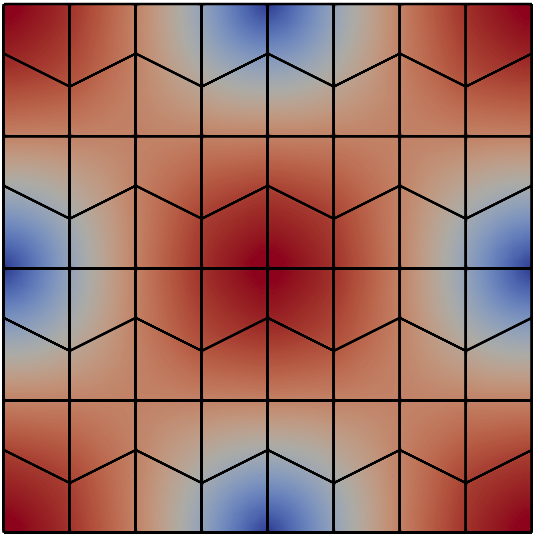
(a) Velocity magnitude

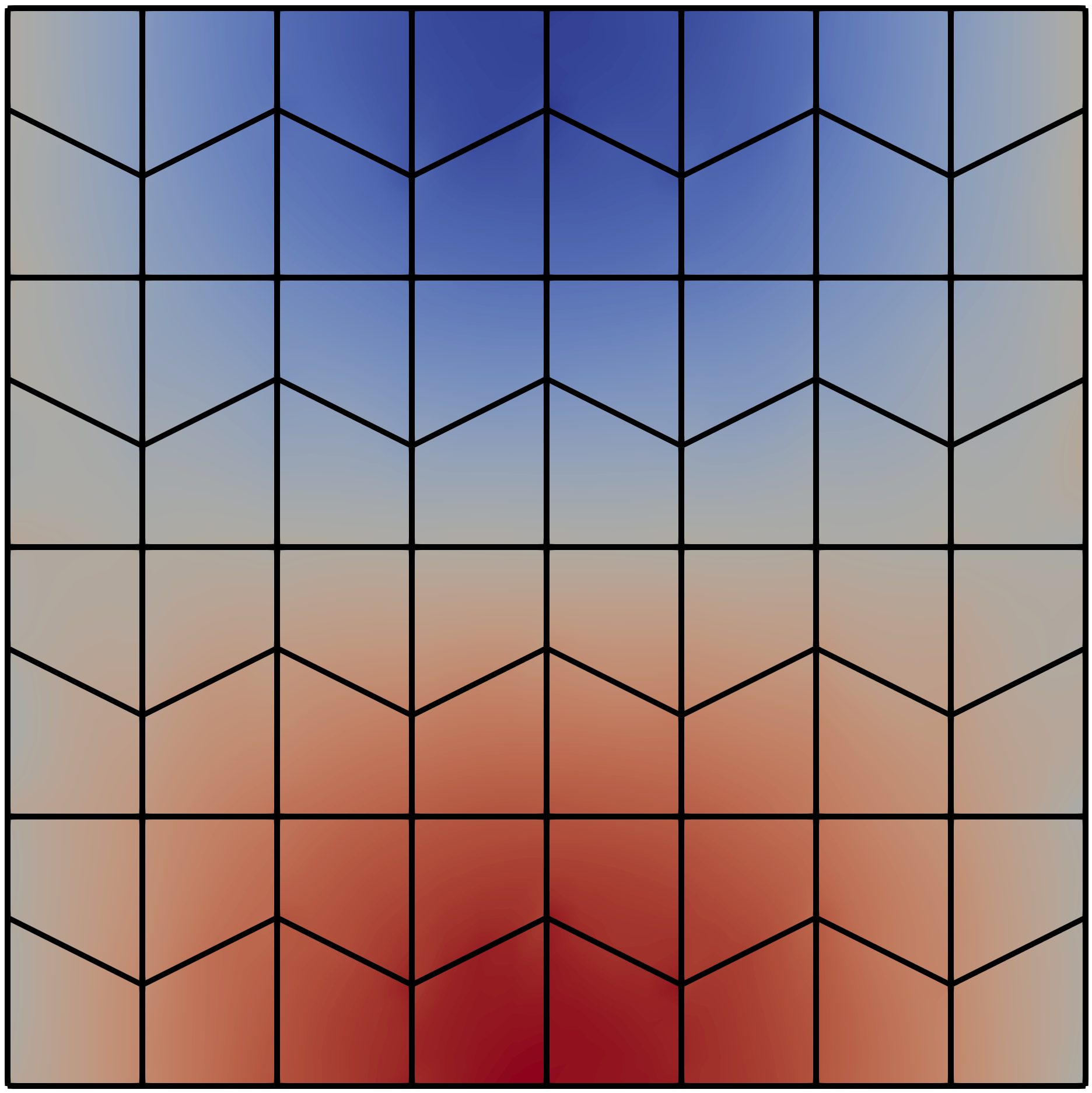
(b) Pressure

Figure 1: Computed solution to a simple Stokes problem on a mesh of trapezium shaped elements.

Figure 2 shows the $L^{2}(\Omega)$-norm of the error in the velocity field, $e_{u}$, and pressure field, $e_{p}$, as a function of $h$ for different values of $k$.

(a) Velocity field

(b) Pressure field

Figure 2: The $L^{2}(\Omega)$-norm of the error in the velocity and pressure fields as a function $h$. The velocity and pressure converge at rates $k+1$ and $k$, respectively.

The observed rate of convergence is $k+1$ for the velocity field and $k$ for the pressure field, which is in agreement with the theory presented in Section 4.

Figure 3 shows the $L^{2}(\Omega)$-norm of the error in the divergence of the velocity field, $e_{\nabla\cdot u}$, and the $L^{2}(\Gamma_{h})$-norm of the jump in the normal component of the velocity across element boundaries, $e_{\llbracket u\rrbracket}$, as a function of $h$. We compare the present method with a naive extension of the method from Rhebergen and Wells [24] to quadrilateral cells, which differs from the present method in that firstly, the finite element spaces are taken to be

$$V_{h}(\hat{K})\coloneqq[\mathbb{Q}_{k}(\hat{K})]^{d},\quad\bar{V}_{h}(\hat{F})\coloneqq[\mathbb{Q}_{k}(\hat{F})]^{d},\quad Q_{h}(\hat{K})\coloneqq\mathbb{Q}_{k-1}(\hat{K}),\quad\textnormal{and}\quad\bar{Q}_{h}(\hat{F})\coloneqq\mathbb{Q}_{k}(\hat{F});$$

and secondly, composition is used to map from the reference to the physical velocity space, rather than the contravariant Piola transform.

(a) Divergence error

(b) Jump error

Figure 3: The divergence and jump errors as a function of $h$ for the present method (PM) and the method from [24] (RW). Only the present method conserves mass exactly.

The computed velocity field for the present method is divergence-free to machine precision, which is in agreement with the theory presented in Section 3. By contrast, whilst the method from [24] gives a velocity field with continuous normal component across element boundaries to machine precision, the approximate velocity field is not exactly divergence-free.

Figure 4 shows $e_{u}$ and $e_{p}$ as a function of $h$ for the present method and the scheme presented in [24] with $k=2$ and $\nu\in\mathinner{\left\{1,10^{-3},10^{-6}\right\}}$.

(a) Velocity field

(b) Pressure field

Figure 4: Velocity ($e_{u}$) and pressure ($e_{p}$) errors as a function of $h$ with $k=2$ for the present method (PM) and the method presented in [24] (RW). The error in the velocity field is independent of the viscosity for the present method, in contrast to the method from [24].

For the present method, the error in the velocity does not depend on the viscosity, which is in agreement with the pressure robust estimate given in Theorem 1. By contrast, for the method from [24], the error in the velocity increases by several orders of magnitude as the viscosity is varied. This is because the computed velocity field is not exactly divergence-free, and thus the velocity error estimate contains the norm of the error in the pressure field scaled by the reciprocal of the viscosity [26]. In the case of the pressure field, for the present method, the error reduces as the viscosity decreases from $1$ to $10^{-3}$, but remains constant when the viscosity is further decreased to $10^{-6}$. This is consistent with the pressure error estimate given in Theorem 1, which contains the $H^{k}(\Omega)$-norm of the exact pressure field and the $H^{k+1}(\Omega)$ norm of the exact velocity field scaled by the viscosity. For large enough values of $\nu$, the velocity term dominates and therefore decreasing the viscosity reduces the error. However, when $\nu$ is small enough, the pressure term dominates, so reducing $\nu$ further has little effect. In fact, for small viscosities, the pressure converges at a rate $k+1$ instead of $k$. This is due to two factors: firstly, since the pressure term dominates, the rate of convergence is not limited by the $\mathcal{O}\mathinner{(h^{k})}$ velocity term. Secondly, for this problem, the exact pressure field is sufficiently regular to be in $H^{k+1}(\Omega)$, and since the pressure space contains all polynomials of degree at most $k$, the approximate pressure field converges at the rate $k+1$ (see [64] and [42, Remark 6.23] for more information). For the method from [24], varying the viscosity has little effect on the error in the pressure field.

6.2 A hydrostatic problem

We consider the hydrostatic problem from [2]. Let a fluid of unit viscosity occupy a unit square container with no slip between the fluid and the fixed container walls. The fluid is subjected to the force

$$f(x)=\begin{pmatrix}0\\ c(3x_{2}^{2}-x_{2}+1)\end{pmatrix},$$ (76)

where $c\in\mathbb{R}^{+}$ is a parameter. The exact solution is given by

$$u(x)=0\textnormal{ and }p(x)=c\left(x_{2}^{3}-\frac{x_{2}^{2}}{2}+x_{2}-\frac{7}{12}\right).$$ (77)

Note that the applied force is exactly balanced by the pressure gradient; the fluid is in hydrostatic equilibrium and changing the parameter $c$ only changes the pressure field.

The solution is computed using the present method and a Taylor–Hood scheme with $k=2$, $c=10^{4}$, and $\nu=1$ on a trapezium partition of $\Omega\coloneqq(0,1)^{2}$. Homogeneous Dirichlet boundary conditions are applied on $\partial\Omega$ for the velocity field. Figure 5 shows the magnitude of the approximate velocity field computed using each method, and the errors are tabulated in Table 1.

(a) Present method

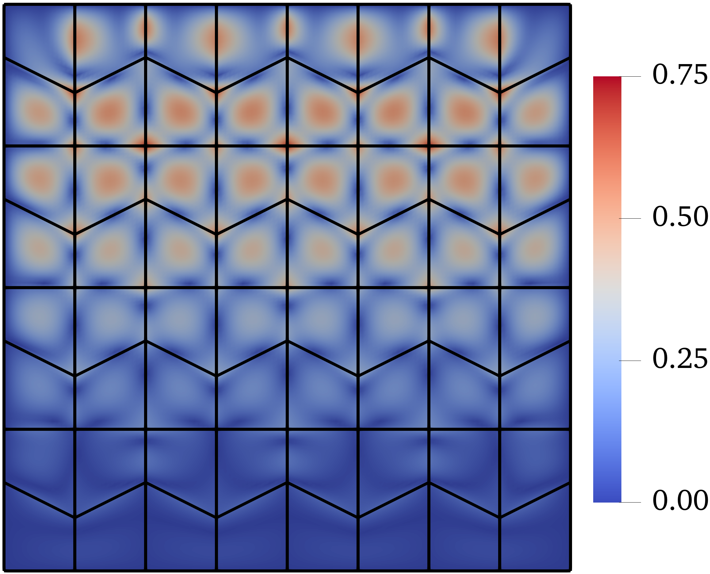
(b) Taylor–Hood

Figure 5: Magnitude of the computed velocity field for the hydrostatic problem with $k=2$ and $c=10^{4}$ for the present method and a Taylor–Hood scheme.

Table 1: Computed errors for the hydrostatic problem using the present method and a Taylor-Hood scheme.

Method	$e_{u}$	$e_{p}$	$e_{\nabla\cdot u}$	$e_{\llbracket u\rrbracket}$
Present	$1.10\text{\times}{10}^{-13}$	$0.447$	$6.54\text{\times}{10}^{-13}$	$4.56\text{\times}{10}^{-14}$
Taylor-Hood	$0.226$	$19.3$	$8.37$	$1.57\text{\times}{10}^{-16}$

The velocity field computed by the present method is exact to machine precision. By contrast, spurious flow can be seen in the velocity field computed by the Taylor–Hood scheme, which unlike the present method, does not preserve the invariance property of the Stokes equations.

6.3 A cylindrical bearing problem

We now present an example involving a curved boundary, which we approximate with curved elements. Whilst we showed in Section 3 that discretely divergence-free functions are exactly divergence-free for the curved elements we use in this example, our theoretical analysis used to obtain the pressure robust error estimate in Section 4 does not account for the fact that $\Omega_{h}$ does not coincide exactly with $\Omega$, and we have not proved Assumptions 2 to 8 for these elements. Despite this, it will be seen experimentally that the invariance property is preserved.

Consider a two-dimensional domain $\Omega\coloneqq\left\{x_{1}^{2}+x_{2}^{2}<r_{\rm{o}}^{2}\right\}\setminus\left\{x_{1}^{2}+(x_{2}+e)^{2}<r_{\rm{i}}^{2}\right\}$ bounded by inner and outer circles of radii $r_{\rm{i}}$ and $r_{\rm{o}}$ respectively. Let $e$ denote the offset between their centres in the $x_{2}$-direction. On the inner and outer boundaries, the tangential component of the velocity is prescribed as $u_{\rm{i}}$ and $u_{\rm{o}}$ respectively, and the normal component is set to zero. The applied force is taken to be zero. This type of flow has an analytical solution which can be found in [65].

We take $r_{\rm{i}}=0.7$, $r_{\rm{o}}=1$, $e=0.15$, $u_{\rm{i}}=1$, and $u_{\rm{o}}=0$, and use an unstructured mesh containing both quadrilateral and triangular cells. Polynomial geometric mappings of degree four are used to curve the cells on the boundary to ensure it is represented with sufficient accuracy. The computed solution for $k=3$ is presented in Fig. 6.

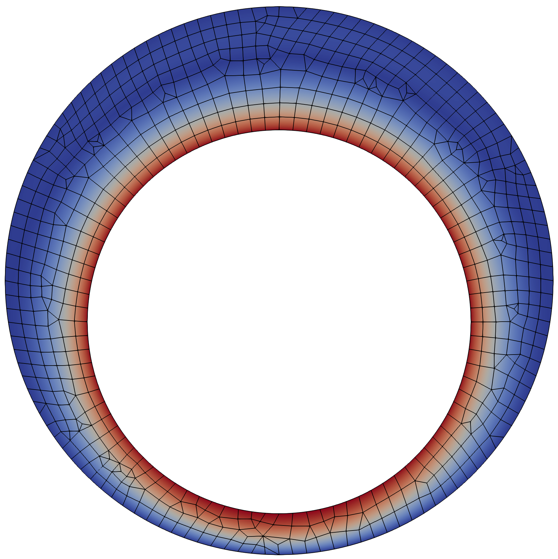
(a) Velocity field magnitude

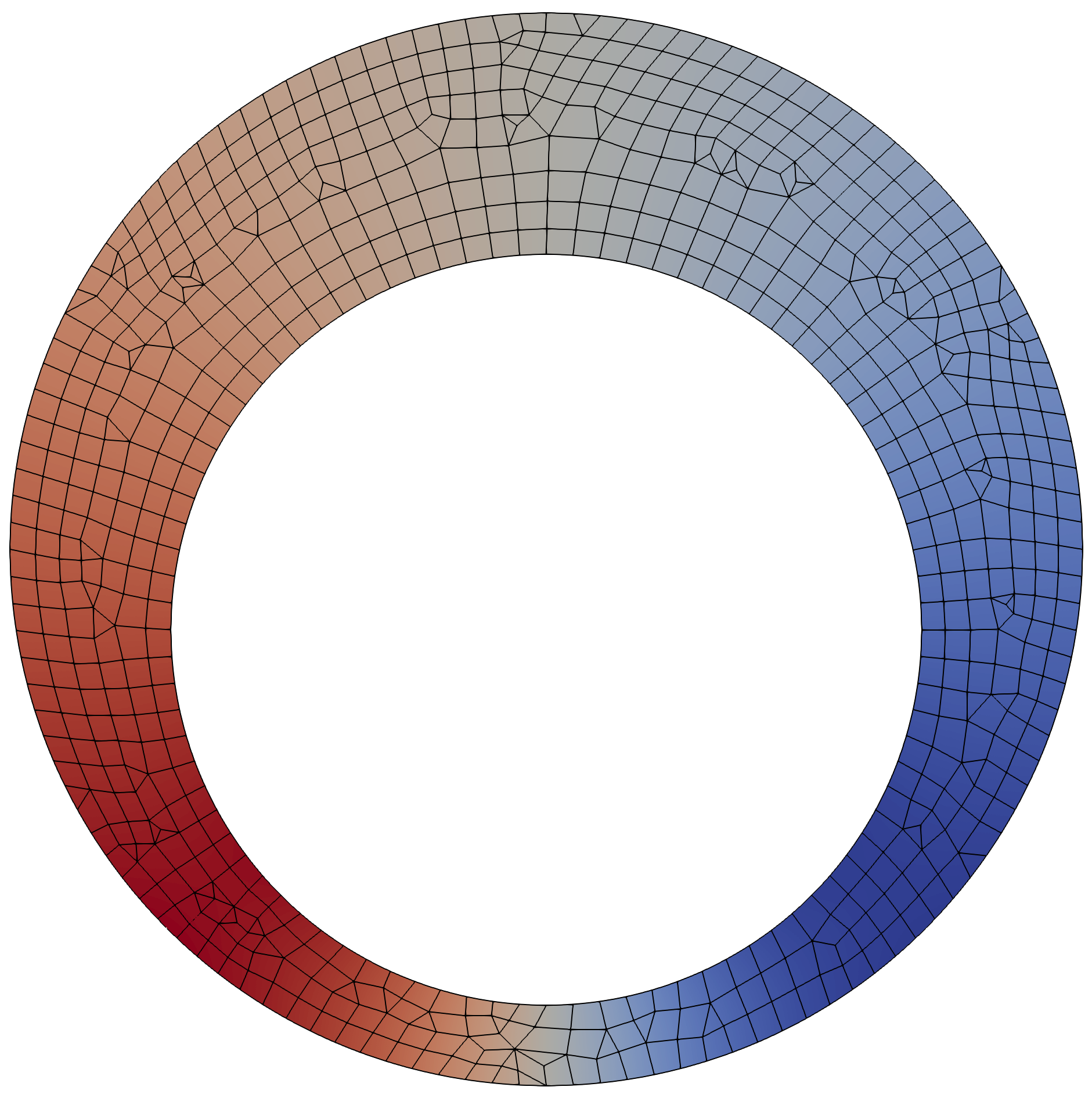
(b) Pressure field

Figure 6: The computed velocity magnitude and pressure fields for the cylindrical bearing problem with $k=3$.

Figure 7 shows that the computed velocity converges at the rate $k+1$.

Figure 7: The $L^{2}(\Omega)$-norm of the error in the velocity field as a function of $h$. The convergence rate of the velocity is $k+1$.

If curved cells had not been used on the boundary, values of $k$ larger than $1$ would not have increased the rate of convergence of the velocity field due to the poor geometric approximation. Figure 8 shows $e_{\nabla\cdot u}$ and $e_{\llbracket u\rrbracket}$ for the present method and method from [24] as a function of $h$.

(a) Divergence error

(b) Jump error

Figure 8: The divergence and jump errors as a function of $h$ for the present method (PM) and the method from [24] (RW). The present method conserves mass exactly, the method from [24] does not.

Once again, the present method gives a velocity field that is exactly divergence-free to machine precision despite the presence of curved elements, which is in agreement with the theory presented in Section 3. By contrast, the method from [24] produces a velocity field that is $H(\rm{div};\Omega)$-conforming to machine precision but not exactly divergence-free.

Finally, we demonstrate that, despite the presence of curved elements in this test case, the present method preserves the invariance property of the Stokes equations at the discrete level. Let the source function be modified to

$$f(x)=c\nabla\left(\sin(\pi x_{2})\right),$$ (78)

where $c\in\mathbb{R}^{+}$ is a parameter. Since $f$ is a gradient field, it is irrotational and therefore is exactly balanced by the pressure gradient in the continuous problem, leaving the velocity field unchanged [2]. The solution was computed for the present method and the method from [24] with $k=2$ and $c$ ranging from $1$ to $10^{6}$. The results are presented in Fig. 9.

Figure 9: The error in the velocity field as a function of $h$ for the present method (PM) and the method from [24] (RW). The error in the velocity is independent of $c$ for the present method, in contrast to the method from [24].

For the present method, the velocity field is unchanged as $c$ is varied, which is in accordance with the physically correct behaviour. By contrast, the method from [24] does not enjoy this property.

7 Conclusions

We have developed and analysed a hybridized discontinuous Galerkin method for the Stokes problem on non-affine cells that maintains an exactly divergence-free velocity field. Elements are mapped using the contravariant Piola transform, ensuring that key properties hold on both the reference and physical (mapped) element. Optimal, pressure robust error estimates for the velocity field are proved for flat-faced quadrilateral cells. Our theoretical analysis is consistent with our numerical experiments, which demonstrate that invariance properties are preserved and the analytical error estimates achieved. The method developed in this paper opens up the application of high-order, pressure robust methods for problems with complex geometries, with future possibilities being analysis of high aspect ratio tensor-product cell meshes for boundary layers and the generalisation of the analysis results to other non-affine cell types.

Acknowledgements

Support from the Engineering and Physical Sciences Research Council for JPD (EP/L015943/1) and GNW (EP/W026635/1, EP/W00755X/1, EP/S005072/1) is gratefully acknowledged. SR gratefully acknowledges support from the Natural Sciences and Engineering Research Council of Canada through the Discovery Grant program (RGPIN-2023-03237). We further thank Aaron Baier-Reinio for discussions on the proof of Lemma 12 resulting in an improved inf-sup constant.

References

- Linke [2014] Alexander Linke. On the role of the Helmholtz decomposition in mixed methods for incompressible flows and a new variational crime. Computer Methods in Applied Mechanics and Engineering, 268:782–800, 2014. URL https://doi.org/10.1016/j.cma.2013.10.011.
- John et al. [2017] Volker John, Alexander Linke, Christian Merdon, Michael Neilan, and Leo G. Rebholz. On the divergence constraint in mixed finite element methods for incompressible flows. SIAM Review, 59(3):492–544, 2017. URL https://doi.org/10.1137/15m1047696.
- Hood and Taylor [1974] P. Hood and C. Taylor. Navier–Stokes equations using mixed interpolation. University of Alabama in Huntsville Press, 1974.
- Arnold et al. [1984] D. N. Arnold, F. Brezzi, and M. Fortin. A stable finite element method for the Stokes equations. CALCOLO, 21:337–344, 1984.
- Crouzeix and Raviart [1973] M. Crouzeix and P.-A. Raviart. Conforming and nonconforming finite element methods for solving the stationary Stokes equations I. Revue française d’automatique informatique recherche opérationnelle. Mathématique, 7(R3):33–75, 1973. URL https://doi.org/10.1051/m2an/197307R300331.
- Linke [2009] Alexander Linke. Collision in a cross-shaped domain – A steady 2d Navier–Stokes example demonstrating the importance of mass conservation in CFD. Computer Methods in Applied Mechanics and Engineering, 198(41-44):3278–3286, 2009. URL https://doi.org/10.1016/j.cma.2009.06.016.
- Evans [2011] John Andrew Evans. Divergence-free B-spline discretizations for viscous incompressible flows. The University of Texas at Austin, 2011. URL http://repositories.lib.utexas.edu/handle/2152/ETD-UT-2011-12-4506.
- Peters and Evans [2019] Eric L. Peters and John A. Evans. A divergence-conforming hybridized discontinuous Galerkin method for the incompressible Reynolds-averaged Navier–Stokes equations. International Journal for Numerical Methods in Fluids, 91(3):112–133, 2019. URL https://doi.org/10.1002/fld.4745.
- Maljaars [2019] Jakob Maljaars. When Euler meets Lagrange Particle-Mesh Modeling of Advection Dominated Flows. PhD thesis, TU Delft University, 2019. URL https://doi.org/10.4233/uuid:a400512d-966d-402a-a40a-fedf60acf22c.
- Arnold et al. [2006] Douglas N. Arnold, Richard S. Falk, and Ragnar Winther. Finite element exterior calculus, homological techniques, and applications. Acta Numerica, 15(2006):1–155, 2006. URL https://doi.org/10.1017/S0962492906210018.
- Scott and Vogelius [1985a] L. R. Scott and M. Vogelius. Norm estimates for a maximal right inverse of the divergence operator in spaces of piecewise polynomials. ESAIM: Mathematical Modelling and Numerical Analysis, 19(1):111–143, 1985a. URL https://doi.org/10.1051/m2an/1985190101111.
- Scott and Vogelius [1985b] L. R. Scott and M. Vogelius. Conforming finite element methods for incompressible and nearly incompressible continua. Large-Scale Computations in Fluid Mechanics, 1985b.
- Guzmán and Neilan [2014a] J. Guzmán and M. Neilan. Conforming and divergence-free Stokes elements on general triangular meshes. Math. Comp., 83:15–36, 2014a. URL http://doi.org/10.1090/S0025-5718-2013-02753-6.
- Guzmán and Neilan [2014b] J. Guzmán and M. Neilan. Conforming and divergence-free Stokes elements in three dimensions. IMA J. Numer. Anal., 34:1489–1508, 2014b. URL http://doi.org/10.1093/imanum/drt053.
- Neilan and Sap [2018] Michael Neilan and Duygu Sap. Macro Stokes elements on quadrilaterals. International Journal of Numerical Analysis and Modeling, 15(4-5):729–745, 2018.
- Qin [1994] Jinshui Qin. On the convergence of some low order mixed finite elements for incompressible fluids. PhD thesis, Pennsylvania State University, 1994.
- Cockburn et al. [2004] Bernardo Cockburn, Guido Kanschat, and Dominik Schötzau. A locally conservative LDG method for the incompressible Navier–Stokes equations. Mathematics of Computation, 74(251):1067–1096, 2004. URL https://doi.org/10.1090/S0025-5718-04-01718-1.
- Cockburn et al. [2007] Bernardo Cockburn, Guido Kanschat, and Dominik Schötzau. A note on discontinuous Galerkin divergence-free solutions of the Navier–Stokes equations. Journal of Scientific Computing, 31(1-2):61–73, 2007. URL https://doi.org/10.1007/s10915-006-9107-7.
- Wang and Ye [2007] Junping Wang and Xiu Ye. New finite element methods in computational fluid dynamics by (div) elements. SIAM Journal on Numerical Analysis, 45(3):1269–1286, 2007. URL https://doi.org/10.1137/060649227.
- Boffi et al. [2013] Daniele Boffi, Franco Brezzi, and Michel Fortin. Mixed Finite Element Methods and Applications, volume 44 of Springer Series in Computational Mathematics. Springer Berlin Heidelberg, 2013. ISBN 978-3-642-36518-8. URL https://doi.org/10.1007/978-3-642-36519-5.
- Cockburn et al. [2009] Bernardo Cockburn, Jayadeep Gopalakrishnan, and Raytcho Lazarov. Unified hybridization of discontinuous Galerkin, mixed, and continuous Galerkin methods for second order elliptic problems. SIAM Journal on Numerical Analysis, 47(2):1319–1365, 2009. URL https://doi.org/10.1137/070706616.
- Cockburn and Gopalakrishnan [2009] Bernardo Cockburn and Jayadeep Gopalakrishnan. The derivation of hybridizable discontinuous Galerkin methods for Stokes flow. SIAM Journal on Numerical Analysis, 47(2):1092–1125, 2009. URL https://doi.org/10.1137/080726653.
- Lehrenfeld and Schöberl [2016] Christoph Lehrenfeld and Joachim Schöberl. High order exactly divergence-free hybrid discontinuous Galerkin methods for unsteady incompressible flows. Computer Methods in Applied Mechanics and Engineering, 307:339–361, 2016. URL https://doi.org/10.1016/j.cma.2016.04.025.
- Rhebergen and Wells [2018a] Sander Rhebergen and Garth N. Wells. A hybridizable discontinuous Galerkin method for the Navier–Stokes equations with pointwise divergence-free velocity field. Journal of Scientific Computing, 76(3):1484–1501, 2018a. URL https://doi.org/10.1007/s10915-018-0671-4.
- Rhebergen and Wells [2017] Sander Rhebergen and Garth N. Wells. Analysis of a hybridized/interface stabilized finite element method for the Stokes equations. SIAM Journal on Numerical Analysis, 55(4):1982–2003, 2017. URL https://doi.org/10.1137/16M1083839.
- Rhebergen and Wells [2020] Sander Rhebergen and Garth N. Wells. An embedded–hybridized discontinuous Galerkin finite element method for the Stokes equations. Computer Methods in Applied Mechanics and Engineering, 358(112619), 2020. URL https://doi.org/10.1016/j.cma.2019.112619.
- Labeur and Wells [2012] Robert Jan Labeur and Garth N. Wells. Energy stable and momentum conserving hybrid finite element method for the incompressible Navier–Stokes equations. SIAM Journal on Scientific Computing, 34(2):A889–A913, 2012. URL https://doi.org/10.1137/100818583.
- Carrero et al. [2005] Jesús Carrero, Bernardo Cockburn, and Dominik Schötzau. Hybridized globally divergence-free LDG methods. Part I: The Stokes problem. Mathematics of Computation, 75(254):533–563, 2005. URL https://doi.org/10.1090/s0025-5718-05-01804-1.
- Cockburn and Gopalakrishnan [2005a] Bernardo Cockburn and Jayadeep Gopalakrishnan. Incompressible finite elements via hybridization. Part I: The Stokes system in two space dimensions. SIAM Journal on Numerical Analysis, 43(4):1627–1650, 2005a. URL https://doi.org/10.1137/04061060X.
- Cockburn and Gopalakrishnan [2005b] Bernardo Cockburn and Jayadeep Gopalakrishnan. Incompressible finite elements via hybridization. Part II: The Stokes system in three space dimensions. SIAM Journal on Numerical Analysis, 43(4):1651–1672, 2005b. URL https://doi.org/10.1137/040610659.
- Neilan and Otus [2021] Michael Neilan and Baris Otus. Divergence-free Scott–Vogelius elements on curved domains. SIAM Journal on Numerical Analysis, 59(2):1090–1116, 2021. URL https://doi.org/10.1137/20M1360098.
- Schroeder and Lube [2018] Philipp W. Schroeder and Gert Lube. Divergence-free (div)-FEM for time-dependent incompressible flows with applications to high Reynolds number vortex dynamics. Journal of Scientific Computing, 75(2):830–858, 2018.
- Ern and Guermond [2004] Alexandre Ern and Jean-Luc Guermond. Theory and Practice of Finite Elements. Applied Mathematical Sciences. Springer, New York, NY, 2004. ISBN 978-1-4419-1918-2. URL https://doi.org/10.1007/978-1-4757-4355-5.
- Bossavit [1998] Alain Bossavit. Computational Electromagnetism. Variational Formulations, Complementarity, Edge Elements. Elsevier, 1998. URL https://doi.org/10.1016/B978-0-12-118710-1.X5000-4.
- Rognes et al. [2010] Marie E. Rognes, Robert C. Kirby, and Anders Logg. Efficient assembly of (div) and (curl) conforming finite elements. SIAM Journal on Scientific Computing, 31(6):4130–4151, 2010. URL https://doi.org/10.1137/08073901X.
- Arnold et al. [2005] Douglas N. Arnold, Daniele Boffi, and Richard S. Falk. Quadrilateral (div) finite elements. SIAM Journal on Numerical Analysis, 42(6):2429–2451, 2005. URL https://doi.org/10.1137/S0036142903431924.
- Raviart and Thomas [1977] P. A. Raviart and J. M. Thomas. A mixed finite element method for 2-nd order elliptic problems. In Ilio Galligani and Enrico Magenes, editors, Mathematical Aspects of Finite Element Methods, pages 292–315, Berlin, Heidelberg, 1977. Springer Berlin Heidelberg. ISBN 978-3-540-37158-8.
- Brezzi et al. [1985] Franco Brezzi, Jim Douglas, and L. D. Marini. Two families of mixed finite elements for second order elliptic problems. Numerische Mathematik, 47(2):217–235, 1985. URL https://doi.org/10.1007/BF01389710.
- Falk et al. [2011] Richard S. Falk, Paolo Gatto, and Peter Monk. Hexahedral h(div) and h(curl) finite elements. ESAIM: Mathematical Modelling and Numerical Analysis, 45(1):115–143, 2011. doi: 10.1051/m2an/2010034.
- Ern and Guermond [2021] Alexandre Ern and Jean-Luc Guermond. Finite Elements I, volume 72 of Texts in Applied Mathematics. Springer International Publishing, 2021. URL https://doi.org/10.1007/978-3-030-56341-7.
- Georgoulis [2003] E. H. Georgoulis. Discontinuous Galerkin methods on shape-regular and anisotropic meshes. Doctor of Philosophy Thesis, 2003.
- Di Pietro and Ern [2012] Daniele Antonio Di Pietro and Alexandre Ern. Mathematical Aspects of Discontinuous Galerkin Methods, volume 69 of Mathématiques et Applications. Springer Berlin Heidelberg, Berlin, Heidelberg, 2012. URL https://doi.org/10.1007/978-3-642-22980-0.
- Wheeler et al. [2012] Mary Wheeler, Guangri Xue, and Ivan Yotov. A multipoint flux mixed finite element method on distorted quadrilaterals and hexahedra. Numerische Mathematik, 121(1):165–204, 2012. URL https://doi.org/10.1007/s00211-011-0427-7.
- Ingram et al. [2010] Ross Ingram, Mary F. Wheeler, and Ivan Yotov. A multipoint flux mixed finite element method on hexahedra. SIAM Journal on Numerical Analysis, 48(4):1281–1312, 2010. URL https://doi.org/10.1137/090766176.
- Evans and Hughes [2013] John A. Evans and Thomas J. R. Hughes. Explicit trace inequalities for isogeometric analysis and parametric hexahedral finite elements. Numerische Mathematik, 123(2):259–290, 2013. URL https://doi.org/10.1007/s00211-012-0484-6.
- Brezzi and Fortin [1991] Franco Brezzi and Michel Fortin. Mixed and Hybrid Finite Element Methods, volume 15 of Springer Series in Computational Mathematics. Springer, New York, 1991. URL https://doi.org/10.1007/978-1-4612-3172-1.
- Du and Sayas [2019] Shukai Du and Francisco-Javier Sayas. An Invitation to the Theory of the Hybridizable Discontinuous Galerkin Method. SpringerBriefs in Mathematics. Springer International Publishing, 2019. URL https://doi.org/10.1007/978-3-030-27230-2.
- Brenner and Scott [2008] Susanne C. Brenner and L. Ridgway Scott. The Mathematical Theory of Finite Element Methods, volume 15 of Texts in Applied Mathematics. Springer New York, New York, NY, 2008. URL https://doi.org/10.1007/978-0-387-75934-0.
- Bernardi and Girault [1998] Christine Bernardi and Vivette Girault. A local regularization operator for triangular and quadrilateral finite elements. SIAM Journal on Numerical Analysis, 35(5):1893–1916, 1998. URL https://doi.org/10.1137/S0036142995293766.
- Rhebergen and Wells [2018b] Sander Rhebergen and Garth N. Wells. Preconditioning of a hybridized discontinuous Galerkin finite element method for the Stokes equations. Journal of Scientific Computing, 77(3):1936–1952, 2018b. URL https://doi.org/10.1007/s10915-018-0760-4.
- Howell and Walkington [2011] Jason S. Howell and Noel J. Walkington. Inf-sup conditions for twofold saddle point problems. Numerische Mathematik, 118(4):663–693, 2011. URL https://doi.org/10.1007/s00211-011-0372-5.
- Scroggs et al. [2022a] Matthew W. Scroggs, Jørgen S. Dokken, Chris N. Richardson, and Garth N. Wells. Construction of arbitrary order finite element degree-of-freedom maps on polygonal and polyhedral cell meshes. ACM Trans. Math. Softw., 48(2), 2022a. URL https://doi.org/10.1145/3524456.
- Scroggs et al. [2022b] Matthew W. Scroggs, Igor A. Baratta, Chris N. Richardson, and Garth N. Wells. Basix: a runtime finite element basis evaluation library. Journal of Open Source Software, 7(73):3982, 2022b. URL https://doi.org/10.21105/joss.03982.
- Logg et al. [2012] A. Logg, K.-A. Mardal, and G. N. Wells, editors. Automated Solution of Differential Equations by the Finite Element Method, volume 84 of Lecture Notes in Computational Science and Engineering. Springer, 2012. URL http://dx.doi.org/10.1007/978-3-642-23099-8.
- dol [2023] DOLFINx. https://github.com/FEniCS/dolfinx, 2023. Accessed: 2023-06-02.
- Schöberl [2014] Joachim Schöberl. C++ 11 implementation of finite elements in NGSolve. Technical Report ASC-2014-30, Institute for Analysis and Scientific Computing, 2014. URL https://www.asc.tuwien.ac.at/~schoeberl/wiki/publications/ngs-cpp11.pdf.
- Amestoy et al. [2001] P.R. Amestoy, I. S. Duff, J. Koster, and J.-Y. L’Excellent. A fully asynchronous multifrontal solver using distributed dynamic scheduling. SIAM Journal on Matrix Analysis and Applications, 23(1):15–41, 2001.
- Amestoy et al. [2019] P.R. Amestoy, A. Buttari, J.-Y. L’Excellent, and T. Mary. Performance and Scalability of the Block Low-Rank Multifrontal Factorization on Multicore Architectures. ACM Transactions on Mathematical Software, 45:2:1–2:26, 2019.
- Balay et al. [2023a] Satish Balay, Shrirang Abhyankar, Mark F. Adams, et al. PETSc Web page, 2023a. URL https://petsc.org/.
- Balay et al. [2023b] Satish Balay, Shrirang Abhyankar, Mark F. Adams, et al. PETSc/TAO users manual. Technical Report ANL-21/39 - Revision 3.19, Argonne National Laboratory, 2023b.
- Balay et al. [1997] Satish Balay, William D. Gropp, Lois Curfman McInnes, and Barry F. Smith. Efficient management of parallelism in object oriented numerical software libraries. In E. Arge, A. M. Bruaset, and H. P. Langtangen, editors, Modern Software Tools in Scientific Computing, pages 163–202. Birkhäuser Press, 1997.
- Davis [2004] Timothy A. Davis. Algorithm 832: Umfpack v4.3—an unsymmetric-pattern multifrontal method. ACM Trans. Math. Softw., 30(2):196–199, 2004. URL https://doi.org/10.1145/992200.992206.
- cod [2023] Supplimentary code for the numerical examples. https://github.com/jpdean/cmame_non_affine_hdg_paper_code, 2023. Accessed: 01-09-23.
- Arnold et al. [2002] Douglas N. Arnold, Daniele Boffi, and Richard S. Falk. Approximation by quadrilateral finite elements. Mathematics of Computation, 71(239):909–922, 2002. URL https://doi.org/10.1090/s0025-5718-02-01439-4.
- Wannier [1950] Gregory H. Wannier. A contribution to the hydrodynamics of lubrication. Quarterly of Applied Mathematics, 8(1):1–32, 1950. URL https://doi.org/10.1090/qam/37146.