COURIER: Contrastive User Intention Reconstruction
for Large-Scale Pre-Train of Image Features

Abstract.

With the development of the multi-media internet, visual characteristics have become an important factor affecting user interests. Thus, incorporating visual features is a promising direction for further performance improvements in click-through rate (CTR) prediction. However, we found that simply injecting the image embeddings trained with established pre-training methods only has marginal improvements. We attribute the failure to two reasons: First, The pre-training methods are designed for well-defined computer vision tasks concentrating on semantic features, and they cannot learn personalized interest in recommendations. Secondly, pre-trained image embeddings only containing semantic information have little information gain, considering we already have semantic features such as categories and item titles as inputs in the CTR prediction task. We argue that a pre-training method tailored for recommendation is necessary for further improvements. To this end, we propose a recommendation-aware image pre-training method that can learn visual features from user click histories. Specifically, we propose a user interest reconstruction module to mine visual features related to user interests from behavior histories. We further propose a contrastive training method to avoid collapsing of embedding vectors. We conduct extensive experiments to verify that our method can learn users’ visual interests, and our method achieves $0.46\%$ improvement in offline AUC and $0.88\%$ improvement in Taobao online GMV with p-value$<0.01$.

1. Introduction

Predicting the click-through rate (CTR) is an essential task in recommendation systems based on deep learning(Zhang et al., 2021; Zhou et al., 2019; Feng et al., 2019). Typically, CTR models measure the probability that a user will click on an item based on the user’s profile and behavior history(Zhou et al., 2019; Feng et al., 2019), such as clicking, purchasing, adding cart, etc. The behavior histories are represented by sequences of item IDs, titles, and some statistical features, such as monthly sales and favorable rate.

Intuitively, the visual images of the items are also important in online item recommendation, especially in categories such as women’s clothing. However, our experiments indicate that utilizing embeddings pre-trained with existing image pre-training methods(Chen et al., 2020a; Chen and He, 2021; Radford et al., 2021) only have a marginal or even negative impact on the corresponding downstream CTR prediction task. We attribute this failure to two reasons: First, the pre-training tasks do not fit the CTR task. Existing pre-training methods are designed and tested for computer vision (CV) tasks, such as classification, segmentation, captioning, etc. The CV tasks have a precise definition of the target labels, such as the class of an image. While in the recommendation scenario, the user’s preference for visual appearance is usually vague and imprecise. For example, a user may think a cloth looks cute, while another may not. Thus, existing pre-training methods may not be able to learn such visual characteristics. Secondly, the information learned through the pre-training methods may be useless in our scenario. We may hope that the semantic information contained in the pre-trained embeddings (classes, language description, etc.) can improve the CTR prediction. However, such information can be directly used in item recommendations. For example, we have the categories, item titles, and style tags that are provided by the merchants, which are already used in our CTR model. Thus, a pre-trained model performs well at predicting categories or titles has little new information and won’t improve on the recommendation tasks.

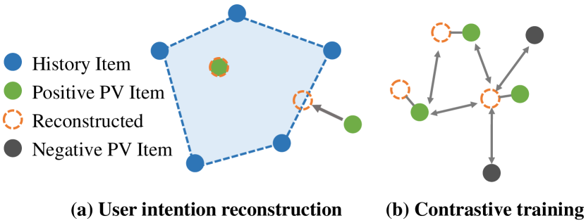
Figure 1. The contrastive user intention reconstruction (Courier) method. (a) The items in the user click history are used to reconstruct the embeddings of positive PV items. An embedding will be pushed to approach the corresponding reconstruction if the reconstruction is not perfect. (b) To avoid trivial degeneration of the embeddings, we propose a contrastive framework: While the embeddings and corresponding reconstructions are pushed closer, unmatched embeddings and reconstructions are pushed further apart.

We argue that to boost the performance of downstream CTR prediction tasks, the pre-training method should be aware of the downstream task and should also be decoupled from the CTR task to reduce computation. To achieve this goal, we propose a COntrastive UseR IntEntion Reconstruction (Courier) method. Our method is based on an intuitive assumption: An item clicked by a user is likely to have visual characteristics similar to some of the clicking history items. For example, a user that has clicked on a white dress and a red T-shirt may also be interested in a red dress. However, the visual characteristics that affect the users’ choices may not be as clear as in the example, such as looking cute or cool. To mine the visual features related to user interests, we propose reconstructing the next clicking item with a cross-attention mechanism on the clicking history items. The reconstruction can be interpreted by a weighted sum of history item embeddings, as depicted in Figure. 1 (a), which can be trained end-to-end. Minimizing the reconstruction loss alone will lead to a trivial solution: all the embeddings collapse to the same value. Thus, we propose to optimize a contrastive loss that not only encourages lower reconstruction error, but also push embeddings of un-clicked items further apart, as depicted in Figure. 1 (b). We conducted various experiments to verify our motivation and design of the method. In offline experiments, our method achieves $0.46\%$ absolute improvement on AUC and $10.4\%$ relative improvement on NDCG@10 compared to a strong baseline. In online A/B tests, we achieve $0.88\%$ improvement on GMV in the women’s clothing category, which is significant considering the volume of the Taobao search engine.

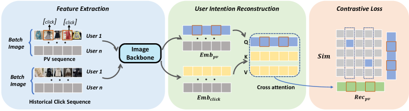
Figure 2. The contrastive user intention reconstruction method. The images are fed into the image backbone model to obtain the corresponding embeddings. The embeddings of PV sequences are blue-colored, and the embeddings of click sequences are yellow-colored. The reconstructions are in green. Red boxes denote positive PV items.

Our contribution can be summarized as follows:

• To pre-train image embeddings containing users’ visual preferences, we propose a user interest reconstruction method, which can mine latent user interests from history click sequences.

• The user interest reconstruction alone may lead to a collapsed solution. To solve this problem, we propose a contrastive training method that utilizes the negative PV items efficiently.

• We conduct extensive experiments to verify the effectiveness of our method. Our experimental results show that our method can learn meaningful visual concepts, and the model can generalize to unseen categories.

2. Related Work

From collaborative filtering(Schafer et al., 2007; Linden et al., 2003; Koren et al., 2009) to deep learning based recommender systems(Zhang et al., 2019; Huang et al., 2013; He et al., 2017; Hidasi et al., 2016), IDs and categories (user IDs, item IDs, advertisement IDs, tags, etc.) are the essential features in item recommendation systems, which can straightforwardly represent the identities. However, with the development of the multi-media internet, ID features alone can hardly cover all the important information. Thus, recommendations based on content such as images, videos, and texts have become an active research field in recommender systems. In this section, we briefly review the related work and discuss their differences compared with our method.

2.1. Content-based recommendation

In general, content is more important when the content itself is the concerned information. Thus, the content-based recommendation has already been applied in news(Wu et al., 2021b; Li et al., 2022; Bi et al., 2022; An et al., 2019; Xiao et al., 2022; Ding et al., 2021), music(van den Oord et al., 2013; Wang and Wang, 2014), image(Wu et al., 2020), and video(Covington et al., 2016; Lee and Abu-El-Haija, 2017; Wei et al., 2019; Lei et al., 2021) recommendations.

Research on the content-based recommendation in the item recommendation task is much fewer because of the dominating ID features. Early applications of image features typically use image embeddings extracted from a pre-trained image classification model, such as (He and McAuley, 2016, 2016; McAuley et al., 2015; Hou et al., 2019). The image features adopted by these methods are trained on general classification datasets such as ImageNet(Deng et al., 2009), which may not fit recommendation tasks. Thus, Dong et al. (2022) proposes to train on multi-modal data from recommendation task. However, Dong et al. (2022) does not utilize any recommendation labels such as clicks and payments, which will have marginal improvement if we are already using information from other modalities, as we analyze in Section. 3.3.

With the increase in computing power, some recent papers propose to train item recommendation models end-to-end with image feature networks(Anonymous, 2023; Elsayed et al., 2022; Wang et al., 2022b). However, the datasets used in these papers are much smaller than our application scenario. For example, Wang et al. (2022b) uses a dataset consisting of 25 million interactions. While in our online system, average daily interactions in a single category (women’s clothing) are about 850 million. We found it infeasible to train image networks in our scenario end-to-end, which motivates our decoupled two-stage framework with user-interest-aware pre-training.

2.2. Pre-training of image features

Self-supervised pre-training has been a hot topic in recent years. We classify the self-supervised learning methods into two categories: Augmentation-based and prediction-based.

Augmentation-based. Taking image pre-training as an example, the augmentation-based methods generate multiple different views of an image by random transformations, then the model is trained to pull the embeddings of different views closer and push other embeddings (augmented from different images) further. SimCLR(Chen et al., 2020a), SimSiam(Chen and He, 2021), BYOL(Grill et al., 2020) are some famous self-supervised methods in this category. These augmentation-based methods do not perform well in the item recommendation task as shown in our experiments in Section. 4.5. Since the augmentations are designed for classification (or segmentation, etc.) tasks, they change the visual appearance of the images without changing their semantic class, which contradicts the fact that visual appearance is also important in recommendations (e.g., color, shape, etc.).

Prediction-based. If the data can be split into more than one part, we can train a model taking some of the parts as inputs and predict the rest parts, which is the basic idea of prediction-based pre-training. Representative prediction-based methods include BERT(Devlin et al., 2019), CLIP(Radford et al., 2021), GPT(Brown et al., 2020), VL-BERT(Su et al., 2020), etc. The prediction-based methods can be used to train multi-modal recommendation data as proposed by Dong et al. (2022). However, if we are already utilizing multi-modal information, the improvements are limited, as shown in our experiments. To learn user interests information that can not be provided by other modalities, we argue that user behaviors should be utilized, as in our proposed method.

2.3. Contrastive learning in recommender systems

Contrastive learning methods are also adopted in recommendation systems in recent years. The most explored augmentation-based method is augmenting data by dropping, reordering, and masking some features(Yao et al., 2021; Liu et al., 2021a; Wang et al., 2022a; Liu et al., 2021c), items(Zhou et al., 2020; Xie et al., 2022; Qiu et al., 2022; Hou et al., 2022), and graph edges(Wu et al., 2021a). Prediction-based methods are also adopted for recommendation tasks, e.g., BERT4Rec(Sun et al., 2019) randomly masks some items and makes predictions. However, all these recommender contrastive learning methods concentrate on augmentation and pre-training with ID features, while our method tackles with pre-training of image features.

3. The proposed method

We briefly introduce some essential concepts and notations, then introduce our pre-training and downstream CTR model in detail.

3.1. Preliminary

Background. Modeling user preference (user portrait) is one of the most important problems in personalized recommender systems. Currently, the best-performing method utilizes the attention mechanism to model long-term user interests, where the user interests are mainly reflected by the history of clicking, purchasing, or shopping cart, which are lists of items. For example, a user that has clicked a red dress is more likely to click another red dress in the future, which reflects the user’s preference for red dresses. The general cases, however, are much more complicated: Even the users themselves may not be able to describe their preferences explicitly. For example, a user may prefer "lovely clothing." However, the exact visual appearance of "lovely clothing" is not well defined and may vary between users. Such preference information cannot be described by the available data exactly, such as category and style tags provided by the merchants. Typically, the features of items are their IDs, titles, tags, prices, and some statistical values, such as monthly sales and favorable rates. Among them, numerical features are directly concatenated; the categorical features are converted to their corresponding embeddings then concatenated with numerical features.

Notations. A data sample for CTR prediction in item search can be represented with a tuple of (user, item, query, label). A user searches for a query text, and several items are shown to the user. Then the items that the user clicked are labeled as positive and negative otherwise. When a user views a page, we have a list of items that are presented to the user, we call them page-view (PV) items. The length of this PV list is denoted by $l_{pv}$. Each PV item has a cover image, denoted by $Img_{pv}^{j}$, where $0\leq j<l_{pv}$. The corresponding click labels are denoted by $y_{pv}^{j}$, where $y_{pv}^{j}\in\{0,1\}$. Each user has a list of clicked item history, the image of each item is denoted by $Img_{click}^{k}$. $0\leq k<l_{click}$, where $l_{click}$ is the length of click history. The $l_{pv}$ and $l_{click}$ may vary by different users and pages, we trim or pad to the same length practically.

Attention. An attention layer is defined as follows:

(1) $$\operatorname{Attention}(Q,K,V)=\operatorname{softmax}(\frac{QK^{T}}{\sqrt{d_{K}}})V$$

where $Q$ is the query matrix, $K$ is the key matrix, $V$ is the value matrix. The mechanism of the attention layer can be interpreted intuitively: For each query, a similarity score is computed with every key, the values corresponding to keys are weighted by their similarity scores and summed up to obtain the outputs. We refer interested readers to Vaswani et al. (2017) for more details of the attention mechanism.

3.2. Contrastive User Intention Reconstruction

We make an essential assumption that the users’ preferences are fully described by their clicking history, and a newly clicked item be characterized by all the past clicked items. Intuitively, our assumption can be described as follows: Every item has some specific characteristics, such as lovely, sweet, gorgeous, etc. Assuming a user has clicked on three items with characteristics (A, B), (A, C), (B, D), respectively. When a user clicks a new item, we don’t know what the characteristics of the new item are, but we assume the new item can be reconstructed by some of the characteristics of the previously clicked items. That is, we assume that the characteristics of the new item may be (A, D), (A, B, C), but not (A, E). Such an assumption may not hold precisely, since the new item may indeed contain some new characteristics that does not exist in the click history. In such case, we want the model to recover as many common characteristics as possible. To this end, we propose a user-interest reconstruction method to learn to extract such characteristics that are related to user interests.

3.2.1. User intention reconstruction

In the following discussion, we only consider a single line of data (a PV list and corresponding list of user click history), the batch training method will be discussed later. We use $Img_{pv}$ and $Img_{click}$ to denote the matrix of all the $l_{pv}$ and $l_{click}$ images. All the images are fed to the image backbone (IB) to get their embeddings. We denote the embeddings as $Emb_{pv}^{j}=IB(Img_{pv}^{j})$ and $Emb_{click}^{k}=IB(Img_{click}^{k})$ correspondingly. In our user interest reconstruction method, we treat the embeddings of PV images $Emb_{pv}$ as queries $Q$, and we input the embeddings of click images $Emb_{click}$ as values $V$ and keys $K$. Then the user interest reconstruction layer can be calculated by

(2) $$Rec_{pv}^{j} =\operatorname{Attention}(Emb_{pv}^{j},Emb_{click},Emb_{click})$$

(3) $$=\sum\alpha_{k}Emb_{click}^{k}$$

where $\alpha\sim softmax\left(Emb_{pv}^{j}Emb_{click}^{T}\right)$. $\alpha_{k}$ is the attention on $k$th history click item. The reason for its name is that the attention layer forces the outputs to be a weighted sum of the embeddings of click sequences. Thus, the output space is limited to the combination of $Emb_{click}$ within a simplex as depicted in Figure. 1 (a).

3.2.2. Contrastive training method

Algorithm 1 Courier Pseudocode, PyTorch-like

⬇

1# backbone, attention: image backbone and attention models.

2# size: dimension of embeddings.

3# pv_n, click_n: number of page-view and click history items.

4

5for img_pv, img_click, labels in dataloader:

6 # Calculate the embeddings.

7 emb_p, emb_c = backbone(img_pv), backbone(img_click)

8 # emb_p.shape = (batch_size, pv_n, size)

9 # emb_c.shape = (batch_size, pv_n, click_n, size)

10 # labels.shape = (batch_size, pv_n)

11

12 # Flatten batch data and calculate reconstructions.

13 emb_p = reshape(emb_p, (batch_size*pv_n, size))

14 emb_c = reshape(emb_c, (batch_size*pv_n, click_n, size))

15 rec_pv = attention(emb_p, emb_c, emb_c)

16 # rec_pv.shape = (batch_size*pv_n, size)

17

18 # Calculate similarity matrix Sim(j0, j1)

19 emb_p = normalize(emb_p, dim=1) # normalize

20 rec_pv = normalize(rec_pv, dim=1) # normalize

21 sim_matrix = emb_p @ rec_pv.t()

22

23 # Calculate the contrastive loss

24 labels = reshape(labels, (batch_size*pv_n))

25 log_prob = log_softmax(sim_matrix / tau, dim=0)

26 loss = sum(-log_prob * diag(labels)) / (batch_size * pv_n)

27

28 loss.backward() # Calculate gradients by backpropagation

29 update(backbone, attention) # Update models by SGD

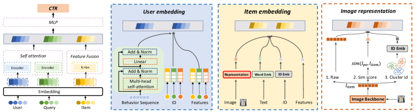
Figure 3. The downstream CTR model and image representation.

The user intention reconstruction module cannot prevent the trivial solution that all the embeddings collapse to the same value. Thus, we propose a contrastive method to train the user-interest reconstruction module.

With the PV embeddings $Emb_{pv}$, and the corresponding reconstructions $Rec_{pv}$. We calculate pairwise similarity score of $Emb_{pv}^{j_{0}}$ and $Rec_{pv}^{j_{1}}$:

(4) $$Sim(j_{0},j_{1})=\frac{{Emb_{pv}^{j_{0}}}^{T}Rec_{pv}^{j_{1}}}{||Emb_{pv}^{j_{0}}||\;||Rec_{pv}^{j_{1}}||}$$

Then we calculate the contrastive loss by

(5) $$L_{pv} =\mathcal{L}_{contrast}(Emb_{pv},Emb_{click},y)$$

(6) $$=\sum_{j_{0},j_{1}}-\log\left(\frac{e^{Sim(j_{0},j_{1})/\tau}}{\sum_{j_{0}}e^{Sim(j_{0},j_{1})/\tau}}\right)\mathbb{I}[j_{0}=j_{1}\;and\;y_{j_{0}}=1]$$

Here $\mathbb{I}[j_{0}=j_{1}\;and\;y_{j_{0}}=1]$ is an indicator function that equals $1$ when $j_{0}=j_{1}$ and $y_{j_{0}}=1$, and equals $0$ otherwise.

The contrastive loss with user interest reconstruction is depicted in Figure. 2. The softmax function is calculated column-wisely, and only the positive PV images are optimized to be reconstructed (the two columns in dashed boxes). The behavior of the contrastive loss aligns with our assumption: Positive PV images are pulled closer to the corresponding reconstructions ($j_{0}=j_{1}$ and $y_{j_{0}}=1$), while the negative PV images are not encouraged to be reconstructed ($j_{0}=j_{1}$ and $y_{j_{0}}=0$). All the PV embeddings $Emb_{pv}^{j_{0}}$ with $j_{0}\neq j_{1}$ and $y_{j_{0}}=1$, are pushed further away from $Rec_{pv}^{j_{1}}$, which can prevent the trivial solution that all the embeddings are the same. Some elements in the similarity matrix are not used in our loss, namely the elements with $y_{j_{1}}=0$, since the negative PV images are not supposed to be reconstructible. We left these columns for ease of implementation. The procedure of calculating this contrastive loss is depicted in Figure. 2.

Extending to batched contrastive loss. The above contrastive loss is calculated using PV items within a single page (we have at most 10 items on a page), which can only provide a limited number of negative samples. However, a well-known property of contrastive loss is that the performance increases as the number of negative samples increases, which is verified both practically(Chen et al., 2020a, b) and theoretically(Poole et al., 2019). To increase the number of negative samples, we propose to treat all other in-batch PV items as negative samples. Specifically, we have (batch_size*$l_{pv}$) PV items in this batch. For a positive PV item, all the other (batch_size*$l_{pv}-1$) PV items are used as negatives, which significantly increases the number of negatives. The procedure of optimizing this batched contrastive loss is summarized in Algorithm. 1.

Differences compared to established contrastive methods. Although Courier is also a contrastive method, it is significantly different from classic contrastive methods. First, in contrastive methods such as SimCLR(Chen et al., 2020a) and CLIP(Radford et al., 2021), every sample has a corresponding positive counterpart. In our method, a negative PV item does not have a corresponding positive reconstruction, but it still serves as a negative sample in the calculation. Secondly, there is a straightforward one-to-one matching in SimCLR and CLIP, e.g., text and corresponding image. In our scenario, a positive PV item corresponds to a list of history click items, which is transformed into a one-to-one matching with our user interest recommendation module introduced in Section. 3.2.1. Thirdly, another approach to convert this multi-to-one matching to one-to-one is to apply self-attention on the multi-part, as suggested in (Mustafa et al., 2022), which turned out to perform worse in our scenario. We experiment and analyze this method in Section. 4.9 (w/o Reconstruction).

3.2.3. Contrastive learning on click sequences

In the contrastive loss introduced in Section. 3.2.2, the negative and positive samples are from the same query. Since all the PV items that are pushed to the users are already ranked by our online recommender systems, they may be visually and conceptually similar and are relatively hard to distinguish by contrastive loss. Although the batch training method introduces many easier negatives, the hard negatives still dominate the contrastive loss at the beginning of training, which makes the model hard to train.

Thus, we propose another contrastive loss on the user click history, which does not have hard PV negatives. Specifically, suppose the user’s click history is denoted by corresponding embeddings $Emb_{click}^{0},...,Emb_{click}^{l_{click}-1}$ We treat the first item as the next item to be clicked, and the rest items are treated as click history. The user click sequence loss is calculated as follows:

$$L_{ucs}=\mathcal{L}_{contrast}(Emb_{click}^{0},Emb_{click}^{1:l_{click}},\mathbf{1})$$

The $\mathcal{L}_{contrast}$ function is the same as in Section. 3.2.2. Here the label $y=\mathbf{1}$ because all the samples in history click sequences are positive. The user sequence loss provides an easier objective at the start of the training, which helps the model to learn with a curriculum style. It also introduces more signals to train the model, which improves data efficiency. The overall loss of Courier is:

(7) $$L_{\textsc{Courier}{}}=L_{pv}+L_{ucs}$$

3.3. Downstream CTR model

To evaluate the information increment of pre-trained image embeddings on the CTR prediction task, we use an architecture that aligns with our online recommender system, which is depicted in Figure. 3.

Why must we use a full model in evaluation? In the CTR model, we use all the available information used in the online system, which is also a fairly strong baseline without adding image features. A full CTR model may be much slower than only a subset of features. However, since the downstream CTR model already uses some features related to vision, we found it necessary to use a full model in the evaluation to obtain the actual performance gain compared to the online system. For example, some keywords in the item titles may describe the visual appearance of a cloth. When we train image features with an image-text matching method such as CLIP, the image features are trained to describe those text keywords. In such case, if we evaluate the image embeddings in a downstream model without text features, we may observe a significant performance gain compared with the baseline. However, the improvements will disappear when we apply the model to the downstream model with the text features, since the text features already contain information of the keywords, so the information gain vanishes. Many other features may cause similar information leakage, e.g., tags of the items, promotional information that may exist on some of the item images, etc.

Downstream usage of image representations. Practically, we find that how we feed the image features into the downstream CTR model is critical for the final performance. We experimented with three different methods: 1. directly using embedding vectors. 2. using similarity scores to the target item. 3. using the cluster IDs of the embeddings. Cluster-ID is the best-performing method among the three methods, bringing about $0.1\%-0.2\%$ improvements on AUC compared to using embedding vectors directly. We attribute the success of Cluster-ID to its better alignment to our pre-training method. The results and analysis of the embedding usage are provided in Appendix Section. A.

The CTR model consists of a user embedding network, an item embedding network, and a query embedding network.

Item embedding network. The item embedding network takes the cover image of the item, the item ID, the item title, and various statistical features as input, as depicted in Figure. 3. The image features are fed by one of the three methods (Vector, Similarity score, Cluster ID). ID features are transformed into corresponding embeddings. The item titles are tokenized, then the tokens are converted to embeddings. We do not use a large language model such as BERT or GPT because of the limitation on inference speed. All the features are then concatenated to form the item embeddings.

User embedding network. The user embeddings consist of the embeddings of history item sequences, the user IDs, and other statistical features. The user IDs and statistical features are treated similarly to item features. The most important feature for personalized recommendation is the history item sequence. In our CTR model, we use three different item sequences: 1. Long-term click history consists of the latest up to 1000 clicks on the concerned category (the one the user is searching for) within 6 months. 2. Long-term payment history consists of up to 1000 paid items within 2 years. 3. The recent up to 200 item sequences in the current shopping cart. All the items are embedded by the item embedding network. The embedded item sequences are fed to multi-head attention and layer-norm layers. Then, the item embeddings are mean-pooled and projected to a proper dimension, which is concatenated with other user features to form the final user embeddings.

Query embedding and CTR prediction network. The user queries are treated in the same way as item titles. The user embeddings, item embeddings, and query embeddings are flattened and concatenated into a single vector. Then, we use an MLP model with 5 layers to produce the logits for CTR prediction. The CTR model is trained with the cross entropy loss on the downstream user click data.

4. Experiments

4.1. Datasets

Table 1. Pre-training dataset collected from the women’s clothing category. A sample corresponds to a page of items.

# User	# Item	# Samples	CTR	# Hist	# PV Items
71.7 million	35.5 million	311.6 million	0.13	5	5

4.1.1. Pre-training dataset

The statistics of the pre-training dataset are summarized in Table. (1). To reduce the computational burden, we down-sample to 20% negative samples. So the click-through rate (CTR) is increased to around 13%. To reduce the computational burden, we sort the PV items with their labels to list positive samples in the front, then we select the first 5 PV items to constitute the training targets ($l_{pv}=5$). We retain the latest 5 user-click-history items ($l_{click}=5$). Thus, there are at most 10 items in one sample. There are three reasons for such data reduction: First, as mentioned in Section. 4.4, our dataset is still large enough after reduction. Second, the number of positive items in PV sequences is less than 5 most of the time, so trimming PV sequences to 5 will not lose many positive samples, which is generally much more important than negatives. Third, we experimented with $l_{click}=10$ and did not observe significant improvements, while the training time is significantly longer. Thus, we keep $l_{click}=5$ and $l_{pv}=5$ fixed in all the experiments. We remove the samples without clicking history or positive items within the page. The training dataset is collected during 2022.11.18-2022.11.25 on the Taobao search service. Intuitively, women’s clothing is one of the most difficult recommendation tasks (the testing AUC is significantly lower than average) which also largely depends on the visual appearance of the items. Thus, we select the women’s clothing category to form the dataset of the training dataset of the pre-training task.

In the pre-training dataset, we only retain the item images and the click labels. All other information, such as item title, item price, user properties, and even the query by the users are dropped. There are three reasons to drop additional information: First, since we want to learn the visual interest of the users, we need to avoid the case that the model relies on additional information to make prediction, which may hinder the model from learning useful visual information. Secondly, these additional training data may cause a significant increase in training time. For example, to train with text information, we need to introduce an NLP backbone network (e.g., BERT), which is parameter intensive and will significantly slow the training. Thirdly, we found that introducing text information will improve the performance of the pre-training task, but the effect on the downstream is marginal. The reason is that all the information is given in the downstream task. Thus, the additional information learned by the model is useless. We report the experimental results of training with text information in Section. 4.10.

Table 2. Daily average statistics of the downstream dataset. A sample corresponds to a single item.

	# User	# Item	# Samples	CTR	# Hist
All	0.118 billion	0.117 billion	4.64 billion	0.139	98
Women’s	26.39 million	12.29 million	874.39 million	0.145	111.3

4.1.2. Downstream Evaluation Dataset

The average daily statistics of the downstream datasets in all categories and women’s clothing are summarized in Table. (2). To avoid any information leakage, we use data collected from 2022.11.27 to 2022.12.04 on Taobao search to train the downstream CTR model, and we use data collected on 2022.12.05 to evaluate the performance. In the evaluation stage, the construction of the dataset aligns with our online system. We use all the available information to train the downstream CTR prediction model. The negative samples are also down-sampled to 20%. Different from the pre-training dataset, we do not group the page-view data in the evaluation dataset, so each sample corresponds to an item.

Table 3. The improvements of AUC in the women’s clothing category. And performances of AUC, GAUC, and NDCG in all categories. We report the relative improvements compared to the Baseline method, and the raw values of the metrics are in parentheses.

Methods	AUC (Women’s Clothing)	AUC	GAUC	NDCG@10
Baseline	0.00% (0.7785)	0.00% (0.8033)	0.00% (0.7355)	0.0000 (0.1334)
Supervised	+0.06% (0.7790)	-0.14% (0.8018)	-0.06% (0.7349)	+0.0155 (0.1489)
CLIP(Radford et al., 2021)	+0.26% (0.7810)	+0.04% (0.8036)	-0.09% (0.7346)	+0.0148 (0.1483)
SimCLR(Chen et al., 2020a)	+0.28% (0.7812)	+0.05% (0.8037)	-0.08% (0.7347)	+0.0141 (0.1475)
SimSiam(Chen and He, 2021)	+0.10% (0.7794)	-0.10% (0.8022)	-0.29% (0.7327)	+0.0142 (0.1476)
Courier(ours)	+0.46% (0.7830)	+0.16% (0.8048)	+0.19% (0.7374)	+0.0139 (0.1473)

4.2. Evaluation metrics

• Area Under the ROC Curve (AUC): AUC is the most commonly used evaluation metric in evaluating ranking methods, which denotes the probability that a random positive sample is ranked before a random negative sample.

• Grouped AUC (GAUC): The AUC is a global metric that ranks all the predicted probabilities. However, in the online item-searching task, only the relevant items are considered by the ranking stage, so the ranking performance among the recalled items (relevant to the user’s query) is more meaningful than global AUC. Thus, we propose a Grouped AUC metric, which is the average AUC within searching sessions.

• (Grouped) Normalized Discounted Cumulative Gain (NDCG): NDCG is a position-aware ranking metric that assigns larger weights to top predictions, which can better reflect the performance of the top rankings. We use grouped NDCG@10 in the experiments since our page size is 10.

4.3. Compared methods

• Baseline: Our baseline is a CTR model that serves our online system, which is described in Section. 3.3. It’s noteworthy that we adopt a warmup strategy that uses our online model trained with more than one year’s data to initialize all the weights (user ID embeddings, item ID embeddings, etc.), which is a fairly strong baseline.

• Supervised: To pre-train image embeddings with user behavior information, a straightforward method is to train a CTR model with click labels and image backbone network end-to-end. We use the trained image network to extract embeddings as other compared methods.

• SimCLR(Chen et al., 2020a): SimCLR is a self-supervised image pre-training method based on augmentations and contrastive learning.

• SimSiam(Chen and He, 2021): SimSiam is also an augmentation-based method. Different from SimCLR, SimSiam suggests that contrastive loss is unnecessary and proposes directly minimizing the distance between matched embeddings.

• CLIP(Radford et al., 2021): CLIP is a multi-modal pre-training method that optimizes a contrastive loss between image embeddings and item embeddings. We treat the item cover image and its title as a matched sample. We use a pre-trained BERT(Sun et al., 2021) as the feature network of item titles, which is also trained end-to-end.

4.4. Implementation

Image backbone and performance optimization. We use the Swin-tiny transformer(Liu et al., 2021b) as the image backbone model, which is faster than the Swin model and has comparable performance. However, since we have about $3\times 10^{9}$ images in our pre-training dataset (230 times bigger than the famous Imagenet(Deng et al., 2009) dataset, which has about $1.3\times 10^{6}$ images), even the Swin-tiny model is slow. After applying gradient checkpointing(Chen et al., 2016), mixed-precision computation(Micikevicius et al., 2018), and optimization on distributed IO of images, we managed to reduce the training time for one epoch on the pre-training dataset from  150 hours to  50 hours (consuming daily data in < 10 hours) with 48 Nvidia V100 GPUs (32GB).

Efficient clustering. In our scenario, there are about $N=6*10^{7}$ image embeddings to be clustered, and we set the cluster number to $C=10^{5}$. The computational complexity of vanilla k-means implementation is $O(N*C*d)$ per iteration, which is unaffordable. Practically, we implement a high-speed learning-based clustering problem proposed by Yi et al. (2014). The computing time is reduced significantly from more than 7 days to about 6 hours.

More implementation details are provided in the Appendix.

4.5. Performance in downstream CTR task

The performances of compared methods are summarized in Table. (3). We have the following conclusions: First, since all the methods are pre-trained in the women’s clothing category, they all have performance improvement on the AUC of the downstream women’s clothing category. SimCLR, SimSiam, CLIP, and Courier outperform the Baseline and Supervised pre-training. Among them, our Courier performs best, outperforms baseline by $0.46\%$ AUC and outperforms second best method SimCLR by $0.18\%$ AUC. Secondly, we also check the performance in all categories. Our Courier also performs best with $0.16\%$ improvement in AUC. However, the other methods’ performances are significantly different from the women’s clothing category. The Vanilla and SimSiam method turned out to have a negative impact in all categories. And the improvements of CLIP and SimCLR become marginal. The reason is that the pre-training methods failed to extract general user interest information and overfit the women’s clothing category. We analyze the performance in categories other than women’s clothing in Section. 4.6. Thirdly, the performance on GAUC indicates that the performance gain of CLIP and SimCLR vanishes when we consider in-page ranking, which is indeed more important than global AUC, as discussed in Section. 4.2. The GAUC performance further validates that Courier can learn fine-grained user interest features that can distinguish between in-page items. Fourthly, All the pre-training methods achieve significant NDCG improvements compared to the Baseline, which indicates the accuracy of the top-ranking items is higher. Our Courier’s NDCG is slightly lower than other pre-training methods. Since the metrics are calculated on page-viewed items, the ranking of a few top items will not significantly influence the CTR performance. For example, whether an item is ranked first or third performs similarly since we have 10 items on a page. On the contrary, a significantly higher GAUC may help users find desired items within fewer pages, which is more important in our scenario.

4.6. Generalization in unseen categories

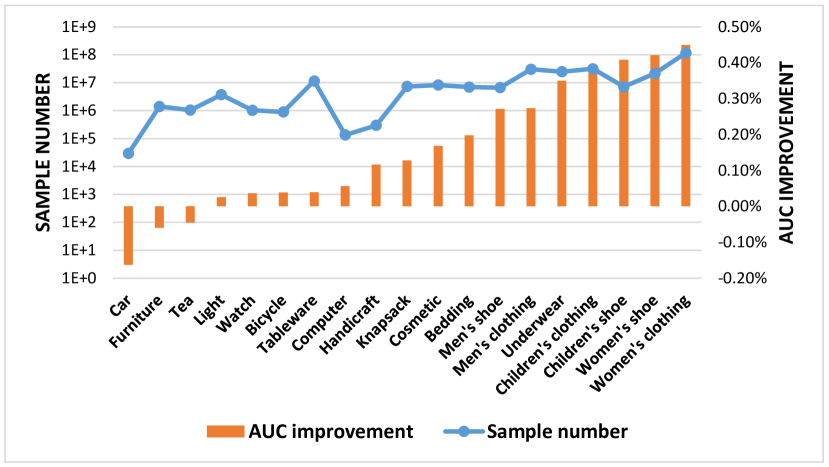
Figure 4. The AUC improvements of Courier compared to the Baseline on different categories. The x-axis is sorted by the improvements.

In Figure. 4, we plot the AUC improvements of Courier in different categories. We have the following conclusions: First, the performance improvement in the women’s clothing category is the most, which is intuitive since the embeddings are trained with women’s clothing data. Secondly, there are also significant improvements in women’s shoe, children’s shoe, children’s clothing, underwear, etc. These categories are not used in the pre-training task, which indicates the Courier method can learn general visual characteristics that reflect user interests. Thirdly, the performances in the bedding, cosmetics, knapsack, and handicrafts are also improved by more than 0.1%. These categories are significantly different from women’s clothing in visual appearance, and Courier also learned some features that are transferable to these categories. Fourthly, Courier does not have a significant impact on some categories, and has a negative impact on the car category. These categories are less influenced by visual looking and can be ignored when using our method to avoid performance drop. Fifthly, the performance is also related to the amount of data. Generally, categories that have more data tend to perform better.

4.7. Visualization of trained embeddings

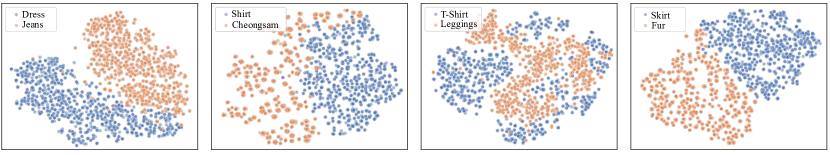
Figure 5. T-SNE visualization of embeddings in different categories.

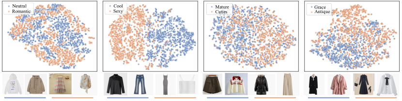
Figure 6. T-SNE visualization of embeddings with different style tags. We also plot some item images with different tags below the corresponding figures.

Did Courier really learn features related to user interests? We verified the quantitative improvements on CTR in Section. 4.5. Here, we also provide some qualitative analysis. During the training of Courier, we did not use any additional information other than images and user clicks. Thus, if the embeddings contain some semantic information, such information must be extracted from user behaviors. So we plot some randomly selected embeddings with specific categories and style tags in Figure. 5 and Figure. 6. First, embeddings from different categories are clearly separated, which indicates that Courier can learn categorical semantics from user behaviors. Secondly, some of the style tags can be separated, such as Neutral vs. Romantic, and Cool vs. Sexy. The well-separated tags are also intuitively easy to distinguish. Thirdly, some of the tags can not be separated clearly, such as Mature vs. Cuties, and Grace vs. Antique, which is also intuitive since these tags have relatively vague meanings and may overlap. Despite this, Courier still learned some gradients between the two concepts. To conclude, the proposed Courier method can learn meaningful user-interest-related features by only using images and click labels.

4.8. Influence of $\tau$

Table 4. The influence of different $\tau$.

Temperature	AUC (women’s clothing)	AUC	GAUC
0.02	0.33%	0.11%	-0.03%
0.05	0.36%	0.15%	0.09%
0.1	-0.06%	-0.31%	-0.07%
0.2	0.17%	0.07%	-0.09%

We experiment with different $\tau$. The results are in Table. (4). Note that the experiments are run with the Simscore method, which is worse than Cluster-ID but is much faster. We find that $\tau=0.05$ performs best for Courier and keep it fixed.

4.9. Ablation study

Table 5. Ablation studies of Courier.

	AUC (women’s clothing)	AUC	GAUC
w/o UCS	0.06%	-0.13%	0.11%
w/o Contrast	0.23%	0.03%	-0.11%
w/o Reconstruction	0.25%	0.02%	-0.11%
w/o Neg PV	0.30%	0.07%	-0.06%
w/o Large batch	0.15%	-0.06%	-0.08%
Courier	0.46%	0.16%	0.19%

We conduct the following ablation experiments to verify the effect of each component of Courier.

• w/o UCS: Remove the user click sequence loss.

• w/o Contrast: Remove the contrastive loss, only minimize the reconstruction loss, similar to SimSiam(Chen and He, 2021).

• w/o Reconstruction: Use self-attention instead of cross-attention in the user interest recommendation module. We further analyze this method in Appendix Section. B.

• w/o Neg PV: Remove negative PV samples, only use positive samples.

• w/o Large batch: Change batch size from 3072 to 64.

The results in Table. (5) indicate that all the proposed components are necessary for the best performance.

4.10. Train with text information

Table 6. Train with text information.

	AUC (women’s clothing)	AUC	GAUC
w CLIP	0.26%	0.04%	-0.09%
Courier	0.46%	0.16%	0.19%

Text information is important for searching and recommendation since it’s directly related to the query by the users and the properties of items. Thus, raw text information is already widely used in real-world systems. The co-train of texts and images also shows significant performance gains in computer vision tasks such as classification and segmentation. So we are interested in verifying the influence to Courier by co-training with text information. Specifically, we add a CLIP(Radford et al., 2021) besides Courier, with the loss function becomes $L=L_{\textsc{Courier}{}}+L_{CLIP}$. The CLIP loss is calculated with item cover images and item titles. However, such multi-task training leads to worse downstream CTR performance as shown in Table. (6), which indicates that co-training with the text information may not help generalization when the text information is available in the downstream task.

4.11. Deployment

Table 7. The A/B testing improvements of Courier.

	IPV	# Order	CTR	GMV
All categories	+0.11%	+0.1%	+0.18%	+0.66%
Women’s clothing	+0.26%	+0.31%	+0.34%	+0.88%

To evaluate the performance improvement brought by Courier on our online system, we conduct online A/B testing in Taobao Search for 30-days. Compared with the strongest deployed online baseline, COURIER significantly (p-value < 0.01) improves the CTR and GMV (Cross Merchandise Volume) by +0.34% and +0.88% in women’s clothing, respectively (the noise level is less than 0.1% according to the online A/A test). Such improvements are considered significant with the large volume of our Taobao search engine. The model has also been successfully deployed into production, serving the main traffic, with the Cluster-ID updated once a month.

Appendix A Downstream usage of image embeddings

How the features are fed to the model is a critical factor that affects the performance of machine learning algorithms. For example, normalizing the inputs before input to neural networks is a well-known preprocessing that matters a lot. In our practice of pre-training and utilizing pre-trained embeddings in downstream tasks, we also find that the way we insert the pre-trained embeddings is critical to the downstream performance. We explore three different approaches: Vector, Similarity score, and Cluster ID.

Vector. The most straightforward and common practices of utilizing pre-trained embeddings are to use the embeddings as input to the downstream tasks directly. In such cases, the features of the item images are represented as embedding vectors, which is also the first approach we have tried. However, our experiments show that no matter how we train the image embeddings, the improvements in the CTR task are only marginal. We think the reason is that the embedding vectors are relatively hard to be used by the downstream model, so the downstream model ignores the embedding vectors. The existing recommender systems already use item IDs as features, and the embeddings of the IDs can be trained directly. So the IDs are much easier to identify an item than image embeddings, which require multiple layers to learn to extract related information. Thus, the model will achieve high performance by updating ID embeddings before the image-related weights can learn useful representations for CTR. Then the gradient vanishes because the loss is nearly converged, and the image-related weights won’t update significantly anymore, which is also observed in our experiments.

Similarity Score. With the hypothesis about the embedding vectors, We experiment with a much-simplified representation of the embedding vectors. Specifically, assuming we want to estimate the CTR of an item with $Img_{pv}$ and a user of click history $Img_{click}^{k}$. The vector approach uses $Emb_{click}^{k}$ and $Emb_{pv}$ as inputs directly. Instead, we calculate a cosine similarity score for each click history items,

(8) $$sim(Img_{pv},Img_{click}^{k})=\frac{Img_{pv}^{T}Img_{click}^{k}}{||Img_{pv}||\;||Img_{click}^{k}||}$$

and the scores (each image corresponds to a real-valued score) are used as image features. The results are in Table. (8). Experimental results indicate that the simple similarity score features perform significantly better than inserting embedding vectors directly, although the embedding vectors contain much more information. The performance of the similarity score method verified our hypothesis that embedding vectors may be too complex to be used in the CTR task.

Table 8. Performance of inserting image information with Vector, SimScore, and Cluster ID. Since we performed this comparison in the early stage of our development, the exact configurations of each version are hard to describe in detail. And the different versions may not be comparable to each other (different training data sizes, learning rates, training methods, etc.). We only list the version number for clarity. Results within each row are comparable since they are generated from the same version of embeddings. The Baseline does not use images. "-" denotes that we did not evaluate Cluster-ID of these versions.

	Vector	SimScore	Cluster ID
Baseline	0.00%	0.00%	0.00%
V1	0.07%	0.14%	0.23%
V2	0.08%	0.16%	0.23%
V3	0.09%	0.18%	0.28%
V4	0.06%	0.16%	0.22%
V5	0.00%	0.11%	-
V6	-0.02%	0.07%	-
V7	-0.04%	-0.01%	-
V8	0.04%	0.13%	-
V9	0.05%	0.09%	-

Cluster IDs. Our experiments on embedding vectors and similarity scores indicate that embedding vectors are hard to use and simply similarity scores contain information that can improve downstream performance. Can we insert more information than similarity scores but not too much? ID features are the most important features used in recommender systems, and it has been observed that ID features are easier to train than non-ID features, and perform better(Zhang et al., 2022). Thus, we propose to transform embedding vectors into ID features. A straightforward and efficient method is to hash the embedding vectors and use the hash values as IDs. However, hashing cannot retain semantic relationships between trained embeddings, such as distances learned in contrastive learning. Thus, we propose to use the cluster IDs to represent the embedding vectors instead. Specifically, we run a clustering algorithm(Yi et al., 2014) on all the embedding vectors, then we use the ID of the nearest cluster center as the ID feature for each embedding vector. There are some benefits of using cluster IDs: First, the clustering algorithm is an efficient approximation method that are scalable to large data. Second, the cluster centers learned by the clustering algorithm have clear interpretations and retain the global and local distance structures. Third, since we are using Euclidean distance in the clustering algorithm, the learned cluster IDs can retain most of the distance information learned in the contrastive pre-training stage.

From Table. (8) we can conclude that the Cluster ID method consistently outperforms the Vector and SimScore method by a significant gap. The overall trend of SimScore and Cluster ID are similar, but evaluating with SimScore is much faster. Thus, practically we use the SimScore method to roughly compare different hyper-parameters, and the most promising hyper-parameters are further evaluated with the cluster ID method.

Why Cluster-ID is suitable for contrastive pre-training methods. The cosine similarity is related with the Euclidean distance as follows:

(9) $$Sim(\mathbf{x},\mathbf{y})=\frac{\mathbf{x}^{T}\mathbf{y}}{||\mathbf{x}||\;||\mathbf{y}||}=\frac{||\mathbf{x}||^{2}+||\mathbf{y}||^{2}-||\mathbf{x}-\mathbf{y}||^{2}}{2||\mathbf{x}||\;||\mathbf{y}||}$$

If we constrain the embedding vectors to be $\ell 2$ normalized, i.e., $||\mathbf{x}||=||\mathbf{y}||=1$, which is the same as in contrastive learning. Then we have

(10) $$Sim(\mathbf{x},\mathbf{y})=\frac{2-||\mathbf{x}-\mathbf{y}||^{2}}{2}$$

Thus, maximizing the cosine similarity is equivalent to minimizing the Euclidean distance between $\ell 2$ normalized vectors. Since we are optimizing the cosine similarity of the embedding vectors, we are indeed optimizing their Euclidean distances. And such distance information is retained by the clustering algorithm using Euclidean distances. By adjusting the number of clusters, we can also change the information to be retained. To conclude, the Cluster-ID method aligns with both the pre-training and downstream stages, resulting in better performance.

Appendix B Why not use random masked prediction and self-attention?

Random masked prediction is a popular pre-training style, which may also be applied to our framework. However, considering the data-generating process, random masking is indeed unnecessary and may cause some redundant computation and information leakage. Because of the time series nature of user click history, we will train on all the possible reconstruction targets in click history. That is, we will train with (B; A) at first, where (A) is the history and B is the target. After the user has clicked on item C, we will train on (C; B, A), and so on. Thus, every item in the click history will be treated as a target exactly once.

Suppose we adopted the random masking method, there is a chance that we train on (A; C, B), then we train on (C; A, B). Since the model has already observed the co-occurrence of A, B, and C, the next (C; A, B) prediction will be much easier. The random masking method also violates the potential causation that observing A and B causes the user’s interest in C.

Masked predictions typically use self-attention instead of cross attention with knowledge about the target as our proposed user intention reconstruction method. We also try with the self-attention method in the experiment section, which performs worse than our method. The reason is that learning to predict the next item with only a few click history is tough, but training to figure out how the next item can be reconstructed with the clicking history is much easier and can provide more meaningful signals during training.

Appendix C Does projection head help?

Table 9. Adding projection to Courier.

	AUC (women’s clothing)	AUC	GAUC
w projection	0.29%	0.06%	-0.04%
Courier	0.46%	0.16%	0.19%

Most of the contrastive pre-training methods are equipped with projection heads. A projection head refers to one or multiple layers (typically an MLP) that is appended after the last embedding layer. During training, the contrastive loss (e.g., InfoNCE) is calculated with the output of the projection head instead of using the embeddings directly. After training, the projection heads are dropped, and the embeddings are used in downstream tasks, e.g, classification. It is widely reported that training with projection heads can improve downstream performance(Chen et al., 2020a, b; Chen and He, 2021). However, the reason for the success of the projection head is still unclear. We experiment with projection heads as an extension of Courier, and the results are in Table. (9). We find that projection heads have a negative impact on Courier. There are two possible reasons: 1. In those contrastive methods, the downstream usage and the pre-training stage are inconsistent. In pre-training, the contrastive loss pushes embeddings and their augmented embeddings to be closer, which wipes away detailed information other than distance, while the distance itself cannot be used in classification. By adding projection heads, the projection head can learn the distance information without wiping away much detailed information. 2. In our Courier method, we use the distance information learned in the pre-training stage directly by calculating the similarity score or cluster ID. Thus, the contrastive loss is consistent with the downstream usage. If we train with a projection head, the embeddings are not well suited for calculating the similarity scores since the embeddings are not trained to learn cosine similarity directly.

Appendix D Implementation and Reproduction

D.1. Courier and Compared Methods

Image Backbone. We adopt the swin-tiny implementation in Torchvision. The output layer of the backbone model is replaced with a randomly initialized linear layer, and we use weights pre-trained on the ImageNet dataset to initialize other layers. We apply gradient checkpoint(Chen et al., 2016) on all the attention layers in swin-tiny to reduce memory usage and enlarge batch size. We apply half-precision (float 16) computation(Micikevicius et al., 2018) in all our models to accelerate computing and reduce memory. We train all the methods on a cluster with 48 Nvidia V100 GPUs (32GB), which enables single GPU batch size = 64, overall batch size = 64*48 = 3072. Note that each line of data contains 10 images, so the number of images within a batch is 30720 (some are padded zeros). The images are resized, cropped, and normalized before feeding to the backbone model. The input image size is 224.

We use the following hyperparameters for all the methods. Learning rate=1e-4, embedding size=256, weight decay=1e-6. We use the Adam optimizer. We have tuned these hyperparameters roughly but did not find significantly better choices on specific methods.

Hyperparameters of Courier: We use $\tau=0.05$ as reported in the paper.

Implementation of CLIP: We tune the $\tau$ within [0.1, 0.2, 0.5], and find that $\tau=0.1$ performs best, corresponding to the reported results. The batch size of CLIP is 32*48 since we have to reduce the batch size to load the language model. The effective batch size of CLIP is 32*48*5, since we only have titles of the PV items in our dataset. The text model is adapted from Chinese-BERT(Sun et al., 2021) and is initialized with the pre-trained weights provided by the authors.

Implementation of SimCLR: We tune the $\tau$ with in [0.1, 0.2, 0.5], and find that $\tau=0.2$ performs best, corresponding to the reported results. The effective batch size of SimCLR is 64*48*10. We implemented the same augmentation strategy as suggested by the SimCLR paper(Chen et al., 2020a).

Implementation of SimSiam: The effective batch size of SimSiam is 64*48*10. The augmentation method is the same as SimCLR.

D.2. Code and Data

We provide the main codes for implementing our Courier method at https://anonymous.4open.science/r/COURIER/ for review, which will be open-sourced once accepted to support potential usage on other datasets. Some parts of our code extensively use our internal tools and involve our private data processing, so we delete the sensitive codes. Our dataset contains sensitive personal information from users that can not be published in any form.

References

- (1)
- An et al. (2019) Mingxiao An, Fangzhao Wu, Chuhan Wu, Kun Zhang, Zheng Liu, and Xing Xie. 2019. Neural News Recommendation with Long- and Short-term User Representations. In ACL. Association for Computational Linguistics, 336–345. https://doi.org/10.18653/v1/p19-1033
- Anonymous (2023) Anonymous. 2023. Where to Go Next for Recommender Systems? ID- vs. Modality-based recommender models revisited. In Submitted to The Eleventh International Conference on Learning Representations. https://openreview.net/forum?id=bz3MAU-RhnW under review.
- Bi et al. (2022) Qiwei Bi, Jian Li, Lifeng Shang, Xin Jiang, Qun Liu, and Hanfang Yang. 2022. MTRec: Multi-Task Learning over BERT for News Recommendation. In ACL Findings. Association for Computational Linguistics, 2663–2669. https://doi.org/10.18653/v1/2022.findings-acl.209
- Brown et al. (2020) Tom B. Brown, Benjamin Mann, Nick Ryder, Melanie Subbiah, Jared Kaplan, Prafulla Dhariwal, Arvind Neelakantan, Pranav Shyam, Girish Sastry, Amanda Askell, Sandhini Agarwal, Ariel Herbert-Voss, Gretchen Krueger, Tom Henighan, Rewon Child, Aditya Ramesh, Daniel M. Ziegler, Jeffrey Wu, Clemens Winter, Christopher Hesse, Mark Chen, Eric Sigler, Mateusz Litwin, Scott Gray, Benjamin Chess, Jack Clark, Christopher Berner, Sam McCandlish, Alec Radford, Ilya Sutskever, and Dario Amodei. 2020. Language Models are Few-Shot Learners. In NeurIPS.
- Chen et al. (2020a) Ting Chen, Simon Kornblith, Mohammad Norouzi, and Geoffrey E. Hinton. 2020a. A Simple Framework for Contrastive Learning of Visual Representations. In ICML (Proceedings of Machine Learning Research, Vol. 119). PMLR, 1597–1607.
- Chen et al. (2020b) Ting Chen, Simon Kornblith, Kevin Swersky, Mohammad Norouzi, and Geoffrey E. Hinton. 2020b. Big Self-Supervised Models are Strong Semi-Supervised Learners. In NeurIPS.
- Chen et al. (2016) Tianqi Chen, Bing Xu, Chiyuan Zhang, and Carlos Guestrin. 2016. Training Deep Nets with Sublinear Memory Cost. CoRR abs/1604.06174 (2016). arXiv:1604.06174
- Chen and He (2021) Xinlei Chen and Kaiming He. 2021. Exploring Simple Siamese Representation Learning. In CVPR. Computer Vision Foundation / IEEE, 15750–15758. https://doi.org/10.1109/CVPR46437.2021.01549
- Covington et al. (2016) Paul Covington, Jay Adams, and Emre Sargin. 2016. Deep Neural Networks for YouTube Recommendations. In RecSys. ACM, 191–198. https://doi.org/10.1145/2959100.2959190
- Deng et al. (2009) Jia Deng, Wei Dong, Richard Socher, Li-Jia Li, Kai Li, and Li Fei-Fei. 2009. ImageNet: A large-scale hierarchical image database. In CVPR. IEEE Computer Society, 248–255. https://doi.org/10.1109/CVPR.2009.5206848
- Devlin et al. (2019) Jacob Devlin, Ming-Wei Chang, Kenton Lee, and Kristina Toutanova. 2019. BERT: Pre-training of Deep Bidirectional Transformers for Language Understanding. In NAACL-HLT. Association for Computational Linguistics, 4171–4186. https://doi.org/10.18653/v1/n19-1423
- Ding et al. (2021) Hao Ding, Yifei Ma, Anoop Deoras, Yuyang Wang, and Hao Wang. 2021. Zero-Shot Recommender Systems. CoRR abs/2105.08318 (2021). arXiv:2105.08318
- Dong et al. (2022) Xiao Dong, Xunlin Zhan, Yangxin Wu, Yunchao Wei, Michael C. Kampffmeyer, Xiaoyong Wei, Minlong Lu, Yaowei Wang, and Xiaodan Liang. 2022. M5Product: Self-harmonized Contrastive Learning for E-commercial Multi-modal Pretraining. In CVPR. IEEE, 21220–21230. https://doi.org/10.1109/CVPR52688.2022.02057
- Elsayed et al. (2022) Shereen Elsayed, Lukas Brinkmeyer, and Lars Schmidt-Thieme. 2022. End-to-End Image-Based Fashion Recommendation. CoRR abs/2205.02923 (2022). https://doi.org/10.48550/arXiv.2205.02923 arXiv:2205.02923
- Feng et al. (2019) Yufei Feng, Fuyu Lv, Weichen Shen, Menghan Wang, Fei Sun, Yu Zhu, and Keping Yang. 2019. Deep Session Interest Network for Click-Through Rate Prediction. In IJCAI, Sarit Kraus (Ed.). ijcai.org, 2301–2307. https://doi.org/10.24963/ijcai.2019/319
- Grill et al. (2020) Jean-Bastien Grill, Florian Strub, Florent Altché, Corentin Tallec, Pierre H. Richemond, Elena Buchatskaya, Carl Doersch, Bernardo Ávila Pires, Zhaohan Guo, Mohammad Gheshlaghi Azar, Bilal Piot, Koray Kavukcuoglu, Rémi Munos, and Michal Valko. 2020. Bootstrap Your Own Latent - A New Approach to Self-Supervised Learning. In NeurIPS.
- He and McAuley (2016) Ruining He and Julian J. McAuley. 2016. Ups and Downs: Modeling the Visual Evolution of Fashion Trends with One-Class Collaborative Filtering. In WWW. ACM, 507–517. https://doi.org/10.1145/2872427.2883037
- He et al. (2017) Xiangnan He, Lizi Liao, Hanwang Zhang, Liqiang Nie, Xia Hu, and Tat-Seng Chua. 2017. Neural Collaborative Filtering. In WWW. ACM, 173–182. https://doi.org/10.1145/3038912.3052569
- Hidasi et al. (2016) Balázs Hidasi, Alexandros Karatzoglou, Linas Baltrunas, and Domonkos Tikk. 2016. Session-based Recommendations with Recurrent Neural Networks. In ICLR.
- Hou et al. (2019) Min Hou, Le Wu, Enhong Chen, Zhi Li, Vincent W. Zheng, and Qi Liu. 2019. Explainable Fashion Recommendation: A Semantic Attribute Region Guided Approach. In IJCAI. ijcai.org, 4681–4688. https://doi.org/10.24963/ijcai.2019/650
- Hou et al. (2022) Yupeng Hou, Shanlei Mu, Wayne Xin Zhao, Yaliang Li, Bolin Ding, and Ji-Rong Wen. 2022. Towards Universal Sequence Representation Learning for Recommender Systems. In KDD. ACM, 585–593. https://doi.org/10.1145/3534678.3539381
- Huang et al. (2013) Po-Sen Huang, Xiaodong He, Jianfeng Gao, Li Deng, Alex Acero, and Larry P. Heck. 2013. Learning deep structured semantic models for web search using clickthrough data. In CIKM. ACM, 2333–2338. https://doi.org/10.1145/2505515.2505665
- Koren et al. (2009) Yehuda Koren, Robert M. Bell, and Chris Volinsky. 2009. Matrix Factorization Techniques for Recommender Systems. Computer 42, 8 (2009), 30–37. https://doi.org/10.1109/MC.2009.263
- Lee and Abu-El-Haija (2017) Joonseok Lee and Sami Abu-El-Haija. 2017. Large-Scale Content-Only Video Recommendation. In ICCV Workshops. IEEE Computer Society, 987–995. https://doi.org/10.1109/ICCVW.2017.121
- Lei et al. (2021) Chenyi Lei, Yong Liu, Lingzi Zhang, Guoxin Wang, Haihong Tang, Houqiang Li, and Chunyan Miao. 2021. SEMI: A Sequential Multi-Modal Information Transfer Network for E-Commerce Micro-Video Recommendations. In KDD. ACM, 3161–3171. https://doi.org/10.1145/3447548.3467189
- Li et al. (2022) Jian Li, Jieming Zhu, Qiwei Bi, Guohao Cai, Lifeng Shang, Zhenhua Dong, Xin Jiang, and Qun Liu. 2022. MINER: Multi-Interest Matching Network for News Recommendation. In ACL Findings. Association for Computational Linguistics, 343–352. https://doi.org/10.18653/v1/2022.findings-acl.29
- Linden et al. (2003) Greg Linden, Brent Smith, and Jeremy York. 2003. Amazon.com Recommendations: Item-to-Item Collaborative Filtering. IEEE Internet Comput. 7, 1 (2003), 76–80. https://doi.org/10.1109/MIC.2003.1167344
- Liu et al. (2021a) Zhiwei Liu, Yongjun Chen, Jia Li, Philip S. Yu, Julian J. McAuley, and Caiming Xiong. 2021a. Contrastive Self-supervised Sequential Recommendation with Robust Augmentation. CoRR abs/2108.06479 (2021). arXiv:2108.06479 https://arxiv.org/abs/2108.06479
- Liu et al. (2021b) Ze Liu, Yutong Lin, Yue Cao, Han Hu, Yixuan Wei, Zheng Zhang, Stephen Lin, and Baining Guo. 2021b. Swin Transformer: Hierarchical Vision Transformer using Shifted Windows. In ICCV. IEEE, 9992–10002. https://doi.org/10.1109/ICCV48922.2021.00986
- Liu et al. (2021c) Zhuang Liu, Yunpu Ma, Yuanxin Ouyang, and Zhang Xiong. 2021c. Contrastive Learning for Recommender System. CoRR abs/2101.01317 (2021). arXiv:2101.01317 https://arxiv.org/abs/2101.01317
- McAuley et al. (2015) Julian J. McAuley, Christopher Targett, Qinfeng Shi, and Anton van den Hengel. 2015. Image-Based Recommendations on Styles and Substitutes. In SIGIR. ACM, 43–52. https://doi.org/10.1145/2766462.2767755
- Micikevicius et al. (2018) Paulius Micikevicius, Sharan Narang, Jonah Alben, Gregory F. Diamos, Erich Elsen, David García, Boris Ginsburg, Michael Houston, Oleksii Kuchaiev, Ganesh Venkatesh, and Hao Wu. 2018. Mixed Precision Training. In ICLR. OpenReview.net.
- Mustafa et al. (2022) Basil Mustafa, Carlos Riquelme Ruiz, Joan Puigcerver, Rodolphe Jenatton, and Neil Houlsby. 2022. Multimodal Contrastive Learning with LIMoE: the Language-Image Mixture of Experts. In Advances in Neural Information Processing Systems, Alice H. Oh, Alekh Agarwal, Danielle Belgrave, and Kyunghyun Cho (Eds.).
- Poole et al. (2019) Ben Poole, Sherjil Ozair, Aäron van den Oord, Alexander A. Alemi, and George Tucker. 2019. On Variational Bounds of Mutual Information. In ICML (Proceedings of Machine Learning Research, Vol. 97). PMLR, 5171–5180.
- Qiu et al. (2022) Ruihong Qiu, Zi Huang, Hongzhi Yin, and Zijian Wang. 2022. Contrastive Learning for Representation Degeneration Problem in Sequential Recommendation. In WSDM. ACM, 813–823. https://doi.org/10.1145/3488560.3498433
- Radford et al. (2021) Alec Radford, Jong Wook Kim, Chris Hallacy, Aditya Ramesh, Gabriel Goh, Sandhini Agarwal, Girish Sastry, Amanda Askell, Pamela Mishkin, Jack Clark, Gretchen Krueger, and Ilya Sutskever. 2021. Learning Transferable Visual Models From Natural Language Supervision. In ICML (Proceedings of Machine Learning Research, Vol. 139). PMLR, 8748–8763.
- Schafer et al. (2007) J. Ben Schafer, Dan Frankowski, Jonathan L. Herlocker, and Shilad Sen. 2007. Collaborative Filtering Recommender Systems. In The Adaptive Web, Methods and Strategies of Web Personalization (Lecture Notes in Computer Science, Vol. 4321). Springer, 291–324. https://doi.org/10.1007/978-3-540-72079-9_9
- Su et al. (2020) Weijie Su, Xizhou Zhu, Yue Cao, Bin Li, Lewei Lu, Furu Wei, and Jifeng Dai. 2020. VL-BERT: Pre-training of Generic Visual-Linguistic Representations. In ICLR. OpenReview.net.
- Sun et al. (2019) Fei Sun, Jun Liu, Jian Wu, Changhua Pei, Xiao Lin, Wenwu Ou, and Peng Jiang. 2019. BERT4Rec: Sequential Recommendation with Bidirectional Encoder Representations from Transformer. In CIKM. ACM, 1441–1450. https://doi.org/10.1145/3357384.3357895
- Sun et al. (2021) Zijun Sun, Xiaoya Li, Xiaofei Sun, Yuxian Meng, Xiang Ao, Qing He, Fei Wu, and Jiwei Li. 2021. ChineseBERT: Chinese Pretraining Enhanced by Glyph and Pinyin Information. In ACL/IJCNLP. Association for Computational Linguistics, 2065–2075. https://doi.org/10.18653/v1/2021.acl-long.161
- van den Oord et al. (2013) Aäron van den Oord, Sander Dieleman, and Benjamin Schrauwen. 2013. Deep content-based music recommendation. In NIPS. 2643–2651.
- Vaswani et al. (2017) Ashish Vaswani, Noam Shazeer, Niki Parmar, Jakob Uszkoreit, Llion Jones, Aidan N. Gomez, Lukasz Kaiser, and Illia Polosukhin. 2017. Attention is All you Need. In NIPS. 5998–6008.
- Wang et al. (2022a) Fangye Wang, Yingxu Wang, Dongsheng Li, Hansu Gu, Tun Lu, Peng Zhang, and Ning Gu. 2022a. CL4CTR: A Contrastive Learning Framework for CTR Prediction. CoRR abs/2212.00522 (2022). https://doi.org/10.48550/arXiv.2212.00522 arXiv:2212.00522
- Wang et al. (2022b) Jie Wang, Fajie Yuan, Mingyue Cheng, Joemon M. Jose, Chenyun Yu, Beibei Kong, Zhijin Wang, Bo Hu, and Zang Li. 2022b. TransRec: Learning Transferable Recommendation from Mixture-of-Modality Feedback. CoRR abs/2206.06190 (2022). https://doi.org/10.48550/arXiv.2206.06190 arXiv:2206.06190
- Wang and Wang (2014) Xinxi Wang and Ye Wang. 2014. Improving Content-based and Hybrid Music Recommendation using Deep Learning. In ACM MM. ACM, 627–636. https://doi.org/10.1145/2647868.2654940
- Wei et al. (2019) Yinwei Wei, Xiang Wang, Liqiang Nie, Xiangnan He, Richang Hong, and Tat-Seng Chua. 2019. MMGCN: Multi-modal Graph Convolution Network for Personalized Recommendation of Micro-video. In ACM MM. ACM, 1437–1445. https://doi.org/10.1145/3343031.3351034
- Wu et al. (2021b) Chuhan Wu, Fangzhao Wu, Tao Qi, and Yongfeng Huang. 2021b. Empowering News Recommendation with Pre-trained Language Models. In SIGIR. ACM, 1652–1656. https://doi.org/10.1145/3404835.3463069
- Wu et al. (2021a) Jiancan Wu, Xiang Wang, Fuli Feng, Xiangnan He, Liang Chen, Jianxun Lian, and Xing Xie. 2021a. Self-supervised Graph Learning for Recommendation. In SIGIR. ACM, 726–735. https://doi.org/10.1145/3404835.3462862
- Wu et al. (2020) Le Wu, Lei Chen, Richang Hong, Yanjie Fu, Xing Xie, and Meng Wang. 2020. A Hierarchical Attention Model for Social Contextual Image Recommendation. IEEE Trans. Knowl. Data Eng. 32, 10 (2020), 1854–1867. https://doi.org/10.1109/TKDE.2019.2913394
- Xiao et al. (2022) Shitao Xiao, Zheng Liu, Yingxia Shao, Tao Di, Bhuvan Middha, Fangzhao Wu, and Xing Xie. 2022. Training Large-Scale News Recommenders with Pretrained Language Models in the Loop. In KDD. ACM, 4215–4225. https://doi.org/10.1145/3534678.3539120
- Xie et al. (2022) Xu Xie, Fei Sun, Zhaoyang Liu, Shiwen Wu, Jinyang Gao, Jiandong Zhang, Bolin Ding, and Bin Cui. 2022. Contrastive Learning for Sequential Recommendation. In ICDE. IEEE, 1259–1273. https://doi.org/10.1109/ICDE53745.2022.00099
- Yao et al. (2021) Tiansheng Yao, Xinyang Yi, Derek Zhiyuan Cheng, Felix X. Yu, Ting Chen, Aditya Krishna Menon, Lichan Hong, Ed H. Chi, Steve Tjoa, Jieqi (Jay) Kang, and Evan Ettinger. 2021. Self-supervised Learning for Large-scale Item Recommendations. In CIKM. ACM, 4321–4330. https://doi.org/10.1145/3459637.3481952
- Yi et al. (2014) Jinfeng Yi, Lijun Zhang, Jun Wang, Rong Jin, and Anil K. Jain. 2014. A Single-Pass Algorithm for Efficiently Recovering Sparse Cluster Centers of High-dimensional Data. In ICML (JMLR Workshop and Conference Proceedings, Vol. 32). JMLR.org, 658–666.
- Zhang et al. (2019) Shuai Zhang, Lina Yao, Aixin Sun, and Yi Tay. 2019. Deep Learning Based Recommender System: A Survey and New Perspectives. ACM Comput. Surv. 52, 1 (2019), 5:1–5:38. https://doi.org/10.1145/3285029
- Zhang et al. (2021) Weinan Zhang, Jiarui Qin, Wei Guo, Ruiming Tang, and Xiuqiang He. 2021. Deep Learning for Click-Through Rate Estimation. In IJCAI. ijcai.org, 4695–4703. https://doi.org/10.24963/ijcai.2021/636
- Zhang et al. (2022) Zhao-Yu Zhang, Xiang-Rong Sheng, Yujing Zhang, Biye Jiang, Shuguang Han, Hongbo Deng, and Bo Zheng. 2022. Towards Understanding the Overfitting Phenomenon of Deep Click-Through Rate Models. In CIKM. ACM, 2671–2680. https://doi.org/10.1145/3511808.3557479
- Zhou et al. (2019) Guorui Zhou, Na Mou, Ying Fan, Qi Pi, Weijie Bian, Chang Zhou, Xiaoqiang Zhu, and Kun Gai. 2019. Deep Interest Evolution Network for Click-Through Rate Prediction. In AAAI. AAAI Press, 5941–5948. https://doi.org/10.1609/aaai.v33i01.33015941
- Zhou et al. (2020) Kun Zhou, Hui Wang, Wayne Xin Zhao, Yutao Zhu, Sirui Wang, Fuzheng Zhang, Zhongyuan Wang, and Ji-Rong Wen. 2020. S3-Rec: Self-Supervised Learning for Sequential Recommendation with Mutual Information Maximization. In CIKM. ACM, 1893–1902. https://doi.org/10.1145/3340531.3411954