Effects of quantum fluctuations on macroscopic quantum tunneling and self- trapping of BEC in a double well trap

Abstract

We study the influence of quantum fluctuations on the macroscopic quantum tunneling and self-trapping of a two-component Bose-Einstein condensate in a double-well trap. Quantum fluctuations are described by the Lee-Huang-Yang term in the modified Gross-Pitaevskii equation. Employing the modified Gross-Pitaevskii equation in scalar approximation, we derive the dimer model using a two-mode approximation. The frequencies of Josephson oscillations and self-trapping conditions under quantum fluctuations are found analytically and proven by numerical simulations of the modified Gross-Pitaevskii equation. The tunneling and localization phenomena are investigated also for the case of the Lee-Huang-Yang fluid loaded in the double-well potential.

1 Introduction

Recently much attention has been paid to the study of the beyond mean-field effects. The contribution to the energy of a BEC due to quantum fluctuations around the Bogolyubov ground state has been found by Lee, Huang and Yang (LHY) [1]. While these corrections are small, in many cases they lead to nontrivial effects. One of important is their role in the collapsing condensate. It has been shown, that in the case of two-component condensate, quantum fluctuations(QF) can stabilize collapsing regime and lead to the appearance of quantum droplets(QD) [2, 3]. Generation of the quantum droplets in the Bose mixture is possible due to the joint action of the attractive residual mean-field interaction and the effective repulsion introduced by QF. Another system is a dipolar BEC, where quantum droplets are generated by the balance between the small residual mean-field attraction of a combination of local two-body interactions, repulsive dipolar interactions and repulsive LHY term [5]. The existence of QD in other systems as the Bose-Fermi mixtures and Rabi-coupled BEC is discussed in works [6, 7].

The influence of the beyond mean-field (BMF) contribution has been studied for the collective excitations spectrum in Ref. [9],while modulational instability of matter waves has been studied in Ref. [10].

In this regard, it is interesting to study the influence of BMF contribution to another phenomena in the BEC. An important case is the processes of macroscopic quantum tunneling (MQT) and self-trapping(ST) in BEC loaded in a double-well trap potential. In this system, the nonlinearity due to the interaction between atoms plays an important role. In particular, it induces the transition from the Josephson oscillations(JO) of atomic imbalance to the nonlinear self-trapping (ST) regime [12]. The quantum fluctuations induce an additional nonlinear interaction in the form of effective repulsion. Thus in some region of parameters, we can expect the processes of tunneling in the double-well potential to be very sensitive to the action of quantum fluctuations. In this problem, we have a few small parameters: the tunneling parameter(describing the amplitude of tunneling between condensates), the strength of QF given by the LHY correction, and the residual mean field nonlinearity between components of BEC. When they are comparable, we can expect new regimes in the switching of the matter waves in the double-well potential. The important limiting case of the vanishing of residual mean-field interactions is a LHY fluid [11] loaded in the double-well potential. Note that recently the LHY fluid has been observed in Ref.  [13]

In this work, we study the MQT and ST processes in a two-component quasi-one-dimensional BEC loaded into a double-well trap, when quantum fluctuations are taken into account.

The structure of the paper is as follows.

In Section 2, we describe the modified quasi-one-dimensional GP equation, obtained for two-component BEC in a scalar approximation and including the LHY term. In Section 3, two-mode(dimer) model for BEC loaded into the double-well trap is derived. The Hamiltonian, fixed points, the Josephson oscillations are analyzed in Section 4. The nonlinear self-trapped regime is discussed in Section 4.2. In Section 5, results of full numerical simulations of the modified Gross-Pitaevskii(GP) equation with the double-well potential are presented. The conditions for experimental observation of the investigated effects are discussed.

2 The beyond mean field model for a BEC in a double-well potential

We consider the dynamics of a two-component BEC loaded in a cigar-type trap, when the beyond mean-field effects, describing quantum fluctuations, are taken into account. Assuming that the wave functions are related by:

$$\Psi_{1}=\sqrt{\frac{g_{11}}{g_{22}}}\Psi_{2}=\Psi,$$

where $g_{ij}=4\pi\hbar^{2}a_{ij}/m$, $a_{ij}$ are inter- and intra-species atomic scattering lengths, and supposing $g_{11}=g_{22}=g$ and $g_{12}=\delta g+g$, we reduce the coupled GP equations to the scalar GP equation for $\Psi$. Then the governing equation, describing the wave function of a condensate with the Lee-Huang-Yang term, is [2]:

$$i\hbar\Psi_{t}(r,t)=-\frac{\hbar^{2}}{2m}\nabla^{2}\Psi(r,t)+V(r)\Psi(r,t)-\delta g|\Psi|^{2}\Psi+\gamma_{LHY}|\Psi|^{3}\Psi,$$ (1)

where

$$\gamma_{LHY}=\frac{128\sqrt{\pi}\hbar^{2}}{3m}|a|^{5/2}.$$

We study below a quasi-one-dimensional geometry given by a cigar-type trap, when the transversal ($\omega_{\perp}$) and longitudinal ($\omega_{x}$) trap frequencies are satisfied to the condition $\omega_{\perp}\gg\omega_{x}$. Here we use the factorization [14]:

$$\Psi=\Phi(x,t)R(\rho),\ R(\rho)=Ae^{-\rho^{2}/2l_{\perp}^{2}},\ l_{\perp}=\sqrt{\hbar/(m\omega_{\perp})}.\$$ (2)

After integration over the transverse distribution, we obtain the quasi-one-dimensional MGP equation:

$$i\hbar\Psi_{t}(x,t)=-\frac{\hbar^{2}}{2m}\Psi_{xx}(x,t)+V(x)_{ext}\Psi(x,t)-\frac{\delta g}{2\pi l_{\perp}^{2}}|\Psi|^{2}\Psi+\frac{2\gamma_{LHY}}{5\pi^{3/2}l_{\perp}^{3}}|\Psi|^{3}\Psi,$$ (3)

where $V_{ext}(x)$ is a double well potential chosen as

$$V_{ext}(x)=\frac{mw_{x}^{2}}{2}x^{2}+U_{0}\exp(-(x/l_{0})^{2}).$$ (4)

It is useful to introduce dimensionless variables according to:

$$t=\omega_{x}t,x=\frac{x}{l_{x}},\ l_{x}=\sqrt{\frac{\hbar}{m\omega_{x}}},\psi=\sqrt{\frac{l_{x}}{N}}\psi.$$

Then we can rewrite the governing equation as follows:

$$i\psi_{t}=-\frac{1}{2}\psi_{xx}+V_{ext}(x)\psi+\delta g|\psi|^{2}\psi+\gamma|\psi|^{3}\psi,$$ (5)

where

$$\delta g=\frac{4\delta a}{l_{x}}\frac{\omega_{\perp}}{\omega_{x}}N,\gamma=\frac{128}{15\pi}(\frac{a}{l_{x}})^{5/2}(\frac{\omega_{\perp}}{\omega_{x}})^{3/2}N^{3/2},$$

$$V_{ext}=\frac{1}{2}x^{2}+V_{0}e^{-(x/l)^{2}},l=\frac{l_{0}}{l_{x}},V_{0}=\frac{U_{0}}{\hbar\omega_{x}}.$$

This normalization of the wave function $\psi$ corresponds to:

$$\int_{-\infty}^{\infty}|\psi|^{2}dx=1.$$

Let us estimate the parameters for the experiments, as performed in Ref.[13]. The atomic scattering length is about $100a_{0}$, where $a_{0}$ is the Bohr radius, $l_{x}\approx 300\mu m$, $N=10^{2}\div 10^{3}$. The values of parameters $g=0\div 10,\ \gamma=0.01\div 1$.

3 Two-mode model

To describe the dynamics of the BEC we will use the two-mode model [12]. Let us consider the solution in the form:

$$\psi=u(t)\Phi_{1}(x)+v(t)\Phi_{2}(x),$$ (6)

where $\Phi_{1,2}(x)$ are determined by the solutions of the stationary GP equation. Firstly we obtain two solutions of the stationary equation, (ground state with the norm $N_{gr}=1$ and an excited state with the same norm $N_{exc}=1$)

$$[-\frac{1}{2}\frac{d^{2}}{dx^{2}}+V_{ext}(x)+\delta g|\Phi_{gr/exc}|^{2}+$$

$$\gamma|\Phi_{gr/exc}|^{3}-\mu]\Phi_{gr/exc}=0.$$ (7)

It should be noted that a ground state function and an excited one are chosen to be symmetric and antisymmetric, respectively, $\Phi_{gr}(-x)=\Phi_{gr}(x)$ and $\Phi_{exc}(-x)=-\Phi_{exc}(x)$. Then, functions $\Phi_{1,2}(x)$, localized in corresponding wells (1,2) of the double-well potential are expressed as

$$\Phi_{1}(x)=(\Phi_{gr}(x)+\Phi_{exc}(x))/\sqrt{2},$$ (8)

$$\Phi_{2}(x)=(\Phi_{gr}(x)-\Phi_{exc}(x))/\sqrt{2},$$ (9)

$$I=\int_{-\infty}^{\infty}\Phi_{i}(x)\Phi_{j}(x)dx,\ i,j=1,2.$$ (10)

where $I$ is the overlap integral.

In Fig. 1 the double-well potential with wave functions $\Phi_{1,2}(x)$ are depicted. Note that the two-mode approximation works well for the small mean field nonlinearity and overlaps [15, 16]

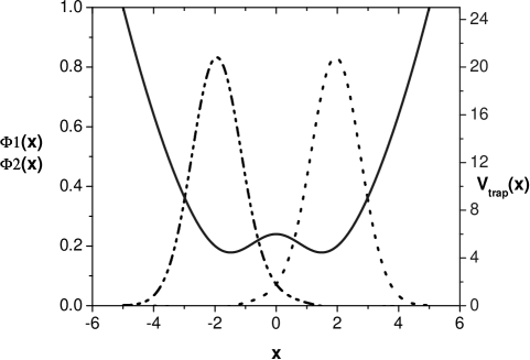
Figure 1: The double-well potential with parameters $V_{0}=5,\ l=1.5$. The solid line is for the double-well potential, - dash-dot-dot and dot- lines are for $\Phi_{2}(x)$ and $\Phi_{1}(x)$ wave functions, respectively.

Let us substitute the solution  6 into Eq. (3), and multiply by $\Phi_{1}$, and integrate over $x$ in the interval $(-\infty,+\infty)$. Supposing a weak overlap criterion and ignoring nonlinear overlap integrals, we obtain the following equation:

$$iu_{t}=E_{1}^{0}u-Kv-\alpha|u|^{2}u+\beta|u|^{3}u.$$ (11)

In a similar way, the equation for $v(t)$ can be obtained

$$iv_{t}=E_{2}^{0}v-Ku-\alpha|v|^{2}v+\beta|v|^{3}v.$$ (12)

Here $E_{1,2}^{0}$ are the zero-point energies in each well, for the symmetric trap $E_{1}^{0}=E_{2}^{0}$. K is the amplitude of the tunneling, $\alpha$ and $\beta$ are other nonlinearity parameters

$$E_{1}^{0}=\frac{1}{2}\int_{-\infty}^{\infty}|\Phi_{1,x}|^{2}dx+\int_{-\infty}^{\infty}\Phi_{1}V(x)\Phi_{1}dx,$$ (13)

$$K=-\left(\frac{1}{2}\int_{-\infty}^{\infty}\Phi_{1,x}\Phi_{2,x}dx+\int_{-\infty}^{\infty}\Phi_{1}V(x)\Phi_{2}dx\right),$$ (14)

$$\alpha=\delta g\int|\Phi_{1}|^{4}dx,\ \beta=\gamma\int\Phi_{1}^{5}dx.$$ (15)

The condition of the applicability of the two-mode model is $\mu<V_{0}$, where $\mu$ is the chemical potential. For more details see the work  [15], where the different extensions of the two-mode model are considered.

4 Dimer model with LHY terms

We consider below the symmetric dimer case, when $\Delta E=E_{1}^{0}-E_{2}^{0}=0$. Then eqs.(11),(12) are written as:

$$iu_{t}+Kv+\alpha|u|^{2}u-\beta|u|^{3}u-E_{1}^{0}u=0,$$ (16)

$$iv_{t}+Ku+\alpha|v|^{2}v-\beta|v|^{3}v-E_{1}^{0}v=0.$$ (17)

Introducing variables:

$$u=\sqrt{N_{1}}e^{i\phi_{1}},\ v=\sqrt{N_{2}}e^{i\phi_{2}},$$

we obtain coupled equations for the relative imbalance $Z=(N_{1}-N_{2})/N$ and the relative phase $\psi=\phi_{2}-\phi_{1}$:

$$Z_{t}=-2K\sqrt{1-Z^{2}}\sin{\psi},$$ (18)

$$\psi_{t}=2K\frac{Z}{\sqrt{1-Z^{2}}}\cos{\psi}+\alpha NZ-\frac{\beta N^{3/2}}{2^{3/2}}[(1+Z)^{3/2}-(1-Z)^{3/2}].$$ (19)

Introducing variables:

$$\Lambda=\frac{\alpha N}{2K},\ \epsilon=\frac{\beta N^{3/2}}{2K},\ t=2Kt,$$

we get:

$$Z_{t}=-\sqrt{1-Z^{2}}\sin{\psi},$$ (20)

$$\psi_{t}=\frac{Z}{\sqrt{1-Z^{2}}}\cos{\psi}+\Lambda Z-\frac{\epsilon}{2^{3/2}}[(1-Z)^{3/2}-(1+Z)^{3/2}].$$ (21)

This system has the Hamiltonian form:

$$Z_{t}=-\frac{\partial H}{\partial\phi},\ \psi_{t}=\frac{\partial H}{\partial Z},$$ (22)

with the Hamiltonian

$$H=-\sqrt{1-Z^{2}}\cos{\psi}+\frac{\Lambda}{2}Z^{2}+\frac{\epsilon}{5\sqrt{2}}a,$$ (23)

where

$$a=[(1+Z)^{5/2}+(1-Z)^{5/2}].$$

The case, when the residual mean field interaction is equal to zero,$\Lambda=0$, corresponds to the Lee-Huang-Yang fluid, loaded into a double-well potential [11].

4.1 Josephson oscillations

To analyze different regimes in the dynamics of the atomic population imbalance and the relative phase, let us find the stationary states of the system. Equating the derivatives on time to zero, we have:

$$\psi_{c}=2\pi n,\ z_{c}=0,n=0,1,2,...\ \mbox{with}\ E_{+}=-1+\frac{\sqrt{2}}{5}\epsilon,$$

and

$$\psi_{c}=(2n+1)\pi,\ z_{c}=0,n=0,1,2,...\ \mbox{with}\ E_{-}=1+\frac{\sqrt{2}}{5}\epsilon,$$

where $E_{+/-}$ are the values of Hamiltonian  (23) at the critical points $Z_{c},\ \psi_{c}$. From Eq. (22), we can find the frequencies of Josephson oscillations $\omega_{J}$ of the atomic population imbalance $Z$. Two cases of the relative phase difference can be studied.

i).The case of a zero-phase mode: $\psi(0)=0,<Z>=0$. Then we obtain for the frequency of small oscillations Z, i.e. the JO frequency $\omega_{J}$:

$$\omega_{J}=\sqrt{1+\Lambda+\frac{3\sqrt{2}\epsilon}{4}}.$$ (24)

ii).The case of a $\pi$-phase mode: $\psi(0)=\pi,\ <z>=0.$ The frequency of the JO is:

$$\omega_{J}=\sqrt{1-\Lambda-\frac{3\sqrt{2}\epsilon}{4}}.$$ (25)

If the strength of the residual mean field nonlinearity and the LHY corrections are satisfied to the relation:

$$\Lambda=-\frac{3\sqrt{2}\epsilon}{4},\ \alpha=\frac{3\beta N^{1/2}}{2^{3/2}},$$ (26)

then the frequency of Josephson oscillations is close to the frequency of oscillations of the unperturbed system (the Rabi oscillations case). It corresponds to the quasi-linear regime. Thus it is open the possibility to measure the strength of quantum fluctuations strength by properly detuning the residual mean-field scattering length $\delta a=-|a_{12}|+a.$

If we linearize Eq. (22) on $Z$ only, the next equation for the phase is obtained:

$$\psi_{tt}+(\Lambda+\frac{3\epsilon}{2^{3/2}})\sin(\psi)+\frac{1}{2}\sin(2\psi)=0.$$ (27)

This equation has the form of an equation of motion of the unit mass particle under the action of the periodic potential. When $\epsilon=0$, the result obtained in Ref. [12] is reproduced. At $\psi=\pi$($\pi$-phase mode), in the potential a valley exists, where the effective particle oscillates. By properly detuning the parameter $\Lambda\rightarrow 1-3\epsilon/2^{3/2}$, we can diminish this valley to zero. The nonlinearity breaks the $z$-symmetry and leads to the appearance of states with $\langle Z\rangle\neq 0$.

4.2 Self-trapped regime

The self-trapped regime corresponds to the localization of atoms in one of the wells, i.e. to $\langle Z\rangle\neq 0$. If the population imbalance is fixed, then we can obtain the condition on the nonlinearity parameter. It can be find from the condition:

$$H>1+\frac{\sqrt{2}\epsilon}{5}.$$ (28)

Using Eq. (23), we obtain the condition for self-trapping:

$$\Lambda>\Lambda_{c}=\frac{2}{Z(0)^{2}}[1+\frac{\epsilon}{5\sqrt{2}}(2-a)+\sqrt{1-Z(0)^{2}}\cos(\psi(0))].$$ (29)

For the LHY fluid case, the localization criterion is:

$$\epsilon_{c}=\frac{5\sqrt{2}(1+\sqrt{1-Z(0)^{2}}\cos(\psi(0)))}{a-2}.$$ (30)

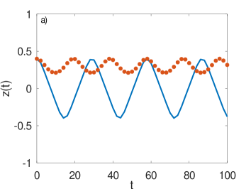
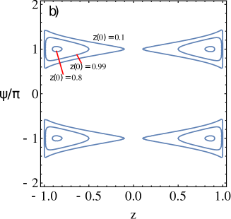
Figure 2: a) The dynamics of the relative imbalance $Z(t)$ for the LHY fluid ($\delta g=0$). Dot-line is for $\epsilon=1$ and the solid line is for $\epsilon=0.96$. Critical value $\epsilon_{c}=0.9872$. For both cases, oscillations are in the $\pi$-phase regime and the initial imbalance $Z(0)=0.4$. b) Phase portrait for the LHY fluid, where $\epsilon=1.96$.

In Fig. 2a the dynamics of the relative imbalance $Z$ for the LHY fluid ($\Lambda=0$)in $\pi$-phase mode is shown. From Eq.(30) we obtain $\epsilon_{c}=0.9872$. Here the dotted line is for the case $\epsilon=1$ and the solid line for $\epsilon=0.96$. One can see that can see that at $\epsilon>\epsilon_{c}$, the self-trapping regime appears.

In Fig. 2b the phase-portrait in ($Z,\psi$) plane for the LHY fluid case is presented. Is clearly seen the self-trapping of condensate in one of the wells under the action of quantum fluctuations. Note, that at these values of parameters, the self-trapping exists in the $\pi$-phase mode.

5 Numerical simulations

We also perform full numerical simulations of the modified GP equation with the double-well potential to the study the macroscopic quantum tunneling and self-trapping phenomena.

We start from the calculation of the ground state and exited state solutions with $N_{gr}=N_{ex}=1$ for given $\gamma$ and $\delta g$. Then using Eq. (8) we construct initial wave function for governing equation Eq. (5):

$$\Psi(x,t=0)=u(0)\Phi_{1}(x)+v(0)\Phi_{2}(x),$$ (31)

where $u(0)^{2}-v(0)^{2}=Z(t=0)$, By computing the full equation Eq. (5) we get the dependencies $Z(t),\phi(t)$.

For obtaining the relative imbalance $Z(t)$ and relative phase $\psi(t)$ one needs to calculate $N_{1,2}$ and $\phi_{1,2}$ as follows:

$$N_{1}(t)=\int_{-\infty}^{0}|\Psi(x,t)|^{2}dx,$$ (32)

$$N_{2}(t)=\int_{0}^{+\infty}|\Psi(x,t)|^{2}dx,$$ (33)

$$\phi_{1}(t)=\arctan{\frac{\int_{-\infty}^{0}\Im(\Psi(x,t))|\Psi(x,t)|^{2}dx}{\int_{-\infty}^{0}\Re(\Psi(x,t))|\Psi(x,t)|^{2}dx}},$$ (34)

$$\phi_{2}(t)=\arctan{\frac{\int_{0}^{+\infty}\Im(\Psi(x,t))|\Psi(x,t)|^{2}dx}{\int_{0}^{+\infty}\Re(\Psi(x,t))|\Psi(x,t)|^{2}dx}}$$ (35)

where $\Im$ and $\Re$ are the imaginary and real parts. For the following calculations the double-well potential parameters are $V_{0}=4,6,7$ with $l=1.5$.

In Fig. 3 the dependencies of the JO frequency $\omega_{J}$ : a) on $\gamma$ (the case of LHY-dimer at $\delta g=0$) and b) on $\delta g$ (the case when the LHY-term is neglected and $\delta g\neq 0$) are presented. There are two curves in this figure. The upper curve is for the frequency dependence of $Z(t)$ oscillations in the zero-phase regime, when $\psi=0$, and the lower one is for the case of $\pi$-phase regime $\psi=\pi$. One can see that at the very beginning of the two curves, they are described by equations Eq. (24) and Eq. (25) correspondingly. For both cases $Z(t=0)=0.02$.

As the LHY-term strength $\gamma$ increases, a localization phenomenon with $\langle Z\rangle\neq 0$ for $\gamma\approx 0.03$ occurs breaking the smooth behavior of the lower $\pi$-phase mode curve.

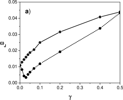
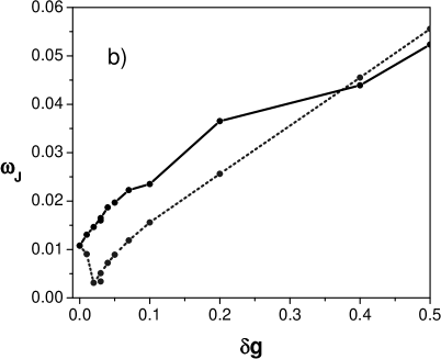
Figure 3: The frequency dependencies of the Josephson oscillations for a) the LHY-dimer, $\delta g=0$ (left graph) and b) the case when LHY-term is neglected. In both graphs upper solid lines are for zero-phase cases and lower dotted lines are for $\pi$-phase cases. In all cases the initial imbalance of Josephson oscillations $Z(t=0)=0.02$ for $V_{0}=7,\ l=1.5$.

The frequency dependencies for the same cases, but for larger intervals of $\gamma$ and $\delta g$ are presented in Fig. 4.

It should be noted that as seen in the left panel (the LHY fluid case) for $0<\gamma<1.5$ the mean value of the imbalance $\langle Z\rangle=0$, and $\langle Z\rangle\neq 0$ for $\gamma>1.6$. In the right panel (when the LHY term is neglected) for $0<\delta g<1.5$, the mean value of the imbalance $\langle Z\rangle=0$, and $\langle Z\rangle\neq 0$ for $\delta g>1.5$.

Figure 4: The frequency dependencies of the Josephson oscillations in the zero-phase mode: a) for different $LHY$-term $\gamma$ when $\delta g=0$; b) for different nonlinear term $\delta g$ when the LHY-term is neglected. Parameter $Z(t=0)=0.4$. Double-well potential parameters $V_{0}=6,\ l=1.5$ in both cases.

Figure 5: The time dependencies of $Z(t)$ for the LHY-fluid (with $\delta g=0$): a) $\gamma=0.02\$, b) $\gamma=0.025\$, c) $\gamma=0.03$. Solid lines are for the zero-phase and dot-lines are for the $\pi$-phase modes. The parameters of the trap potential are $V_{0}=7,\ l=1.5$. Everywhere initial imbalance $Z(t=0)=0.02$.

It is interesting to examine the evolution of the time dependencies of the population imbalance $Z(t)$ of the LHY-fluid near the symmetry breaking point that one can see at the beginning of the lower curve depicted in Fig. 3. In Fig. 5 the time dependencies of $Z(t)$ for three values of $\gamma$ are presented. One can see a transition of the $\pi$-phase mode into near the bifurcation point located between $\gamma=0.2$ and $\gamma=0.25$.

We consider Josephson oscillations of the atomic population imbalance $Z(t)$ ($\langle Z\rangle=0$) in the quasi-linear and self-localization regimes ($<Z>\neq 0$).

In Fig. 6, Josephson oscillations are presented based on the results obtained from the two-modes model and the numerical simulations. In all graphs, one can see phase shifts that increase with time.

In Fig.6a, the largest phase shift is observed when the nonlinear parameter $\delta g=1$ is large enough (at $\gamma=0$). For the LHY-fluid case, in Figs. 6b and 6c with the nonlinear parameters $\delta g=0$ and $\gamma=0.01$ (small enough), the phase shifts decrease. So, the accuracy of the two-modes method decreases at large times and large values of nonlinear parameters.

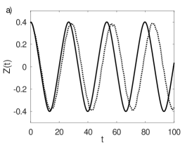
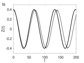
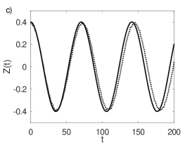
Figure 6: The time dependencies of the imbalance $Z(t)$ obtained from the two-mode model (solid lines) and the full numerical solution of Eq (5) (dot lines) for: a) $\delta g=1$, $\gamma=0$, (zero-phase); b) $\delta g=0$, $\gamma=0.01$, (zero-phase); c) $\delta g=0$, $\gamma=0.01$ ($\pi$-phase). Everywhere initial imbalance $Z(0)=0.4$. The parameters of the trap potential are $V_{0}=4,\ l=1.5$.

From Eq. (5) we see that if two nonlinear parameters are taken in opposite signs, they can suppress each other and the quasilinear (the Rabi) regime can be obtained. To create this regime we should calculate necessary values of the nonlinear parameters using Eq. (26). Thus we need also to calculate parameters $\alpha=\int_{-\infty}^{\infty}|\Phi_{1}(x)|^{4}dx$ and $\beta=\int_{-\infty}^{\infty}|\Phi_{1}(x)|^{5}dx$ that depend on values of the nonlinear parameters $\delta g$ and $\gamma$. In Figs. 7a and 7b, in order to observe effect of suppression, we choose the nonlinear parameters with opposite signs, $\delta g=-0.1,\ \gamma=0.1$ at the zero-phase and the $\pi$-phase modes. In Fig. 7c we choose corrected value for $\delta g$: $\delta g=-0.076,\ \gamma=0.1$ at the zero-phase mode. calculated from Eq.(26). One can see from Figs. 7a and 7b that there remain the phase shift between the solutions calculated based on the two-mode model and numerical simulations of the GP equation. Fig. 7c shows that the phase shifts of solutions obtained on the basis of the two-mode method and the numerical method have almost disappeared which indicates that the nonlinear effects have decreased and the mode of quasi-linear oscillations has been reached.

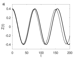
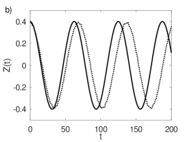
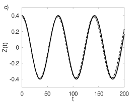
Figure 7: The time dependencies of the imbalance $Z(t)$ obtained from the two-modes model (solid lines) and the full numerical solution of Eq (5) (dot lines) for: a) $\delta g=-0.1$, $\gamma=0.1$ (zero-phase); b) $\delta g=-0.1$, $\gamma=0.1$ ($\pi$-phase), c) $\delta\ g=-0.076$, $\gamma=0.1$ (zero-phase) with initial imbalance $Z(0)=0.4$. The parameters of the trap potential are $V_{0}=4,\ l=1.5$.

To study the localization phenomenon, we consider the case of the LHY-fluid, when $\gamma\neq 0$ at $\delta g=0$. The results of calculation are given in Fig. 8 for three values of $\gamma=1.5;\ 1.6;\ 1.8$. As seen, the self-localization phenomenon is observed at $\gamma\simeq 1.6$. Two-mode model predict the existence of the ST transition, but the agreement with full numerical simulations of the MGP equation is only qualitative. This discrepancy is connected with neglect of nonlinear overlap integrals and thus to the error in the calculation of the tunneling amplitude $K$ [15].

Figure 8: The time dependencies of $Z(t)$ for the LHY-fluid case (with $\delta g=0$) when the LHY-term is a) $\gamma=1.5$; b) $\gamma=1.6$; c) $\gamma=1.8$. The parameters of the trap potential $V_{0}=6,\ l=1.5$.

In Figs. 9a, 9b and 9c the time dependencies of the imbalance $Z(t)$ at zero-phase and $\pi$-phase modes for $\gamma=0.5$, $\delta g=-0.1$ are presented for different values of the initial imbalance. As seen, an increase in the initial imbalance $Z(t=0)$ causes a change in the behavior of the dependencies $Z(t)$ and the emergence of the localization in both phase modes.

Figure 9: Time dependencies of $Z(t)$ for different initial imbalances: a) $Z(0)=0.4$; b) $Z(0)=0.6$; c) $Z(0)=0.6$. All graphs are presented for $\delta g=-0.1$, $\gamma=0.5$. Solid lines are for the $\pi$-phase $\psi(0)=\pi$ and dot lines are for the zero-phase $\psi(0)=0$ modes. Parameters of the trap potential $V_{0}=7,\ l_{0}=1.5$.

Let us estimate the parameters for the experiment with ²⁶Ka BEC, as performed in Ref. [13]. Transverse and longitudinal frequencies of the trap can be taken as, $\omega_{\perp}=2\pi\cdot 200$Hz, $\omega_{x}=2\pi\cdot 40$Hz and the number of atoms is $N=10^{3}\div 10^{4}$. Double-well potential can be generated by the superposition of the harmonic trap and periodic potential[17]. The barrier values for this double-well potential are $2\pi\cdot(160-240)$Hz when $V_{0}=4-6$. The atomic scattering length is about $a=50a_{0}$ and the scattering length between two components is about $\delta a=a_{0}$, where $a_{0}$ is the Bohr radius. The values of the scattering length can be varied using the Feshbach resonance technics. If we take $a=57.5a_{0}$, $\delta a=0$ and $N=10^{4}$, we get the values $\gamma=1.5$ and $\delta g=0$ and JO frequencies is $\omega_{J}=2\pi\cdot 2.8$Hz (Josephson oscillation around $\langle Z\rangle=0$). If we take $a=61.9a_{0}$, $\delta a=0$ and $N=10^{4}$, we get the values $\gamma=1.8$ and $\delta g=0$ and frequencies of atomic population imbalance $Z(t)$ is $\omega_{J}=2\pi\cdot 6$Hz(the frequency of self-localization mode) (see Fig.8). For the case $a=148a_{0}$, $\delta a=-0.25a_{0}$ and $N=10^{3}$, we get the values $\gamma=0.5$ and $\delta g=-0.1$ and thus frequencies of atomic population imbalance $Z(t)$ is $\omega_{J}=2\pi\cdot 1.35$Hz for zero-phase mode (Josephson oscillation around $\langle Z\rangle=0$) and $\omega_{J}=2\pi\cdot 3.6$Hz for $\pi$-phase mode(self-localization mode) (see Fig.9a).

6 Conclusion.

In conclusion, we have investigated the influence of quantum fluctuations on the dynamics of a two-component BEC in the double-well potential. In the scalar approximation and in a quasi-one-dimensional geometry, the problem is described by the modified GP equation with the additional LHY terms, corresponding to the beyond mean-field effects of quantum fluctuations.

We have derived a two-mode (dimer) model to describe the macroscopic quantum tunneling and self-trapping phenomena, when the quantum fluctuations are taken into account. The frequencies of the Josephson oscillations for zero- and $\pi$- phase modes are calculated. It is shown that the quasi-linear (i.e. the Rabi oscillations) regime of oscillations can be observed by a proper choice of the residual mean-field interactions between components of the BEC. It opens the possibility to measure the strength of quantum fluctuations.

The criterion for switching from the MQT regime to the ST one is obtained and applications for the observation of the LHY fluid have been discussed. Direct simulations of the modified GP equation with the Lee-Huang-Yang term, confirm predictions of the two-mode model for the JO frequencies. For the self-trapping regime, the agreement is only qualitative, due to limits of the two-mode model. Also, full simulations predict the self-trapping regime of the LHY fluid in the double-well potential.

In future will be interested to investigate the MQT and MST phenomena in the crossover regime from 3D and 2D geometry to one-dimensional geometry.

7 Acknowledgments

We thank B.Baizakov and E. N. Tsoy for fruitful discussions. The work was supported by the grant FA-F2-004 of Ministry of Innovative Development of the Republic of Uzbekistan.

References

- [1] Lee T D, Huang K, and Yang C N 1957 Phys. Rev. 106 1135.
- [2] Petrov D S 2015 Phys.Rev.Lett. 115 155302.
- [3] Petrov D S and Astrakharchik G E 2016 Rev. Lett. 117 100401.
- [4] Cabrera C R, Tanzi L, Sanz J, Naylor B, Thomas P, Cheiney P, and Tarruell L 2018 Science 359 301; Semeghini G, Ferioli G, Masi L, Mazzinghi C, Wolswijk L, Minardi F, Modugno M, Modugno G, Inguscio M, and Fattori M 2018 Phys. Rev. Lett. 120 235301; DÉrrico C, Burchianti A, Prevedelli M, Salasnich L, Ancilotto F, Modugno M, Minardi F, and Fort C 2019 Phys. Rev. research 1 033155
- [5] Ferrier-Barbut I, Kadau H, Schmitt M, Wenzel M, Pfau T 2016 Phys. Rev. Lett. 116 215301.
- [6] Rakshit D, Karpiuk T, Brewczyk M and Gajda M 2019 SciPost Phys. 6 079
- [7] Cappellaro A, Macr T, Bertacco G F, Salasnich L 2017 Scientific reports 7(1) 13358
- [8] Astrakharchik G E and Malomed B A, 2018 Phys. Rev. A 98 013631; Abdullaev F Kh, Gammal A, Kumar R K and Tomio L 2019 J. Phys. B: At. Mol. Opt. Phys. 52 195301; Otajonov Sh R, Tsoy E N, and Abdullaev F Kh 2019 Physics Letters A 383 125980.
- [9] Pathak M R, Nath A 2022 Scientific Reports 12 6904
- [10] Otajonov Sh R, Tsoy E N, and Abdullaev F Kh 2022 Phys. Rev. A 106 033309; Kartashov Y V, Lashkin M, Modugno M, and Torner L 2022 New J. Phys. 24 073012.
- [11] Jorgensen N B et al. 2018 Phys.Rev. Lett. 121 173403
- [12] Raghavan S, Smerzi A, Fantoni S, and Shenoy S R 1999 Phys. Rev. A 59 620
- [13] Skov T G et al. 2021 Phys.Rev.Lett. 126 230404
- [14] Pérez-García M V, Michinel H, Cirac J I, Lewenstein M, and Zoller P 1997 Phys. Rev. A 56 1424
- [15] Ananikian D and Bergeman T 2006 Phys. Rev. A 73 013604
- [16] Xiong B, Gong J, Han Pu, Bao W, and Li B 2009 Phys. Rev. A 79 013626
- [17] Albiez M, Gati R, Fölling J, Hunsmann S, Cristiani M, and Oberthaler M K 2005 Phys. Rev. Lett. 95 010402