A Graph-Based Approach to the Computation of Rate-Distortion and Capacity-Cost Functions with Side Information

Abstract

We consider the point-to-point lossy coding for computing and channel coding problems with two-sided information. We first unify these problems by considering a new generalized problem. Then we develop graph-based characterizations and derive interesting reductions through explicit graph operations, which reduce the number of decision variables. After that, we design alternating optimization algorithms for the unified problems, so that numerical computations for both the source and channel problems are covered. With the help of extra root-finding techniques, proper multiplier update strategies are developed. Thus our algorithms can compute the problems for a given distortion or cost constraint and the convergence can be proved. Also, extra heuristic deflation techniques are introduced which largely reduce the computational time. Numerical results show the accuracy and efficiency of our algorithms.

I Introduction

The point-to-point source and channel coding problems with side information and their duality were studied by many researchers [1, 2, 3]. The theoretical limits are described by the rate-distortion and the capacity-cost functions. These functions reflect the fundamental trade-offs between communication resources and other considerations. Important special cases include the Gelfand-Pinsker channel problem [4] and the Wyner-Ziv lossy compression problem [5].

As an extension of [5], some work [6] considered a lossy computing problem with decoder side information and obtained the rate-distortion function. However, the expression is in terms of an auxiliary random variable, for which however the intuitive meaning is not clear.

The notions of graph entropy and characteristic graph were introduced by Körner [7] and Witsenhausen [8] for zero-error coding problems. Orlitsky and Roche [9] extended the tools and obtained a graph-based characterization of the minimum rate for lossless computing with decoder side information. The auxiliary random variable involved therein is clearly represented by the independent set of a characteristic graph.

To better understand the lossy computing problem, a natural generalization of the graph entropy approach in [9] was given in  [10] and [11] by defining the $D$-characteristic graph, where an efficient but suboptimal coding scheme was obtained. In [12] and [13], Basu, Seo and Varshney generalized the independent sets to hyperedges and defined an $\epsilon$-characteristic hypergraph. The rate-distortion function was characterized for a limited class of distortion measure whose average represents the probability that the distance between $f$ and the reconstruction is larger than a given distortion level. Their generalization, however, cannot cope with general distortion measures.

The Blahut-Arimoto (BA) algorithm [14, 15] was the first attempt to numerically compute the classical channel capacity and rate-distortion function. It was also generalized to compute these limits in many other settings [16, 17, 18], including the source and channel coding problem with two-sided information in [19]. However, BA type algorithms cannot compute rate-distortion functions for any fixed distortion constraint, because it is the dual variables associated with the distortion constraints rather than the distortion constraints themselves that are fixed during iterations. Also, numerical computations for the lossy computing problem have not been considered.

Recently, some work [20, 21] introduced OT models and algorithms for numerical computation in information theory. Other work [22] designed algorithms based on Bregman Divergence. Their algorithms updated the dual variables during iterations, which guaranteed that the extra distortion constraints in the problems considered therein were satisfied.

In the current paper, we note the structural similarity of lossy computing and channel coding problems with two-sided information and introduce a new unified source-channel problem to analyze these problems together. By developing a bipartite-graph-based characterization for the new problem and performing feasible contractions on the graphs, we are able to largely reduce the number of edges and vertices and hence the number of decision variables for some important special cases. These efforts help with the computation of the trade-offs both analytically and numerically.

Applying the results to the lossy computing problem, we give the explicit meaning of the auxiliary random variable for any general distortion measures. Also, when two-sided information has a common part or the distortion is minimum, the characterization can be largely reduced. Our result naturally subsumes that in [12] as a special case by specifying a distortion measure. The capacity-cost function for channel with state information is analogously studied and reduced.

With the help of root-finding techniques, proper update strategies for the dual variables are added into an BA type alternating minimization process and algorithms are developed for the unified problem. The convergence of algorithms is proved. The specialized version of our algorithms can compute rate-distortion function for a given distortion constraint (or the capacity-cost function for a given cost constraint), overcoming the weaknesses of BA type algorithms. Also, an $O(\frac{1}{n})$ convergence for the optimal value can be showed for the lossy computing problem. Extra heuristic deflation techniques exploit the sparsity of solutions and greatly reduce computational cost for most cases. Numerical experiments show the accuracy and efficiency of our algorithms.

Compared with directly traversing the function with BA type algorithms in the expressions like in [19], our methods can greatly reduce computational complexity and compute the rate-distortion (capacity-cost) function for a given distortion (cost) constraint. Moreover, the graph characterizations combined with the heuristic deflation techniques can also accelerate the traditional BA type algorithms and hence the computation of the whole rate-distortion (capacity-cost) curves.

II Problem Formulation and Preliminaries

II-A The Lossy Computing Problem

Denote a discrete random variable by a capital letter and its finite alphabet by the corresponding calligraphic letter, e.g., $S_{1}\in\mathcal{S}_{1}$ and $\hat{Z}\in\hat{\mathcal{Z}}$. We use the superscript $n$ to denote an $n$-sequence, e.g., $S_{1}^{n}=(S_{1i})_{i=1}^{n}$.

Let $(S_{1i},S_{2i})\sim p(s_{1},s_{2}),i\in\{1,2,\cdots,n\}$ be i.i.d. random variables distributed over $\mathcal{S}_{1}\times\mathcal{S}_{2}$. Without loss of generality, assume $p(s_{1})>0$ and $p(s_{2})>0$, $\forall s_{1}\in\mathcal{S}_{1}$, $s_{2}\in\mathcal{S}_{2}$.

Consider the lossy computing problem with two-sided information depicted in Fig. 1. The source messages $S_{1}^{n}$ and $S_{2}^{n}$ are observed by the encoder and the decoder, respectively. Let $f:\mathcal{S}_{1}\times\mathcal{S}_{2}\to\mathcal{Z}$ be the function to be computed and $d:\mathcal{Z}\times\hat{\mathcal{Z}}\to[0,\infty)$ be a distortion measure. Denote $f(S_{1i},S_{2i})$ by $Z_{i}$ for $1\leq i\leq n$. Without ambiguity, we abuse the notation of $f$ and $g$ to denote their vector extensions, and define

$$f(s_{1}^{n},s_{2}^{n}) =\big{(}f(s_{1i},s_{2i})\big{)}_{i=1}^{n},$$

$$d(z^{n},\hat{z}^{n}) =\frac{1}{n}\sum_{i=1}^{n}d(z_{i},\hat{z}_{i}).$$

An $(n,2^{nR})$ code is defined by an encoding function

$$g_{e}:\mathcal{S}_{1}^{n}\to\{1,2,...,2^{nR}\}$$

and a decoding function

$$g_{d}:\{1,2,...,2^{nR}\}\times\mathcal{S}_{2}^{n}\to\hat{\mathcal{Z}}^{n}.$$

Then the decoded messages are $\hat{Z}^{n}=g_{d}(g_{e}(S_{1}^{n}),S_{2}^{n})$.

A rate-distortion pair $(R,D)$ is called achievable if there exists an $(n,2^{nR})$ code such that

$$\varlimsup_{n\to\infty}\mathbb{E}[d({Z}^{n},\hat{Z}^{n})]\leq D.$$

We define the rate-distortion function $R(D)$ to be the infimum of all the achievable rates such that $(R,D)$ is achievable.

Figure 1: Lossy computing with side information

II-B The Channel Coding Problem with State Information

Let $(\mathcal{X},p(y|x,s_{1},s_{2}),\mathcal{Y},\mathcal{S}_{1}\times\mathcal{S}_{2})$ be a discrete-memoryless channel with i.i.d. state information $(S_{1i},S_{2i})\sim p(s_{1},s_{2}),i\in\{1,2,\cdots,n\}$ distributed over $\mathcal{S}_{1}\times\mathcal{S}_{2}$. Also assume $p(s_{1})>0$, $\forall s_{1}\in\mathcal{S}_{1}$.

Consider the channel coding problem with two-sided state information depicted in Fig. 2. The encoder wishes to communicate a message $M$ which is uniformly distributed over $\{1,2,...,2^{nR}\}$ and independent of $(S_{1}^{n},S_{2}^{n})$ through a channel $(\mathcal{X},p(y|x,s_{1},s_{2}),\mathcal{Y},\mathcal{S}_{1}\times\mathcal{S}_{2})$. And states $S_{1}^{n}$ and $S_{2}^{n}$ are observed by the encoder and the decoder, respectively. Let $b:\mathcal{X}\times\mathcal{S}_{1}\times\mathcal{S}_{2}\to[0,\infty)$ be a cost measure depending on the input and the channel state. We abuse the notation of $b$ to denote its vector extension, and define

$$b(x^{n},s_{1}^{n},s_{2}^{n})=\frac{1}{n}\sum_{i=1}^{n}b(x_{i},s_{1i},s_{2i}).$$

An $(n,2^{nR})$ code is defined by an encoding function

$$g_{e}:\{1,2,...,2^{nR}\}\times\mathcal{S}_{1}^{n}\to\mathcal{X}^{n}$$

and a decoding function

$$g_{d}:\mathcal{Y}^{n}\times\mathcal{S}_{2}^{n}\to\{1,2,...,2^{nR}\}.$$

Then the channel inputs are $X^{n}=g_{e}(M,S_{1}^{n})$ and the decoded messages are $\hat{M}=g_{d}(Y^{n},S_{2}^{n})$.

A capacity-cost pair $(R,B)$ is called achievable if there exists an $(n,2^{nR})$ code such that

$$\mathbb{P}[\hat{M}\neq M]\to 0,n\to\infty,$$

and

$$\varlimsup_{n\to\infty}\mathbb{E}[b(X^{n},S_{1}^{n},S_{2}^{n})]\leq B.$$

We define the rate-distortion function $C(B)$ to be the supremum of all the achievable rates such that $(R,B)$ is achievable.

Figure 2: Channel coding with state information

II-C Preliminary Results

We can adapt the results of [1] and formulate the expressions for these two trade-offs.

Lemma 1.

The rate-distortion function for lossy computing and the capacity-cost function with two-sided information are given by

$$R(D)=\min_{\begin{subarray}{c}p(u|s_{1}):\ \exists g,\\ \mathbb{E}[d(f(S_{1},S_{2}),g(U,S_{2}))]\leq D\end{subarray}}I(U;S_{1})-I(U;S_{2}),$$ (1)

$$C(B)=\max_{\begin{subarray}{c}p(u|s_{1}):\ \exists g,\\ \mathbb{E}[b(g(U,S_{1}),S_{1},S_{2})]\leq B\end{subarray}}I(U;Y,S_{2})-I(U;S_{1}).$$ (2)

The proof is in the same manner as in [1]. The coding scheme is similar to the lossy compression case $f(s_{1},s_{2})=s_{1}$ and channels without input cost discussed in [1]. Only the objectives for coding are different and the additional constraints need to be modified.

II-D Bipartite Graph

Let $\mathscr{G}=(\mathscr{V},\mathscr{E})$ be a simple graph with the vertex set $\mathscr{V}$ and edge set $\mathscr{E}$. It is a bipartite graph [23] if $\mathscr{V}$ can be split into the disjoint sets $\mathscr{V}_{1}$ and $\mathscr{V}_{2}$ so that each edge in $\mathscr{E}$ has one end in $\mathscr{V}_{1}$ and one end in $\mathscr{V}_{2}$. Denote by $\mathscr{G}[\mathscr{V}_{1},\mathscr{V}_{2}]$ such a bipartite graph. A bipartite graph $\mathscr{G}[\mathscr{V}_{1},\mathscr{V}_{2}]$ is called complete if every vertex in $\mathscr{V}_{1}$ is joined to every vertex in $\mathscr{V}_{2}$.

Let $\mathscr{G}[\mathscr{V}_{1},\mathscr{V}_{2}]$ be a bipartite graph with the edge set $\mathscr{E}$. If there is a weight function $\omega:\mathscr{E}\to\mathbb{R}$, then the graph $\mathscr{G}[\mathscr{V}_{1},\mathscr{V}_{2}]$ associated with the weight $\omega$ is called a weighted bipartite graph, denoted by $(\mathscr{G}[\mathscr{V}_{1},\mathscr{V}_{2}],\omega)$. In this work, we only consider weighted bipartite graphs with weight functions $\omega(e)\in[0,1]$, $\forall e\in\mathscr{E}$.

III The Unified Source-Channel Problem

The similarity between (1) and (2) is often called the source-channel duality. Still, more can be revealed by breaking such a border lying between source and channel problems and examining their substantial structures as optimization problems. Both problems are convex and the convexity mainly arises from the mutual information term $I(U;S_{1})$ directly depending on the decision variable $p(u|s_{1})$. Also, the distortion or cost constraints are both linear. These observations motivate us to generalize them to a new source-channel problem, so that both problems can be studied together.

We are going to show (1), (2) and their interesting reductions are all special cases of the new problem (3). Therefore, designing algorithms for (3) is enough to solve both (1) and (2).

Let $\mathscr{E}\subseteq\mathcal{V}\times\mathcal{U}$ and for each $v\in\mathcal{V}$, there exists some $u\in\mathcal{U}$ such that $(v,u)\in\mathscr{E}$. We consider the following optimization problem with a given loss function $l:\mathscr{E}\times\mathcal{W}\to[0,\infty)$,

$$\min_{p(u|v)} I(U;V)-I(U;W),$$ (3a)

$$\mathrm{s.t.} \mathbb{P}[(V,U)\in\mathscr{E}]=1,$$ (3b)

$$\mathbb{E}[l(V,U,W)]\leq L,$$ (3c)

where the distribution of $V$ and the conditional distribution $W|e$ for $e\in\mathscr{E}$ are also given. In other words, we always have

$$p(u,v,w)=p(v)p(u|v)p(w|u,v),$$

where $p(u|v)$ is the decision variable, while $p(v)$ and $p(w|u,v)$ are given (the latter is defined as $0$ when $(v,u)\notin\mathscr{E}$).

Without loss of generality, we assume that for any $v$,

$$p(v)>0.$$ (4)

Also, for any $w$,

$$\exists(v,u)\in\mathscr{E},\ \mathrm{s.t.}\ p(w|u,v)>0.$$ (5)

Or we can just eliminate $v$ and $w$ that do not satisfy the assumptions.

Define the target-loss function to be the optimal value of the problem (3), which is denoted by $T(L)$.

In the remaining part of this section, the problem is transformed into an equivalent form in Section III-A and its properties for different loss constraints $L$ are investigated in Section III-B, preparing for the designing of algorithms.

III-A Properties and Equivalent Forms of the Problem

It is easy to see that the problem (3) only depends on the loss function $l$ through

$$\tilde{l}(v,u)\triangleq\sum_{w^{\prime}}p(w^{\prime}|u,v)l(v,u,w^{\prime}).$$ (6)

We denote by $\mathrm{supp}(\bm{p})\triangleq\{(v,u)|p(u|v)>0\}$ the support of $p(u|v)$ as a function of $(v,u)$, then (3b) is equivalent to $\mathrm{supp}(\bm{p})\subseteq\mathscr{E}$.

The problem (3) is equivalent to the following

$$\min_{p(u|v)} \sum_{(v,u)\in\mathscr{E},w}p(v)p(u|v)p(w|u,v)\log\frac{p(u|v)}{p(u|w)},$$ (7a)

$$\mathrm{s.t.}\ \mathrm{supp}(\bm{p})\subseteq\mathscr{E},$$ (7b)

$$\sum_{(v,u)\in\mathscr{E}}p(v)p(u|v)\tilde{l}(v,u)\leq L,$$ (7c)

where

$$p(u|w)=\frac{p(u,w)}{p(w)}=\frac{\sum_{v:(v,u)\in\mathscr{E}}p(v)p(u|v)p(w|u,v)}{\sum_{(v,u)\in\mathscr{E}}p(v)p(u|v)p(w|u,v)}.$$ (8)

is the conditional distribution of $U$ given $W$, which is defined when $p(w)=\sum_{(v,u)\in\mathscr{E}}p(v)p(u|v)p(w|u,v)>0$.

To simplify the notation, we rewrite the conditional distribution of $U|V$ and $U|W$ by $\bm{q}$ and $\bm{r}$, respectively. Define

$$Loss(\bm{q})=\sum_{(v,u)\in\mathscr{E}}p(v)q(u|v)\tilde{l}(v,u).$$ (9)

and the generalized Kullback-Leibler (K-L) divergence

$$GD_{\mathscr{E}}(\bm{q}||\bm{r})=\sum_{(v,u)\in\mathscr{E},w}p(v)q(u|v)p(w|u,v)\log\frac{q(u|v)}{r(u|w)}.$$ (10)

The generalized K-L divergence is not necessarily nonnegative as the classical one, which is defined between two distributions on the same set. But it is nonnegative if $\bm{q}$ and $\bm{r}$ are two conditional distributions on the same set.

With this definition, the objective function of (3) can be written as $\mathcal{O}(\bm{p})=GD_{\mathscr{E}}(\bm{p}||\bm{p})$. The following theorem shows $\bm{p}$ on the second position can be relaxed and this gives an equivalent form of the problem. It motivates our alternating minimization algorithms.

It can be seen from (8) that for any feasible solution $\bm{p}$ of (7), $\mathrm{supp}(p(u|w))\subseteq\mathscr{F}$ as a function of $(u,w)$, where

$$\mathscr{F}=\left\{(u,w)|\exists v,(v,u)\in\mathscr{E},p(w|u,v)>0\right\}.$$ (11)

Then the following equivalent form of (3) is immediate, which is a variant of BA type equivalent form.

Lemma 2.

The problem (3) has the same optimal value $T(L)$ with the following problem.

$$\min_{\bm{q},\bm{r}}\ GD_{\mathscr{E}}(\bm{q}||\bm{r}),$$ (12a)

$$\mathrm{s.t.}\ \mathrm{supp}(\bm{q})\subseteq\mathscr{E},$$ (12b)

$$Loss(\bm{q})\leq L,$$ (12c)

$$\mathrm{supp}(\bm{r})\subseteq\mathscr{F}.$$ (12d)

The proof of the theorem can be found in Appendix D. The equivalent problem (12) and the original one (3) share good properties, which help with their solution.

Lemma 3.

Both (12) and (3) are convex optimization problems.

The proof can also be found in Appendix A.

III-B Properties of the Problem for Different Loss Constraints

The newly defined target-loss function preserves the key properties of the original rate-distortion and capacity-cost functions, as is summarized as follows and proved in Appendix A.

Lemma 4.

The target-loss function $T(L)$ is decreasing and convex in $L\in[0,\infty)$.

Further investigation into the problem enables us to identify trivial cases and focus on difficulties we really need to tackle. We first define the boundaries for different cases of problems (3) to be

$$L_{min}\triangleq\min_{\mathrm{supp}(\bm{q})\subseteq\mathscr{E}}\left\{Loss(\bm{q})\right\},$$ (13)

$$L_{max}\triangleq\min\left\{L\geq 0\bigg{|}T(L)=\min_{L^{\prime}\geq 0}T(L^{\prime})\right\},$$ (14)

$$L_{Max}\triangleq\max_{\mathrm{supp}(\bm{q})\subseteq\mathscr{E}}\left\{Loss(\bm{q})\right\}.$$ (15)

Then it is easy to find that $L_{min}\leq L_{max}\leq L_{Max}$. Also, $L_{min}$ and $L_{max}$ are easy to compute by the following formula,

$$L_{min}=\sum_{v}p(v)\min_{u:(v,u)\in\mathscr{E}}\left\{\tilde{l}(v,u)\right\},$$ (16)

$$L_{Max}=\sum_{v}p(v)\max_{u:(v,u)\in\mathscr{E}}\left\{\tilde{l}(v,u)\right\}.$$ (17)

In contrast, $L_{max}$ does not have an explicit formula in general, except for special cases such as in the lossy computing problem discussed in Section V.

The problem (3) can be classified into the following cases with different ranges of $L$, which directly help with the computation.

Theorem 1.

For the problem (3), we have the following.

1. For $0\leq L<L_{min}$, (3) is infeasible, so $T(L)=\infty$.

2. For $L\geq L_{min}$, (3) is feasible and $T(L_{min})<\infty$.

3. For $L>L_{min}$, the Slater Constraint Qualification (SLCQ) is satisfied, the Karush-Kuhn-Tucker (KKT) conditions are both necessary and sufficient for optimality.

4. $T(L)$ is continuous in $L\in[L_{min},\infty)$.

5. $T(L)$ is strictly decreasing in $L\in[L_{min},L_{max}]$. In this case, the optimal value of the problem (3) is achieved as equality holds in the loss constraint.

6. For $L\geq L_{Max}$, the loss constraint (3c) is always satisfied and can be neglected.

Theorem 1 can be easily derived from Lemma 4 and the proof is omitted. Also note that the problem (12) shares the same properties described in Theorem 1.

For the problem (3), we can first compute $D_{min}$ and $D_{Max}$ by (16)(17) and compare $D$ with them. By Theorem 1, we only need to compute the target-loss function for $D\geq D_{min}$. The ideas are briefly summarized here and details will be described in Section VII.

1. For $L=L_{min}$, the problem can be solved by a variant BA type algorithm.

2. For $L\in(L_{min},L_{Max})$, the problem is solved by our improved alternating minimization algorithm.

3. For $L\geq L_{Max}$, after directly eliding the constraint (3c), the problem can be solved by a variant BA type algorithm.

IV Graph-Based Characterizations

We introduce graph-based characterizations for the problem (3) and explore its reductions, which helps with its solution both analytically and numerically.

IV-A Construction and Operations on the Graph Characterization

In the problem (3), the decision variable $p(u|v)$ is a transition probability from $\mathcal{V}$ to $\mathcal{U}$. This observation motivates us to represent $v\in\mathcal{V}$ and $u\in\mathcal{U}$ by vertices, connect $v$ and $u$ when $(v,u)\in\mathscr{E}$ and view each $p(u|v)$ as the weight on the edge. This constructs a bipartite graph $G[\mathcal{V},\mathcal{U}]$ with edge set $\mathscr{E}$. Denote by $\mathscr{E}^{u}\subseteq\mathcal{V}$ and $\mathscr{E}_{v}\subseteq\mathcal{U}$ the set of vertices adjacent to $u$ and $v$, respectively.

We say $\omega$ is a feasible weight on a bipartite graph $G[\mathcal{V},\mathcal{U}]$ with edge set $\mathscr{E}$ if

1. for any $v\in\mathcal{V}$,

   $$\sum_{u\in\mathscr{E}_{v}}\omega(v,u)=1,$$

2. $\omega$ satisfies the loss constraint

   $$\sum_{(v,u)\in\mathscr{E}}p(v)\omega(v,u)\tilde{l}(v,u)\leq L.$$

In this case, we denote the bipartite graph with a feasible weight by $(G[\mathcal{V},\mathcal{U}],\omega)$.

Definition 1.

The characteristic bipartite graph for (3) is defined as a bipartite graph $G_{\chi}[\mathcal{V},\mathcal{U}]$ with edge set $\mathscr{E}$.

Each feasible solution $\bm{p}$ of (3) naturally corresponds to a feasible weight $\omega_{\bm{p}}$ on $G_{\chi}[\mathcal{V},\mathcal{U}]$ with $\omega_{\bm{p}}(v,u)=p(u|v)$. The problem (3) is then an optimization problem over all $\omega_{\bm{p}}(v,u)$. Or equivalently, we have a canonical graph characterization immediately.

Lemma 5.

Let $T(L)$ be the target-loss function, then

$$T(L)= \min_{(G_{\chi}[\mathcal{V},\mathcal{U}],\omega_{\bm{p}})}\mathcal{O}(\bm{p}),$$ (18)

where the minimum is taken over all feasible weights $\omega_{\bm{p}}$ on $G_{\chi}[\mathcal{V},\mathcal{U}]$.

We introduce a contraction operation for a bipartite graph $(G[\mathcal{V},\mathcal{U}],\omega_{\bm{p}})$, which will be proved to decrease the objective function and keep the weight feasible.

Definition 2.

Let $G[\mathcal{V},\mathcal{U}]$ be a bipartite graph with edge set $\mathscr{E}$ and $G^{\prime}[\mathcal{V},\mathcal{U}^{\prime}]$ is its subgraph with edge set $\mathscr{E}^{\prime}$ ( $\mathcal{U}^{\prime}\subseteq\mathcal{U}$ and $\mathscr{E}^{\prime}\subseteq\mathscr{E}$). We say a feasible contraction transforms $(G[\mathcal{V},\mathcal{U}],\omega_{\bm{p}})$ into $(G^{\prime}[\mathcal{V},\mathcal{U}^{\prime}],\omega_{\bm{p}^{\prime}})$ if

1. there exists a function $h:\mathcal{U}\to\mathcal{U}^{\prime}$ such that for any $(v,u)\in\mathscr{E}$, $(v,h(u))\in\mathscr{E}^{\prime}$;

2. for any $(v,u)\in\mathscr{E}$,

   $$\tilde{l}(v,h(u))\leq\tilde{l}(v,u);$$ (19)

3. for any $(v,u)\in\mathscr{E}$ and $w\in\mathcal{W}$,

   $$p(w|h(u),v)=p(w|u,v);$$ (20)

4. $\bm{p}^{\prime}$ is naturally induced by $h$ from $\bm{p}$, to be precise, for any $(v,u^{\prime})\in\mathscr{E}^{\prime}$,

   $$\omega_{\bm{p}^{\prime}}(v,u^{\prime})\triangleq p^{\prime}(u^{\prime}|v)=\sum_{\begin{subarray}{c}u\in\mathscr{E}_{v}\\ h(u)=u^{\prime}\end{subarray}}p(u|v).$$ (21)

Remark 1.

To show the definition is well-defined, we need to show $\bm{p}^{\prime}$ induced by $h$ from $\bm{p}$ is actually a feasible weight on $G^{\prime}[\mathcal{V},\mathcal{U}]$. The well-definedness of Definition 2 as well as Definition 3 can be found in the proof of Lemma 6.

Theorem 2.

If there exists a subgraph $G^{\prime}[\mathcal{V},\mathcal{U}^{\prime}]$ of $G_{\chi}[\mathcal{V},\mathcal{U}]$. such that each feasible weight $\omega_{\bm{p}}$ on $G_{\chi}[\mathcal{V},\mathcal{U}]$ can be transformed into some feasible weight $\omega_{\bm{p}^{\prime}}$ on $G^{\prime}[\mathcal{V},\mathcal{U}^{\prime}]$ by a feasible contraction. Then

$$T(L)= \min_{(G^{\prime}[\mathcal{V},\mathcal{U}^{\prime}],\omega_{\bm{p}})}\mathcal{O}(\bm{p}).$$ (22)

Note that $G^{\prime}[\mathcal{V},\mathcal{U}^{\prime}]$ always has less vertices and edges than $G_{\chi}[\mathcal{V},\mathcal{U}]$. So the number of decision variables is reduced.

Theorem 2 serves as a basic tool for the reduction of the problem in various special cases, and it will be proved along with its generalized form Theorem 3. In these cases, the feasible contraction is always chosen to be uniform in $\omega_{\bm{p}}$, that is, there exists one feasible contraction which transforms any $\omega_{\bm{p}}$ into some $\omega_{\bm{p}^{\prime}}$ and makes the latter satisfy the condition.

Two special cases are discussed in Section IV-B and IV-C. We will apply and extend these results to our main objects in Section V and VI.

IV-B When Two-Sided Information Has a Common Part

To further simplify the graph characterization in the case when two-sided information has a common part, we generalizes the ideas of the Gács-Körner-Witsenhausen common information. We find the contraction function $h$ can be allowed to be dependent on the common part.

Definition 3.

Let $G[\mathcal{V},\mathcal{U}]$ be a bipartite graph with edge set $\mathscr{E}$ and $G^{\prime}[\mathcal{V},\mathcal{U}^{\prime}]$ is its subgraph with edge set $\mathscr{E}^{\prime}$ ( $\mathcal{U}^{\prime}\subseteq\mathcal{U}$ and $\mathscr{E}^{\prime}\subseteq\mathscr{E}$). We say a generalized feasible contraction transforms $(G[\mathcal{V},\mathcal{U}],\omega_{\bm{p}})$ into $(G^{\prime}[\mathcal{V},\mathcal{U}^{\prime}],\omega_{\bm{p}^{\prime}})$ if

1. $\mathcal{V}=\cup_{k=1}^{K}\mathcal{V}_{k}$ and $\mathcal{W}=\cup_{k=1}^{K}\mathcal{W}_{k}$ be partitions satisfying the strict separation condition: for any $(v,w)$,

   $$\exists u,\ p(w|u,v)>0\Rightarrow\exists k,\ v\in\mathcal{V}_{k},\ w\in\mathcal{W}_{k};$$ (23)

2. there exist functions $h_{k}:\mathcal{U}\to\mathcal{U}^{\prime}$, $k=1,2,...,K$ such that for any $(v,u)\in\mathscr{E}$, $(v,h_{k}(u))\in\mathscr{E}^{\prime}$;

3. for any $v\in\mathcal{V}_{k}$ and $(v,u)\in\mathscr{E}$,

   $$\tilde{l}(v,h_{k}(u))\leq\tilde{l}(v,u);$$ (24)

4. for any $v\in\mathcal{V}_{k}$, $(v,u)\in\mathscr{E}$ and $w\in\mathcal{W}_{k}$,

   $$p(w|h_{k}(u),v)=p(w|u,v);$$ (25)

5. for any $v\in\mathcal{V}_{k}$ and $(v,u^{\prime})\in\mathscr{E}^{\prime}$,

   $$\omega_{\bm{p}^{\prime}}(v,u^{\prime})\triangleq p^{\prime}(u^{\prime}|v)=\sum_{\begin{subarray}{c}u\in\mathscr{E}_{v}\\ h_{k}(u)=u^{\prime}\end{subarray}}p(u|v).$$ (26)

The aim of introducing the generalized feasible contraction is to simplify the graph without increasing the value of the objective function, which is shown by the following result.

Lemma 6.

Suppose a generalized feasible contraction transforms $(G[\mathcal{V},\mathcal{U}],\omega_{\bm{p}})$ into $(G^{\prime}[\mathcal{V},\mathcal{U}],\omega_{\bm{p}^{\prime}})$. Then $\omega_{\bm{p}^{\prime}}$ is actually a feasible weight and attains less value of the objective function.

The proof can be found in Appendix C.

Theorem 3.

If there exists a subgraph $G^{\prime}[\mathcal{V},\mathcal{U}^{\prime}]$ of $G_{\chi}[\mathcal{V},\mathcal{U}]$, such that each feasible weight $\omega_{\bm{p}}$ on $G_{\chi}[\mathcal{V},\mathcal{U}]$ can be transformed into some feasible weight $\omega_{\bm{p}^{\prime}}$ on $G^{\prime}[\mathcal{V},\mathcal{U}^{\prime}]$ by a generalized feasible contraction. Then

$$T(L)= \min_{(G^{\prime}[\mathcal{V},\mathcal{U}^{\prime}],\omega_{\bm{p}})}\mathcal{O}(\bm{p}).$$ (27)

Proof:

Note that the edge set of $G^{\prime}[\mathcal{V},\mathcal{U}^{\prime}]$ is contained in which of $G_{\chi}[\mathcal{V},\mathcal{U}]$, and hence any feasible weight on $G^{\prime}[\mathcal{V},\mathcal{U}^{\prime}]$ must be a feasible weight on $G_{\chi}[\mathcal{V},\mathcal{U}]$ by zero extension. This gives one direction. The other is immediate from Lemma 6. ∎

Now we formally investigate an important case when two-sided information has a common part, which will be used in Section V and VI. Suppose $W=(\tilde{W},V^{\prime})$ and $p(\tilde{w},v^{\prime}|u,v)=p(\tilde{w}|u,v)p(v^{\prime}|v)$. We will see the meaning of $V^{\prime}$ will be the decoder side information, whose distribution is given and may be correlated to the encoder side information $V$.

By relabeling the alphabet $\mathcal{V}$ and $\mathcal{V^{\prime}}$, we can arrange $p(v,v^{\prime})$ in a block diagonal form with the maximum positive number $K$ of nonzero blocks. The common part [25] of $V$ and $V^{\prime}$ is the random variable $V_{0}$ that takes value $k$ if $(V,V^{\prime})$ is in block $k$, $k=1,...,K$. In this case, there exists some function $g_{1}:\mathcal{V}\to\{1,...,K\}$, $g_{2}:\mathcal{V}^{\prime}\to\{1,...,K\}$ such that $V_{0}=g_{1}(V)=g_{2}(V^{\prime})$.

Let $\mathcal{V}_{k}=g_{1}^{-1}(k)$ and $\mathcal{W}_{k}=\tilde{\mathcal{W}}\times g_{2}^{-1}(k)$, $k=1,...,K$. Then for any $v\in\mathcal{V}_{k}$, $w=(\tilde{w},v^{\prime})\in\mathcal{W}_{k^{\prime}}$, we always have $p(v,v^{\prime})=0$ if $k\neq k^{\prime}$, and hence $p(w|u,v)=0$ for any $u$. So the strict separation condition is satisfied in this case. Also, the family of functions $h_{k}$ is dependent on the value of the common information.

IV-C The Minimum Loss Case

Consider the problem (18) when $L=L_{min}$. In this case, $\omega_{\bm{p}}(v,u)=p(u|v)>0$ only if the following condition is satisfied,

$$\tilde{l}(v,u)=\min_{u^{\prime}\in\mathscr{E}_{v}}\left\{\tilde{l}(v,u^{\prime})\right\}.$$ (28)

We can construct a subgraph $G_{*}[\mathcal{V},\mathcal{U}]$ of $G_{\chi}[\mathcal{V},\mathcal{U}]$ by defining its edge set $\mathscr{E}_{*}$. Let $e=(v,u)$ be an edge if (28) is satisfied by $v\in\mathcal{V}$ and $u\in\mathscr{E}_{v}$.

It is immediate from (28) that for each $v\in\mathcal{V}$, there is at least one $u\in\mathcal{U}$ such that $(v,u)\in\mathscr{E}_{*}$. Also, $\mathscr{E}_{*v}\subseteq\mathscr{E}_{v}$ and $\mathscr{E}_{*}^{u}\subseteq\mathscr{E}^{u}$.

By the construction, the information about the loss constraint has been absorbed into the structure of the graph $G_{*}[\mathcal{V},\mathcal{U}]$. Let $h(u)=u$ in the feasible contraction and we can apply Theorem 2 to reduce the graph. Also, for the resulting graph the second condition (the loss constraint) of feasible weights is redundant and hence we have

Theorem 4.

For the minimum loss case,

$$T(L_{min})= \min_{(G_{*}[\mathcal{V},\mathcal{U}],\omega_{\bm{p}})}\mathcal{O}(\bm{p}),$$ (29)

and equivalently, the minimum can be taken over all weights $\omega_{\bm{p}}$ on $G_{*}[\mathcal{V},\mathcal{U}]$ induced by some $\bm{p}$.

Remark 2.

By simply deleting vertices in $\mathcal{U}$ not adjacent to any edges, we can construct the subgraph $G_{*}[\mathcal{V},\mathcal{U}^{\prime}]$, where $\mathcal{U}^{\prime}\subseteq\mathcal{U}$. Then Theorem 4 is also true if $G_{*}[\mathcal{V},\mathcal{U}]$ is replaced by $G_{*}[\mathcal{V},\mathcal{U}^{\prime}]$.

V Lossy Computing Problems with Side Information

V-A Canonical Graph Characterization

We first show this problem can be reduced to special cases of (3) and the canonical graph characterization for this problem can be derived as well. Some interesting reductions will be discussed subsequently.

By Lemma 1,

$$R(D)=\min_{\begin{subarray}{c}p(u|s_{1}):\ \exists g,\\ \mathbb{E}[d(f(S_{1},S_{2}),g(U,S_{2}))]\leq D\end{subarray}}I(U;S_{1})-I(U;S_{2}).$$ (30)

We interpret the right hand side in a graph-based manner. Let $\mathcal{V}=\mathcal{S}_{1}$ and $\mathcal{W}=\mathcal{S}_{2}$, where $p(s_{2}|u,s_{1})=p(s_{2}|s_{1})$ is given. Also, let $l(s_{1},u,s_{2})=d(f(s_{1},s_{2}),g(u,s_{2}))$. Then for each feasible solution $(g,p(u|s_{1}))$, We can construct a complete bipartite graph $G_{g}[\mathcal{V},\mathcal{U}]$ and $\omega_{\bm{p}}(v,u)=p(u|v)$ is a feasible weight on the graph. So we have

$$R(D)=\min_{g,(G_{g}[\mathcal{V},\mathcal{U}],\omega_{\bm{p}})}\mathcal{O}(\bm{p}).$$

We can always assume that for any $u_{1},u_{2}\in\mathcal{U}$, there exists some $s_{2}$ such that $g(u_{1},s_{2})\neq g(u_{2},s_{2})$. Otherwise, we apply a feasible contraction on $(G_{g}[\mathcal{V},\mathcal{U}],\omega_{\bm{p}})$ as follows. First classify $u$ by the value of $g(u,s_{2})$, that is, $u_{1}$ and $u_{2}$ are classified into one equivalent class if $g(u_{1},s_{2})=g(u_{2},s_{2})$ for each $s_{2}\in\mathcal{S}_{2}$. This leads to a partition $\mathcal{U}=\cup_{i}\mathcal{U}_{i}$. Then choose one representative $u_{i}$ from each class $U_{i}$. Finally, let $h(u)=u_{i}$ if $u\in u_{i}$. Then (20) and (19) can be easily verified. Denote the graph after contraction by $(G_{1}[\mathcal{V},\cup_{i}\{u_{i}\}],\omega_{\bm{p}^{\prime}})$. By Lemma 6, $\omega_{\bm{p}^{\prime}}$ is a feasible weight on $G_{1}[\mathcal{V},\cup_{i}\{u_{i}\}]$ and $\mathcal{O}(\bm{p}^{\prime})\leq\mathcal{O}(\bm{p})$. But $G_{1}[\mathcal{V},\cup_{i}\{u_{i}\}]$ satisfies the condition we assume.

Let $\mathcal{U}^{\prime}=\mathcal{Z}^{\mathcal{S}_{2}}$ and construct a complete bipartite graph $G[\mathcal{V},\mathcal{U}^{\prime}]$. We can observe that any $G_{g}[\mathcal{V},U]$ can be seen as a subgraph of $G[\mathcal{V},\mathcal{U}^{\prime}]$ by an injection taking $u$ to $(g(u,s_{2}))_{s_{2}\in\mathcal{S}_{2}}$, as well as edges adjacent to these vertices. Hence each feasible weight $\omega_{\bm{p}}$ on $G_{g}[\mathcal{V},U]$ can be seen as a feasible weight on $G[\mathcal{V},\mathcal{U}^{\prime}]$ after zero extension. So we have

$$\min_{(G[\mathcal{V},\mathcal{U}^{\prime}],\omega_{\bm{p}})}\mathcal{O}(\bm{p})\leq\min_{g,(G_{g}[\mathcal{V},\mathcal{U}],\omega_{\bm{p}})}\mathcal{O}(\bm{p}).$$

Finally, we define $g(u,s_{2})=\hat{z}_{s_{2}}$ for each $u^{\prime}=(\hat{z}_{s_{2}})_{s_{2}\in\mathcal{S}_{2}}$ and $s_{2}\in\mathcal{S}_{2}$. Then $g,(G[\mathcal{V},\mathcal{U}^{\prime}],\omega_{\bm{p}})$ is a feasible solution of the left hand side. So we have

$$R(D)=\min_{g,(G_{g}[\mathcal{V},\mathcal{U}],\omega_{\bm{p}})}\mathcal{O}(\bm{p})=\min_{(G[\mathcal{V},\mathcal{U}^{\prime}],\omega_{\bm{p}^{\prime}})}\mathcal{O}(\bm{p}^{\prime}).$$

We also call this result the canonical graph characterization for the problem (1). Or equivalently, the above graph-based derivative leads to the following result.

Lemma 7.

We have the following characterization for the lossy computing problem,

$$R(D)=\min_{\begin{subarray}{c}p(u|s_{1}):U=(\hat{Z}_{s_{2}})_{s_{2}\in\mathcal{S}_{2}}\\ \mathbb{E}[d(f(S_{1},S_{2}),\hat{Z}_{S_{2}})]\leq D\end{subarray}}I(U;S_{1})-I(U;S_{2}).$$ (31)

The right hand side is a special case of (3). Let $U=(\hat{Z}_{s_{2}})_{s_{2}\in\mathcal{S}_{2}}$, $V=S_{1}$ and $W=S_{2}$, where $p(s_{2}|u,s_{1})=p(s_{2}|s_{1})$ is given. Also, let $l(s_{1},u,s_{2})=d(f(s_{1},s_{2}),\hat{z}_{s_{2}})$ where $u=(\hat{z}_{s_{2}})_{s_{2}\in\mathcal{S}_{2}}$. So the canonical graph characterization for (3) and (1) actually coincide.

In this specific case, since $p(w|u,v)=p(s_{2}|s_{1})=p(w|v)$, $U-V-W$ is a Markov chain. And hence we have

$$I(U;V)-I(U;W)=I(U;V|W)\geq 0.$$ (32)

So the optimal value is always nonnegative.

Also, the explicit value of $L_{max}$ can be computed, which is useful for the computation. The proof is given in Appendix B.

Proposition 1.

For the rate-distortion problem,

$$L_{max}=\min_{u\in\mathcal{U}}\left\{\sum_{v}p(v)\tilde{l}(v,u)\right\}.$$ (33)

For $L\geq L_{max}$, the optimal value is $0$ and can be obtained by some $q(u|x)=\mathds{1}{(u=u_{0})}$.

V-B When Two-Sided Information Has a Common Part

Let $S_{0}\in\{1,...,K\}$ be the common part of $S_{1}$ and $S_{2}$ and $S_{0}=g_{1}(S_{1})=g_{2}(S_{2})$. We start from the canonical graph characterization of this problem and derive its reduction.

We apply a generalized feasible contraction on the characteristic bipartite graph $G_{\chi}[\mathcal{S}_{1},\mathcal{U}]$ following the discussion in Section IV-B. Let $\mathcal{S}_{1k}=g_{1}^{-1}(k)$ and $\mathcal{S}_{2k}=g_{2}^{-1}(k)$, $k=1,...,K$, then the partition is strictly separate. Arbitrarily choose one element $\hat{z}_{0}$ from $\hat{Z}$. For any $k=1,...,K$, define $H_{k}(s_{2},\hat{z})=\hat{z}$ if $g_{2}(s_{2})=k$ and $H_{k}(s_{2},\hat{z})=\hat{z}_{0}$ otherwise. Define $h_{k}(u)=(H_{k}(s_{2},\hat{z}_{s_{2}}))_{s_{2}\in\mathcal{S}_{2}}$ for any $u=(\hat{z}_{s_{2}})_{s_{2}\in\mathcal{S}_{2}}$. Then for any $s_{1}\in\mathcal{S}_{1k}$ and $s_{2}\in\mathcal{S}_{2k}$,

$$p(s_{2}|h_{k}(u),s_{1})=p(s_{2}|s_{1})=p(s_{2}|u,s_{1}),$$

and for any $s_{1}\in\mathcal{S}_{1k}$,

$$\tilde{l}(s_{1},h_{k}(u))=\sum_{s_{2}\in\mathcal{S}_{2k}}d(f(s_{1},s_{2}),H_{k}(s_{2},\hat{z}_{s_{2}}))p(s_{2}|s_{1})$$

$$=\sum_{s_{2}\in\mathcal{S}_{2k}}d(f(s_{1},s_{2}),\hat{z}_{s_{2}})p(s_{2}|s_{1})=\tilde{l}(s_{1},u),$$

satisfying the condition (25) and (24).

In the graph after the contraction, each $s_{1}\in\mathcal{S}_{1k}$ is connected to vertices in $\mathcal{U}$ with the form $(H_{k}(s_{2},\hat{z}_{s_{2}}))_{s_{2}\in\mathcal{S}_{2}}$ which can be seen as of the form $(\hat{z}_{s_{2}})_{s_{2}\in\mathcal{S}_{2k}}$ by eliminating redundant components with value $\hat{z}_{0}$. The resulting graph based characterization by Theorem 3 can be reformulated in the following form.

Theorem 5.

Let $S_{0}\in\{1,...,K\}$ be the common part of $S_{1}$ and $S_{2}$ and $S_{0}=g_{1}(S_{1})=g_{2}(S_{2})$. Then we have

$$R(D)=\min_{\begin{subarray}{c}p(u|s_{1}):U|S_{1}\in\hat{\mathcal{Z}}_{s_{2}}^{g_{2}^{-1}(g_{1}(S_{1}))}\\ \mathbb{E}[d(f(S_{1},S_{2}),\hat{Z}_{S_{2}})]\leq D\end{subarray}}I(U;S_{1})-I(U;S_{2}).$$ (34)

An important special case is when both $S_{1}$ and $S_{2}$ can be partitioned into two parts and the form of $U$ is the same for each $S_{1}$. In this case, Theorem 5 directly implies a suboptimal but simple formula.

Corollary 1.

Let $S_{1}=(S_{0},S_{1}^{\prime})$ and $S_{2}=(S_{0},S_{2}^{\prime})$. Then we have

$$R(D)=\min_{\begin{subarray}{c}p(u|s_{1}):U=(\hat{Z}_{s_{2}^{\prime}})_{s_{2}^{\prime}\in\mathcal{S}_{2}^{\prime}}\\ \mathbb{E}[d(f(S_{1},S_{2}),\hat{Z}_{S_{2}})]\leq D\end{subarray}}I(U;S_{1})-I(U;S_{2}).$$ (35)

The alphabet $\mathcal{U}$ is $\hat{\mathcal{Z}}^{\mathcal{S}_{2}^{\prime}}$, which is strictly smaller than $\hat{\mathcal{Z}}^{\mathcal{S}_{2}}$ given by Lemma 7. And hence the number of decision variables is $|\mathcal{S}_{1}|\cdot|\hat{\mathcal{Z}}|^{|\mathcal{S}_{2}^{\prime}|}$, a sharp decreasing from $|\mathcal{S}_{1}|\cdot|\hat{\mathcal{Z}}|^{|\mathcal{S}_{2}|}$. The algorithm for (3) can be applied to (35) as well.

V-C Minimum Distortion Case

The problem for $D=L_{min}$ is a generalization of the classical graph entropy problem discussed in [9].

The graph characterization is given by Lemma 7 and Theorem 4, where $\mathcal{U}=\hat{\mathcal{Z}}_{\mathcal{S}_{2}}$. Also, by Remark 2, $\mathcal{U}$ can be replaced by the subset $\mathcal{U}^{\prime}\subseteq\mathcal{U}$ where each vertex is adjacent to at least one edge. So we start from the result (29)

$$R(D)=\min_{(G_{*}[\mathcal{S}_{1},\mathcal{U}^{\prime}],\omega_{\bm{p}})}\mathcal{O}(\bm{p}),$$

and discuss its reduction for lossy computing problems.

Definition 4.

Let $\Gamma_{d}(\mathcal{S}_{1})$ be the collection of all nonempty subsets $C$ of $\mathcal{S}_{1}$ satisfying: there exists some $u\in\mathcal{U}^{\prime}$ such that

$$\tilde{l}(s_{1},u)=\min_{u^{\prime}}\left\{\tilde{l}(s_{1},u^{\prime})\right\},$$ (36)

for each $s_{1}\in C$.

It is easy to see that each $s_{1}\in\mathcal{S}_{1}$ must be contained in some $C\in\Gamma_{d}(\mathcal{S}_{1})$ since $s_{1}\in\{s_{1}\}\in\Gamma_{d}(\mathcal{S}_{1})$.

The above definition helps us to analyze the structure of the graph. For each $u\in\mathcal{U}^{\prime}$, denote by $C_{u}=\{s_{1}\in\mathcal{S}_{1}:(s_{1},u)\in\mathscr{E}_{*}\}$ the set of vertices connected to $u$. We can observe that $C_{u}\in\Gamma_{d}(\mathcal{S}_{1})$. This defines a map $\mathscr{C}:\mathcal{U}^{\prime}\to\Gamma_{d}(\mathcal{S}_{1})$ with $\mathscr{C}(u)=C_{u}$. So $\mathcal{U}^{\prime}=\cup_{C\in\Gamma_{d}(\mathcal{S}_{1})}\mathscr{C}^{-1}(C)$ is a partition. For each nonempty $\mathscr{C}^{-1}(C)$, we can choose a representative $u_{C}$.

We can perform a feasible contraction on the bipartite graph $G_{*}[\mathcal{S}_{1},\mathcal{U}^{\prime}]$ by defining $h(u)=u_{C}$ if $u\in\mathscr{C}^{-1}(C)$. Since $p(s_{2}|s_{1},u)=p(s_{2}|s_{1})$, (25) is guaranteed. Also, $\tilde{l}(s_{1},h(u))=\min_{u^{\prime}}\tilde{l}(s_{1},u^{\prime})=\tilde{l}(s_{1},u)$ for any $(s_{1},u)$.

So Lemma 6 can be applied to $G_{*}[\mathcal{S}_{1},\mathcal{U}^{\prime}]$. Also, by noting that the reduced graph is a subgraph of the original one, the converse is also valid. The graph-based characterization is equivalent to the following.

Theorem 6.

For the minimum distortion case,

$$R(L_{min})=\min_{\begin{subarray}{c}p(u|s_{1}):S_{1}\in U\in\Gamma_{d}(\mathcal{S}_{1})\end{subarray}}I(U;S_{1})-I(U;S_{2}),$$ (37)

where the minimum is taken over all $p(u|s_{1})$ satisfying $S_{1}\in U\in\Gamma_{d}(\mathcal{S}_{1})$.

Remark 3.

Let $d_{\epsilon}(z,\hat{z})=\mathds{1}\{d(z,\hat{z})>\epsilon\}$ for any $\epsilon\geq 0$, where $\mathds{1}$ denotes the indicator function. It is easy to check that Theorem 6 is valid for both discrete and continuous alphabet $\hat{\mathcal{Z}}$. Then the main result of [12, Theorem 3] can be obtained by applying Theorem 6 to the distortion measure $d_{\epsilon}$.

Remark 4.

Assume $\mathcal{Z}=\hat{\mathcal{Z}}$ and $d$ satisfies

$$d(z,\hat{z})=0\iff z=\hat{z}.$$ (38)

Then the subsets in $\Gamma_{d}(\mathcal{S}_{1})$ become independent sets of the characteristic graph in [9] and Theorem 6 reduces to the significant results of Theorem 2 therein.

The optimization problem (37) can be solved by algorithms for (29) as well.

VI Channel Coding Problems with State Information

Similar to the discussion in Section V, graph-based characterizations for the channel problem with state can be developed and reductions can be descirbed. Details are mostly easy to verify and only given while necessary.

Lemma 8.

We have the following characterization for the channel problem with state information,

$$C(B)=\max_{\begin{subarray}{c}p(u|s_{1}):U=(X_{s_{1}})_{s_{1}\in\mathcal{S}_{1}}\\ \mathbb{E}[b(X_{S_{1}},S_{1},S_{2})]\leq B\end{subarray}}I(U;Y,S_{2})-I(U;S_{1}).$$ (39)

Let $U=(X_{s_{1}^{\prime}})_{s_{1}^{\prime}\in\mathcal{S}_{1}}$, $V=S_{1}$ and $W=(Y,S_{2})$, where $p(y,s_{2}|u,s_{1})=p(s_{2}|s_{1})p(y|x_{s_{1}},s_{1},s_{2})$ is given for $u=(x_{s_{1}^{\prime}})_{s_{1}^{\prime}\in\mathcal{S}_{1}}$. Also, let $l(s_{1},u,(y,s_{2}))=b(x_{s_{1}},s_{1},s_{2})$ for $u=(x_{s_{1}^{\prime}})_{s_{1}^{\prime}\in\mathcal{S}_{1}}$, then the problem (3) is specialized to the capacity-cost problem (2) with state information. Note that in this case, the maximization in the original problem is replaced by the minimization problem in (3).

For $u=(x_{s_{1}})_{s_{1}\in\mathcal{S}_{1}}$,

$$\tilde{l}(s_{1},u)=\sum_{s_{2}}p(s_{2}|s_{1})b(x_{s_{1}},s_{1},s_{2}),$$

and it only depends on the specific component $x_{s_{1}}$. So

$$\min_{u}\left\{\tilde{l}(s_{1},u)\right\}=\min_{x\in\mathcal{X}}\left\{\sum_{s_{2}}p(s_{2}|s_{1})b(x,s_{1},s_{2})\right\}.$$ (40)

Denote by $x^{*}_{s_{1}}$ one of such $x$ achieving the minimum on the right. Let $u^{*}=(x^{*}_{s_{1}})_{s_{1}\in\mathcal{S}_{1}}$, then the conditional distribution $p(u|s_{1})=\mathds{1}(u=u^{*})$ is a feasible solution to (3) for $L\geq L_{min}$. Also, $I(U;V)=I(U;W)=0$ for such $p(u|s_{1})$. So $T(L)\leq 0$ in this case and $C(B)=-T(L)\geq 0$ for $L\geq L_{min}$.

Also, when two-sided state information has a common part, we have similar characterizations.

Theorem 7.

Let $S_{0}\in\{1,...,K\}$ be the common part of $S_{1}$ and $S_{2}$ and $S_{0}=g_{1}(S_{1})=g_{2}(S_{2})$. Then we have

$$C(B)=\max_{\begin{subarray}{c}p(u|s_{1}):U|S_{1}\in\mathcal{X}_{s_{1}}^{g_{1}^{-1}(g_{1}(S_{1}))}\\ \mathbb{E}[b(S_{1},S_{2},X_{S_{1}})]\leq B\end{subarray}}I(U;Y,S_{2})-I(U;S_{1}).$$ (41)

Corollary 2.

Let $S_{1}=(S_{0},S_{1}^{\prime})$ and $S_{2}=(S_{0},S_{2}^{\prime})$. Then we have

$$C(B)=\max_{\begin{subarray}{c}p(u|s_{1}):U=(X_{s_{1}^{\prime}})_{s_{1}^{\prime}\in\mathcal{S}_{1}^{\prime}}\\ \mathbb{E}[b(S_{1},S_{2},X_{S_{1}})]\leq B\end{subarray}}I(U;Y,S_{2})-I(U;S_{1}).$$ (42)

The case for $B=L_{min}$ is slightly different. We adopt the graph-based characterizations by Remark 2

$$C(B)=-\min_{(G_{*}[\mathcal{S}_{1},\mathcal{U}^{\prime}],\omega_{\bm{p}})}\mathcal{O}(\bm{p}),$$

where $\mathcal{U}=\mathcal{X}^{\mathcal{S}_{1}}$ and $\mathcal{U^{\prime}}\subseteq\mathcal{U}$ is the set of vertices adjacent to edges. By (40), vertices in $\mathcal{U}$ connected to some $s_{1}$ have limited value for the component with index $s_{1}$. To be precise, let

$$\mathcal{X}_{s_{1}}=\arg\min_{x\in\mathcal{X}}\left\{\sum_{s_{2}}p(s_{2}|s_{1})b(x,s_{1},s_{2})\right\}.$$ (43)

Then for $u=(x_{s_{1}})_{s_{1}\in\mathcal{S}_{1}}$, $(s_{1},u)\in\mathscr{E}_{*}$ only if $x_{s_{1}}\in\mathcal{X}_{s_{1}}$.

Again we define a feasible contraction as follows. First choose $x_{s_{1}}^{*}\in\mathcal{X}_{s_{1}}$, and define $H(s_{1},x)=x$ if $x\in\mathcal{X}_{s_{1}}$ and $H(s_{1},x)=x_{s_{1}}^{*}$ otherwise. For any $u=(x_{s_{1}})_{s_{1}\in\mathcal{S}_{1}}$, define $h(u)=(H(s_{1},x_{s_{1}}))_{s_{1}\in\mathcal{S}_{1}}$.

We need to verify (25) and (24) for $(s_{1},u)\in\mathscr{E}_{*}$. With the above assumptions, it is easy to see that $\tilde{l}(s_{1},h(u))=\min_{u}\left\{\tilde{l}(s_{1},u)\right\}=\tilde{l}(s_{1},u)$. Also,

$$p(y,s_{2}|h(u),s_{1})=p(s_{2}|s_{1})p(y|H(s_{1},x_{s_{1}}),s_{1},s_{2})$$

$$=p(s_{2}|s_{1})p(y|x_{s_{1}},s_{1},s_{2})=p(y,s_{2}|u,s_{1}).$$

Again, Lemma 6 can be applied to $G_{*}[\mathcal{S}_{1},\mathcal{U}^{\prime}]$ and the converse is still valid. The graph-based characterization can be summarized as the following.

Theorem 8.

For the minimum cost case,

$$C(L_{min})=\max_{\begin{subarray}{c}p(u|s_{1}):U\in\prod_{s_{1}\in\mathcal{S}_{1}}\mathcal{X}_{s_{1}}\end{subarray}}I(U;Y,S_{2})-I(U;S_{1}),$$ (44)

where the minimum is taken over all $p(u|s_{1})$ satisfying $U=(x_{s_{1}})_{s_{1}\in\mathcal{S}_{1}}$, where $x_{s_{1}}\in\mathcal{X}_{s_{1}}$.

The problem (44) is a special case of (29). And the number of decision variables is $|\mathcal{S}_{1}|\cdot\prod_{s_{1}\in\mathcal{S}_{1}}|\mathcal{X}_{s_{1}}|<<|\mathcal{S}_{1}|\cdot|\mathcal{X}|^{|\mathcal{S}_{1}|}$ in general.

Remark 5.

We can also study an interesting special case. Let $b_{\epsilon}(x,s_{1},s_{2})=\mathds{1}\{b(x,s_{1},s_{2})>\epsilon\}$ for any $\epsilon\geq 0$. The case for $C=0$ can model the channel coding problem with limited power, an objective demanded by green communications.

VII Alternating Minimization Algorithms

We are aimed at solving the problem (3) to obtain $T(L)$. First we derive the algorithm from the pointview of alternating minimization and formulate a generalized condition for convergence in Section VII-A. The convergent update strategies for the dual variables are then developed in Section VII-B and VII-C. Finally, deflation techniques are introduced in Section VII-D and are used to reduce the computational costs.

VII-A The Prototypical Algorithms

We only need to solve the equivalent form (12) discussed in Section III. To derive the algorithm, the Lagrangian multiplier $s$ is introduced for the linear loss constraints (12c). Throughout this subsection, suppose that some point $(L,T(L))$, $L\in(L_{min},L_{max})$ on the curve is corresponding to the Lagrange multiplier $s^{*}$, where $s^{*}$ is clearly unknown.

The usual BA type approach fixes $s^{*}$, but not the loss $L$ in the constraints (12c). So the target-loss function for a given $L$ can not be computed directly. We try to overcome the weaknesses by updating $s$ properly, motivated by [20, 21].

We first construct the penalty function, which is useful for deriving algorithms.

Definition 5.

For a fixed $s>0$, the penalty function (Lagrangian function) is defined as

$$F_{s}(\bm{q},\bm{r}) \triangleq GD_{\mathscr{E}}(\bm{q}||\bm{r})+s\cdot Loss(\bm{q}).$$ (45)

Definition 6.

Define the partial minimization process to be, for any $(v,u)\in\mathscr{E}$ and $(u,w)\in\mathscr{F}$,

$$\bm{q}_{s}^{*}(\bm{r})(u|v)\triangleq\frac{e^{-s\tilde{l}(v,u)}\prod_{w^{\prime}}r(u|w^{\prime})^{p(w^{\prime}|u,v)}}{\sum_{u^{\prime}\in\mathscr{E}_{v}}e^{-s\tilde{l}(v,u^{\prime})}\prod_{w^{\prime}}r(u^{\prime}|w^{\prime})^{p(w^{\prime}|u^{\prime},v)}}$$ (46)

$$\bm{r}^{*}(\bm{q})(u|w)\triangleq\frac{\sum_{v\in\mathscr{E}^{u}}p(v)q(u|v)p(w|u,v)}{\sum_{(v,u)\in\mathscr{E}}p(v)q(u|v)p(w|u,v)}.$$ (47)

With each step choosing a suitable $s^{(n)}$, we want the algorithm to converge in a proper sense. To achieve the goal, we select suitable $s^{(n)}$ which both bounds the value of $Loss(\bm{q}^{(n)})$ and makes the value of $F_{s^{*}}(\bm{q},\bm{r})$ descend. To derive the strategy for convergence, first define

$$G_{\bm{r}}(s)\triangleq Loss(\bm{q}_{s}^{*}(\bm{r})).$$ (48)

To be more explicit, we have

$$G_{\bm{r}}(s)=\sum_{v}p(v)\frac{\sum_{u\in\mathscr{E}_{v}}\tilde{r}(u,v)e^{-s\tilde{l}(v,u)}\tilde{l}(v,u)}{\sum_{u\in\mathscr{E}_{v}}\tilde{r}(u,v)e^{-s\tilde{l}(v,u)}},$$

where $\tilde{r}(u,v)=\prod_{w^{\prime}}(r(u|w^{\prime}))^{p(w^{\prime}|u,v)}$.

Let $\Theta_{i}(v)=\sum_{u\in\mathscr{E}_{v}}\tilde{r}(u,v)e^{-s\tilde{l}(v,u)}(\tilde{l}(v,u))^{i},i=0,1,2$, then

$$G_{\bm{r}}^{\prime}(s)=\sum_{v}p(v)\frac{(\Theta_{1}(v))^{2}-\Theta_{0}(v)\Theta_{2}(v)}{(\Theta_{0}(v))^{2}}\leq 0$$

is by the Cauchy-Schwarz inequality, so $G_{\bm{r}}(s)$ is decreasing. Suppose that $\tilde{r}(u,v)>0,\forall v,u$, then

$$\lim_{s\to\infty}G_{\bm{r}}(s)=\sum_{v}p(v)\min_{u\in\mathscr{E}_{v}}\{\tilde{l}(v,u)\}=L_{min},$$

$$\lim_{s\to-\infty}G_{\bm{r}}(s)=\sum_{v}p(v)\max_{u\in\mathscr{E}_{v}}\{\tilde{l}(v,u)\}=L_{Max}.$$

Therefore, the equation

$$G_{\bm{r}}(s)=L,$$ (49)

has a root $s$ for $L\in(L_{min},L_{Max})$.

Let $(\bm{q}^{0},\bm{r^{0}})\in\arg\min_{\bm{q},\bm{r}}F_{s^{*}}(\bm{q},\bm{r})$, then define the discriminant for convergence to be

$$\Delta_{n}(\bm{q}^{0})\triangleq(s^{(n)}-s^{*})(Loss(\bm{q}^{(n)})-Loss(\bm{q}^{0})).$$ (50)

The algorithm is summarized as Algorithm 1.

Algorithm 1 Prototypical Alternating Minimization Algorithm

0:  Loss matrix $\tilde{l}(v,u)$, distributions $p(v)$, $p(w|u,v)$, maximum iteration number $max\_iter$.

0:  An point on the target-loss curve and an corresponding optimal solution.

1:  Initialize $\bm{q}^{(1)}(u|v)=\frac{\mathds{1}(u\in\mathscr{E}_{v})}{|\mathscr{E}_{v}|}$.

2:  for  $n=1:max\_iter$ do

3:     $\bm{r}^{(n)}=\bm{r}^{*}(\bm{q}^{(n)})$.

4:     Solve $s^{(n+1)}$ such that $\Delta_{n+1}(\bm{q}^{0})\geq 0$.

5:     $\bm{q}^{(n+1)}=\bm{q}_{s^{(n+1)}}^{*}(\bm{r}^{(n)})$.

6:  end for

7:  return  $(Loss(\bm{q}^{(n+1)}),GD_{\mathscr{E}}(\bm{q}^{(n+1)}||\bm{r}^{(n)}))$ and $(\bm{q}^{(n+1)},\bm{r}^{(n)})$.

Theorem 9.

1. If there exists some $(\bm{q}^{0},\bm{r^{0}})\in\arg\min_{\bm{q},\bm{r}}F_{s^{*}}(\bm{q},\bm{r})$ such that $\Delta_{n}(\bm{q}^{0})\geq 0,\forall n$, then

   $$\lim_{n\to\infty}F_{s^{*}}(\bm{q}^{(n+1)},\bm{r}^{(n)})=\min_{\bm{q},\bm{r}}F_{s^{*}}(\bm{q},\bm{r}).$$

2. Consider the following problems: $\min_{\bm{q},\bm{r}}F_{s^{*}}(\bm{q},\bm{r})$, $\min_{\bm{q},\bm{r}:Loss(\bm{q})=L}GD_{\mathscr{E}}(\bm{q},\bm{r})$, $\min_{\bm{q},\bm{r}:Loss(\bm{q})\leq L}GD_{\mathscr{E}}(\bm{q},\bm{r})$.

   If for any optimal solution $(\bm{q}^{0},\bm{r^{0}})$, $\Delta_{n}(\bm{q}^{0})\geq 0,\forall n$; $\bm{q}^{(n)}$ satisfies the corresponding constraint for any $n$. Then further we have the solutions $(\bm{q}^{(n+1)},\bm{r}^{(n)})$ generated by Algorithm 1 converge to an optimal solution $(\bm{q}^{0},\bm{r}^{0})$ for the corresponding problem. If for any optimal solution $(\bm{q}^{0},\bm{r^{0}})$, $\Delta_{n}(\bm{q}^{0})=0$, then the convergent rate for the objective function is $O\left(\frac{1}{n}\right)$.

The proof of Theorem 9 as well as convergence theorems for specific algorithms can be found in Appendix A.

Algorithm 1 naturally leads to two algorithms whose convergence is implied by Theorem 9 by letting $\Delta_{n}(\bm{q}^{0})=0$.

First, a generalized BA algorithm is derived as a special case by letting $s^{(n)}=s^{*}$ in Algorithm 1 and the iteration step is directly chosen as

$$\bm{r}^{(n)} =\bm{r}^{*}(\bm{q}^{(n)}),$$

$$\bm{q}^{(n+1)} =\bm{q}_{s^{*}}^{*}(\bm{r}^{(n)}).$$

It does not solve the problem (3) directly. However, it is still useful for computing the whole target-loss curve because of its easy implementation and lower computation complexity.

Corollary 3.

The solutions $(\bm{q}^{(n+1)},\bm{r}^{(n)})$ generated by the generalized BA algorithm converge to an optimal solution $(\bm{q}^{0},\bm{r}^{0})$ and

$$F_{s^{*}}(\bm{q}^{(n+1)},\bm{r}^{(n)})-F_{s^{*}}(\bm{q}^{0},\bm{r}^{0})=O\left(\frac{1}{n}\right).$$ (51)

By (63), the returned optimal value by the algorithm can be computed through the following formula with better numerical stability.

$$-\sum_{v}p(v)\log\sum_{u^{\prime}\in\mathscr{E}_{v}}e^{-s\tilde{l}(v,u^{\prime})}\prod_{w^{\prime}}r^{(n)}(u^{\prime}|w^{\prime})^{p(w^{\prime}|u^{\prime},v)}-s^{(n)}L.$$ (52)

Second, the problem $\min_{\bm{q},\bm{r}:Loss(\bm{q})=L}GD_{\mathscr{E}}(\bm{q},\bm{r})$ with equality constraint is easily solved by finding the root $G_{\bm{r}^{(n-1)}}(s)=L$ by Newton’s method and we have

Corollary 4.

The solutions $(\bm{q}^{(n+1)},\bm{r}^{(n)})$ generated by the algorithm for equality constraint problem converge to an optimal solution $(\bm{q}^{0},\bm{r}^{0})$ and

$$G_{\mathscr{E}}(\bm{q}^{(n+1)},\bm{r}^{(n)})-G_{\mathscr{E}}(\bm{q}^{0},\bm{r}^{0})=O\left(\frac{1}{n}\right).$$ (53)

Such algorithm is also useful for the rate-distortion problem discussed in Section VII-C.

VII-B The Improved Alternating Minimization Algorithm

We want to specialize the convergence condition $\Delta_{n}(\bm{q}^{0})\geq 0$ and develop a practical update strategy for $s^{(n)}$. It should be implemented without the knowledge of both $s^{*}$ and $L^{*}$ to be practical. If the equality holds in the loss constraint (3b) as for the case $L_{min}<L<L_{max}$, then it would be enough to solve (49) by Newton’s method, as discussed in the end of Section VII-A. However, for the general case, since $L_{max}$ can not be computed easily, special care needs to be taken to handle the inequality constraints.

The following strategy achieves our goals. Also, $s^{(n)}$ is kept nonnegative so this strategy is structure-preserved.

Definition 7 (Strategy 1).

Evaluate $G_{\bm{r}^{(n-1)}}(0)$ and solve $s^{(n)}$ as follows.

1. If $G_{\bm{r}^{(n-1)}}(0)\leq L$, then let $s^{(n)}=0$.

2. If $G_{\bm{r}^{(n-1)}}(0)>L$, then solve $G_{\bm{r}^{(n-1)}}(s)=L$ for the solution $s^{(n)}\geq 0$ by Newton’s method.

   $$s^{k+1}=s^{k}-\frac{G_{\bm{r}^{(n-1)}}(s^{k})}{G_{\bm{r}^{(n-1)}}^{\prime}(s^{k})}.$$

Lemma 9.

The choice of $s^{(n)}$ by Definition 7 satisfies the convergence condition $\Delta_{n}(\bm{q}^{0})\geq 0$ for any optimal solution $(\bm{q}^{0},\bm{r}^{0})$ for the problem (12).

Proof:

By analyzing KKT conditions for the problem (12) when $L\in(L_{min},L_{Max})$, there are two main cases.

1. For $L\leq L_{max}$, $s^{*}\geq 0$ and $L^{*}=L$. We have $\Delta_{n}(\bm{q}^{0})=(s^{(n)}-s^{*})(G_{\bm{r}^{(n-1)}}(s^{(n)})-L)$. For case i), $s^{(n)}=0\leq s^{*}$ and $G_{\bm{r}^{(n-1)}}(s^{(n)})=G_{\bm{r}^{(n-1)}}(0)\leq L$, so $\Delta_{n}(\bm{q}^{0})\geq 0$. For case ii), $G_{\bm{r}^{(n-1)}}(s^{(n)})=L$ and hence $\Delta_{n}(\bm{q}^{0})=0$.

2. For $L>L_{max}$, $s^{*}=0$ and $L^{*}\leq L$. For case i), $s^{(n)}=0=s^{*}$ and hence $\Delta_{n}(\bm{q}^{0})=0$. For case ii), $s^{(n)}\geq 0=s^{*}$ and $G_{\bm{r}^{(n-1)}}(s^{(n)})=L\geq L^{*}$, so $\Delta_{n}(\bm{q}^{0})\geq 0$.

∎

Also, it is easy to verify (52) is still applicable since $s^{(n)}$ is a good approximation of $s^{*}$ whether or not the latter is $0$.

For $L\geq L_{Max}$, the loss constraint (3c) can be directly neglected, while for $L=L_{min}$ it is absorbed if $\mathscr{E}$ is replaced by a subset $\mathscr{E}_{*}\subseteq\mathscr{E}$ (we assume $\mathscr{E}$ has been reduced and $\mathscr{E}_{*}=\mathscr{E}$ in this case). For both cases, there is no need to introduce the dual variable $s$. The partial minimization process for $\bm{q}$ is replaced by the following and that for $\bm{r}$ remains,

$$\bm{q}_{0}^{*}(\bm{r})(u|v)\triangleq\frac{\prod_{w^{\prime}}(r(u|w^{\prime}))^{p(w^{\prime}|u,v)}}{\sum_{u^{\prime}\in\mathscr{E}_{v}}\prod_{w^{\prime}}(r(u^{\prime}|w^{\prime}))^{p(w^{\prime}|u^{\prime},v)}}.$$ (54)

The overall algorithm is summarized as Algorithm 2.

Algorithm 2 Improved Alternating Minimization Algorithm

0:  Loss matrix $\tilde{l}(v,u)$, distributions $p(v)$ $p(w|u,v)$, maximum iteration number $max\_iter$, loss constraint $L$.

0:  Optimal value and an optimal solution for (3).

1:  if $L=L_{min}$ or $L\geq L_{Max}$ then

2:     if $L=L_{min}$ then

3:        Override $\mathscr{E}$ by $\mathscr{E}_{*}$.

4:     end if

5:     Initialize $\bm{q}^{(1)}(u|v)=\frac{\mathds{1}(u\in\mathscr{E}_{v})}{|\mathscr{E}_{v}|}$.

6:     for  $n=1:max\_iter$ do

7:        $\bm{r}^{(n)}=\bm{r}^{*}(\bm{q}^{(n)})$.

8:        $\bm{q}^{(n+1)}=\bm{q}_{0}^{*}(\bm{r}^{(n)})$.

9:     end for

10:  else

11:     Initialize $\bm{q}^{(1)}(u|v)=\frac{\mathds{1}(u\in\mathscr{E}_{v})}{|\mathscr{E}_{v}|}$.

12:     for  $n=1:max\_iter$ do

13:        $\bm{r}^{(n)}=\bm{r}^{*}(\bm{q}^{(n)})$.

14:        Solve $s^{(n+1)}$ by Definition 7.

15:        $\bm{q}^{(n+1)}=\bm{q}_{s^{(n+1)}}^{*}(\bm{r}^{(n)})$.

16:     end for

17:  end if

18:  return  $GD_{\mathscr{E}}(\bm{q}^{(n+1)}||\bm{r}^{(n)})$ and $(\bm{q}^{(n+1)},\bm{r}^{(n)})$.

Theorem 10.

The solutions $(\bm{q}^{(n)},\bm{r}^{(n)})$ generated by Algorithm 2 converge to an optimal solution $(\bm{q}^{(0)},\bm{r}^{(0)})$. Furthermore, for $L=L_{min}$ and $L\geq L_{Max}$,

$$GD_{\mathscr{E}}(\bm{q}^{(n+1)}||\bm{r}^{(n)})-GD_{\mathscr{E}}(\bm{q}^{0}||\bm{r}^{0})=O\left(\frac{1}{n}\right).$$ (55)

For the lossy computing problem with decoder-side information with zero distortion, Algorithm 2 for $L=L_{min}$ can be specialized to the algorithm for the conditional graph entropy discussed in [26]. However, for the general problem (3) we propose or even the channel capacity problem with minimum input cost, we have not seen existing algorithms.

VII-C An Alternative Update Strategy of the Dual Variable for the Rate-Distortion Function

Since $p(w|u,v)=p(w|v)$ in the rate-distortion problem, the partial minimization process for $\bm{r}$ can be simplified to

$$\bm{r}^{*}(\bm{q})(u|w)=\sum_{v\in\mathscr{E}^{u}}q(u|v)p(v|w).$$ (56)

Furthermore, by Proposition 1, we only need to compute the target-loss (rate-distortion) function for $L_{min}<L<L_{max}$, where $L_{max}$ is easy to compute from (33). The loss constraint in the problem becomes an equality and the strategy for the choice of $s^{(n)}$ gets easier and has better theoretical properties, as discussed in the end of Section VII-A and summarized as the following Strategy 2.

Definition 8 (Strategy 2).

Solve $G_{\bm{r}^{(n-1)}}(s)=L$ for the solution $s^{(n)}$.

The specialized version of Algorithm 1 with Strategy 2 is Algorithm 3. The convergence result Theorem 11 is a direct corollary of Corollary 4.

Algorithm 3 Improved Alternating Minimization Algorithm for Rate-Distortion

0:  Loss matrix $\tilde{l}(v,u)$, distributions $p(v)$, $p(w|u,v)$, maximum iteration number $max\_iter$, loss constraint $L$.

0:  Optimal value and an optimal solution for (3).

1:  Initialize $\bm{q}^{(1)}(u|v)=\frac{\mathds{1}(u\in\mathscr{E}_{v})}{|\mathscr{E}_{v}|}$.

2:  for  $n=1:max\_iter$ do

3:     $\bm{r}^{(n)}=\bm{r}^{*}(\bm{q}^{(n)})$.

4:     Solve $s^{(n+1)}$ by Definition 8.

5:     $\bm{q}^{(n+1)}=\bm{q}_{s^{(n+1)}}^{*}(\bm{r}^{(n)})$.

6:  end for

7:  return  $GD_{\mathscr{E}}(\bm{q}^{(n+1)}||\bm{r}^{(n)})$ and $(\bm{q}^{(n+1)},\bm{r}^{(n)})$.

Theorem 11.

The solution $(\bm{q}^{(n+1)},\bm{r}^{(n)})$ generated by Algorithm 3 converge to an optimal solution $(\bm{q}^{0},\bm{r}^{0})$ and

$$GD_{\mathscr{E}}(\bm{q}^{(n+1)},\bm{r}^{(n)})-GD_{\mathscr{E}}(\bm{q}^{0},\bm{r}^{0})=O\left(\frac{1}{n}\right).$$ (57)

For the computation of classical rate-distortion functions, Algorithm 3 subsumes which in [22] as special cases. Algorithm 3 is simpler and has better theoretical properties, however, Algorithm 2 performs almost as well as Algorithm 2 and has an extra benefit that it preserves the nonnegetivity of $s$.

VII-D Deflation Techniques

The case when $|\mathcal{U}|$ is far more than $|\mathcal{V}|$ and $|\mathcal{W}|$ is common since the problems induced by (1) and (2) have $|\mathcal{U}|=|\hat{\mathcal{Z}}|^{|\mathcal{S}_{2}|}$ and $|\mathcal{X}|^{|\mathcal{S}_{1}|}$ in general. The difficulty is, large $|\mathcal{U}|$ increases the computational cost for each iteration. However, the existence of sparse solutions in the following sense helps to reduce the cost.

Lemma 10.

For the problem (3) with $\mathscr{E}=\mathcal{V}\times\mathcal{U}$, there exists some optimal solution $q(u|x)$ such that there are at most $|\mathcal{V}|+|\mathcal{W}|$ of $u$ with $p(u)>0$.

Remark 6.

For the problem (3) induced by (1) and (2), the bounds can be further tightened to $|\mathcal{S}_{1}|+1$ and $\min\{|\mathcal{X}|\cdot|\mathcal{S}_{1}|+1,|\mathcal{Y}|+|\mathcal{S}_{1}|\}$ by similar arguments, respectively [25].

The proof of Lemma 10 can be found in Appendix F.

We want to solve such a sparse solution of (3). The intuition is as follows. The process of BA type and our algorithms can be regarded as the feature enhancement process with each $u$ being a feature. We start with equal opportunities for each $u$. The probabilities of features $u$ with smaller distortions are enhanced during the iterations. The probabilities of features with large distortions will converge to $0$. But if we find them decreasing very quickly after several iterations (for instance, $p^{(n)}(u)<10^{-2}/|\mathcal{U}|$), we can delete them from the alphabet $\mathcal{U}$ in advance.

Algorithm 4 Alternating Minimization Algorithm with deflation

0:  Loss matrix $\tilde{l}(v,u)$, distributions $p(v)$, $p(w|u,v)$, maximum iteration number $max\_iter$, deflation period $k$.

0:  Optimal value and an optimal solution.

1:  Initialize $\bm{q}^{(1)}(u|v)=\frac{\mathds{1}(u\in\mathscr{E}_{v})}{|\mathscr{E}_{v}|}$.

2:  for  $n=1:max\_iter$ do

3:     $\bm{r}^{(n)}=\bm{r}^{*}(\bm{q}^{(n)})$.

4:     Update $s^{(n+1)}$ with one of strategies discussed.

5:     $\bm{q}^{(n+1)}=\bm{q}_{s^{(n+1)}}^{*}(\bm{r}^{(n)})$.

6:     if $n\ \mathrm{mod}\ k==k-1$ then

7:        Do the deflation for $\bm{q}$.

8:     end if

9:  end for

10:  return  $GD_{\mathscr{E}}(\bm{q}^{(n+1)}||\bm{r}^{(n)})$ and $(\bm{q}^{(n+1)},\bm{r}^{(n)})$.

As will be shown in experiments, the algorithm with heuristic deflation techniques greatly saves computational time and can handle problems with larger size.

VII-E Computational Complexity Analysis and Comparisons

The computational complexity of each outer iteration in these algorithms is proportional to $|\mathcal{U}||\mathcal{V}||\mathcal{W}|$ since the Newton’s method can find the root in a few inner iterations. In practice, the convergence is linear most of the time and choosing the maximum iteration time as a constant with moderate size is sufficient to guarantee the accuracy.

Considering $\mathcal{V}$ and $\mathcal{W}$ are always fixed by the problem, the main objective is to reduce $|\mathcal{U}|$. When the two-sided information has common part, for instance $S_{1}=(S_{0},S_{1}^{\prime})$ and $S_{2}=(S_{0},S_{2}^{\prime})$, then we have $|\mathcal{U}|=|\hat{\mathcal{Z}}|^{|\mathcal{S}^{\prime}_{2}|}<<|\hat{\mathcal{Z}}|^{|\mathcal{S}_{2}|}$ or $|\mathcal{U}|=|\mathcal{X}|^{|\mathcal{S}^{\prime}_{1}|}<<|\mathcal{X}|^{|\mathcal{S}_{1}|}$. For the minimum loss case, the effects are similar.

It is also noteworthy that the blocked dense structure of $p(w|u,v)$ can be exploited to further reduce the cost of each iteration. For example consider $S_{1}=(S_{0},S_{1}^{\prime})$ and $S_{2}=(S_{0},S_{2}^{\prime})$. By Definition 6, the cost of each iteration can be reduced by a factor $|\mathcal{S}_{0}|$.

For the general cases, the exponential size of $|\mathcal{U}|$ is annoying but unavoidable. Take the computation of rate-distortion functions for an example. For our method, $|\mathcal{U}|=|\hat{\mathcal{Z}}|^{|\mathcal{S}_{2}|}$. For the method [19] starting from (1), $|\mathcal{U}|=|\mathcal{S}_{1}|+1$. However, an additional factor of at most $|\mathcal{U}|^{|\mathcal{S}_{1}||\mathcal{S}_{2}|}$ is introduced to traverse $g$ therein. In this sense, our approach greatly saves the computational time at the expense of relative admissible memory cost, since $|\hat{\mathcal{Z}}|^{|\mathcal{S}_{2}|}\leq(|\mathcal{S}_{1}||\mathcal{S}_{2}|)^{|\mathcal{S}_{2}|}<<(|\mathcal{S}_{1}|+1)^{|\mathcal{S}_{1}||\mathcal{S}_{2}|}$ in general.

Furthermore, with the aid of deflation techniques, $|\mathcal{U}|$ decreases rather quickly, as is verified by numerical experiments in Section VIII. At first $|\mathcal{U}|$ decreases exponentially and then gradually slows down. Finally $|\mathcal{U}|$ is comparable to $|\mathcal{V}|$ and $|\mathcal{W}|$, so that hundreds of additional iterations can be applied to achieve sufficiently high accuracy. Even though, the most computational cost is spent at the first few iterations. In a word, our graph-based characterizations make deflation techniques rather efficient.

VIII Numerical Results and Discussions

VIII-A Numerical Results for Classical Problems

This section is devoted to verifying the performance of the algorithm by numerically computing several examples. All the experiments are conducted on a PC with 16G RAM, and one Intel(R) Core(TM) i7-7500U CPU @2.70GHz.

First consider two set of examples. One is the online card game discussed in Section III-D of [24], and the other is Example 7.3 about memory with stuck-at faults in [25]. The analytical results (except trivial cases) of the rate-distortion function and the capacity can be found in [24] and [25], respectively.

For the first one, let $\mathcal{X}=\mathcal{Y}=\{1,2,3\}$, $p(i,j)=\frac{1}{6}\cdot\mathds{1}{(i\neq j)},\ i,j=1,2,3$ and $f(x,y)=\mathds{1}\{x>y\}$. Also, $\hat{\mathcal{Z}}=\mathcal{Z}=\{0,1\}$ and the distortion measure $d$ is set to be the Hamming distortion. Cases considered are summarized in Table I.

TABLE I: The Rate-Distortion Function for the Online Card Game

R-D functions	$S_{1}$	$S_{2}$	Analytical results
$R_{1}(D)$	$X$	$Y$	$\frac{2}{3}\mathds{1}(D\leq\frac{1}{6})(H(\frac{1+6D}{4})-H(3D))$
$R_{2}(D)$	$(X,Y)$	$\emptyset$	$\mathds{1}\{D\leq\frac{1}{2}\}(1-H(D))$
$R_{3}(D)$	$(X,Y)$	$Y$	$\frac{1}{3}\mathds{1}\{D\leq\frac{1}{6}\}(1-H(3D))$

For the second one, $\mathcal{X}=\mathcal{Y}=\{0,1\}$. When the channel state $S$ is $1$ and $2$, the output $Y$ is always $0$ and $1$ respectively, independent of the input $X$. When $S=3$, no fault is caused and $Y=X$. The probabilities of these states are $p/2$, $p/2$ and $1-p$, respectively. We compute the capacity parameterized by the error probability $p$ with different cases in Table II.

TABLE II: The Capacity for the Memory with Stuck-at Faults

	$S_{1}$	$S_{2}$	Analytical results
$C_{1}(p)$	$\emptyset$	$\emptyset$	$1-H(\frac{p}{2})$
$C_{2}(p)$	$S$	$\emptyset$	$1-p$
$C_{3}(p)$	$\emptyset$	$S$	$1-p$
$C_{4}(p)$	$S$	$S$	$1-p$

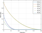
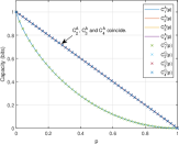
Figure 3: Analytical and Numerical results for the first (left) and second (right) examples in Section VIII-A. In each case, we compute the optimal rate (capacity) with $150$ iterations for each point.

In Fig. 3, we plot the curve of the rate-distortion function and the capacity with respect to the parameter $p$ given by analytical results (superscript $A$) as well as points computed by our algorithms (superscript $C$). We observe that the points computed by the algorithm almost exactly lie on the analytical curve, which shows the accuracy of our algorithm. Considering the number of iterations for each point is relatively limited ($150$ steps), the efficiency of our algorithm is also illustrated.

VIII-B Applications to Problems without Exact Solutions

Consider the rate-distortion and capacity-cost functions for some complex scenarios. In these cases, analytical solutions have not been found and our algorithm plays an important role. Compared with some previous work [19], our algorithms can be applied to practical problems with larger scale.

VIII-B1 Rate-distortion functions for another two lossy computing problems

Let $\mathcal{S}_{1}=\{1,2,...,6\}$, $\mathcal{S}_{2}=\{1,2,3,4\}$, $p(i,j)=\frac{1}{24},\forall i,j$. The most common sum function $f(s_{1},s_{2})=s_{1}+s_{2}$ for the first example and a general nonlinear function $f(s_{1},s_{2})=s_{1}s_{2}-s_{2}+5$ for the second example. We set $\mathcal{Z}=\hat{\mathcal{Z}}=\{2,3,...,10\}$ for the first one and $\mathcal{Z}=\hat{\mathcal{Z}}=\{5,...,25\}$ for the second one. In both examples, the distortion measure $d$ is set to be the quadratic distortion.

Our algorithm computes the rate-distortion functions for $50$ different $D$ and reconstructs the curves. The rate-distortion curves for both examples are depicted in Fig.4. It is also rather convenient for our algorithm to adjust the computational granularity of any parts of the curves.

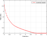
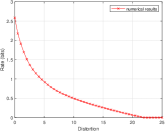
Figure 4: Numerical results for the first (left) and second (right) examples in Section VIII-B1. In each case, we choose $50$ points from the intervals uniformly and compute the corresponding optimal rate with $1000$ iterations.

VIII-B2 Capacity-cost function for the Gaussian additive channel with quantized state information

We consider the channel

$$Y=X+S+Z,$$ (58)

where the channel state $S\sim\mathrm{N}(0,\frac{1}{2})$ and the noise $Z\sim\mathrm{N}(0,1)$ are independent. $S$ can also be used to model the channel input of the other terminal in a Gaussian MAC. In this case, one of the encoders optimizes its input distribution in order to maximize its capacity, on the condition that the input distribution of the other is fixed.

A more practical situation is that $S$ is measured with a given degree of accuracy, so that a quantized version of $S$ instead of $S$ itself is known by the encoder. More formally, let

$$Q_{4}(s)=\mathrm{sgn}(s)(1.5\cdot\mathds{1}\{|s|>1\}+0.5\cdot\mathds{1}\{|s|\leq 1\})$$ (59)

be the quantization function and $S_{1}=Q_{4}(S/\sqrt{\frac{1}{2}})$ be the two-bit quantized state information.

We perform uniform quantization of $X$ and $Y$ over intervals $[-4,4]$ and $[-8,8]$, respectively. Also, $|X|=2^{b}$ and $|Y|=2^{b+1}$, which means there are $b$ bits to represent the input $X$ and $b+1$ bits to express the output $Y$. The transition probability $Y|(X_{s_{1}})_{s_{1}\in\mathcal{S}_{1}},S_{1}$ is computed by the $5$-point closed Newton-Cotes quadrature rule applied on the probability density function, since the density of $S+Z$ can be expressed through the Q-function.

The capacity-cost function for $b=3,4$ is plotted in Fig. 5. Note that the writing on dirty paper scheme gives a capacity $\frac{1}{2}\log(1+B)$ when $S$ is fully gotten by the encoder. Thus it gives an upper bound for the capacity with the quantized side information computed here.

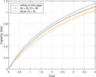
Figure 5: Numerical results for the channel problem with quantized side information in Section VIII-B2. Capacity-cost curves for two quantization schemes with different granularity are plotted. In each case, $50$ points are chosen from the intervals uniformly and the corresponding capacity is computed with $1000$ iterations. The capacity-cost curve of the writing on dirty scheme is also plotted as an upper bound.

VIII-C The Speed-up Effects of Deflation Techniques

The computational time and the differences of the computed optimal rates before and after deflation techniques are summarized in Table III. The deflation period $k$ is set to be $5$ and the criterion is set to be $p^{(n)}(u)<10^{-2}/|\mathcal{U}|$. The number of iterations is $1000$ for the first two examples in Section VIII-B1 and $2000$ for the last example for $b=3,4,5$ in Section VIII-B2 to ensure enough accuracy. To eliminated the effect of noise, the listed time is averaged over $50$ experiments.

We find that the additional deflation techniques only incur a small difference for the computed results. Since the original algorithm is bound to converge, so does the accelerated one. The speed-up ratio becomes larger as the size of the problems increases. It makes the computational time admissible for some cases, which is shown by the last two lines of Table III. It is not surprising that the speed-up effect is more significant for lossy computing problems than for channel coding problems with state, since the cardinality bounds for the former are tighter.

TABLE III: The Computational Time and Error before and after Adding Deflation Techniques for Some Examples

Examples		$(L,T(L))$	Time (s)		Speed-up	Speed-up
			before	after	Ratio	penalty
Sum		$(0.5,1.1503)$	$8.074$	$0.092$	$87.77$	$1.6010-16$
computation		$(2.5,0.1107)$	$4.912$	$0.125$	$39.39$	$1.4410-15$
Nonlinear		$(0.5,2.1827)$	$481.1$	$1.754$	$274.3$	$8.8810-16$
function		$(5.0,0.9295)$	$175.2$	$1.820$	$96.26$	$9.9710-9$
computation		$(20.0,0.0652)$	$172.5$	$3.948$	$43.69$	$1.1110-8$
Gaussian	$|X|=8$	$(1.5,0.5615)$	$8.472$	$0.389$	$21.78$	$3.3210-10$
channel	$|Y|=16$	$(5.0,1.1414)$	$8.397$	$0.333$	$25.22$	$2.9610-13$
with	$|X|=16$	$(1.5,0.6237)$	$285.0$	$6.889$	$41.37$	$3.1610-9$
quantized	$|Y|=32$	$(5.0,1.2066)$	$279.9$	$6.509$	$43.00$	$2.4310-9$
state	$|X|=32$	$(1.5,0.6321)$	-	$174.6$	-	-
information	$|Y|=64$	$(5.0,1.2238)$	-	$162.2$	-	-

The typical trend of time and error during iterations is described by Table IV. The first case is to compute $R(5.0)$ for the nonlinear function computation problem in Section VIII-B1 and the second case is to compute $C(1.5)$ for the channel with quantized state information in Section VIII-B2, where we set $b=4$. The true value is estimated through $1600000$ iterations until the computed result converges to a sufficiently high accuracy. Again the time is averaged over $50$ experiments. Note that the time for $0$ iteration is purely used for initialization.

The numerical experiments verify our discussions in Section VII-E, since each iteration becomes rather cheap after the first few dozens. If we want to compute the rate to a high accuracy, thousands of iterations can be applied and the computational cost is very low. Such strategy can preserve the accuracy because the computed result after deflation techniques closely follow which before such techniques. The cost is almost unaffordable if not aided by deflation techniques.

TABLE IV: The Time and Error of Different Number of Iterations with Deflations

Examples		$0$	$30$	$60$	$125$	$250$	$500$	$1000$	$2000$
Nonlinear	Time (s)	$0.184$	$1.437$	$1.537$	$1.654$	$1.728$	$1.761$	$1.820$	$1.907$
Function	Error	-	$6.4210-2$	$3.2910-2$	$1.3510-2$	$3.9010-3$	$9.2210-4$	$2.7510-4$	$6.6110-5$
Gaussian	Time (s)	$1.865$	$4.979$	$5.679$	$6.184$	$6.543$	$6.612$	$6.719$	$6.889$
channel	Error	-	$8.2810-2$	$3.5310-2$	$1.2810-2$	$3.8910-3$	$9.4910-4$	$1.8410-4$	$3.1210-5$

These results demonstrate the deflation techniques largely reduce computational time without loss of accuracy.

IX Conclusion

In this paper, we systematically studied the lossy computing and channel coding problems through a unified graph-based approach. Interesting reductions for some special cases were derived by our graph-based characterizations. Also, we developed efficient algorithms for the computation of rate-distortion and capacity-cost functions with a given distortion or cost. The algorithms were proved to be convergent and accelerated by heuristic deflation techniques. Applying graph methods and algorithms to more practical problems would be one direction for further work.

Appendix A Proof of Lemma 3 and 4

Proof:

First we show (12) is a convex optimization problem. We only need to verify the convexity of the objective function $GD_{\mathscr{E}}(\bm{q}||\bm{r})$.

Let $(\bm{q}_{1},\bm{r}_{1})$ and $(\bm{q}_{2},\bm{r}_{2})$ be two feasible solutions and $0<\alpha<1$. By the log-sum inequality, we have

$$[(1-\alpha)q_{1}(u|v)+\alpha q_{2}(u|v)]\log\frac{(1-\alpha)q_{1}(u|v)+\alpha q_{2}(u|v)}{(1-\alpha)r_{1}(u|w)+\alpha r_{2}(u|w)}$$

$$\leq(1-\alpha)q_{1}(u|v)\log\frac{q_{1}(u|v)}{r_{1}(u|w)}+\alpha q_{2}(u|v)\log\frac{q_{2}(u|v)}{r_{2}(u|w)}.$$

Multiplying both sides by $p(v)p(w|u,v)$ and taking the sum over all $(u,v)\in\mathscr{E}$ and $w\in\mathcal{W}$, we have

$$GD_{\mathscr{E}}((1-\alpha)\bm{q}_{1}+\alpha\bm{q}_{2}||(1-\alpha)\bm{r}_{1}+\alpha\bm{r}_{2})$$

$$\leq(1-\alpha)GD_{\mathscr{E}}(\bm{q}_{1}||\bm{r}_{1})+\alpha GD_{\mathscr{E}}(\bm{q}_{2}||\bm{r}_{2}).$$

Next we show (3) is convex and we only need to demonstrate its objective function $\mathcal{O}(\bm{p})$ is convex. From Lemma 2,

$$\begin{split}\mathcal{O}(\bm{q})=GD_{\mathscr{E}}(\bm{q}||\bm{q})=\min_{\bm{r}}GD_{\mathscr{E}}(\bm{q}||\bm{r}).\end{split}$$ (60)

We have shown $GD_{\mathscr{E}}(\bm{q}||\bm{r})$ is convex in $(\bm{q},\bm{r})$. $\mathcal{O}(\bm{q})$ is the minimum of $GD_{\mathscr{E}}(\bm{q}||\bm{r})$ with respect to $\bm{r}$, so it is also convex. ∎

Proof:

Consider the problem (3). Since the feasible region expands as $L$ increases, the optimal value $T(L)$ is decreasing in $D$.

Let $\bm{q}_{1}$ and $\bm{q}_{2}$ be two feasible solutions of (3) for $L_{1}$ and $L_{2}$, respectively. Let $\alpha\in(0,1)$. Since the constraints are only linear, $(1-\alpha)\bm{q}_{1}+\alpha\bm{q}_{2}$ is a feasible solution for $(1-\alpha)L_{1}+\alpha L_{2}$. Also, by Lemma 3 and the definition of $T(L)$,

$$T((1-\alpha)L_{1}+\alpha L_{2})\leq\mathcal{O}((1-\alpha)\bm{q}_{1}+\alpha\bm{q}_{2})$$

$$\leq(1-\alpha)\mathcal{O}(\bm{q}_{1})+\alpha\mathcal{O}(\bm{q}_{2}).$$

Since the choice of $\bm{q}_{1}$ and $\bm{q}_{2}$ is arbitrary, then we have

$$T((1-\alpha)L_{1}+\alpha L_{2})\leq(1-\alpha)T(L_{1})+\alpha T(L_{2}),$$

which gives the convexity of $T(L)$. ∎

Appendix B Proof of Proposition 1

Let

$$L^{\prime}_{max}=\min_{u\in\mathcal{U}}\left\{\sum_{v}p(v)\tilde{l}(v,u)\right\}.$$

For $D\geq L^{\prime}_{max}$, let $u_{0}$ be one of the elements in $\mathcal{U}$ such that

$$\sum_{v}p(v)\tilde{l}(v,u_{0})=\min_{u^{\prime}\in\mathcal{U}}\left\{\sum_{v}p(v)\tilde{l}(v,u^{\prime})\right\}.$$

Then it is easy to see that $p(u|s_{1})=\mathds{1}{(u=u_{0})}$ is a feasible solution, such that the value of the objective function is $0$. Also, by monotonicity $R(D)=0$ for $D\geq D_{max}$.

Now assume that $R(D)=0$. Since the feasible region is always compact, there exists some $p(u|v)$ such that $I(U;V|W)=I(U;V)-I(U;W)=0$. Then $U$ and $V$ are conditional independent given $Y$. Since $U-V-W$ is a Markov chain, $p(u|v)=p(u),\forall v$. So we have

$$\mathbb{E}[\hat{l}(V,U,W)]=\sum_{u}p(u)\sum_{v,w}p(v,w)\hat{l}(v,u,w)$$

$$\geq \sum_{u}p(u)\min_{u^{\prime}\in\mathcal{U}}\left\{\sum_{v}p(v)\tilde{l}(v,u^{\prime})\right\}$$

$$= \min_{u^{\prime}\in\mathcal{U}}\left\{\sum_{v}p(v)\tilde{l}(v,u^{\prime})\right\}=L^{\prime}_{max}.$$

Thus we have $R(D)=0$ if and only if $D\geq L^{\prime}_{max}$. By the definition of $L_{max}$, $L_{max}=L^{\prime}_{max}$.

Appendix C Proof of Lemma 6

We first show $\omega_{\bm{p}^{\prime}}$ is a feasible weight. For any $v\in\mathcal{V}_{k}$,

$$\sum_{u^{\prime}\in\mathscr{E}_{v}^{\prime}}p(u^{\prime}|v) =\sum_{u^{\prime}\in\mathscr{E}^{\prime}_{v}}\sum_{\begin{subarray}{c}u\in\mathscr{E}_{v}\\ h_{k}(u)=u^{\prime}\end{subarray}}p(u^{\prime}|v)$$

$$=\sum_{u\in\mathscr{E}_{v}}p(u|v)=1.$$

By (24), we always have $\tilde{l}(u^{\prime},v)\leq\tilde{l}(v,u)$ if $v\in\mathcal{V}_{k}$, $(v,u^{\prime})\in\mathscr{E}^{\prime}$ and $h_{k}(u)=u^{\prime}$. so

$$Loss(\bm{p^{\prime}})=\sum_{\begin{subarray}{c}k,v\in\mathcal{V}_{k},\\ (v,u^{\prime})\in\mathscr{E}^{\prime}\end{subarray}}p(v)p^{\prime}(u^{\prime}|v)\tilde{l}(u^{\prime},v)$$

$$\leq \sum_{\begin{subarray}{c}k,v\in\mathcal{V}_{k},\\ (v,u^{\prime})\in\mathscr{E}^{\prime}\end{subarray}}\sum_{\begin{subarray}{c}u\in\mathscr{E}_{v}\\ h_{k}(u)=u^{\prime}\end{subarray}}p(v)p(u|v)\tilde{l}(v,u)=Loss(\bm{p})$$

is by (23) and (26).

It remains to show such an operation does not increase $\mathcal{O}(\bm{p})$. For any $w\in\mathcal{W}_{k}$, by (23), (25) and (26) we have

$$p^{\prime}(u^{\prime},w)=\sum_{\begin{subarray}{c}v\in\mathcal{V}_{k}\\ (v,u^{\prime})\in\mathscr{E}^{\prime}\end{subarray}}p(v)p^{\prime}(u^{\prime}|v)p(w|u^{\prime},v)$$

$$= \sum_{\begin{subarray}{c}v\in\mathcal{V}_{k}\\ (v,u^{\prime})\in\mathscr{E}^{\prime}\end{subarray}}\sum_{\begin{subarray}{c}u\in\mathscr{E}_{v}\\ h_{k}(u)=u^{\prime}\end{subarray}}p(v)p(u|v)p(w|u,v)$$

$$= \sum_{\begin{subarray}{c}u:h_{k}(u)=u^{\prime}\end{subarray}}\sum_{v:(v,u)\in\mathscr{E}}p(v)p(u|v)p(w|u,v)$$

$$= \sum_{u:h_{k}(u)=u^{\prime}}p(u,w),$$

which implies $p^{\prime}(u^{\prime}|w)=\sum_{u:h_{k}(u)=u^{\prime}}p(u|w)$. Then by (23), (25) and (26) we have

$$\mathcal{O}(\bm{p^{\prime}})-\mathcal{O}(\bm{p})$$

$$= \sum_{\begin{subarray}{c}k,v\in\mathcal{V}_{k},\\ w\in\mathcal{W}_{k},\\ (v,u^{\prime})\in\mathscr{E}^{\prime}\end{subarray}}\sum_{\begin{subarray}{c}u:\\ h_{k}(u)=u^{\prime}\end{subarray}}p(v)p(u|v)p(w|u^{\prime},v)\log\frac{p(u|w)p^{\prime}(u^{\prime}|v)}{p(u|v)p^{\prime}(u^{\prime}|w)}$$

$$\leq \sum_{\begin{subarray}{c}k,v\in\mathcal{V}_{k},\\ w\in\mathcal{W}_{k},\\ (v,u^{\prime})\in\mathscr{E}^{\prime}\end{subarray}}\sum_{\begin{subarray}{c}u:\\ h_{k}(u)=u^{\prime}\end{subarray}}p(v)p(u|v)p(w|u^{\prime},v)\frac{p(u|w)p^{\prime}(u^{\prime}|v)}{p(u|v)p^{\prime}(u^{\prime}|w)}-1$$

$$= \sum_{\begin{subarray}{c}k,v\in\mathcal{V}_{k},\\ w\in\mathcal{W}_{k},\\ (v,u^{\prime})\in\mathscr{E}^{\prime}\end{subarray}}p(v)p^{\prime}(u^{\prime}|w)p(w|u^{\prime},v)-1=0,$$

finishing the proof.

Appendix D Proof of Lemma 2, Theorem 9, 3 and 11

The following lemma characterizes the decreasing value of the partial minimization processes. The proof is by direct calculation.

Lemma 11.

We have the following identities for $\bm{q}$ with $\mathrm{supp}(\bm{q})\subseteq\mathscr{E}$, where the generalized K-L divergence for $q(u|v)$ and $r(u|w)$ are naturally defined as

$$GD_{\mathscr{E}}(\bm{q}_{1}||\bm{q}_{2})=\sum_{(v,u)\in\mathscr{E}}p(v)q_{1}(u|v)\log\frac{q_{1}(u|v)}{q_{2}(u|v)}$$

and

$$GD_{\bm{q}}(\bm{r}_{1}||\bm{r}_{2})=\sum_{u,w}q(w)r_{1}(u|w)\log\frac{r_{1}(u|w)}{r_{2}(u|w)},$$

where $q(w)\triangleq\sum_{v,u}p(v)q(u|v)p(w|u,v)$.

$$F_{s}(\bm{q},\bm{r})=F_{s}(\bm{q}_{s}^{*}(\bm{r}),\bm{r})+GD_{\mathscr{E}}(\bm{q}||\bm{q}_{s}^{*}(\bm{r})),$$ (61)

$$F_{s}(\bm{q},\bm{r})=F_{s}(\bm{q},\bm{r}^{*}(\bm{q}))+GD_{\bm{q}}(\bm{r}^{*}(\bm{q})||\bm{r}).$$ (62)

Also we have

$$GD_{\mathscr{E}}(\bm{q}_{s}^{*}(\bm{r})||\bm{r})=-s\cdot Loss(\bm{q}_{s}^{*}(\bm{r}))$$ (63)

$$-\sum_{v}p(v)\log\sum_{u^{\prime}\in\mathscr{E}_{v}}e^{-s\tilde{l}(v,u^{\prime})}\prod_{w^{\prime}}r(u^{\prime}|w^{\prime})^{p(w^{\prime}|u^{\prime},v)}.$$

Proof:

Immediately from  (62). ∎

The partial minimization for $\bm{q}$ depends on $s$, the next corollary describe the behavior of the penalty function with parameter $s$ while doing the minimization for a different parameter $s^{\prime}$.

Corollary 5.

$$F_{s}(\bm{q},\bm{r})=F_{s}(\bm{q}_{s^{\prime}}^{*}(\bm{r}),\bm{r})+GD_{\mathscr{E}}(\bm{q}||\bm{q}_{s^{\prime}}^{*}(\bm{r}))$$ (64)

$$+(s-s^{\prime})\left[Loss(\bm{q})-Loss(\bm{q}_{s^{\prime}}^{*}(\bm{r}))\right].$$

Proof:

By the identity $F_{s}(\bm{q},\bm{r})=F_{s^{\prime}}(\bm{q},\bm{r})+(s-s^{\prime})Loss(\bm{q})$ and Lemma 11. ∎

Corollary 6.

The conditional distribution pair $(\bm{q}^{0},\bm{r}^{0})$ minimizing the penalty function $F_{s^{*}}(\bm{q},\bm{r})$ exists and satisfies $\bm{q}_{s^{*}}^{*}(\bm{r}^{0})=\bm{q}^{0}$. Also, $r^{*}(\bm{q}^{0})(\cdot|w)=r^{0}(\cdot|w)$ for any $w$ such that $q^{0}(w)>0$.

Proof:

The domain of $(\bm{q},\bm{r})$ is compact and $F_{s^{*}}(\bm{q},\bm{r})$ is continuous, so there exists conditional distribution pair $(\bm{q}^{0},\bm{r}^{0})$ minimizing the penalty function $F_{s^{*}}(\bm{q},\bm{r})$.

Then by the definition of $(\bm{q}^{0},\bm{r}^{0})$,

$$F_{s^{*}}(\bm{q}^{0},\bm{r}^{0})\leq F_{s^{*}}(\bm{q}_{s^{*}}^{*}(\bm{r}^{0}),\bm{r}^{0}),$$

$$F_{s^{*}}(\bm{q}^{0},\bm{r}^{0})\leq F_{s^{*}}(\bm{q}^{0},\bm{r}^{*}(\bm{q}^{0})).$$

So by Lemma 11 we have $GD_{\mathscr{E}}(\bm{q}^{0}||\bm{q}_{s^{*}}^{*}(\bm{r}^{0}))=0$ and $GD(\bm{r}^{*}(\bm{q}^{0})||\bm{r}^{0})=0$.

By (4) we always have $\bm{q}_{s^{*}}^{*}(\bm{r}^{0})=\bm{q}^{0}$. Similarly, $r^{*}(\bm{q}^{0})(\cdot|w)=r^{0}(\cdot|w)$ for any $w$ such that $q^{0}(w)>0$. ∎

Proposition 2.

During the iterations of Algorithm 1 ,

$$F_{s^{*}}(\bm{q}^{(n)},\bm{r}^{(n)})\leq F_{s^{*}}(\bm{q}^{(n)},\bm{r}^{(n-1)}).$$ (65)

If either $s^{n}=s^{*},\forall n$ or for some $(\bm{q}^{0},\bm{r}^{0})\in\arg\min_{\bm{q},\bm{r}}F_{s^{*}}(\bm{q},\bm{r})$, $Loss(\bm{q}^{(n)})=Loss(\bm{q}^{0}),\forall n$ holds (for Algorithm 1 with $\Delta_{n}(\bm{q}^{0})=0$), then we have

$$F_{s^{*}}(\bm{q}^{(n+1)},\bm{r}^{(n)})\leq F_{s^{*}}(\bm{q}^{(n)},\bm{r}^{(n)})\leq F_{s^{*}}(\bm{q}^{(n)},\bm{r}^{(n-1)}).$$ (66)

Proof:

By Lemma 11, we have

$$F_{s^{*}}(\bm{q}^{(n)},\bm{r}^{(n-1)})$$

$$= F_{s^{*}}(\bm{q}^{(n)},\bm{r}^{*}(\bm{q}^{(n)}))+GD_{\bm{q}^{(n)}}(\bm{r}^{*}(\bm{q}^{(n)})||\bm{r}^{(n-1)})$$

$$= F_{s^{*}}(\bm{q}^{(n)},\bm{r}^{(n)})+GD_{\bm{q}^{(n)}}(\bm{r}^{(n)}||\bm{r}^{(n-1)})\geq F_{s^{*}}(\bm{q}^{(n)},\bm{r}^{(n)}).$$

Furthermore, if either $s^{n}=s^{*},\forall n$ or $Loss(\bm{q}^{(n)})=L^{*},\forall n$ holds, then since $\bm{q}_{s^{(n)}}^{*}(\bm{r}^{(n)})=\bm{q}^{(n+1)}$,

$$F_{s^{*}}(\bm{q}^{(n)},\bm{r}^{(n)})=F_{s^{*}}(\bm{q}^{(n+1)},\bm{r}^{(n)})+GD_{\mathscr{E}}(\bm{q}^{(n)}||\bm{q}^{(n+1)})$$

$$+ (s^{*}-s^{(n)})(Loss(\bm{q}^{(n)})-Loss(\bm{q}^{(n+1)}))$$

$$= F_{s^{*}}(\bm{q}^{(n+1)},\bm{r}^{(n)})+GD_{\mathscr{E}}(\bm{q}^{(n)}||\bm{q}^{(n+1)})$$

$$\geq F_{s^{*}}(\bm{q}^{(n+1)},\bm{r}^{(n)}).$$

∎

Lemma 12.

For some $(\bm{q}^{0},\bm{r}^{0})\in\arg\min_{\bm{q},\bm{r}}F_{s^{*}}(\bm{q},\bm{r})$, define

$$\Gamma_{n}(\bm{q}^{0})=GD_{\mathscr{E}}(\bm{q}^{0}||\bm{q}^{(n)})-GD_{\bm{q}^{0}}(\bm{r}^{0}||\bm{r}^{(n)}),$$

then $\Gamma_{n}(\bm{q}^{0})\geq 0$. Also, we have

$$F_{s^{*}}(\bm{q}^{(n)},\bm{r}^{(n-1)})-F_{s^{*}}(\bm{q}^{0},\bm{r}^{0})+\Gamma_{n-1}(\bm{q}^{0})+\Delta_{n}(\bm{q}^{0})$$ (67)

$$= GD_{\mathscr{E}}(\bm{q}^{0}||\bm{q}^{(n-1)})-GD_{\mathscr{E}}(\bm{q}^{0}||\bm{q}^{(n)}).$$

Proof:

By the definition of $\Gamma_{n}(\bm{q}^{0})$, $\bm{r}^{0}$ and $\bm{r}^{(n)}$,

$$\Gamma_{n}(\bm{q}^{0}) =-\sum_{v,u,w}p(v)q^{0}(u|v)p(w|u,v)\log\frac{q^{(n)}(u|v)r^{0}(u|w)}{q^{0}(u|v)r^{(n)}(u|w)}$$

$$\geq-\sum_{v,u,w}p(v)q^{0}(u|v)p(w|u,v)\left(\frac{q^{(n)}(u|v)r^{0}(u|w)}{q^{0}(u|v)r^{(n)}(u|w)}-1\right)$$

$$=-\sum_{u,w}\sum_{v}p(v)p(w|u,v)\frac{q^{(n)}(u|v)r^{0}(u|w)}{r^{(n)}(u|w)}+1$$

$$=-\sum_{u,w}r^{0}(u|w)\sum_{u^{\prime},v^{\prime}}p(v^{\prime})p(w|u^{\prime},v^{\prime})q^{(n)}(u^{\prime}|v^{\prime})+1=0.$$

Since $Loss(\bm{q}^{0})=L^{*}$ and $Loss(\bm{q}^{(n)})=G_{\bm{r}^{(n-1)}}(s^{(n)})$, by Corollary 5 we have

$$F_{s^{*}}(\bm{q}^{0},\bm{r}^{(n-1)})=F_{s^{*}}(\bm{q}^{(n)},\bm{r}^{(n-1)})+GD_{\mathscr{E}}(\bm{q}^{0}||\bm{q}^{(n)})$$ (68)

$$+(s^{(n)}-s^{*})(G_{\bm{r}^{(n-1)}}(s^{(n)})-Loss(\bm{q}^{0})).$$

Note that by Corollary 6, $\bm{r}^{0}=\bm{r}^{*}(\bm{q}^{0})$. Then by Lemma 11 we have

$$F_{s^{*}}(\bm{q}^{0},\bm{r}^{(n-1)})=F_{s^{*}}(\bm{q}^{0},\bm{r}^{0})+GD_{\bm{q}^{0}}(\bm{r}^{0}||\bm{r}^{(n-1)}).$$ (69)

By (68) and (69) we have finished the proof. ∎

Proof:

Consider the first part and suppose $(\bm{q}^{0},\bm{r}^{0})\in\arg\min_{\bm{q},\bm{r}}F_{s^{*}}(\bm{q},\bm{r})$. By Lemma 12, we take the sum and get

$$\sum_{k=n+1}^{m}\left(F_{s^{*}}(\bm{q}^{(k)},\bm{r}^{(k-1)})-F_{s^{*}}(\bm{q}^{0},\bm{r}^{0})+\Gamma_{k-1}(\bm{q}^{0})+\Delta_{k}(\bm{q}^{0})\right)$$ (70)

$$=GD_{\mathscr{E}}(\bm{q}^{0}||\bm{q}^{(n)})-GD_{\mathscr{E}}(\bm{q}^{0}||\bm{q}^{(m)}),$$

for $m>n\geq 1$. Take $n=1$ and we can obtain

$$\begin{split}&\sum_{k=2}^{m}\left(F_{s^{*}}(\bm{q}^{(k)},\bm{r}^{(k-1)})-F_{s^{*}}(\bm{q}^{0},\bm{r}^{0})+\Gamma_{k-1}(\bm{q}^{0})+\Delta_{k}(\bm{q}^{0})\right)\\ \leq&GD_{\mathscr{E}}(\bm{q}^{0}||\bm{q}^{(1)})\leq\log|\mathcal{U}|,\end{split}$$

which is because $q^{(1)}(u|y)=\frac{1}{|\mathcal{U}|}$. Let $m\to\infty$, then

$$\sum_{k=2}^{\infty}\left(F_{s^{*}}(\bm{q}^{(k)},\bm{r}^{(k-1)})-F_{s^{*}}(\bm{q}^{0},\bm{r}^{0})\right)\leq\log|\mathcal{U}|$$ (71)

Each term in the sum is nonnegative, so

$$\lim_{k\to\infty}F_{s^{*}}(\bm{q}^{(k)},\bm{r}^{(k-1)})=F_{s^{*}}(\bm{q}^{0},\bm{r}^{0}).$$

Also, $\lim_{k\to\infty}F_{s^{*}}(\bm{q}^{(k)},\bm{r}^{(k)})=F_{s^{*}}(\bm{q}^{0},\bm{r}^{0})=\min_{\bm{q},\bm{r}}F_{s^{*}}(\bm{q},\bm{r})$ by (65). It proves the first part.

Then we consider the second part. $\{\bm{q}^{(n)}\}_{n\geq 1}$ is a sequence in a compact set, and hence has a convergent subsequence, donoted by $\{\bm{q}^{(n_{k})}\}_{k=1}^{\infty}$. Let $\bm{q}^{(0)}$ be its limit, and let $\bm{r}^{(0)}=\bm{r}^{*}(\bm{q}^{(0)})$. Then $\bm{r}^{(n_{k})}=\bm{r}^{*}(\bm{q}^{(n_{k})})$ and

$$\lim_{k\to\infty}F_{s^{*}}(\bm{q}^{(n_{k})},\bm{r}^{(n_{k})})=\lim_{k\to\infty}F_{s^{*}}(\bm{q}^{(n_{k})},\bm{r}^{*}(\bm{q}^{(n_{k})}))$$

$$= F_{s^{*}}(\bm{q}^{(0)},\bm{r}^{*}(\bm{q}^{(0)}))=F_{s^{*}}(\bm{q}^{(0)},\bm{r}^{(0)}),$$

which implies $F_{s^{*}}=\min_{\bm{q},\bm{r}}F_{s^{*}}(\bm{q},\bm{r})$. Also, we have

$$Loss(\bm{q}^{(0)})=\lim_{n\to\infty}Loss(\bm{q}^{(n_{k})}),$$

and hence $\bm{q}^{(0)}$ satisfies the corresponding constraint in one of the three problems. So $(\bm{q}^{(0)},\bm{r}^{(0)})$ is an optimal solution for the corresponding problem, which implies that (70) is still satisfied when $(\bm{q}^{0},\bm{r}^{0})$ is replaced by $(\bm{q}^{(0)},\bm{r}^{(0)})$.

By the version of (70) where $(\bm{q}^{0},\bm{r}^{0})$ is replaced by $(\bm{q}^{(0)},\bm{r}^{(0)})$, we have $GD_{\mathscr{E}}(\bm{q}^{(0)}||\bm{q}^{(n)})$ is decreasing. Since we have $\lim_{k\to\infty}\bm{q}^{(n_{k})}=\bm{q}^{(0)}$, then we have $\lim_{k\to\infty}GD_{\mathscr{E}}(\bm{q}^{(0)}||\bm{q}^{(n_{k})})=0$ and hence $\lim_{n\to\infty}GD_{\mathscr{E}}(\bm{q}^{(0)}||\bm{q}^{(n)})=0$. So $\bm{q}^{(n)}\to\bm{q}^{(0)}$, which implies $\bm{r}^{(n)}\to\bm{r}^{(0)}$ as $n\to\infty$. In other words, the solutions $(\bm{q}^{(n+1)},\bm{r}^{(n)})$ generated by Algorithm 1 converge to an optimal solution $(\bm{q}^{(0)},\bm{r}^{(0)})$ for the corresponding problem.

For the case when $\Delta_{n}(\bm{q}^{0})=0$, by (66) $F_{s^{*}}(\bm{q}^{(n+1)},\bm{r}^{(n)})-F_{s^{*}}(\bm{q}^{0},\bm{r}^{0})$ is decreasing and hence it is no greater than $\frac{\log|\mathcal{U}|}{n}$ by (71). By (65) we finish the proof. ∎

Appendix E Proof of Theorem 10

The case for $L\in(L_{min},L_{Max})$ is contained in Theorem 9. It remains to consider the case for $L=L_{min}$ or $L\geq L_{Max}$ and we only list the skeleton results which are slightly different from which in Appendix D.

Lemma 13.

The following holds for $\bm{q}$ with $\mathrm{supp}(\bm{q})\subseteq\mathscr{E}$,

$$GD_{\mathscr{E}}(\bm{q}||\bm{r})=GD_{\mathscr{E}}(\bm{q}_{0}^{*}(\bm{r})||\bm{r})+GD_{\mathscr{E}}(\bm{q}||\bm{q}_{0}^{*}(\bm{r})),$$ (72)

$$GD_{\mathscr{E}}(\bm{q}||\bm{r})=GD_{\mathscr{E}}(\bm{q}||\bm{r}^{*}(\bm{q}))+GD_{\bm{q}}(\bm{r}^{*}(\bm{q})||\bm{r}).$$ (73)

Proposition 3.

During the iterations of Algorithm 2 for $L=L_{min}$ or $L\geq L{Max}$,

$$GD_{\mathscr{E}}(\bm{q}^{(n+1)},\bm{r}^{(n)})\leq GD_{\mathscr{E}}(\bm{q}^{(n)},\bm{r}^{(n)})$$ (74)

$$\leq GD_{\mathscr{E}}(\bm{q}^{(n)},\bm{r}^{(n-1)}).$$

Lemma 14.

Let $(\bm{q}^{0},\bm{r}^{0})\in\arg\min_{\bm{q},\bm{r}}GD_{\mathscr{E}}(\bm{q}||\bm{r})$ and define

$$\tilde{\Gamma}_{n}(\bm{q}^{0})=GD_{\mathscr{E}}(\bm{q}^{0}||\bm{q}^{(n)})-GD_{\bm{q}^{0}}(\bm{r}^{0}||\bm{r}^{(n)}),$$

then $\Gamma_{n}(\bm{q}^{0})\geq 0$. Also, we have

$$GD_{\mathscr{E}}(\bm{q}^{(n)}||\bm{r}^{(n-1)})-GD_{\mathscr{E}}(\bm{q}^{0}||\bm{r}^{0})+\tilde{\Gamma}_{n-1}(\bm{q}^{0})$$ (75)

$$= GD_{\mathscr{E}}(\bm{q}^{0}||\bm{q}^{(n-1)})-GD_{\mathscr{E}}(\bm{q}^{0}||\bm{q}^{(n)}).$$

Proof:

Note that the choice of initial value guarantees that $GD_{\mathscr{E}}(\bm{q}^{0}||\bm{q}^{(1)})\leq\infty$, so the proof is by similar arguments as for Theorem 9. ∎

Appendix F Proof of Lemma 10

Let $U$ be a feasible random variable with distribution $p(u)$ for (3). With fixed $p(v,w|u)$, we construct another feasible random variable $U^{\prime}$ with distribution $\tilde{p}(u)$, satisfying the property above.

Note that

$$H(W|U)-H(V|U)$$

$$=\sum_{u}p(u)(H(W|U=u)-H(V|U=u))$$

$$\mathbb{E}[l(v,u,W)]=\sum_{u},p(u)\sum_{v,w}p(v,w|u)l(v,u,w),$$

$$p(v)=\sum_{u}p(u)p(v|u),$$

$$p(w)=\sum_{u}p(u)p(w|u).$$

If we want to fix $H(W|U)-H(V|U)$, $\mathbb{E}[l(v,u,W)]$, $p(v),\forall v$ and $p(w),\forall w$, we only need to impose

$$1+1+(|\mathcal{V}|-1)+(|\mathcal{W}|-1)=|\mathcal{V}|+|\mathcal{W}|$$

equations. By the Fenchel–Eggleston–Carathéodory theorem, there exists some $U^{\prime}$ such that there are at most $|\mathcal{V}|+|\mathcal{W}|$ of $u$ which satisfy $\tilde{p}(u)>0$. Also, While $p(u)$ is replaced by $\tilde{p}(u)$, $p(w)$ $p(w|u,v)$ and $p(v)$ are fixed. Hence

$$I(U;V)-I(U;W)=H(V)-H(W)-H(V|U)+H(W|U)$$

is also fixd.

References

• [1] T. Cover and M. Chiang, “Duality between channel capacity and rate distortion with two-sided state information,” IEEE Transactions on Information Theory, vol. 48, no. 6, pp. 1629–1638, Jun. 2002.
• [2] S. Pradhan, J. Chou, and K. Ramchandran, “Duality between source coding and channel coding and its extension to the side information case,” IEEE Transactions on Information Theory, vol. 49, no. 5, pp. 1181–1203, May 2003.
• [3] R. Barron, B. Chen, and G. Wornell, “The duality between information embedding and source coding with side information and some applications,” IEEE Transactions on Information Theory, vol. 49, no. 5, pp. 1159–1180, May 2003.
• [4] S. I. Gel’fand and M. S. Pinsker, “Coding for channel with random parameters,” Probl. Contr. and Inform. Theory, vol. 9, no. 1, pp. 19–31, 1980.
• [5] A. Wyner and J. Ziv, “The rate-distortion function for source coding with side information at the decoder,” IEEE Transactions on Information Theory, vol. 22, no. 1, pp. 1–10, Jan. 1976.
• [6] H. Yamamoto, “Wyner-Ziv theory for a general function of the correlated sources,” IEEE Transactions on Information Theory, vol. 28, no. 5, pp. 803–807, Sep. 1982.
• [7] J. Körner, “Coding of an information source having ambiguous alphabet and the entropy of graphs,” in 6th Prague Conference on Information Theory, etc., Prague, Czech, Sep. 1973, pp. 411–425.
• [8] H. Witsenhausen, “The zero-error side information problem and chromatic numbers,” IEEE Transactions on Information Theory, vol. 22, no. 5, pp. 592–593, Sep. 1976.
• [9] A. Orlitsky and J. Roche, “Coding for computing,” IEEE Transactions on Information Theory, vol. 47, no. 3, pp. 903–917, Mar. 2001.
• [10] V. Doshi, D. Shah, and M. Medard, “Source coding with distortion through graph coloring,” in 2007 IEEE International Symposium on Information Theory, Nice, France, Jun. 2007, pp. 1501–1505.
• [11] V. Doshi, D. Shah, M. Médard, and M. Effros, “Functional compression through graph coloring,” IEEE Transactions on Information Theory, vol. 56, no. 8, pp. 3901–3917, Aug. 2010.
• [12] S. Basu, D. Seo, and L. R. Varshney, “Functional epsilon entropy,” in 2020 Data Compression Conference (DCC), Snowbird, UT, USA, Mar. 2020, pp. 332–341.
• [13] ——, “Hypergraph-based source codes for function computation under maximal distortion,” 2022. [Online]. Available: https://arxiv.org/abs/2204.02586
• [14] R. Blahut, “Computation of channel capacity and rate-distortion functions,” IEEE Transactions on Information Theory, vol. 18, no. 4, pp. 460–473, Jul. 1972.
• [15] S. Arimoto, “An algorithm for computing the capacity of arbitrary discrete memoryless channels,” IEEE Transactions on Information Theory, vol. 18, no. 1, pp. 14–20, Jan. 1972.
• [16] F. Willems, Computation of the Wyner-Ziv rate-distortion function, ser. EUT report. E, Fac. of Electrical Engineering.   Eindhoven: Technische Hogeschool Eindhoven, 1983.
• [17] F. Dupuis, W. Yu, and F. Willems, “Blahut-Arimoto algorithms for computing channel capacity and rate-distortion with side information,” in International Symposium on Information Theory, Chicago, IL, USA, Jun. 2004, p. 179.
• [18] E. Tuncel and K. Rose, “Computation and analysis of the N-layer scalable rate-distortion function,” IEEE Transactions on Information Theory, vol. 49, no. 5, pp. 1218–1230, May 2003.
• [19] S. Cheng, V. Stankovic, and Z. Xiong, “Computing the channel capacity and rate-distortion function with two-sided state information,” IEEE Transactions on Information Theory, vol. 51, no. 12, pp. 4418–4425, Dec. 2005.
• [20] W. Ye, H. Wu, S. Wu, Y. Wang, W. Zhang, H. Wu, and B. Bai, “An optimal transport approach to the computation of the LM rate,” in IEEE Global Communications Conference, Rio de Janeiro, Brazil, Dec. 2022.
• [21] S. Wu, W. Ye, H. Wu, H. Wu, W. Zhang, and B. Bai, “A communication optimal transport approach to the computation of rate distortion functions,” 12 2022. [Online]. Available: https://arxiv.org/abs/2212.10098
• [22] M. Hayashi, “Bregman divergence based em algorithm and its application to classical and quantum rate distortion theory,” IEEE Transactions on Information Theory, vol. 69, no. 6, pp. 3460–3492, Jun. 2023.
• [23] J. Bondy and U. Murty, Graph Theory.   New York: Springer, 2008.
• [24] D. Yuan, T. Guo, B. Bai, and W. Han, “Lossy computing with side information via multi-hypergraphs,” in 2022 IEEE Information Theory Workshop, Mumbai, India, Nov. 2022, pp. 344–349.
• [25] A. El Gamal and Y.-H. Kim, Network Information Theory.   Cambridge: Cambridge University Press, 2011.
• [26] V. Harangi, X. Niu, and B. Bai, “Conditional graph entropy as an alternating minimization problem,” 2022. [Online]. Available: https://arxiv.org/pdf/2209.00283v1