An Efficient Transformer for Simultaneous Learning of BEV and Lane Representations in 3D Lane Detection

Abstract

Accurately detecting lane lines in 3D space is crucial for autonomous driving. Existing methods usually first transform image-view features into bird’s-eye-view (BEV) by aid of inverse perspective mapping (IPM), and then detect lane lines based on the BEV features. However, IPM ignores the changes in road height, leading to inaccurate view transformations. Additionally, the two separate stages of the process can cause cumulative errors and increased complexity. To address these limitations, we propose an efficient transformer for 3D lane detection. Different from the vanilla transformer, our model contains a decomposed cross-attention mechanism to simultaneously learn lane and BEV representations. The mechanism decomposes the cross-attention between image-view and BEV features into the one between image-view and lane features, and the one between lane and BEV features, both of which are supervised with ground-truth lane lines. Our method obtains 2D and 3D lane predictions by applying the lane features to the image-view and BEV features, respectively. This allows for a more accurate view transformation than IPM-based methods, as the view transformation is learned from data with a supervised cross-attention. Additionally, the cross-attention between lane and BEV features enables them to adjust to each other, resulting in more accurate lane detection than the two separate stages. Finally, the decomposed cross-attention is more efficient than the original one. Experimental results on OpenLane and ONCE-3DLanes demonstrate the state-of-the-art performance of our method.

1 Introduction

Lane detection is a crucial component of assisted and autonomous driving systems, as it enables a range of downstream tasks such as route planning, lane keeping assist, and high-definition (HD) map construction [19]. In recent years, deep-learning-based lane detection algorithms have achieved impressive results in 2D image space. However, in practical applications, it is often necessary to represent lane lines in 3D space or bird’s-eye-view (BEV). This is particularly useful for tasks that involve interactions with the environment, such as planning and control.

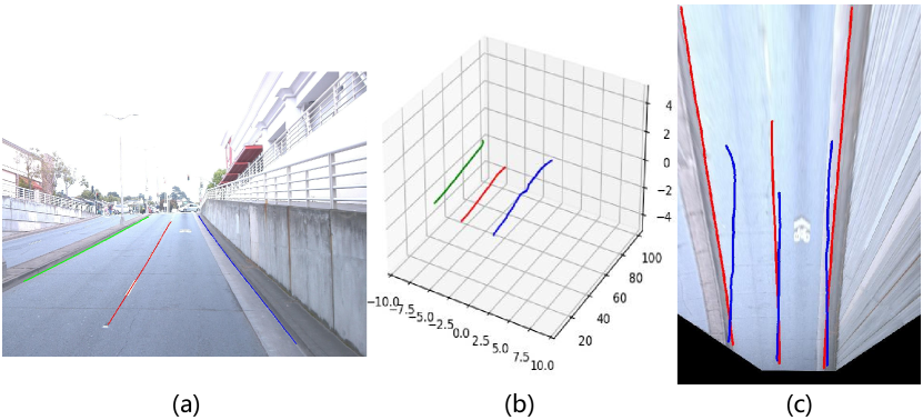
Figure 1: The illustration of lanes lines in different views. (a) The lane lines in image view. (b) The lane lines in 3D space. (c) The lane lines in BEV. The red lane lines in (c) are obtained by projecting those in (a) with IPM. The blue lane lines in (c) are obtained by projecting those in (b) with height collapse.

One typical 3D lane detection pipeline is to first detect lane lines in image view, and then project them into BEV [31, 24, 25, 27, 36]. The projection is usually achieved by inverse perspective mapping (IPM) which assumes a flat road surface. However, as shown in Figure 1, IPM will cause the projected lane lines to diverge or converge in case of uphill or downhill, due to the neglect of the changes in road height. To solve this problem, SALAD [36] predicts the real depth of lane lines along with their image-view positions, and then project them into 3D space with camera in/extrinsics. However, depth estimation is inaccurate at a distance, affecting the projection accuracy.

State-of-the-art methods tend to predict the 3D structure of lane lines directly from BEV [9, 8, 10, 4, 17]. They first transform an image-view feature map into BEV by aid of IPM, and then detect lane lines based on the BEV feature map. However, as shown in Figure 1(c), due to the planar assumption of IPM, the ground-truth 3D lane lines (blue lines) are not aligned with the underlying BEV lane features (red lines), when encountering uneven roads. To solve this problem, some methods [10, 4, 17] represent the ground-truth 3D lane lines in a virtual top-view by first projecting them onto the image plane, and then projecting them onto a flat road plane via IPM (red lines in Fig. 1(c)). Then these methods predict the real height of lane lines along with their positions in the virtual top-view, and finally project them into 3D space with a geometric transformation. However, the accuracy of the predicted heights significantly impacts the transformed BEV positions, which affects the model’s robustness. Moreover, the separate view transformation and lane detection lead to cumulative error and increased complexity.

To overcome these limitations of current methods, we propose an efficient transformer for 3D lane detection. Unlike the vanilla transformer, our model incorporates a decomposed attention mechanism to learn lane and BEV representations simultaneously in a supervised manner. The mechanism decomposes the cross-attention between image-view and BEV features into the one between image-view and lane features, and the one between BEV and lane features. We supervise the decomposed cross-attentions with ground-truth lane lines, where we obtain the 2D and 3D lane predictions by applying the lane features to the image-view and BEV features, respectively.

To achieve this, we generate dynamic kernels for each lane line from the lane features. We then use these kernels to convolve the image-view and BEV feature maps, and obtain the image-view and BEV offset maps, respectively. The offset maps predict the offsets of each pixel to its nearest lane point in 2D and 3D space, which we then process with a voting algorithm to obtain the final 2D and 3D lane points, respectively. Since the view transformation is learned from data with a supervised cross-attention, it is more accurate than the IPM-based ones. Additionally, the lane and BEV features can dynamically adjust to each other with cross-attention, resulting in more accurate lane detection than the two separate stages. Our decomposed cross-attention is more efficient than the vanilla cross attention between image-view and BEV features. The experiments on two benchmark datasets, including OpenLane and ONCE-3DLanes demonstrate the effectiveness and efficiency of our method.

2 Related Work

2.1 3D Lane Detection in Image View

3D lane detection can be achieved in image view. Some methods first detect 2D lane lines in image view, and then project them into bird’s-eye-view (BEV) [31, 24, 25, 27, 36]. There are various methods proposed to tackle the problem of 2D lane detection, including the anchor-based methods [37, 28, 6], the parameter-based methods [21, 29] and the segmentation-based methods [26, 15, 20, 18, 25]. As for lane line projection, some methods [31, 24, 25, 27] use inverse perspective mapping (IPM) which will cause the projected lane lines to diverge or converge when encountering uneven roads due to the planar assumption. To solve this problem, SALAD [36] predicts the real depth of lane lines along with their image-view positions, and then project them into BEV with camera in/extrinsics. However, depth estimation is inaccurate at a distance, affecting the projection accuracy. Other methods predict the 3D structures of lane lines directly from image view. For example, CurveFormer [1] applies a transformer to predict the 3D curve parameters of lane lines directly from the image-view features. Anchor3DLane [12] projects the lane anchors defined in 3D space onto the image-view feature map and extracts their features for classification and regression. However, these methods are limited by the low resolution of the image-view features in the distance.

2.2 3D Lane Detection in Bird’s-Eye-View

Another way of 3D lane detection is to first transform an image view feature map into BEV, and then detect lane lines based on the BEV feature map [9, 8, 10, 4, 17, 32], where the view transformation is usually based on IPM. For example, some methods [9, 8, 10, 17] adopt a spatial transformer network (STN) [14] for view transformation, where the sampling grid of STN is generated with IPM. PersFormer [4] adopts a deformable transformer [38] for view transformation, where the reference points of the transformer decoder are generated with IPM. However, due to the planar assumption of IPM, the ground-truth 3D lane lines are not aligned with the underlying BEV lane features, when encountering uneven roads. To solve this problem, some methods [10, 17, 4] represent the ground-truth 3D lane lines in a virtual top-view by first projecting them onto the image plane, and then projecting the result onto a flat ground with IPM. Then they predict the real height of lane lines along with their positions in the virtual top-view, and then project them into 3D space with a geometric transformation. However, the accuracy of the predicted heights significantly impacts the transformed BEV positions, affecting the model’s robustness. BEV-LaneDet [32] applies multi-layer perceptron (MLP) to achieve better view transformation. However, its parameter size is very large.

2.3 Efficient Attention in Transformer

The attention mechanism in transformer requires pairwise similarity calculation between queries and keys, which becomes complex for a large number of them. To solve this problem, some methods [13, 38, 3, 34, 22] focus on only a subset of the keys for each query instead of the whole set, when computing the attention matrix. For example, CCNet [13] proposes an attention module which harvests the contextual information of all pixels only on their criss-cross path. Deformable DETR [38] propose an attention module which only attends to a small set of key points sampled around the learned reference points. Swin Transformer [22] proposes a shifted windowing module which limits the self-attention to non-overlapping local windows while also allows for cross-window connection. Other methods [33, 5, 35] apply low-rank approximation to accelerate the computation of attention matrix. For example, LinFormer [33] uses linear layers to project the original high resolution keys and values to a low resolution, which are attended by all queries. Nyströmformer [35] adopts Nyström method [2] to reconstruct the original attention matrix, thereby reducing the computation. While Nyströmformer uses randomly sampled features for low-rank decomposition, our method decomposes the original attention matrix into two low-rank parts according to lane queries, and each part can be supervised with ground-truth, which is more suitable for the 3D lane detection task. Existing approximation of transformers usually sacrifices some accuracy, while our method has better performance than the original transformer.

3 Method

In this section, we present the proposed efficient transformer for end-to-end 3D lane detection. We first present the overall framework, and then describe each component in detail, including an efficient transformer module, a lane detection head and a bipartite matching loss.

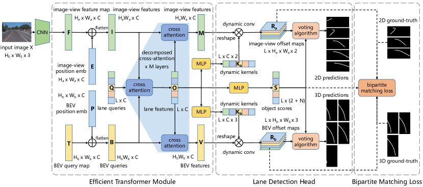
Figure 2: Overview of the proposed 3D lane detection framework. The framework includes a CNN backbone to extract an image-view feature map from the input image, an efficient transformer module to generate lane and BEV features simultaneously from the image-view features, a lane detection head to detect the 2D and 3D lane lines from the generated lane, image-view and BEV features, and a bipartite matching loss for model training. The dotted arrow parts are only engaged in training.

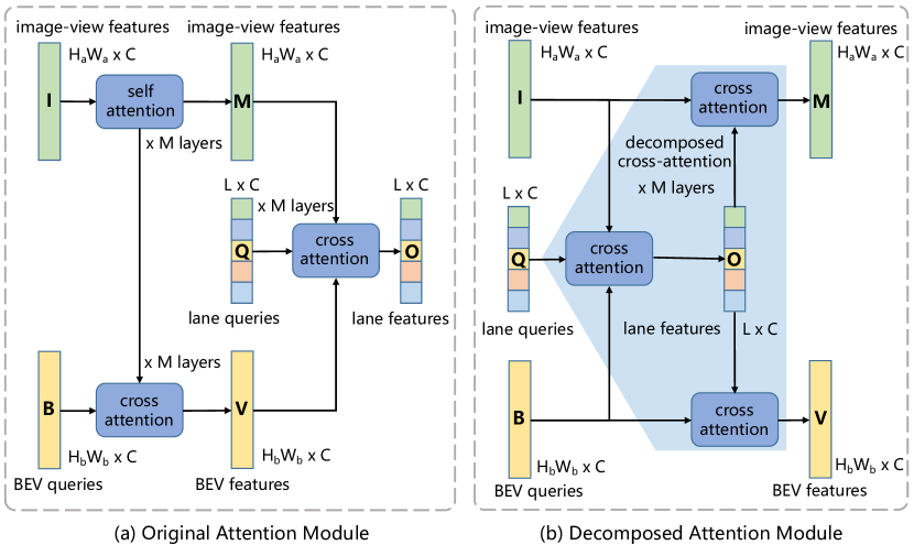
Figure 3: The comparison of learning lane and BEV representations between the original attention module and the decomposed attention module.

Figure 4: Visualization of attention maps between lane features O and image-view features M, and between O and BEV features V.

3.1 Overall Framework

The overall framework is shown in Figure 2. It starts with a CNN backbone to extract an image-view feature map from the input image. Then the efficient transformer module learns the lane and bird’s-eye view (BEV) features from the image-view features with a decomposed cross-attention mechanism. The image-view and BEV features are added with a position embeddings with their respective position encoders. Next, the lane detection head generates a set of dynamic kernels and object scores for each lane line using the lane features. These kernels are then used to convolve the image-view and BEV feature maps, producing image-view and BEV offset maps, respectively. The two sets of offset maps are processed with a voting algorithm to obtain the final 2D and 3D lane points, respectively. To train the model, a bipartite matching loss is calculated between the 2D/3D predictions and ground-truths. Thanks to the decomposed cross-attention mechanism, our framework achieves more accurate view transformation and lane detection while maintaining real-time efficiency.

3.2 Efficient Transformer Module

Here we describe how to learn the lane and BEV features simultaneously with the decomposed cross-attention mechanism. As shown in Figure 2, given an input image $\textbf{X}\in\mathbb{R}^{H_{0}\times W_{0}\times 3}$, we first adopt a CNN backbone to extract an image-view feature map $\textbf{F}\in\mathbb{R}^{H_{a}\times W_{a}\times C}$, where $H_{a}$, $W_{a}$ and $C$ are the height, width, and channels of F, respectively. The feature map F is added with a position embedding $\textbf{E}\in\mathbb{R}^{H_{a}\times W_{a}\times C}$ generated by a position encoder (described in Sec. 3.3), and then flattened into a sequence $\textbf{I}\in\mathbb{R}^{H_{a}W_{a}\times C}$. Then we initialize a BEV query map $\textbf{T}\in\mathbb{R}^{H_{b}\times W_{b}\times C}$ with learnable parameters, which is also added with a position embedding $\textbf{P}\in\mathbb{R}^{H_{b}\times W_{b}\times C}$ generated by another position encoder, and then flattened into a sequence $\textbf{B}\in\mathbb{R}^{H_{b}W_{b}\times C}$.

After obtaining the image-view features and the BEV queries, we initialize a set of lane queries $\textbf{Q}\in\mathbb{R}^{L\times C}$ with learnable parameters, representing $L$ different prototypes of lane lines. Then the lane features $\textbf{O}\in\mathbb{R}^{L\times C}$ are learned from the image-view features I and BEV queries B with a cross-attention. Let $\textbf{O}_{i}\in\mathbb{R}^{C}$ denote the $i$-th lane feature corresponds to the $i$-th lane query $\textbf{Q}_{i}$, $\textbf{O}_{i}$ can be obtained by

$$\textbf{Q}_{i}+\sum_{j=1}^{H_{a}W_{a}}f_{o}(\textbf{Q}_{i},\textbf{I}_{j})g_{o}(\textbf{I}_{j})+\sum_{k=1}^{H_{b}W_{b}}f_{o}(\textbf{Q}_{i},\textbf{B}_{k})g_{o}(\textbf{B}_{k}),$$ (1)

where $\textbf{I}_{j},\textbf{B}_{k}\in\mathbb{R}^{C}$ are the features at the $j$-th and $k$-th position of I and B, respectively; $g_{o}(\textbf{I}_{j})=\textbf{W}_{g}\textbf{I}_{j}$ is a linear transformation function where $\textbf{W}_{g}\in\mathbb{R}^{C\times C}$ is a learnable weight matrix; $f_{o}(\textbf{Q}_{i},\textbf{I}_{j})$ computes a pairwise similarity between $\textbf{Q}_{i}$ and $\textbf{I}_{j}$ as follows:

$$f_{o}(\textbf{Q}_{i},\textbf{I}_{j})=\frac{exp(\textbf{Q}_{i}^{\intercal}\textbf{W}_{\theta}^{\intercal}\textbf{W}_{\phi}\textbf{I}_{j})}{\sum_{j^{\prime}=1}^{H_{a}W_{a}}exp(\textbf{Q}_{i}^{\intercal}\textbf{W}_{\theta}^{\intercal}\textbf{W}_{\phi}\textbf{I}_{j^{\prime}})},$$ (2)

where $\textbf{W}_{\theta},\textbf{W}_{\phi}\in\mathbb{R}^{C\times C}$ are learnable weight matrices.

Then the BEV features V are constructed from the lane features O with a cross-attention as follows:

$$\textbf{V}_{i}=\textbf{B}_{i}+\sum_{j=1}^{L}f_{v}(\textbf{B}_{i},\textbf{O}_{j})g_{v}(\textbf{O}_{j}),$$ (3)

where $g_{v}(\cdot)$ and $f_{v}(\cdot,\cdot)$ have the same form as $g_{o}(\cdot)$ and $f_{o}(\cdot,\cdot)$ in Eq. (1), respectively, except for their learnable weight matrices. In this way, the original cross-attention between the BEV features V and the image-view features I shown in Figure 3 is decomposed into the one between the image-view features I and the lane features O, and the one between the lane features O and the BEV features V.

Compared to the original one, the decomposed cross-attention provides three benefits. Firstly, it enables better view transformation by supervising the decomposed cross-attentions with 2D and 3D ground-truth lane lines. The 2D and 3D lane predictions are obtained by applying the lane features O to the image-view features I and the BEV features V, respectively. Secondly, it improves the accuracy of 3D lane detection by enabling the dynamic adjustment between the lane features O and the BEV features V through cross-attention. Thirdly, it significantly reduces the computation amount and enables real-time efficiency.

Similarly, the image-view features I are updated with the object features O with a cross-attention as follows:

$$\textbf{M}_{i}=\textbf{I}_{i}+\sum_{j=1}^{L}f_{m}(\textbf{I}_{i},\textbf{O}_{j})g_{m}(\textbf{O}_{j}),$$ (4)

where M is the updated image-view features, $g_{m}(\cdot)$ and $f_{m}(\cdot,\cdot)$ has the same form as $g_{o}(\cdot)$ and $f_{o}(\cdot,\cdot)$ in Eq. (1), respectively, except for their learnable weight matrices. In this way, the original self-attention within the image-view features I shown in Figure 3 is decomposed into the back-and-forth cross-attention between the image-view features I and the lane features O.

Compared to the original one, the decomposed self-attention improves the accuracy of 2D lane detection by enabling the dynamic adjustment between the lane features O and the image-view features I through cross-attention. Moreover, since the image-view features M and the BEV features V are both constructed from the object features O, they can better align with each other.

3.3 Position Embedding

Here we describe how to generate the position embeddings for transfomer inputs. For the image-view position embedding $\textbf{E}\in\mathbb{R}^{H_{a}\times W_{a}\times C}$, we first constructs a 3D coordinate grid $\textbf{G}\in\mathbb{R}^{H_{a}\times W_{a}\times D\times 4}$ in camera space, where $D$ is the number of discretized depth bins. Each point in G can be represented as $p_{j}=(u_{j}\times d_{j},v_{j}\times d_{j},d_{j},1)^{\intercal}$, where $(u_{j},v_{j})$ is the corresponding pixel coordinate in the image-view feature map F, $d_{j}$ is the corresponding depth value.

Then the grid G is transformed into a grid $\textbf{G}^{\prime}\in\mathbb{R}^{H_{a}\times W_{a}\times D\times 4}$ in 3D space as follows:

$$p_{j}^{\prime}=K^{-1}p_{j},$$ (5)

where $p_{j}^{\prime}$ is the point in $\textbf{G}^{\prime}$ corresponding to the point $p_{j}$ in G, $K\in\mathbb{R}^{4\times 4}$ is a projection matrix from the 3D space to the camera space. Then we predict the depth distributions $\textbf{D}\in\mathbb{R}^{H_{a}\times W_{a}\times D}$ from F, indicating the probability of each pixel belonging to each depth bin. Then the position embedding E is obtained as follows:

$$\textbf{E}_{uv}=\left[\sum_{d=1}^{D}\textbf{D}_{uvd}(\textbf{G}^{\prime}_{uvd}\textbf{W}_{1}+\textbf{b}_{1})\right]\textbf{W}_{2}+\textbf{b}_{2},$$ (6)

where $\textbf{E}_{uv}\in\mathbb{R}^{C}$ is the pixel embedding at $u$-th row and $v$-th column of F; $\textbf{W}_{1}\in\mathbb{R}^{4\times C/4}$, $\textbf{b}_{1}\in\mathbb{R}^{C/4}$, $\textbf{W}_{2}\in\mathbb{R}^{C/4\times C}$ and $\textbf{b}_{2}\in\mathbb{R}^{C}$ are learnable weights.

For the BEV position embedding $\textbf{P}\in\mathbb{R}^{H_{b}\times W_{b}\times C}$, we first constructs a 3D coordinate grid $\textbf{H}\in\mathbb{R}^{H_{b}\times W_{b}\times Z\times 4}$ in 3D space, where $Z$ is the number of discretized height bins. Each point in H can be represented as $p_{i}=(x_{i}\times s_{x}+r_{x}^{0},y_{i}\times s_{y}+r_{y}^{0},z_{i},1)^{\intercal}$, where $(x_{i},y_{i})$ is the corresponding pixel coordinate in the BEV query map T; $z_{i}$ is the corresponding height value; $s_{x}=(r_{x}^{1}-r_{x}^{0})/W_{b}$ and $(r_{x}^{0},r_{x}^{1})$ are the scale factor and range for the $x$ direction in 3D space, respectively (similar for $s_{y}$ and $r_{y}$).

Then we predict the height distributions $\textbf{Z}\in\mathbb{R}^{H_{b}\times W_{b}\times Z}$ from T, indicating the probability of each pixel belonging to each height bin. Then the position embedding P is obtained as follows:

$$\textbf{P}_{xy}=\left[\sum_{z=1}^{Z}\textbf{Z}_{xyz}(\textbf{H}_{xyz}\textbf{W}_{1}+\textbf{b}_{1})\right]\textbf{W}_{2}+\textbf{b}_{2},$$ (7)

where $\textbf{P}_{xy}\in\mathbb{R}^{C}$ is the pixel embedding at $x$-th row and $y$-th column of T; $\textbf{W}_{1}$, $\textbf{b}_{1}$, $\textbf{W}_{2}$ and $\textbf{b}_{2}$ are the same as those in Eq. (6).

Input: $\textbf{R}_{b}$: BEV offset maps, S: object scores,   $r_{x}$, $r_{y}$: $x$ and $y$ ranges in 3D space,     $t$: object threshold, $w$: lane width threshold

1 Initialize a vote count matrix $\textbf{U}_{b}\in\mathbb{R}^{L\times H_{b}\times W_{b}}$

2 Initialize a BEV lane line set $\textbf{Y}_{b}=\emptyset$

3 for $i=0$ to $L-1$ do

4       for $j=0$ to $H_{b}-1$ do

5             for $k=0$ to $W_{b}-1$ do

6                   $x,y\leftarrow\left[k+\textbf{R}_{b}^{ijk0}\right],\left[j+\textbf{R}_{b}^{ijk1}\right]$

7                   $s\leftarrow exp(-(\frac{(\textbf{R}_{b}^{ijk0})^{2}+(\textbf{R}_{b}^{ijk1})^{2})}{2w^{2}})$

8                   $\textbf{U}_{b}^{iyx}\leftarrow\textbf{U}_{b}^{iyx}+s$

9                  

10            

11      Initialize a BEV lane point set $\textbf{L}_{b}=\emptyset$

12       for $j=0$ to $H_{b}-1$ do

13             for $k=0$ to $W_{b}-1$ do

14                   if $\textbf{U}_{b}^{ijk}\geq w$ then

15                         $x\leftarrow k\times(r_{x}^{1}-r_{x}^{0})/W_{b}+r_{x}^{0}$

16                         $y\leftarrow j\times(r_{y}^{1}-r_{y}^{0})/H_{b}+r_{y}^{0}$

17                         $z\leftarrow\textbf{R}_{b}^{ijk2}$

18                         $\textbf{L}_{b}\leftarrow\textbf{L}_{b}\cup\{(x,y,z)\}$

19                        

20                  

21            

22      if $\textbf{S}_{i1}\geq t$ then

23             $\textbf{Y}_{b}\leftarrow\textbf{Y}_{b}\cup\{\textbf{L}_{b}\}$

24            

25      

Output: the BEV lane line set $\textbf{Y}_{b}$.

Algorithm 1 The voting algorithm.

3.4 Lane Detection Head

Here we describe the lane detection head. We first apply two multi-layer perceptrons (MLPs) to the lane features O to generate two sets of dynamic kernels $\textbf{K}_{a}\in\mathbb{R}^{L\times C\times 2}$ and $\textbf{K}_{b}\in\mathbb{R}^{L\times C\times 3}$, respectively. Then we apply $\textbf{K}_{a}$ and $\textbf{K}_{b}$ to convolve the image-view features M and the BEV features V, to obtain the image-view offset map $\textbf{R}_{a}\in\mathbb{R}^{L\times H_{a}\times W_{a}\times 2}$ and the BEV offset map $\textbf{R}_{b}\in\mathbb{R}^{L\times H_{b}\times W_{b}\times 3}$, respectively. $\textbf{R}_{a}$ predicts the horizontal and vertical offsets of each pixel to its nearest lane point in image view; $\textbf{R}_{b}$ predicts the offsets in $x$ and $y$ directions of each pixel to its nearest lane point in BEV, along with the real height of the lane point.

Then we apply another MLP to the lane features O to generate the object scores $\textbf{S}\in\mathbb{R}^{L\times(2+N)}$, including the probabilities of background, foreground, and $N$ lane classes. Then the image-view offset maps $\textbf{R}_{a}$ and the BEV offset maps $\textbf{R}_{b}$ are processed with a voting algorithm to obtain the 2D and 3D lane points, respectively. The process of $\textbf{R}_{b}$ is shown in Algorithm 1 (similar for $\textbf{R}_{a}$, except for the removal of $z$ and $r$). The voting algorithm casts votes for the predicted lane points of all pixels, and then selects those with votes exceeding a lane width threshold $w$ to form a predicted lane line. Finally, only the predicted lane lines with a foreground probability exceeding an object threshold $t$ are retained as output.

3.5 Bipartite Matching Loss

Here we introduce the design of loss functions. First, we need to compute a pair-wise matching cost $L_{match}(\textbf{Y}_{i},\textbf{Y}_{j}^{*})$ between $L$ predicted lane lines $\textbf{Y}=\{\textbf{Y}_{i}\}_{i=1}^{L}$ and $M$ ground-truth lane lines $\textbf{Y}^{*}=\{\textbf{Y}_{i}^{*}\}_{i=1}^{L}$, where each $\textbf{Y}_{i}$ contains object scores S, image-view offset maps $\textbf{R}_{a}$ and BEV offset maps $\textbf{R}_{b}$ (same for $\textbf{Y}_{i}^{*}$). The matching cost includes an object cost, a classification cost and an offset map cost. The object cost is defined as follows:

$$L_{obj}(\textbf{Y}_{i},\textbf{Y}_{j}^{*})=-log(\textbf{S}_{i1}),$$ (8)

where $\textbf{S}_{i1}$ is the predicted foreground probability of the $i$-th predicted lane line. The classification cost is defined as follows:

$$L_{cls}(\textbf{Y}_{i},\textbf{Y}_{j}^{*})=-\sum_{k=0}^{N-1}\textbf{S}_{j(k+2)}^{*}\cdot log(\textbf{S}_{i(k+2)}),$$ (9)

where $\textbf{S}_{i(k+2)}$ is the predicted probability of the $k$-th class of the $i$-th prediction, $\textbf{S}_{j(k+2)}^{*}$ is the corresponding label of the $j$-th ground-truth, $N$ is the number of classes. The offset map cost is defined as follows:

$$L_{off}(\textbf{Y}_{i},\textbf{Y}_{j}^{*})= \frac{1}{H_{a}W_{a}}\sum_{m=0}^{H_{a}-1}\sum_{n=0}^{W_{a}-1}\|\textbf{R}_{a}^{imn}-(\textbf{R}_{a}^{jmn})^{*}\|_{1}$$ (10)

$$+ \frac{1}{H_{b}W_{b}}\sum_{m=0}^{H_{b}-1}\sum_{n=0}^{W_{b}-1}\|\textbf{R}_{b}^{imn}-(\textbf{R}_{b}^{jmn})^{*}\|_{1},$$

where $\textbf{R}_{a}^{i}\in\mathbb{R}^{H_{a}\times W_{a}\times 2}$ and $\textbf{R}_{b}^{i}\in\mathbb{R}^{H_{b}\times W_{b}\times 3}$ are the predicted image-view and BEV offset maps of the $i$-th prediction, $(\textbf{R}_{b}^{j})^{*}$ and $(\textbf{R}_{a}^{j})^{*}$ are the corresponding labels of the $j$-th ground-truth. The final pair-wise matching cost is defined as follows:

$$L_{match}(\textbf{Y}_{i},\textbf{Y}_{j}^{*}) =\lambda_{obj}L_{obj}(\textbf{Y}_{i},\textbf{Y}_{j}^{*})+\lambda_{cls}L_{cls}(\textbf{Y}_{i},\textbf{Y}_{j}^{*})$$ (11)

$$+\lambda_{off}L_{off}(\textbf{Y}_{i},\textbf{Y}_{j}^{*}),$$

where $\lambda_{obj}$, $\lambda_{cls}$ and $\lambda_{off}$ are the balance weights for $L_{obj}$, $L_{cls}$ and $L_{off}$, respectively. Then we find an optimal injective function $z:\{\textbf{Y}_{i}\}_{i=1}^{L}\rightarrow\{\textbf{Y}_{j}^{*}\}_{j=1}^{M}$, where $z(j)$ is the index of the prediction assigned to the $j$-th ground-truth, by minimizing the matching cost as follows:

$$\underset{z}{{\arg\min}\,\hat{z}}=\sum_{j=1}^{N}L_{match}(\textbf{Y}_{z(j)},\textbf{Y}_{j}^{*}).$$ (12)

This objective function can be solved by the Hungarian algorithm [16]. After obtaining the injective mapping $z$, we can compute the final loss function as follows:

$$loss =\frac{1}{M}\sum_{j=1}^{M}\big{[}\lambda_{obj}L_{obj}(\textbf{Y}_{z(j)},\textbf{Y}_{j}^{*})+\lambda_{cls}L_{cls}(\textbf{Y}_{z(j)},\textbf{Y}_{j}^{*})$$ (13)

$$+ \lambda_{off}L_{off}(\textbf{Y}_{z(j)},\textbf{Y}_{j}^{*})\big{]}+\frac{1}{L-M}\sum_{i\notin\textbf{C}}\lambda_{obj}L_{obj}(\textbf{Y}_{i},\phi),$$

where $\textbf{C}=\{z(j)\}_{j=1}^{M}$ is the index set of the predictions matched to the ground-truths, $L_{obj}(\textbf{Y}_{i},\phi)=-log(\textbf{S}_{i0})$, where $\textbf{S}_{i0}$ is the predicted background probability of the $i$-th prediction.

4 Experiment

Method	Backbone	F1(%)	Cate Acc.(%)	X err. near (m)	X err. far (m)	Z err. near (m)	Z err. far (m)
3D-LaneNet [9]	VGG-16	44.1	-	0.479	0.572	0.367	0.443
GenLaneNet [10]	ERFNet	32.3	-	0.591	0.684	0.411	0.521
PersFormer [4]	EfficientNet	50.5	92.3	0.485	0.553	0.364	0.431
CurveFormer [1]	EfficientNet	50.5	-	0.340	0.772	0.207	0.651
Anchor3DLane [12]	ResNet-18	54.3	90.7	0.275	0.310	0.105	0.135
BEV-LaneDet [32]	ResNet-18	57.8	-	0.318	0.705	0.245	0.629
BEV-LaneDet [32]	ResNet-34	58.4	-	0.309	0.659	0.244	0.631
Ours	ResNet-18	60.7	89.2	0.287	0.358	0.112	0.143
Ours	ResNet-34	62.8	91.2	0.254	0.322	0.105	0.135
Ours	EfficientNet	63.8	91.5	0.245	0.304	0.104	0.129

Table 1: Comparison with state-of-the-art methods on OpenLane validation set. We report the F-score, category accuracy, and regression errors in x and z directions of the models.

Method	Backbone	All	Up & Down	Curve	Extreme Weather	Night	Intersection	Merge & Split
3D-LaneNet [9]	VGG-16	44.1	40.8	46.5	47.5	41.5	32.1	41.7
GenLaneNet [10]	ERFNet	32.3	25.4	33.5	28.1	18.7	21.4	31.0
PersFormer [4]	EfficientNet	50.5	42.4	55.6	48.6	46.6	40.0	50.7
CurveFormer [1]	EfficientNet	50.5	45.2	56.6	49.7	49.1	42.9	45.4
Anchor3DLane [12]	ResNet-18	54.3	47.2	58.0	52.7	48.7	45.8	51.7
BEV-LaneDet [32]	ResNet-34	58.4	48.7	63.1	53.4	53.4	50.3	53.7
Ours	ResNet-18	60.7	56.9	69.4	53.8	55.3	53.8	60.1
Ours	ResNet-34	62.8	56.9	71.0	54.3	57.9	55.9	63.1
Ours	EfficientNet	63.8	57.6	73.2	57.3	59.7	57.0	64.9

Table 2: Comparison with state-of-the-art methods on OpenLane validation set. We report the F-score for the whole validation set and under different scenarios, including curve, intersection, night, extreme weather, merge and split, and up and down.

Method	Backbone	F1(%)	Prec.(%)	Rec.(%)	CD Err.(m)
3D-LaneNet [9]	VGG-16	44.73	61.46	35.16	0.127
GenLaneNet [10]	ERFNet	45.59	63.95	35.42	0.121
SALAD [36]	Segformer	64.07	75.90	55.42	0.098
PersFormer [4]	EfficientNet	74.33	80.30	69.18	0.074
Anchor3DLane [12]	ResNet-18	74.87	80.85	69.71	0.060
Ours	ResNet-18	79.67	82.66	76.89	0.057
Ours	ResNet-34	80.49	84.67	76.70	0.057
Ours	EfficientNet	80.84	84.50	77.48	0.056

Table 3: Comparison with state-of-the-art methods on ONCE-3DLanes test set. We report the F-score, precision, recall and chamfer distance (CD) error of the models.

4.1 Datasets

We conduct experiments on two 3D lane detection benchmarks: OpenLane [4] and ONCE-3DLanes [36]. OpenLane contains $160K$ and $40K$ images for training and validation sets, respectively. The validation set consists of six different scenarios, including curve, intersection, night, extreme weather, merge and split, and up and down. It annotates $14$ lane categories, including road edges, double yellow solid lanes, and so on. ONCE-3DLanes contains $200$K, $3$K, and $8$K images for training, validation, and testing, respectively, covering different time periods including morning, noon, afternoon and night, various weather conditions including sunny, cloudy and rainy days, as well as a variety of regions including downtown, suburbs, highway, bridges and tunnels.

4.2 Evaluation Metrics

Following [4], we adopt the F-score for regression and the accuracy of matched lanes for classification. We match predictions to ground truth using edit distance, where a predicted lane is only considered a true positive if 75% of its y-positions have a point-wise distance less than the maximum allowed distance of $1.5$ meters. For ONCE-3DLanes, following [36], we adopt a two-stage evaluation metric to measure the similarity between predicted and ground-truth lanes. We first use the traditional IoU method to match lanes in the top-view. If the IoU is greater than a threshold ($0.3$), we use a unilateral Chamfer Distance to calculate the curves matching error. If the chamfer distance is less than a threshold ($0.3$m), we consider the predicted lane a true positive. At last, we use precision, recall, and F-score as metrics.

4.3 Implementation Details

We adopt ResNet-18, ResNet-34 [11], EfficientNet(-B7) [30] with the pretrained weights from ImageNet [7] as the CNN backbones. The input images are augmented with random horizontal flipping and random rotation, and resized to $368\times 480$. The spatial resolution of the BEV feature map is $50\times 32$, representing a BEV space with the range of $\left[-10,10\right]\times\left[3,103\right]$ meters along $x$ and $y$ directions, respectively. The BEV offset map is resized to $400\times 256$ for final prediction. Optimization is done by AdamW [23] with betas of $0.9$ and $0.999$, and weight decay of $1e^{-4}$. The batch size is set to $16$. We train the model for $50$ epochs. The base learning rate is initialized at $1e^{-4}$ and decayed to $1e^{-5}$ after $40$ epochs. The learning rate for the backbone is set to $0.1$ times of the base learning rate. The lane query number $L$ is set to $80$. The weights $\lambda_{obj}$, $\lambda_{cls}$, and $\lambda_{off}$ are set to $5$, $5$, and $1$, respectively, to balance different losses, i.e., bring them to the same scale. The object threshold $t$ is set to $0.7$. The lane width threshold $w$ is set to $16$.

4.4 Results

Performance on OpenLane Dataset.

The comparison results on OpenLane are shown in Table 1. Using ResNet-18 as backbone, our method achieves a F-score of $60.7$, which is $10.2$, $6.4$ and $2.9$ points higher than that of PersFormer, Anchor3DLane and BEV-LaneDet, respectively. Our method also achieves the lowest prediction errors along the x, y and z directions. As shown in Table 2, our method achieves the best performance in all of the six scenarios, demonstrating the robustness of our method. For example, for the “Up & Down”, “Curve”, “Intersection” and “Merge & Split” scenarios, using ResNet-34 as backbone, the F-scores of our method are $8.2$, $7.9$, $5.6$ and $9.4$ points higher than those of BEV-LaneDet, respectively. In Figure 5, we show qualitative comparison results on OpenLane, including upill, downhill, curved and forked scenarios. The comparison results demonstrate that our method can cope with the lane lines on uneven roads and those with complex topologies very well. This is because simultaneously learning lane and BEV features under supervision allows them to adjust with each other to generate more accurate results than the separate two-stage pipeline.

Performance on ONCE-3DLanes Dataset.

The comparison results on ONCE-3DLanes is shown in Table 3. Using ResNet-18 as backbone, our method achieves a F-score of $79.67$, which is $15.60$, $5.34$ and $4.80$ points higher than that of SALAD, PersFormer and Anchor3DLane, respectively. Our method also achieves the lowest CD errors, demonstrating the good accuracy of the proposed method.

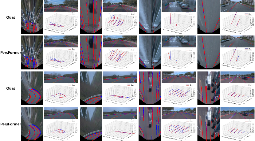
Figure 5: Visualization results on OpenLane. We choose PersFormer [4] as our comparison method. We visualize the results under different scenarios, where the first two rows include uphill and downhill cases, and the last two rows include curved and forked lane lines. The blue lane lines are ground-truths and the red lane lines are predictions.

4.5 Ablation Studies

Exp.	IPM-based Attention	Original Attention	Decomposed Attention	OpenLane			ONCE-3DLanes			FPS
				F1(%)	Prec.(%)	Rec.(%)	F1(%)	Prec.(%)	Rec.(%)
1	✔	✘	✘	58.6	63.6	54.3	77.5	81.3	74.1	25
2	✘	✔	✘	59.5	63.4	56.2	78.2	81.5	75.2	17
3	✘	✘	✔	62.8	67.8	58.5	80.5	84.7	76.7	45

Table 4: The comparison results between different attention mechanisms on OpenLane and ONCE-3DLanes datasets. The backbone we use is ResNet-34.

Num of lane queries	OpenLane			ONCE-3DLanes
	F1	Prec.	Rec.	F1	Prec.	Rec.
20	59.4	64.4	55.2	78.1	82.5	74.2
40	61.3	66.2	57.1	79.4	83.8	75.4
80	62.8	67.8	58.5	80.5	84.7	76.7
160	63.7	68.7	59.4	81.1	85.4	77.2

Table 5: Comparison of the results with different number of lane queries on OpenLane and ONCE-3DLanes datasets. The backbone we use is ResNet-34.

Influence of decomposed attention.

We compare the results of the proposed decomposed attention (Fig. 3 (b)), the original attention (Fig. 3 (a)) and IPM-based attention. The IPM-based attention is used in PersFormer [4] for view transformation, where the reference points of the deformable transformer are computed with IPM. As shown in Table 4, the performance of the original attention is slightly better than that of the IPM-based attention, and the F1 scores of the decomposed attention are $3.3$ and $2.3$ points higher than those of the original attention on OpenLane and ONCE-3DLanes, respectively. This is because the decomposed attention allows for more accurate view transformation by supervising the cross-attention between the image-view and lane features, as well as the cross-attention between the lane and BEV features, using 2D and 3D ground-truths respectively. Additionally, it improves the accuracy of 3D lane detection by enabling dynamic adjustments between lane and BEV features through cross-attention. The speed of the decomposed attention is $2.6$ times that of the original attention, demonstrating the efficiency of the proposed decomposed attention mechanism.

Number of lane queries.

Here we investigate the influence of different number of lane queries. As shown in Table 5, when we increase the number of lane queries from $20$ to $80$, the performance is improved. This demonstrates that increasing the number of lane queries is beneficial to the transformation between image-view and BEV features. When we further increase the number of lane queries from $80$ to $160$, the performance only increases slightly, which is because an excessive number of lane queries can cause redundancy.

5 Conclusion

In this paper, we propose an efficient transformer for 3D lane detection, utilizing a decomposed attention mechanism to simultaneously learn lane and BEV representations. The mechanism decomposes the cross-attention between image-view and BEV features into the one between image-view and lane features, and the one between lane and BEV features, both of which are supervised with ground-truth lane lines. This allows for a more accurate view transformation than IPM-based methods, and a more accurate lane detection than the traditional two-stage pipeline.

References

- [1] Yifeng Bai, Zhirong Chen, Zhangjie Fu, Lang Peng, Pengpeng Liang, and Erkang Cheng. Curveformer: 3d lane detection by curve propagation with curve queries and attention. arXiv preprint arXiv:2209.07989, 2022.
- [2] Christopher TH Baker. The numerical treatment of integral equations. 1977.
- [3] Iz Beltagy, Matthew E Peters, and Arman Cohan. Longformer: The long-document transformer. arXiv preprint arXiv:2004.05150, 2020.
- [4] Li Chen, Chonghao Sima, Yang Li, Zehan Zheng, Jiajie Xu, Xiangwei Geng, Hongyang Li, Conghui He, Jianping Shi, Yu Qiao, et al. Persformer: 3d lane detection via perspective transformer and the openlane benchmark. arXiv preprint arXiv:2203.11089, 2022.
- [5] Ziye Chen, Mingming Gong, Lingjuan Ge, and Bo Du. Compressed self-attention for deep metric learning with low-rank approximation. In IJCAI, pages 2058–2064, 2020.
- [6] Zhenpeng Chen, Qianfei Liu, and Chenfan Lian. Pointlanenet: Efficient end-to-end cnns for accurate real-time lane detection. In 2019 IEEE intelligent vehicles symposium (IV), pages 2563–2568. IEEE, 2019.
- [7] Jia Deng, Wei Dong, Richard Socher, Li-Jia Li, Kai Li, and Li Fei-Fei. Imagenet: A large-scale hierarchical image database. In 2009 IEEE conference on computer vision and pattern recognition, pages 248–255. Ieee, 2009.
- [8] Netalee Efrat, Max Bluvstein, Shaul Oron, Dan Levi, Noa Garnett, and Bat El Shlomo. 3d-lanenet+: Anchor free lane detection using a semi-local representation. arXiv preprint arXiv:2011.01535, 2020.
- [9] Noa Garnett, Rafi Cohen, Tomer Pe’er, Roee Lahav, and Dan Levi. 3d-lanenet: end-to-end 3d multiple lane detection. In Proceedings of the IEEE/CVF International Conference on Computer Vision, pages 2921–2930, 2019.
- [10] Yuliang Guo, Guang Chen, Peitao Zhao, Weide Zhang, Jinghao Miao, Jingao Wang, and Tae Eun Choe. Gen-lanenet: A generalized and scalable approach for 3d lane detection. In European Conference on Computer Vision, pages 666–681. Springer, 2020.
- [11] Kaiming He, Xiangyu Zhang, Shaoqing Ren, and Jian Sun. Deep residual learning for image recognition. In Proceedings of the IEEE conference on computer vision and pattern recognition, pages 770–778, 2016.
- [12] Shaofei Huang, Zhenwei Shen, Zehao Huang, Zihan Ding, Jiao Dai, Jizhong Han, Naiyan Wang, and Si Liu. Anchor3dlane: Learning to regress 3d anchors for monocular 3d lane detection. arXiv preprint arXiv:2301.02371, 2023.
- [13] Zilong Huang, Xinggang Wang, Lichao Huang, Chang Huang, Yunchao Wei, and Wenyu Liu. Ccnet: Criss-cross attention for semantic segmentation. In Proceedings of the IEEE/CVF international conference on computer vision, pages 603–612, 2019.
- [14] Max Jaderberg, Karen Simonyan, Andrew Zisserman, et al. Spatial transformer networks. Advances in neural information processing systems, 28, 2015.
- [15] Yeongmin Ko, Younkwan Lee, Shoaib Azam, Farzeen Munir, Moongu Jeon, and Witold Pedrycz. Key points estimation and point instance segmentation approach for lane detection. IEEE Transactions on Intelligent Transportation Systems, 2021.
- [16] Harold W Kuhn. The hungarian method for the assignment problem. Naval research logistics quarterly, 2(1-2):83–97, 1955.
- [17] Chenguang Li, Jia Shi, Ya Wang, and Guangliang Cheng. Reconstruct from top view: A 3d lane detection approach based on geometry structure prior. In Proceedings of the IEEE/CVF Conference on Computer Vision and Pattern Recognition, pages 4370–4379, 2022.
- [18] Qi Li, Yue Wang, Yilun Wang, and Hang Zhao. Hdmapnet: An online hd map construction and evaluation framework. arXiv e-prints, pages arXiv–2107, 2021.
- [19] Qi Li, Yue Wang, Yilun Wang, and Hang Zhao. Hdmapnet: An online hd map construction and evaluation framework. In 2022 International Conference on Robotics and Automation (ICRA), pages 4628–4634. IEEE, 2022.
- [20] Lizhe Liu, Xiaohao Chen, Siyu Zhu, and Ping Tan. Condlanenet: a top-to-down lane detection framework based on conditional convolution. In Proceedings of the IEEE/CVF International Conference on Computer Vision, pages 3773–3782, 2021.
- [21] Ruijin Liu, Zejian Yuan, Tie Liu, and Zhiliang Xiong. End-to-end lane shape prediction with transformers. In Proceedings of the IEEE/CVF winter conference on applications of computer vision, pages 3694–3702, 2021.
- [22] Ze Liu, Yutong Lin, Yue Cao, Han Hu, Yixuan Wei, Zheng Zhang, Stephen Lin, and Baining Guo. Swin transformer: Hierarchical vision transformer using shifted windows. In Proceedings of the IEEE/CVF international conference on computer vision, pages 10012–10022, 2021.
- [23] Ilya Loshchilov and Frank Hutter. Decoupled weight decay regularization. arXiv preprint arXiv:1711.05101, 2017.
- [24] Annika Meyer, N Ole Salscheider, Piotr F Orzechowski, and Christoph Stiller. Deep semantic lane segmentation for mapless driving. In 2018 IEEE/RSJ International Conference on Intelligent Robots and Systems (IROS), pages 869–875. IEEE, 2018.
- [25] Davy Neven, Bert De Brabandere, Stamatios Georgoulis, Marc Proesmans, and Luc Van Gool. Towards end-to-end lane detection: an instance segmentation approach. In 2018 IEEE intelligent vehicles symposium (IV), pages 286–291. IEEE, 2018.
- [26] Zhan Qu, Huan Jin, Yang Zhou, Zhen Yang, and Wei Zhang. Focus on local: Detecting lane marker from bottom up via key point. In Proceedings of the IEEE/CVF Conference on Computer Vision and Pattern Recognition, pages 14122–14130, 2021.
- [27] Jinming Su, Chao Chen, Ke Zhang, Junfeng Luo, Xiaoming Wei, and Xiaolin Wei. Structure guided lane detection. arXiv preprint arXiv:2105.05403, 2021.
- [28] Lucas Tabelini, Rodrigo Berriel, Thiago M Paixao, Claudine Badue, Alberto F De Souza, and Thiago Oliveira-Santos. Keep your eyes on the lane: Real-time attention-guided lane detection. In Proceedings of the IEEE/CVF conference on computer vision and pattern recognition, pages 294–302, 2021.
- [29] Lucas Tabelini, Rodrigo Berriel, Thiago M Paixao, Claudine Badue, Alberto F De Souza, and Thiago Oliveira-Santos. Polylanenet: Lane estimation via deep polynomial regression. In 2020 25th International Conference on Pattern Recognition (ICPR), pages 6150–6156. IEEE, 2021.
- [30] Mingxing Tan and Quoc Le. Efficientnet: Rethinking model scaling for convolutional neural networks. In International conference on machine learning, pages 6105–6114. PMLR, 2019.
- [31] Jun Wang, Tao Mei, Bin Kong, and Hu Wei. An approach of lane detection based on inverse perspective mapping. In 17th International IEEE Conference on Intelligent Transportation Systems (ITSC), pages 35–38. IEEE, 2014.
- [32] Ruihao Wang, Jian Qin, Kaiying Li, and Dong Cao. Bev lane det: Fast lane detection on bev ground. arXiv preprint arXiv:2210.06006, 2022.
- [33] Sinong Wang, Belinda Z Li, Madian Khabsa, Han Fang, and Hao Ma. Linformer: Self-attention with linear complexity. arXiv preprint arXiv:2006.04768, 2020.
- [34] Yingming Wang, Xiangyu Zhang, Tong Yang, and Jian Sun. Anchor detr: Query design for transformer-based object detection. arXiv preprint arXiv:2109.07107, 3(6), 2021.
- [35] Yunyang Xiong, Zhanpeng Zeng, Rudrasis Chakraborty, Mingxing Tan, Glenn Fung, Yin Li, and Vikas Singh. Nyströmformer: A nyström-based algorithm for approximating self-attention. In Proceedings of the AAAI Conference on Artificial Intelligence, volume 35, pages 14138–14148, 2021.
- [36] Fan Yan, Ming Nie, Xinyue Cai, Jianhua Han, Hang Xu, Zhen Yang, Chaoqiang Ye, Yanwei Fu, Michael Bi Mi, and Li Zhang. Once-3dlanes: Building monocular 3d lane detection. In Proceedings of the IEEE/CVF Conference on Computer Vision and Pattern Recognition, pages 17143–17152, 2022.
- [37] Tu Zheng, Yifei Huang, Yang Liu, Wenjian Tang, Zheng Yang, Deng Cai, and Xiaofei He. Clrnet: Cross layer refinement network for lane detection. In Proceedings of the IEEE/CVF Conference on Computer Vision and Pattern Recognition, pages 898–907, 2022.
- [38] Xizhou Zhu, Weijie Su, Lewei Lu, Bin Li, Xiaogang Wang, and Jifeng Dai. Deformable detr: Deformable transformers for end-to-end object detection. arXiv preprint arXiv:2010.04159, 2020.