In-Context Learning through the Bayesian Prism

Abstract

In-context learning is one of the surprising and useful features of large language models. How it works is an active area of research. Recently, stylized meta-learning-like setups have been devised that train these models on a sequence of input-output pairs $(x,f(x))$ from a function class using the language modeling loss and observe generalization to unseen functions from the same class. One of the main discoveries in this line of research has been that for several problems such as linear regression, trained transformers learn algorithms for learning functions in context. However, the inductive biases of these models resulting in this behavior are not clearly understood. A model with unlimited training data and compute is a Bayesian predictor: it learns the pretraining distribution. It has been shown that high-capacity transformers mimic the Bayesian predictor for linear regression. In this paper, we show empirical evidence of transformers exhibiting the behavior of this ideal learner across different linear and non-linear function classes. We also extend the previous setups to work in the multitask setting and verify that transformers can do in-context learning in this setup as well and the Bayesian perspective sheds light on this setting also. Finally, via the example of learning Fourier series, we study the inductive bias for in-context learning. We find that in-context learning may or may not have simplicity bias depending on the pretraining data distribution.

1 Introduction

In-context learning (ICL) is one of the ingredients behind the astounding performance of large language models (LLMs) Brown et al. (2020); Workshop (2023); Touvron et al. (2023). Unlike traditional learning, ICL is the ability to learn new functions $f$ without weight updates during inference from input-output examples $(x,f(x))$; in other words, learning happens in context. For instance, given prompt up -> down, low -> high, small -> a pretrained LLM will likely produce output big. It infers that the function in the two examples is the antonym of the input and applies it on the new input. This behavior extends to more sophisticated and novel functions unlikely to have been seen during training and has been the subject of intense study, e.g. Min et al. (2022b); Webson and Pavlick (2022); Min et al. (2022a); Liu et al. (2023); Dong et al. (2023). Apart from its applications in NLP, more broadly ICL can also be viewed as providing a method for meta-learning Schmidhuber (1987); Thrun and Pratt (2012); Hospedales et al. (2022) where the model learns to learn a class of functions.

Theoretical understanding of ICL is an active area of research. Since the real-world datasets used for LLM training are difficult to model theoretically and are very large, ICL has also been studied in stylized setups Xie et al. (2022); Chan et al. (2022b); Garg et al. (2022); Wang et al. (2023); Hahn and Goyal (2023). These setups study different facets of ICL. In this paper, we focus on the framework of Garg et al. (2022) which is closely related to meta-learning. Unlike in NLP where training is done on documents for next-token prediction task, here the training and test data look similar in the sense that the training data consists of input of the form $((\bm{\mathit{x}}_{1},f(\bm{\mathit{x}}_{1})),\ldots,(\bm{\mathit{x}}_{k},f(\bm{\mathit{x}}_{k})),\bm{\mathit{x}}_{k+1})$ and output is $f(\bm{\mathit{x}}_{k+1})$, where $\bm{\mathit{x}}_{i}\in\mathbb{R}^{d}$ and are chosen i.i.d. from a distribution and $f:\mathbb{R}^{d}\to\mathbb{R}$ is a function from a family of functions, for example, linear functions or shallow neural networks. We call this setup including an extension we introduce in this paper MICL ; cf. Min et al. (2022a). A striking discovery in Garg et al. (2022) was that for several function families, transformer-based language models during pretraining learn to implicitly implement well-known algorithms for learning those functions in context. For example, when shown 20 examples of the form $(\bm{\mathit{x}},\bm{\mathit{w}}^{T}\bm{\mathit{x}})$, where $\bm{\mathit{x}},\bm{\mathit{w}}\in\mathbb{R}^{20}$, the model correctly outputs $\bm{\mathit{w}}^{T}_{\mathrm{test}}\bm{\mathit{x}}$ on test input $\bm{\mathit{x}}_{\mathrm{test}}$. Apart from linear regression, they show sparse linear regression and shallow neural networks where the trained model appears to implement a well-known algorithm and for decision trees, the trained model does better than baselines. Two follow-up works Akyürek et al. (2022); von Oswald et al. (2022) largely focused on the case of linear regression. Among other things, they showed that transformers with one attention layer learn to implement one step of gradient descent on the linear regression objective with further characterization of the higher number of layers. We ask: can we extend MICL to more general families?

Bayesian predictor. An ideal language model (LM) with unlimited training data and compute would learn the pretraining distribution as that results in the smallest loss. Such an LM produces the output by simply sampling from the pretraining distribution conditioned on the input prompt. Such an ideal model is often called Bayesian predictor. Many works make the assumption that trained LMs are Bayesian predictors, e.g. Saunshi et al. (2021); Xie et al. (2022); Wang et al. (2023). In particular, Xie et al. (2022) study a synthetic setup where the pretraining distribution is given by a mixture of hidden Markov models. Wang et al. (2023) relate ICL to topic modeling. Most relevant to the present paper, Akyürek et al. (2022) show that in the Garg et al. (2022) setup for linear and ridge regression, as the capacity of transformer models is increased they tend towards the Bayesian predictor. They find that in the underdetermined setting, namely when the number of examples is smaller than the dimension of the input, the model learns to output the least $L_{2}$-norm solution. How extensively do high-capacity LMs mimic the Bayesian predictor?

Simplicity bias. The success of neural networks, and in particular of transformers, across a very wide range of domains and modalities including text, vision, audio, multimodal, RL, biology, and more, begs for an explanation. A general principle, related to Occam’s razor and Solomonoff induction, is that induction is made possible by simplicity bias: the tendency of machine learning algorithms to prefer simpler functions. It has been suggested that the success of neural networks is also due to simplicity bias in their training; there are many notions of simplicity, e.g. Domingos (1999), and it is an active area of research to more quantitatively and formally understand the inductive bias of neural network training; see e.g. Mingard et al. (2023); Goldblum et al. (2023); Bhattamishra et al. (2022) and references therein. For pretraining, the tendency of neural networks to prefer lower frequency functions has been dubbed spectral bias and is one of the well-studied notions of simplicity; see e.g. Rahaman et al. (2019); Canatar et al. (2021); Fridovich-Keil et al. (2022).

LLMs achieve good performance at a very diverse range of tasks even on novel tasks learned only in context and not seen during pretraining. For example, Hahn and Goyal (2023) find that text-davinci-003, a model in the GPT series, performs quite well on synthetic compositional string manipulation tasks, most of which are unlikely to have arisen in the training data. How do LLMs accomplish this? Does in-context learning also enjoy a simplicity bias like pretraining?

ICL inductive biases in practical LMs. Recent works, e.g., Wei et al. (2023); Pan et al. (2023); Si et al. (2023), show that small and large pre-trained models perform ICL differently when tested on various NLP tasks. Small models first recognize the task from the prompt (based on their pretraining semantic priors) and then solve it for the evaluation examples in the prompt. Whereas larger models can learn the task from the prompt itself, an emergent ability only seen in larger models. Since each task in our MICL setup is a different function from a family, the model must learn the task in context to improve performance. Therefore, despite differences in training setups, the means of performing ICL in our setting and in the NLP domain for larger models can be thought of as similar.

Our contributions. We extend the Garg et al. (2022) setup to include multiple families of functions. For example, the prompts could be generated from a mixture of tasks where the function $f$ is chosen to be either a linear function or a decision tree with equal probability. We call this extended setup MICL . We experimentally study MICL and find that high-capacity transformer-based LMs can learn in context when given such task mixtures. The ICL error curves of multitask-trained LMs on individual tasks look essentially identical to the ICL error curves of single-task-trained LMs on the respective tasks.

To understand how this ability arises we investigate in depth whether high-capacity LMs mimic the Bayesian predictor. We provide direct and indirect evidence that indeed they do and this could pave the way to understanding why they appear to implement well-known algorithms while learning in context. In general, Bayesian inference leads to high-dimensional integrals which can be hard to estimate. In situations where this difficulty does not arise we provide quantitative evidence for Bayesian prediction, and where it is hard to do we provide qualitative arguments. Generalizing the results of Garg et al. (2022), we show that transformers solve several linear inverse problems, a class of problems with important applications. We also show that transformers can learn some non-linear function families and here they mimic the Bayesian predictor. The ability to solve mixed tasks also arises naturally as a consequence of Bayesian prediction: there’s no need for the model to first identify the task and then solve it.

Finally, we investigate the inductive bias in a simple MICL setting for learning functions given by Fourier series. We measure the complexity of a function by the highest frequency that occurs in its Fourier expansion. If ICL is biased towards fitting functions of lower maximum frequency, this would suggest that it has a bias for lower frequency like the spectral bias for pretraining. We find that the LM mimics the Bayesian predictor. This means that the ICL inductive bias of the model is determined by the pretraining data distribution: If during pretraining all frequencies (up to a fixed maximum frequency) are equally represented, then during ICL the LM shows no preference for any frequency. On the other hand, if lower frequencies are predominantly present in the pretraining data distribution then during ICL the LM prefers lower frequencies. Chan et al. (2022a) studies the effect of pretraining data distribution on ICL. Chan et al. (2022b) study inductive biases of transformers for in-weights and in-context learning and the effect of training data. However, the problem setting in both papers is quite different from ours and they do not consider simplicity bias. Our results are in line with Hahn and Goyal (2023) who show, mirroring classic results on Solomonoff induction, that pretraining distributions with bias towards simpler functions lead to ICL abilities for discrete compositional problems; they do not however explore Bayesian prediction quantitatively.

2 Background

We first discuss the in-context learning setup for learning function classes as introduced in Garg et al. (2022). Let $\mathcal{D}_{\mathcal{X}}$ be a probability distribution on $\mathbb{R}^{d}$. Let $\mathcal{F}$ be a family of functions $f:\mathbb{R}^{d}\rightarrow\mathbb{R}$ and let $\mathcal{D}_{\mathcal{F}}$ be a distribution on $\mathcal{F}$. For simplicity, we often use $f\sim\mathcal{F}$ to mean $f\sim\mathcal{D}_{\mathcal{F}}$. To construct a prompt $P=\bigl{(}\bm{\mathit{x}}_{1},f(\bm{\mathit{x}}_{i}),\cdots,\bm{\mathit{x}}_{p},f(\bm{\mathit{x}}_{p}),\bm{\mathit{x}}_{p+1}\bigl{)}$ of length $p$, we sample inputs $\bm{\mathit{x}}_{i}\sim\mathcal{D}_{\mathcal{X}}$ i.i.d. for $i\in\{1,\cdots p\}$. A transformer-based language model $M_{\bm{\mathit{\theta}}}$ is trained to predict $f(\bm{\mathit{x}}_{p+1})$ given $P$, using the objective

$$\small\min_{\bm{\mathit{\theta}}}\operatorname*{\mathbb{E}}_{f,\bm{\mathit{x}}_{1:p}}\left[\frac{1}{p+1}\sum_{i=0}^{p}\ell\left(M_{\bm{\mathit{\theta}}}(P^{i}),f(\bm{\mathit{x}}_{i+1})\right)\right],$$ (1)

where $P^{i}$ denotes the sub-prompt containing the first $i$ input-output examples as well as the ${(i+1)}$-th input, i.e. $\bigl{(}\bm{\mathit{x}}_{1},f(\bm{\mathit{x}}_{1}),\cdots,\bm{\mathit{x}}_{i},f(\bm{\mathit{x}}_{i}),\bm{\mathit{x}}_{i+1}\bigl{)}$ and $\bm{\mathit{x}}_{1:p}=(\bm{\mathit{x}}_{1},\ldots,\bm{\mathit{x}}_{p})$. While other choices of the loss function $\ell\bigl{(}\cdot,\cdot\bigl{)}$ are possible since we study regression problems we use the squared-error loss in accordance with Garg et al. (2022); Akyürek et al. (2022); von Oswald et al. (2022).

At test time, we present the model with prompts $P_{\mathrm{test}}$ that were unseen during training with high probability and compute the error when provided $k$ in-context examples: $\texttt{loss@}k=\operatorname*{\mathbb{E}}_{f,P_{\mathrm{test}}}\left[\ell\left(M_{\bm{\mathit{\theta}}}(P^{k}),f(\bm{\mathit{x}}_{k+1})\right)\right]$. By definition, a test for in-context learning for a model can be performed by measuring $\texttt{loss@}k$ at increasing values of $k$ and checking if the error goes down as more examples are provided Olsson et al. (2022).

PME. We mentioned earlier that an ideal LM would learn the pretraining distribution. This happens when using the cross-entropy loss. Since we use the square loss in (1), the predictions of the model can be computed using the posterior mean estimator (PME) from Bayesian statistics. For each prompt length $i$ we can compute PME by taking the corresponding summand in (1) which will be given by $M_{\bm{\mathit{\theta}}}(P^{i})=\operatorname*{\mathbb{E}}_{f}\left[f(\bm{\mathit{x}}_{i+1})\,|\,P^{i}\right]$ for all $i\leq p$. This is the optimal solution for prompt $P$, which we refer to as PME. Please refer to §A.1 for technical details behind this computation.

2.1 Model and training details

We use the decoder-only transformer architecture Vaswani et al. (2017) as used in the GPT models Radford et al. (2019). Unless specified otherwise, we use 12 layers, 8 heads, and a hidden size ($d_{h}$) of 256 in the architecture for all of our experiments. For encoding the inputs $\bm{\mathit{x}}_{i}$’s and $f(\bm{\mathit{x}}_{i})$’s, we use the same scheme as Garg et al. (2022) which uses a linear map $\bm{\mathit{E}}\in\mathbb{R}^{d_{h}\times d}$ to embed the inputs $\bm{\mathit{x}}_{i}$’s as $\bm{\mathit{E}}\bm{\mathit{x}}_{i}$ and $f(\bm{\mathit{x}}_{i})$’s as $\bm{\mathit{E}}f_{\mathrm{pad}}(\bm{\mathit{x}}_{i})$, where $f_{\mathrm{pad}}(\bm{\mathit{x}}_{i})=[f(\bm{\mathit{x}}_{i}),\mathbf{0}_{d-1}]^{T}\in\mathbb{R}^{d}$. In all of our experiments except the ones concerning the Fourier series, we choose $\mathcal{D}_{\mathcal{X}}$ as the standard normal distribution i.e. $\mathcal{N}(0,1)$. For Fourier series experiments, we choose $\mathcal{D}_{\mathcal{X}}$ to be the uniform distribution $\mathcal{U}(-5,5)$. To accelerate training, we also use curriculum learning like Garg et al. (2022) for all our experiments where we start with simpler function distributions (lower values of $d$ and $p$) at the beginning of training and increase the complexity as we train the model. Please refer to §A.3 in Appendix for a detailed discussion on the experimental setup.

The curious case of positional encodings. Positional encodings both learnable or sinusoidal in transformer architectures have been shown to result in poor length generalization Bhattamishra et al. (2020); Press et al. (2022). We observed this issue with length generalization in our in-context learning setup as well. We found that removing position encodings altogether significantly improved the length generalization for both dense and sparse linear regression while maintaining virtually the same performance in the training regime (see Figure 7 in Appendix; $d=20,p=40$ and testing was done up to length $100$). These observations are in line with Bhattamishra et al. (2020); Haviv et al. (2022) that shows transformers language models without explicit position encodings can still learn positional information. Hence for the rest of our experiments, unless specified, we do not use any positional encodings while training our models.

3 Do transformers learn optimal predictors in context?

We evaluate transformers on a family of linear and non-linear regression tasks. On the tasks where it is possible to compute the Bayesian predictor, we then study how close the solutions obtained by the transformer are to this characterization. In this section, we focus only on single task ICL setting (i.e. the model is trained to predict functions from a single family), while the mixture of tasks is discussed §4.

3.1 Linear inverse problems

In this section, the class of functions is fixed to the class of linear functions across all problems, i.e. $\mathcal{F}=\bigl{\{}f:\bm{\mathit{x}}\mapsto\bm{\mathit{w}}^{T}\bm{\mathit{x}}\,|\,\bm{\mathit{w}}\in\mathbb{R}^{d}\bigl{\}}$. The case $p=d$ corresponds to linear regression; this and the other problems in this section fall under linear inverse problems. Linear inverse problems are classic problems arising in diverse applications in engineering, science, and medicine. Here one wants to estimate model parameters from a few linear measurements. Often these measurements are expensive and can be fewer in number than the number of parameters ($p<d$). Such seemingly ill-posed problems can still be solved if there are structural constraints satisfied by the parameters. These constraints can take many forms from being sparse to having a low-rank structure. The influential convex programming approach for the sparse case was greatly generalized to apply to many more types of inverse problems; see Chandrasekaran et al. (2012). In this section, we will show that transformers can solve some of these in context. The problem-specific structural constraints are encoded in the prior for $\bm{\mathit{w}}$.

3.1.1 Function classes and baselines

Dense Regression ($\mathcal{F}_{\text{DR}}$). This represents the simplest case of linear regression as studied in Garg et al. (2022); Akyürek et al. (2022); von Oswald et al. (2022), where the prior on $\bm{\mathit{w}}$ is the standard Gaussian i.e. $\bm{\mathit{w}}\sim\mathcal{N}(\mathbf{0}_{d},\bm{\mathit{I}})$. We are particularly interested in the underdetermined region i.e. $k<d$. Gaussian prior enables explicit PME computation: both PME and maximum a posteriori (MAP) solution agree and are equal to the minimum $L_{2}$-norm solution of the equations forming the training examples i.e. $\min_{\bm{\mathit{w}}}\|\bm{\mathit{w}}\|_{2}$ s.t. $\bm{\mathit{w}}^{T}\bm{\mathit{x}}_{i}=f(\bm{\mathit{x}}_{i}),\forall i\leq k$ Standard Ordinary Least Squares (OLS) solvers return the minimum $L_{2}$-norm solution, and thus PME and MAP too, in the underdetermined region i.e. $k<d$.

Skewed-Covariance Regression ($\mathcal{F}_{\text{Skew-DR}}$). This setup is similar to dense-regression, except we assume the following prior on weight vector: $\bm{\mathit{w}}\sim\mathcal{N}(0,\bm{\Sigma})$, where $\bm{\Sigma}\in\mathbb{R}^{d\times d}$ is the covariance matrix with eigenvalues proportional to $1/i^{2}$, where $i\in[1,d]$. For this prior on $\bm{\mathit{w}}$, we can use the same (but more general) argument for dense regression above to obtain the PME and MAP which will be equal and can be obtained by minimizing $\bm{\mathit{w}}^{T}\bm{\Sigma}^{-1}\bm{\mathit{w}}$ w.r.t to the constraints $\bm{\mathit{w}}^{T}\bm{\mathit{x}}_{i}=f(\bm{\mathit{x}}_{i})$. This setup was motivated by Garg et al. (2022), where it was used to sample $\bm{\mathit{x}}_{i}$ values for out-of-distribution (OOD) evaluation, but not as a prior on $\bm{\mathit{w}}$.

Sparse Regression ($\mathcal{F}_{\text{SR}}$). In sparse regression, we assume $\bm{\mathit{w}}$ to be an $s$-sparse vector in $\mathbb{R}^{d}$ i.e. out of its $d$ components only $s$ are non-zero. Following Garg et al. (2022), to sample $\bm{\mathit{w}}$ for constructing prompts $P$, we first sample $\bm{\mathit{w}}~{}\sim\mathcal{N}(\mathbf{0}_{d},\bm{\mathit{I}})$ and then randomly set its $d-s$ components as $0$. We consider $s=3$ throughout our experiments. While computing the PME appears to be intractable here, the MAP solution can be estimated using Lasso by assuming a Laplacian prior on $\bm{\mathit{w}}$ Tibshirani (1996).

Sign-Vector Regression ($\mathcal{F}_{\text{SVR}}$). Here, we assume $\bm{\mathit{w}}$ to be a sign vector in $\{-1,+1\}^{d}$. For constructing prompts $P$, we sample $d$ independent Bernoulli random variables $b_{j}$ with a mean of $0.5$ and obtain $\bm{\mathit{w}}=[2b_{1}-1,\cdots,2b_{d}-1]^{T}$. While computing the exact PME in this case as well remains intractable, the optimal solution for $k>d/2$ can be obtained by minimizing the $L_{\infty}$ norm $\|\bm{\mathit{w}}\|_{\infty}$ w.r.t. the constraints specified by the input-output examples ($\bm{\mathit{w}}^{T}\bm{\mathit{x}}_{i}=f(\bm{\mathit{x}}_{i})$) Mangasarian and Recht (2011). A specific variation. In general, for the exact recovery of a vector $\bm{\mathit{w}}$, the set of all these vectors must satisfy specific convexity conditions Chandrasekaran et al. (2012). We question if Transformers also require such conditions. To test the same, we define a task $\mathcal{F}_{\text{ZR}}$ where the convexity conditions are not met and train transformers for regression on this task. Here, $\bm{\mathit{w}}\in\{\bm{\mathit{z}};\bm{\mathit{z}}\ |\ \bm{\mathit{z}}\in\{-2,-1,1,2\}^{d/2}\}$, where ; denotes concatenation. Note that the size of this set is $2^{d}$, the same as the size of $\{-1,1\}^{d}$.

Low-Rank Regression ($\mathcal{F}_{\text{LowRank-DR}}$). In this case, $\bm{\mathit{w}}$ is assumed to be a flattened version of a matrix $\bm{\mathit{W}}\in\mathbb{R}^{q\times q}$ ($d=q^{2}$) with a rank $r$, where $r\ll q$. A strong baseline, in this case, is to minimize the nuclear norm $L_{*}$ of $\bm{\mathit{W}}$ i.e. $\|\bm{\mathit{W}}\|_{*}$ subject to constraints $\bm{\mathit{w}}^{T}\bm{\mathit{x}}_{i}=f(\bm{\mathit{x}}_{i})$. To sample the rank-$r$ matrix $\bm{\mathit{W}}$, we sample $\bm{\mathit{A}}\sim\mathcal{N}(0,1)$, s.t. $\bm{\mathit{A}}\in\mathbb{R}^{q\times r}$ and independently a matrix $\bm{\mathit{B}}$ of the same shape and distribution, and set $\bm{\mathit{W}}=\bm{\mathit{A}}\bm{\mathit{B}}^{T}$.

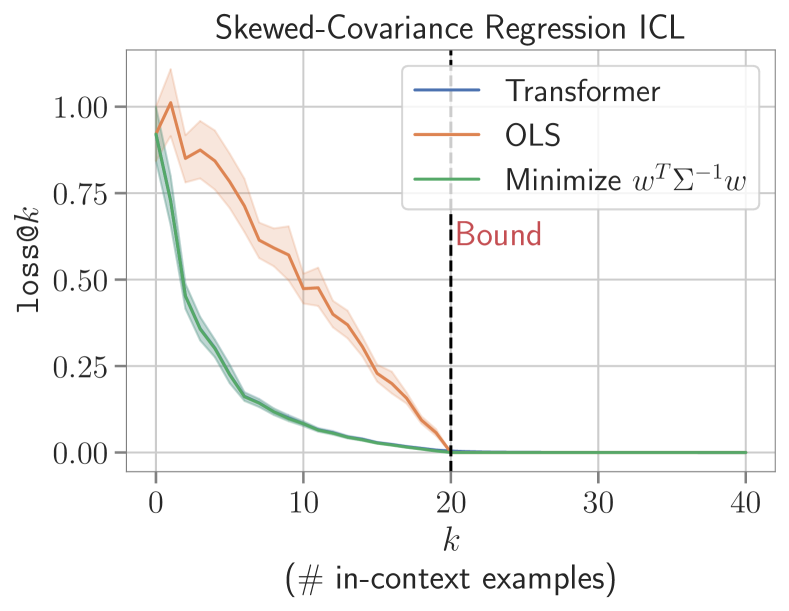
((a))

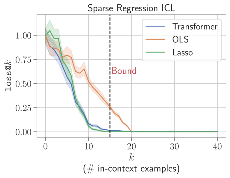
((b))

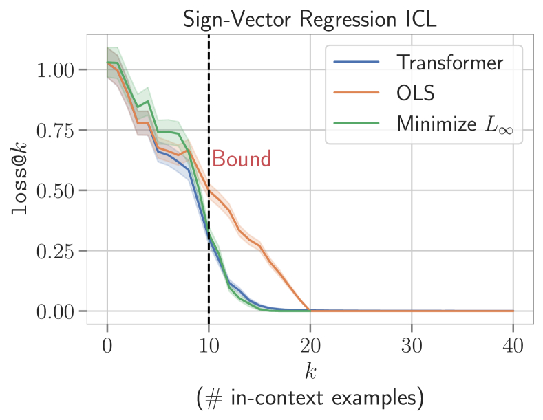
((c))

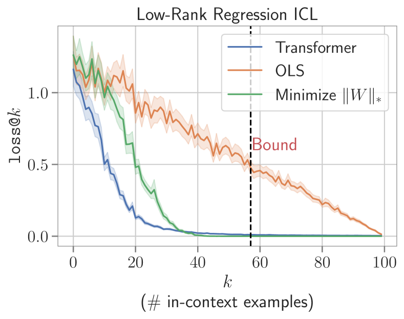
((d))

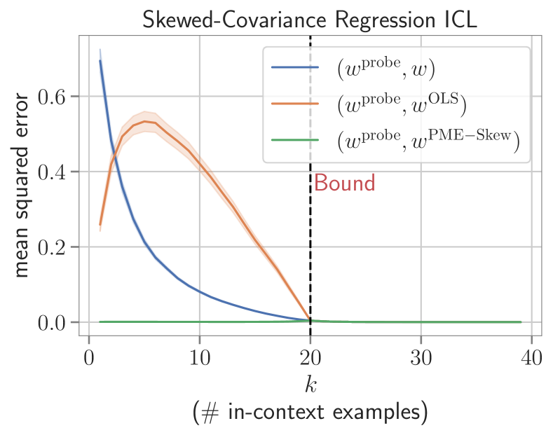
((e))

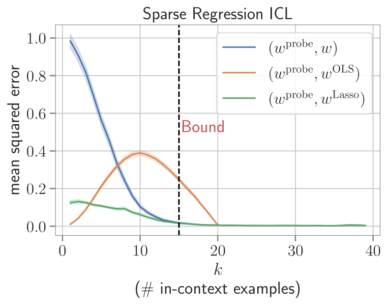
((f))

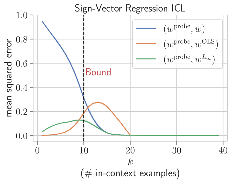
((g))

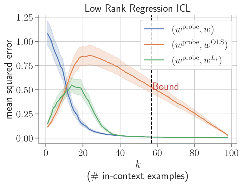
((h))

Figure 1: Comparing ICL in transformers for different linear functions with the relevant baselines. Top: $\texttt{loss@}k$ values for transformers and baselines on skewed covariance, sparse, sign-vector, and low-rank regression tasks. Bottom: Comparing the errors between the implicit weights recovered from transformers $w^{\text{probe}}$ with the ground truth weights $w$ and weights computed by different baselines. $\bm{\mathit{w}}^{\text{PME-Skew}}$ denotes the weights obtained by minimizing $\bm{\mathit{w}}^{T}\bm{\Sigma}^{-1}\bm{\mathit{w}}$ for the skewed covariance regression task.

Recovery bounds. For each function class above, there is a bound on the minimum number of in-context examples needed for the exact recovery of the solution vector $\bm{\mathit{w}}$. The bounds for sparse, sign-vector and low-rank regression are $2s\log(d/s)+5s/4$, $d/2$, and $3r(2q-r)$ respectively Chandrasekaran et al. (2012).

3.1.2 Results

We train transformer-based models on the five tasks following §2.1. Each model is trained with $d=20$ and $p=40$, excluding Low-Rank Regression where we train with $d=100$, $p=114$, and $r=1$. Figures 1(b)-1(d) compare the $\texttt{loss@}k$ values on these tasks with different baselines. Additionally, we also extract the implied weights $\bm{\mathit{w}}^{\mathrm{probe}}$ from the trained models when given a prompt $P$ following Akyürek et al. (2022) by generating model’s predictions $\{y^{\prime}_{i}\}$ on the test inputs $\{\bm{\mathit{x}}^{\prime}_{i}\}_{i=1}^{2d}\sim\mathcal{D}_{\mathcal{X}}$ and then solving the system of equations to recover $\bm{\mathit{w}}^{\mathrm{probe}}$. We then compare the implied weights $\bm{\mathit{w}}^{\mathrm{probe}}$ with the ground truth weights $\bm{\mathit{w}}$ as well as the weights extracted from different baselines to better understand the inductive biases exhibited by these models during in-context learning (Figures 1(f)-1(h)).

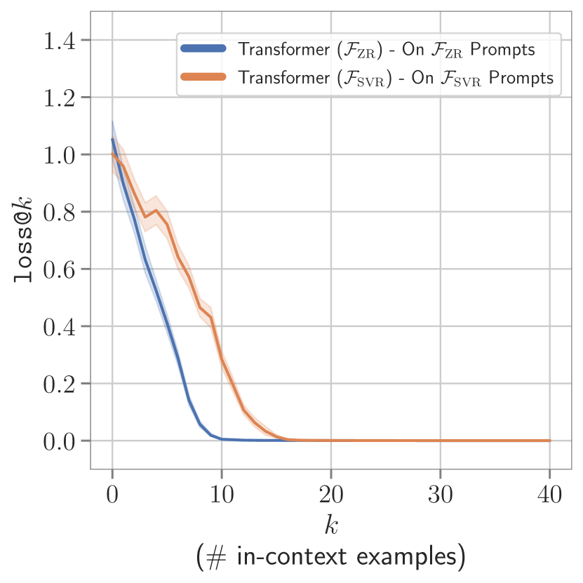
((a))

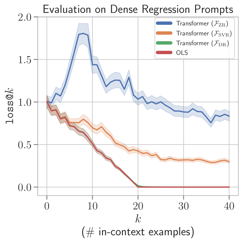
((b))

Figure 9: Evaluating transformer model trained for regression on task $\mathcal{F}_{\text{ZR}}$ with $\bm{\mathit{w}}\in\{\bm{\mathit{z}};\bm{\mathit{z}}\ |\ \bm{\mathit{z}}\in\{-2,-1,1,2\}^{10}\}$, not satisfying the convex geometry conditions of Chandrasekaran et al. [2012]. Left: Comparing the performance of this model, i.e. Transformer ($\mathcal{F}_{\text{ZR}}$), with Transformer ($\mathcal{F}_{\text{SVR}}$) when both are tested on their respective prompts. Right: Comparing the performance of Transformer ($\mathcal{F}_{\text{ZR}}$) with Transformer ($\mathcal{F}_{\text{SVR}}$) on Dense Regression ($\mathcal{F}_{\text{DR}}$) prompts. Transformer ($\mathcal{F}_{\text{ZR}}$) provides better performance than Transformer ($\mathcal{F}_{\text{SVR}}$) on in-distribution prompts but on OOD prompts (from $\mathcal{F}_{\text{DR}}$), Transformer ($\mathcal{F}_{\text{SVR}}$) performs better.

Since results for dense regression have been already covered in Akyürek et al. (2022), we do not repeat them here, but for completeness provide them in Figure 8 of Appendix. Refer to Figure 9 for the results on task $\mathcal{F}_{\text{ZR}}$. We observe that Transformers trained on this task ($\mathcal{F}_{\text{ZR}}$) provide better performance than those trained on Sign-Vector Regression ($\mathcal{F}_{\text{SVR}}$). Therefore, we can conclude that Transformers do not require any convexity conditions on weight vectors. For skewed-covariance regression, we observe that the transformer follows the PME solution very closely both in terms of the $\texttt{loss@}k$ values (Figure 1(a)) as well as the recovered weights for which the error between $\bm{\mathit{w}}^{\mathrm{probe}}$ and $\bm{\mathit{w}}^{\mathrm{PME-Skew}}$ (weights obtained by minimizing $\bm{\mathit{w}}^{T}\bm{\Sigma}^{-1}\bm{\mathit{w}}$) is close to zero at all prompt lengths (Figure 1(e)). On all the remaining tasks as well, the models perform better than OLS and are able to solve the problem with $<d$ samples i.e. underdetermined region meaning that they are able to understand the structure of the problem. The error curves of transformers for the tasks align closely with the errors of Lasso (Figure 1(b)), $L_{\infty}$ minimization (Figure 1(c)), and $L_{*}$ minimization (Figure 1(d)) baselines for the respective tasks. Interestingly for low-rank regression transformer actually performs better. Though, due to the larger problem dimension, ($d=100$) in this, it requires a bigger model: 24 layers, 16 heads, and 512 hidden size. In Figures 1(f), 1(g), and 1(h), we observe that at small prompt lengths $w^{\text{probe}}$ and $w^{\text{OLS}}$ are close. We conjecture that this might be attributed to both $w^{\text{probe}}$ and $w^{\text{OLS}}$ being close to $0$ for small prompt lengths (Figure 10 in Appendix). Prior distributions for all three tasks are centrally-symmetric, hence, at small prompt lengths when the posterior is likely to be close to the prior, the PME is close to the mean of the prior which is $0$. At larger prompt lengths transformers start to agree with $\bm{\mathit{w}}^{\mathrm{Lasso}}$, $\bm{\mathit{w}}^{L_{\infty}}$, and $\bm{\mathit{w}}^{L_{*}}$. This is consistent with the transformer following PME, assuming $\bm{\mathit{w}}^{\mathrm{Lasso}}$, $\bm{\mathit{w}}^{L_{\infty}}$, and $\bm{\mathit{w}}^{L_{*}}$ are close to PME—we leave it to future work to determine whether this is true (note that for sparse regression Lasso approximates the MAP estimate which should approach the PME solution as more data is observed).

3.2 Non-linear functions

Moving beyond linear functions, we now study how well transformers can in-context learn function classes with more complex relationships between the input and output, and if their behavior resembles the ideal learner i.e. the PME. Particularly, we consider the function classes of the form $\mathcal{F}_{\Phi}=\left\{f(\cdot;\Phi)|f(\bm{\mathit{x}};\Phi)=\bm{\mathit{w}}^{T}\Phi(\bm{\mathit{x}}),\bm{\mathit{w}}\in\mathbb{R}^{\Delta}\right\}$, where $\Phi:\mathbb{R}^{d}\rightarrow\mathbb{R}^{\Delta}$ maps the input vector $\bm{\mathit{x}}$ to an alternate feature representation. This corresponds to learning the mapping $\Phi(\bm{\mathit{x}})$ and then performing linear regression on top of it. Under the assumption of a standard Gaussian prior on $\bm{\mathit{w}}$, the PME for the dense regression can be easily extended for $\mathcal{F}_{\Phi}$: $\min_{\bm{\mathit{w}}}\|\bm{\mathit{w}}\|_{2}$, s.t. $\bm{\mathit{w}}^{T}\Phi(\bm{\mathit{x}}_{i})=f(\bm{\mathit{x}}_{i})$ for $i\in\{1,\cdots,p\}$.

In our experiments, we consider two such non-linear function classes, Fourier Series and Degree-2 Monomial Basis Regression. Below, we provide their description as well as results concerning the performance of transformers on these two classes.

3.2.1 Fourier Series

A Fourier series is an expansion of a periodic function into a sum of trigonometric functions. One can represent the Fourier series using the sine-cosine form given by:

$$f(x)=a_{0}+\sum_{n=1}^{N}a_{n}\cos{(n\pi x/L)}+\sum_{n=1}^{N}b_{n}\sin{(n\pi x/L)}$$

where, $x\in[-L,L]$, and $a_{0}$, $a_{n}$’s and $b_{n}$’s are known as Fourier coefficients and $\cos{n\pi/L}$ and $\sin{n\pi/L}$ define the frequency $n$ components. We can define the function class $\mathcal{F}_{\Phi_{N}}^{\text{fourier}}$ by considering $\Phi$ as the Fourier feature map i.e. $\Phi_{N}(x)=[1,\cos{({\pi x}/{L})},\cdots,\cos{({N\pi x}/{L})},\sin{({\pi x}/{L})},\cdots,\sin{({N\pi x}/{L})}]^{T}$, and $\bm{\mathit{w}}$ as Fourier coefficients: $\bm{\mathit{w}}=[a_{0},a_{1},\cdots,a_{N},b_{1},\cdots,b_{N}]$. Hence, $\Phi_{N}(x)\in\mathbb{R}^{d}$ and $\bm{\mathit{w}}\in\mathbb{R}^{d}$, where $d=2N+1$.

For training transformers to in-context-learn $\mathcal{F}_{\Phi_{N}}^{\text{fourier}}$, we fix a value of $N$ and sample functions $f\in\mathcal{F}_{\Phi_{N}}^{\text{fourier}}$ by sampling the Fourier coefficients from the standard normal distribution i.e. $\bm{\mathit{w}}\sim\mathcal{N}(\mathbf{0}_{d},\bm{\mathit{I}})$. We consider the inputs to be scalars, i.e. $x_{i}\in[-L,L]$ and we sample them i.i.d. from the uniform distribution on the domain: $x_{i}\sim\mathcal{U}(-L,L)$. In all of our experiments, we consider $N=10$ and $L=5$. At test time we evaluate on $\mathcal{F}_{\Phi_{M}}^{\text{fourier}}$ for $M\in[1,10]$, i.e. during evaluation we also prompt the model with functions with different maximum frequency as seen during training. As a baseline, we use OLS on the Fourier features (denoted as OLS Fourier Basis) which will be equivalent to the PME.

Measuring inductive biases. Once we train a transformer-based model to in-context learn $\mathcal{F}_{\Phi_{N}}^{\text{fourier}}$, how can we investigate the inductive biases that the model learns to solve the problem? We would like to answer questions such as, when prompted with $k$ input-output examples what are the prominent frequencies in the function simulated by the model, or, how do these exhibited frequencies change as we change the value of $k$? We start by sampling in-context examples $(x_{1},f(x_{1}),\cdots x_{k},f(x_{k}))$, and given the context obtain the model’s predictions on a set of $m$ test inputs $\{x^{\prime}_{i}\}_{i=1}^{m}$, i.e. $y^{\prime}_{i}=M_{\theta}\left(\bigl{(}x_{1},f(x_{1}),\cdots x_{k},f(x_{k}),x^{\prime}_{i}\bigl{)}\right)$. We can then perform Discrete Fourier Transform (DFT) on $\{y^{\prime}_{1},\cdots,y^{\prime}_{m}\}$ to obtain the Fourier coefficients of the function output by $M$, which we can analyze to understand the dominant frequencies.

Results. The results of our experiments concerning the Fourier series are provided in Figure 2. Transformers obtain $\texttt{loss@}k$ values close to the OLS Fourier Basis baseline (Figure 2(a)) indicating at least for the smaller prompt lengths the model is able to simulate the behavior of the ideal predictor (PME). Since the inputs $x_{i}$, in this case, are scalars, we can visualize the functions learned in context by transformers. We show one such example for a randomly selected function $f\sim\mathcal{F}_{\Phi_{M}}^{\text{fourier}}$ for prompting the model in Figure 2(b). As can be observed, the functions predicted by both the transformer and baseline have a close alignment, and both approach the ground truth function $f$ as more examples are provided. Finally, we visualize the distribution of the frequencies for the predicted functions in Figure 2(c). For a value of $M$, we sample 10 different functions and provide $k$ in-context examples to the model to extract the frequencies of the predicted functions using the DFT method. As can be observed, when provided with fewer in-context examples ($k=2$) both Transformer and the baseline predict functions with all the 10 frequencies (indicated by the values of $a_{n}^{2}+b_{n}^{2}$ in a similar range for $n\in[1,10]$), but as more examples are provided they begin to recognize the gold maximum frequency (i.e. $M=4$). We provide more detailed plots for all the combinations of $M$ and $k$ in Figures 11 and 12 of the Appendix. This suggests that the transformers are following the Bayesian predictor and are not biased towards smaller frequencies.

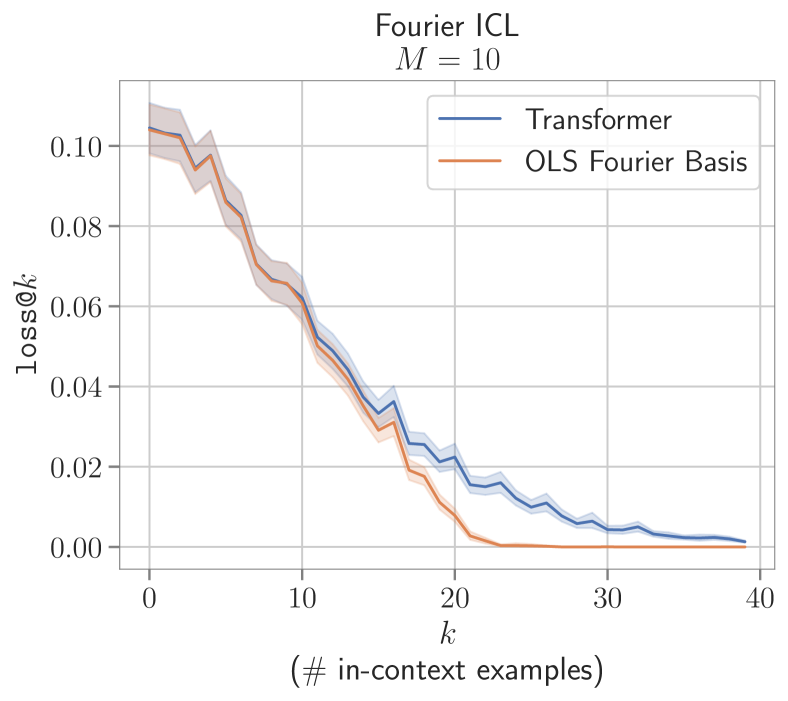
((a))

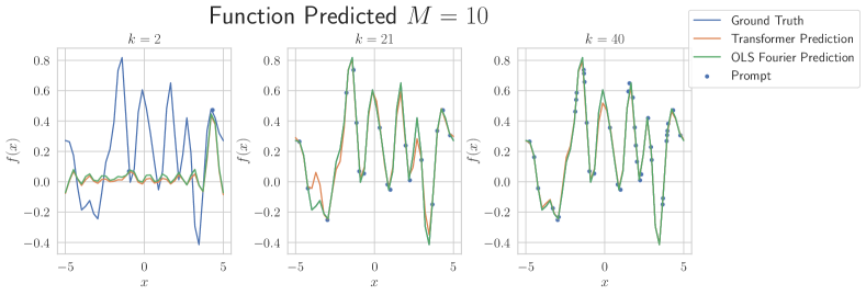
((b))

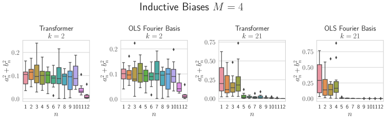
((c))

Figure 2: Effectiveness of ICL in transformers for Fourier series family of functions. Top left: $\texttt{loss@}k$ values for transformer and OLS Fourier Basis baseline. Top Right: Visualizing the functions simulated by the transformer and the OLS Fourier Basis. Bottom: Measuring the frequencies of the simulated function by the transformer and the baseline.

3.2.2 Random Fourier Features

Mapping input data to random low-dimensional features has been shown to be effective to approximate large-scale kernels Rahimi and Recht (2007). In this section, we are particularly interested in Random Fourier Features (RFF) which can be shown to approximate the Radial Basis Function kernel and are given as:

$$\Phi_{D}(\bm{\mathit{x}})=\sqrt{\frac{2}{D}}[\cos{(\bm{\omega}_{1}^{T}\bm{\mathit{x}}+\delta_{1})},\cdots,\cos{(\bm{\omega}_{D}^{T}\bm{\mathit{x}}+\delta_{D})}]^{T}$$

where $\bm{\omega}_{i}\in\mathbb{R}^{d}$ and $\delta_{i}\in\mathbb{R}$ $\forall i\in[1,D]$, such that $\Phi_{D}:\mathbb{R}^{d}\to\mathbb{R}^{D}$. Both $\bm{\omega}_{i}$ and $\delta$ are sampled randomly, such that $\bm{\omega}_{i}\in\mathcal{N}(\bm{\mathit{0}},\bm{\mathit{I}}_{d})$ and $\delta_{i}\in\mathcal{(}0,2\pi)$. We can then define the function family $\mathcal{F}^{\text{RFF}}_{\Phi_{D}}$ as linear functions over the random fourier features i.e. $f=\bm{\mathit{w}}^{T}\Phi_{D}(\bm{\mathit{x}})$ such that $f\sim\mathcal{F}^{\text{RFF}}_{\Phi_{D}}$. While training the transformer on this function class, we sample $\bm{\omega}_{i}$’s and $\delta_{i}$’s once and keep them fixed throughout the training. As a baseline, we use OLS over $(\Phi_{D}(x),y)$ pairs which will give the PME for the problem (denote this as RFF-OLS).

Results: For this particular family, we observed mixed results for transformers, i.e. they fail to generalize to functions of the family when the complexity of the problem is high. The complexity of this function class is dictated by the length of the $\bm{\omega}_{i}$ vectors (and the inputs $\bm{\mathit{x}}$) i.e. $d$ and the number of random features $D$. We plot the $\texttt{loss@}k$ values for transformer models trained on $\mathcal{F}^{\text{RFF}}_{\Phi_{D}}$ for different values of $d$ and $D$ in Figure 3. As can be observed, the complexity of the problem for the transformers is primarily governed by $d$, where they are able to solve the tasks for even large values of $D$, however, while they perform well for smaller values of $d$ ($d=1$ and $d=4$), for $d=10$, they perform much worse compared to the RFF-OLS baseline and the $\texttt{loss@}k$ doesn’t improve much once $\sim 15$ in-context examples are provided.

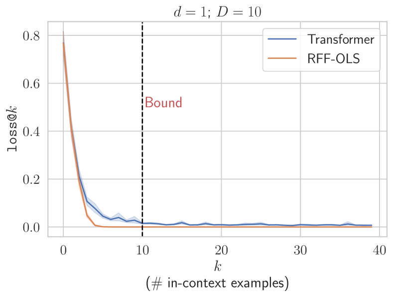
((a))

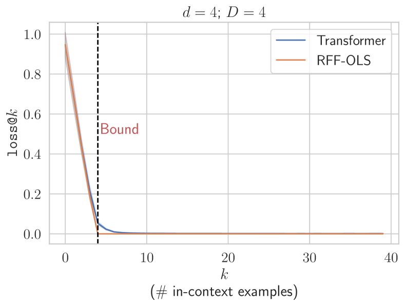
((b))

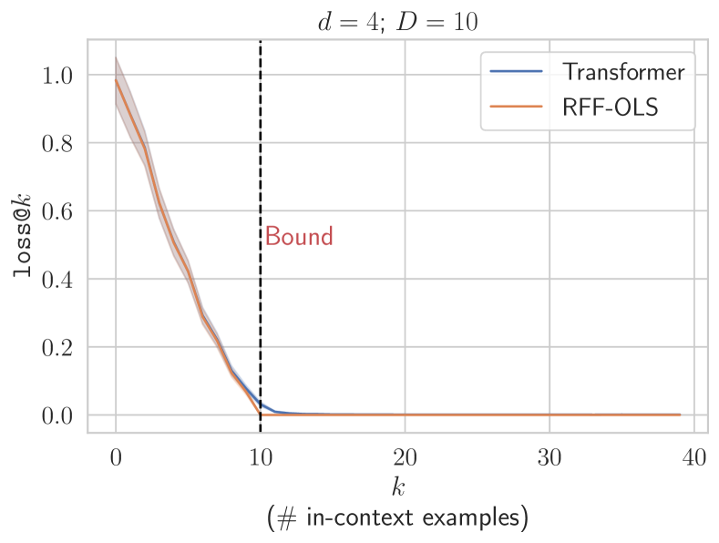
((c))

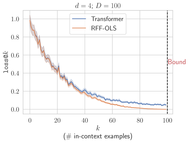
((d))

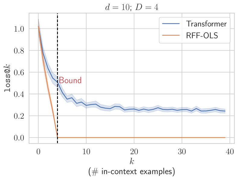
((e))

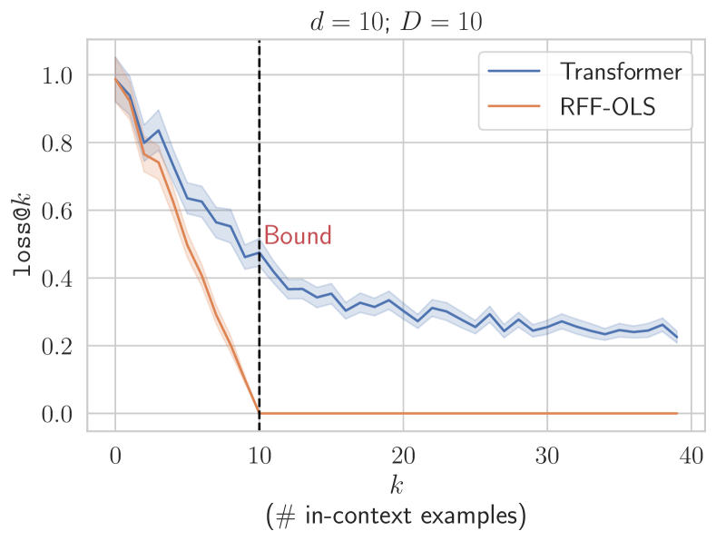
((f))

Figure 3: Comparing transformers performance on RFF function family ($\mathcal{F}^{\text{RFF}}_{\Phi_{D}}$) with the RFF-OLS baseline for different values of $d$ and $D$.

3.2.3 Degree-2 Monomial Basis Regression

We define a function family $\mathcal{F}_{\mathcal{S}}^{\text{mon.(2)}}$ with the basis formed by a subset $\mathcal{S}(\bm{\mathit{x}})$ of degree-2 monomials $\Phi_{M}(\bm{\mathit{x}})$ of any input $\bm{\mathit{x}}$. That is, $\mathcal{S}(\bm{\mathit{x}})\subset\Phi_{M}(\bm{\mathit{x}})=\{x_{i}x_{j}\ |\ 1\leq i,j\leq d\}$, and $f(\bm{\mathit{x}})=\bm{\mathit{w}}^{T}\mathcal{S}(\bm{\mathit{x}})$, where $\bm{\mathit{w}}\sim\mathcal{N}_{|\mathcal{S}|}(\bm{\mathit{0}},\bm{\mathit{I}})$. We compare the performance of transformers on this class with OLS performed on the basis $\mathcal{S}$ ($\text{OLS}_{\mathcal{S}}$). PME is given by the least $L_{2}$ norm solution and is hence equivalent to $\text{OLS}_{\mathcal{S}}$. We observe that the error curves of the transformer trained and evaluated on this family follow $\text{OLS}_{\mathcal{S}}$ baseline closely for all prompt lengths, both in-distribution and out-of-distribution. (Refer to §A.6 for a detailed description of the set-up and results.)

4 In-context learning of multiple function classes

While the original formulation by Garg et al. (2022) is for training transformers on a single class of functions, in our work we extend the in-context learning setup to multiple classes of functions. Formally, we define a task-mixture using a set of $m$ function classes $\mathcal{F}_{\mathcal{T}}=\{\mathcal{F}_{T_{1}},\cdots,\mathcal{F}_{T_{m}}\}$ corresponding to the set of tasks $\mathcal{T}=\{T_{1},\cdots,T_{m}\}$ (where $T_{i}$ represents a task such as DR, SR, SVR, etc.) and sampling probabilities $\bm{\alpha}=[\alpha_{1},\cdots\alpha_{m}]^{T}$ with $\sum_{i=1}^{m}\alpha_{i}=1$. We use $\bm{\alpha}$ to sample a task for constructing the training prompt $P$. We assume the input distribution $\mathcal{D}_{\mathcal{X}}$ to be same for each class $\mathcal{F}_{T_{i}}$. More concretely, the sampling process for $P$ is defined as:

$$T_{i}\sim\mathcal{T}~{}\text{s.t.}~{}\mathbb{P}(T=T_{i})=\alpha_{i}$$

$$f\sim\mathcal{F}_{T_{i}}$$

$$\bm{\mathit{x}}_{j}\sim\mathcal{D}_{\mathcal{X}},\forall j\in\{1,\cdots,p\}$$

Finally, $$P=\bigl{(}\bm{\mathit{x}}_{1},f(\bm{\mathit{x}}_{1}),\cdots\bm{\mathit{x}}_{p},f(\bm{\mathit{x}}_{p}),\bm{\mathit{x}}_{p+1}\bigl{)}$$

We can work out the PME for a task mixture, which is given by:

$$\small M_{\theta,\mathcal{T}}(P)=\beta_{1}M_{\theta,T_{1}}(P)+\ldots+\beta_{m}M_{\theta,T_{m}}(P),$$ (2)

where $\beta_{i}=\alpha_{i}p_{i}(P)/p_{\mathcal{T}}(P)$ for $i\leq m$. Probability density $p_{i}(\cdot)$ is induced by the task $T_{i}$ on the prompts in a natural way. Please refer to §A.1 in the Appendix for the derivation. The models are trained with the same objective as in Eq. 1, and at test time we evaluate $\texttt{loss@}k$ for each task individually.

4.1 Gaussian Mixture Models (GMMs)

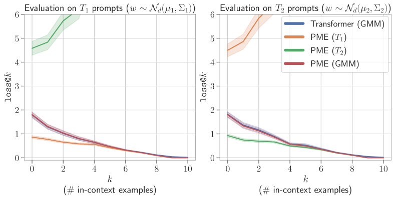
((a))

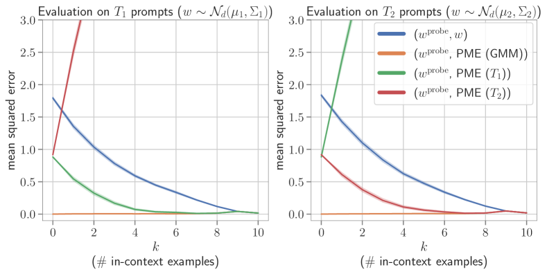
((b))

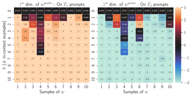
((c))

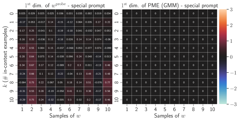
((d))

Figure 4: Transformers simulate PME when trained on dense regression task-mixture ($d=10,p=10,\alpha_{1}=\alpha_{2}=\frac{1}{2}$) with weights having a mixture of Gaussian prior (GMM). (a): Comparing the performance of the Transformer with Posterior Mean Estimator (PME) of individual Gaussian components (PME ($T_{1}$) and PME ($T_{2}$)) and of the mixture PME (GMM). (b): MSE between the probed weights of the Transformer and PMEs. (c): $1^{\text{st}}$ dimension of Transformer’s probed weights across the prompt length. (d): $1^{\text{st}}$ dimension of Transformer’s probed weights and PME (GMM) across the prompt length for a specially constructed prompt.

In the function classes discussed so far in this section, the computation of PME has not been discussed since it is usually intractable as it involves high-dimensional integrals. This subsection mitigates that gap by presenting a case where PME is tractable and provides quantitative evidence of transformers simulating PME. We design a Dense Regression task-mixture ($\mathcal{F}_{\{DR_{1},DR_{2}\}}$) where the prior on $\bm{\mathit{w}}$ is given by a mixture GMM of two Gaussians as follows:

$$p_{M}(\bm{\mathit{w}})=\alpha_{1}\mathcal{N}_{d}(\bm{\mu}_{1},\bm{\Sigma}_{1})+\alpha_{2}\mathcal{N}_{d}(\bm{\mu}_{2},\bm{\Sigma}_{2})$$

, where $\alpha_{1}+\alpha_{2}=1$. Note that this is equivalent to a task-mixture in §4 terminology where $\mathcal{T}=\{DR_{1},DR_{2}\}$, $DR_{1}$ and $DR_{2}$ both being DR tasks with different priors, and $\bm{\alpha}=[\alpha_{1},\alpha_{2}]^{T}$. For our experiments, the $d$-dimensional mean vectors are given by $\bm{\mu}_{1}=(3,0,..,0)$ and $\bm{\mu}_{2}=(-3,0,...,0)$ for the two Gaussian components of the mixture (call them $T_{1}$ and $T_{2}$ respectively). The covariance matrices are equal ($\bm{\Sigma}_{1}=\bm{\Sigma}_{2}=\bm{\Sigma}^{*}$), where $\Sigma^{*}$ is the identity matrix $\bm{I}_{d}$ with the top-left entry replaced by $0$. We train the transformer on two types of mixtures: (a) with equal mixture weights ($\alpha_{1}=\alpha_{2}=\frac{1}{2}$), (b) with unequal mixture weights ($\alpha_{1}=\frac{2}{3}$, $\alpha_{2}=\frac{1}{3}$). We use $d=10$ and $p$ (prompt length) $=\{10,20\}$ and utilize curriculum for $d$ and $p$ as given in Table 1.

Results. Figure 4 shows the squared errors between different predictors and ground truth, along with their weights. In Figure 4(a), we note that Transformer’s error trends almost exactly align with those of the PME of the mixture, PME (GMM), when prompts come from either $T_{1}$ or $T_{2}$. For each plot, let $T_{\mathrm{prompt}}$  and $T_{\mathrm{other}}$  denote the component from which prompts are provided and the other component respectively. When $d(=10)$ examples from $T_{\mathrm{prompt}}$  have been provided, the Transformer, PME ($T_{\mathrm{prompt}}$), and PME (GMM) all converge to the same minimum error of 0. This shows that Transformer is simulating PME (GMM), which converges to PME ($T_{\mathrm{prompt}}$) at $k=d$. PME ($T_{\mathrm{other}}$)’s errors keep increasing as more examples are provided. These observations are in line with Eq. 4: As more examples from the prompt are observed, the weights of individual PMEs used to compute the PME (GMM) (i.e. the $\beta$’s) adjust themselves such that the contribution of $T_{\mathrm{prompt}}$  increases in the mixture with $k$ (Figure 16 in the Appendix shows this more evidently). In Figure 4(b), MSE between weights from different predictors are plotted. For Transformer, we obtain these weights $\bm{\mathit{w}}^{\mathrm{probe}}$ by probing using the procedure mentioned in §3.1.2. Transformer’s weights are almost exactly identical to PME (GMM) $\forall k\in\{1,2,\cdots,p\}$. This is another concrete evidence that it is simulating PME (GMM). Initially (at $k=0$), when no information about the prompt is known, the Transformer’s weights ($\bm{\mathit{w}}^{\mathrm{probe}}$) are close to those of both PME ($T_{1}$) and PME ($T_{2}$), giving the same error. But as $k$ increases and more examples are provided, $\bm{\mathit{w}}^{\mathrm{probe}}$ converges to PME ($T_{\mathrm{prompt}}$) and diverges from PME ($T_{\mathrm{other}}$). At $k=d$, the ground truth weights $\bm{\mathit{w}}$, PME (GMM), PME ($T_{\mathrm{prompt}}$), and Transformer weights $\bm{\mathit{w}}^{\mathrm{probe}}$ all converge to the same value. Figure 4(c) shows the evolution of the first dimension of the Transformer weights, i.e. $(\bm{\mathit{w}}^{\mathrm{probe}})_{1}$, with prompt length $k$. We see that Transformer is simulating PME (GMM), which approaches PME ($T_{\mathrm{prompt}}$) with increasing prompt length ($k$). Note that PME (GMM) approaches PME ($T_{\mathrm{prompt}}$) with increasing $k$ (Eq. 4). Also note that in our setting, regardless of $k$ the first dimension of PME ($T_{i}$) is $(\bm{\mu}_{i})_{1}$, the first dimension of the mean of the prior distribution $T_{i}$, since $T_{i}$ has a fixed value (i.e. zero variance) in the first dimension. Hence, if Transformer is simulating PME (GMM), the first dimension of Transformer’s weights $(\bm{\mathit{w}}^{\mathrm{probe}})_{1}$ must approach $(\bm{\mu}_{1})_{1}$ (when $T_{\mathrm{prompt}}$ $=T_{1}$) and $(\bm{\mu}_{2})_{1}$ (when $T_{\mathrm{prompt}}$ $=T_{2}$). This is exactly what we observe as $(\bm{\mathit{w}}^{\mathrm{probe}})_{1}$ approaches $+3$ and $-3$ on $T_{1}$ and $T_{2}$ prompts respectively. At prompt length $0$, in the absence of any information about the prompt, $(\bm{\mathit{w}}^{\mathrm{probe}})_{1}$ $\approx 0$. This agrees with Eq. 4 since $0=(\bm{\mu}_{1})_{1}.\beta_{1}+(\bm{\mu}_{2})_{1}.\beta_{2}$, where $(\bm{\mu}_{1})_{1}=+3,(\bm{\mu}_{2})_{1}=-3,\beta_{1}=\alpha_{1}=0.5$ and $\beta_{2}=\alpha_{2}=0.5$ when prompt $P$ is empty. The figure shows that with the increasing evidence from the prompt, the transformer shifts its weights to $T_{\mathrm{prompt}}$’s weights as evidenced by the first coordinate changing from $0$ to $+3$ or $-3$ based on the prompt. Lastly, in Figure 4(d), we check the behavior of Transformer and PME (GMM) on specially constructed prompts $P$ where $(\bm{\mathit{x}}_{i})_{1}=0$ and $(\bm{\mathit{x}}_{i})_{2:d}\sim\mathcal{N}(0,1),\forall i\in\{1,\cdots,p\}$. For our setup, choosing such $\bm{\mathit{x}}_{i}$’s guarantees that no information about the distribution of $\bm{\mathit{w}}$ becomes known by observing $P$ (since the only distinguishing dimension between $T_{1}$ and $T_{2}$ is the $1^{\mathrm{st}}$ dimension and that does not influence the prompt in this case as $(\bm{\mathit{x}}_{i})_{1}=0$). We note that Transformer’s weights are all $\approx 0$ regardless of the prompt length, agreeing with the PME (GMM). Observing more examples from the prompt does not reveal any information about the underlying distribution of $\bm{\mathit{w}}$ in this case. All of this evidence strongly supports our hypothesis that Transformer behaves like the ideal learner and computes the Posterior Mean Estimate (PME). The results of the mixture with unequal weights ($\alpha_{1},\alpha_{2}$) for $T_{1}$ and $T_{2}$ and for $p=20$ model further strengthen this evidence. Please refer to §A.8 for these results.

4.2 ICL on task mixtures

We start by training transformer models on the mixture of linear regression tasks discussed in §3.1. We consider binary mixtures of Dense Regression and Sparse Regression ($\mathcal{F}_{\{\text{DR, SR}\}}$), Dense Regression and Sign-Vector Regression ($\mathcal{F}_{\{\text{DR, SVR}\}}$), and Dense Regression and Skewed-Covariance Regression ($\mathcal{F}_{\{\text{DR, Skew-DR}\}}$) as well as the tertiary mixture consisting of all three tasks ($\mathcal{F}_{\{\text{DR, SR, SVR}\}}$). Unless specified we consider the mixtures to be uniform i.e. $\alpha_{i}=\frac{1}{|\mathcal{T}|}$ for all $T\in\mathcal{T}$ and use these values to sample batches during training. We also explore more complex mixtures like dense regression and decision tree mixture $\mathcal{F}_{\{\text{DR, DT}\}}$ and decision tree and neural network mixture $\mathcal{F}_{\{\text{DT, NN}\}}$.

During the evaluation, we test the mixture model (denoted as Transformer $\mathcal{F}_{\mathcal{T}}$) on the prompts sampled from each of the function classes in the mixture. We consider the model to have in-context learned the mixture of tasks if it obtains similar performance as the single-task models specific to these function classes. For example, a transformer model trained on the dense and sparse regression mixture (Transformer $\mathcal{F}_{\{\text{DR, SR}\}}$) should obtain performance similar to the single-task model trained on dense regression function class (Transformer $\mathcal{F}_{\text{DR}}$), when prompted with a function $f\sim\mathcal{F}_{\text{DR}}$ and vice-versa. We have consistent observations for all of these mixtures, so we discuss only $\mathcal{F}_{\{\text{DR, SR}\}}$ here in detail, while the results for the other mixtures can be found in §A.9 of the Appendix.

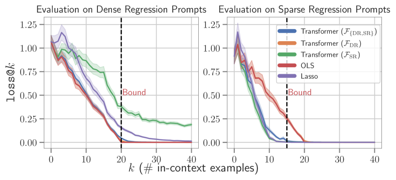
((a))

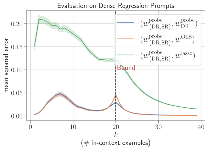
((b))

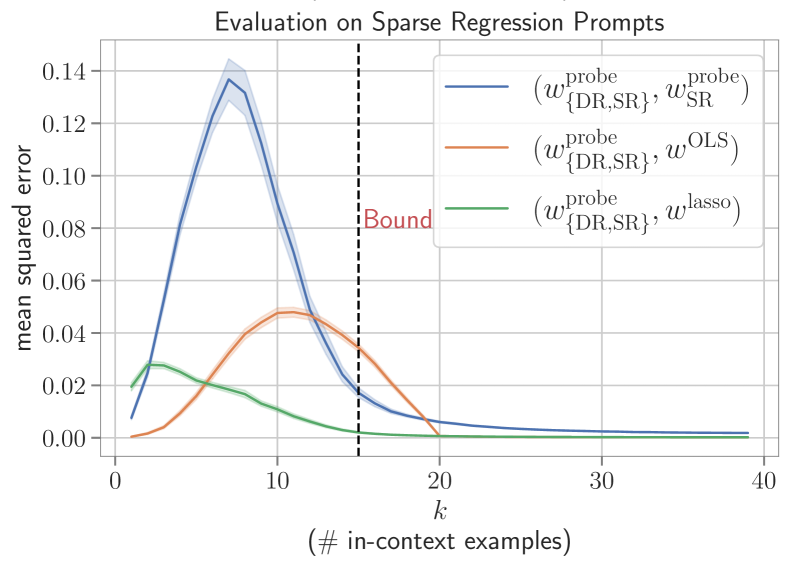
((c))

Figure 5: Comparing the performance of a Transformer model trained on dense and sparse regression mixture $\mathcal{F}_{\{\text{DR, SR}\}}$ with baselines, as well as single task models, trained on $\mathcal{F}_{\text{DR}}$ and $\mathcal{F}_{\text{SR}}$ individually.

Results. The results for the binary mixtures of linear functions are given in Figure 5. As can be observed in Figure 5(a), the transformer model trained on $\mathcal{F}_{\{\text{DR, SR}\}}$ obtains performance close to the OLS baseline as well as the transformer model specifically trained on the dense regression function class $\mathcal{F}_{\text{DR}}$ when evaluated with dense regression prompts. On the other hand, when evaluated with sparse regression prompts the same model follows Lasso and single-task sparse regression model (Transformer ($\mathcal{F}_{\text{SR}}$)) closely. As a check, note that the single-task models when prompted with functions from a family different from what they were trained on, observe much higher errors, confirming that the transformers learn to solve individual tasks based on the in-context examples provided. We also recovered the weights from the multi-task models using the same method as discussed in §3.1 when given prompts from each function class and measure how well they agree with the gold baselines as well as the single-task models trained on individual tasks. We denote weights recovered from the multi-task models as $w^{\text{probe}}_{\mathcal{T}}$ and the ones from single task models as $w^{\text{probe}}_{T_{i}}$ when trained on task $T_{i}$. In Figures 5(b) and 5(c) we report results for the $\mathcal{F}_{\{\text{DR, SR}\}}$ mixture and we observe that the weights recovered by the mixture model start to agree with task-wise models once sufficient in-context examples are provided (more or less close to the recovery bound) while the errors are high initially. Interestingly, we observe for very low prompt lengths ($k<5$), the errors tend to be small, which can be explained by the similar reasoning as in §3.1 i.e. the priors for both tasks being centrally symmetric. These observations are consistent with the hypothesis that transformers compute PME (assuming transformers trained on single tasks simulate the PME).

Conditions affecting multi-task in-context learning. In some of our initial experiments with $\mathcal{F}_{\{\text{DR, SR}\}}$ mixture transformers failed to learn to solve the individual tasks of the mixture and were following OLS for both $\mathcal{F}_{\text{DR}}$ and $\mathcal{F}_{\text{SR}}$ prompts. To probe this, we first noted that the variance of the function outputs varied greatly for the two tasks, where for dense regression it equals $d$ and equals the sparsity parameter $s$ for sparse regression. We hypothesized that the model learning to solve just dense regression might be attributed to the disproportionately high signal from dense regression compared to sparse. To resolve this, we experimented with increasing the sampling rate for the $\mathcal{F}_{\text{SR}}$ task family during training. Particularly on training the model with $\alpha_{\text{SR}}=0.87$, we observed that the resulting model did learn to solve both tasks. Alternatively, normalizing the outputs of the two tasks such that they have the same variance and using a uniform mixture ($\alpha_{\text{SR}}=0.5$) also resulted in multi-task in-context learning capabilities (also the setting of our experiments in Figure 5). Hence, the training distribution can have a significant role to play in the model acquiring abilities to solve different tasks as has been also observed in other works on in-context learning in LLMs Razeghi et al. (2022); Chan et al. (2022a).

We also studied if the curriculum had any role to play in the models acquiring multi-task in-context learning capabilities. In our initial experiments without normalization and non-uniform mixtures, we observed that the model only learned to solve both tasks when the curriculum was enabled. However, training the model without curriculum for a longer duration ($\approx$ more training data), we did observe it to eventually learn to solve both of the tasks indicated by a sharp dip in the evaluation loss for the sparse regression task during training. This is also in line with recent works Hoffmann et al. (2022); Touvron et al. (2023), which show that the capabilities of LLMs can be drastically improved by scaling up the number of tokens the models are trained on. Detailed results concerning these findings are in Figure 25 of the Appendix.

4.3 Simplicity bias in ICL?

We consider a mixture of Fourier series function classes with different maximum frequencies, i.e. $\mathcal{F}_{\Phi_{1:N}}^{\text{fourier}}=\{\mathcal{F}_{\Phi_{1}}^{\text{fourier}},\cdots,\mathcal{F}_{\Phi_{N}}^{\text{fourier}}\}$. We consider $N=10$ in our experiments and train the models using a uniform mixture with normalization. During evaluation, we test individually on each $\mathcal{F}_{\Phi_{M}}^{\text{fourier}}$, where $M\in[1,N]$. We compare against consider two baselines: i) OLS Fourier Basis $\mathcal{F}_{\Phi_{M}}^{\text{fourier}}$ i.e. performing OLS on the basis corresponding to the number of frequencies $M$ in the ground truth function, and ii) $\mathcal{F}_{\Phi_{N}}^{\text{fourier}}$ which performs OLS on the basis corresponding to the maximum number of frequencies in the mixture i.e. $N$.

Figure 6(a) plots the $\texttt{loss@}k$ metric aggregated over all the $M\in[1,N]$ for the model and the baselines. The performance of the transformer lies somewhere in between the gold-frequency baseline (OLS Fourier Basis $\mathcal{F}_{\Phi_{M}}^{\text{fourier}}$) and the maximum frequency baseline ($\mathcal{F}_{\Phi_{N}}^{\text{fourier}}$), with the model performing much better compared to the latter for short prompt lengths ($k<20$) while the former baseline performs better. We also measure the frequencies exhibited by the functions predicted by the transformer in Figure 6(b). We observe that transformers have a bias towards lower frequencies when prompted with a few examples; however, when given sufficiently many examples they are able to recover the gold frequencies. This simplicity bias can be traced to the training dataset for the mixture since lower frequencies are present in most of the functions of the mixture while higher frequencies will be more rare: Frequency $1$ will be present in all the function classes whereas frequency $N$ will be present only in $\mathcal{F}_{\Phi_{N}}^{\text{fourier}}$. Our results indicate that the simplicity bias in these models during in-context learning arises from the training data distribution.

To further verify this observation, we also consider the case where the training data is biased towards high frequencies and check if transformers trained with such data exhibit bias towards high frequencies (complexity bias). To motivate such a mixture, we first define an alternate fourier basis: $\Phi_{n_{0},N}(x)=[\cos{(n_{0}\pi/L)},\sin{(n_{0}\pi/L)},\cos{((n_{0}+1)\pi/L)},\sin{((n_{0}+1)\pi/L)},\cdots,\cos{(N\pi/L)},\sin{(N\pi/L)}]$, where $n_{0}\geq 0$ is the minimum frequency in the basis. $\Phi_{n_{0},N}$ defines the function family $\mathcal{F}^{fourier}_{\Phi_{n_{0},N}}$ and equivalently we can define the mixture of such function classes as $\mathcal{F}_{\Phi_{1:N,N}^{fourier}}=\{\mathcal{F}^{fourier}_{\Phi_{1,N}},\cdots,\mathcal{F}^{fourier}_{\Phi_{N,N}}\}$. One can see such a mixture will be biased towards high frequency; frequency $N$ is present in each function class of the mixture, while frequency $1$ is only present in $\mathcal{F}^{fourier}_{\Phi_{1,N}}$. We train a transformer model on such a mixture for $N=5$ and at test time, we evaluate the model on functions $f\sim\mathcal{F}^{fourier}_{\Phi_{m_{0},M}}$ Figure 6(c) shows the inductive biases measure from this trained model and we can clearly observe a case of complexity bias, where at small prompt lengths, the model exhibited a strong bias towards the higher end of the frequencies that it was trained on i.e. close to $5$.

We also trained models for higher values of the maximum frequency i.e. $N=10$ for the high-frequency bias case, but interestingly observed the model failed to learn this task mixture. Even for $N=5$, we noticed that the convergence was much slower compared to training on the simplicity bias mixture $\mathcal{F}_{\Phi_{1:N}}^{fourier}$. This indicates, while in this case, the origin of simplicity bias comes from the training data, it is harder for the model to learn to capture more complex training distributions, and simplicity bias in the pre-training data distribution might lead to more efficient training Mueller and Linzen (2023).

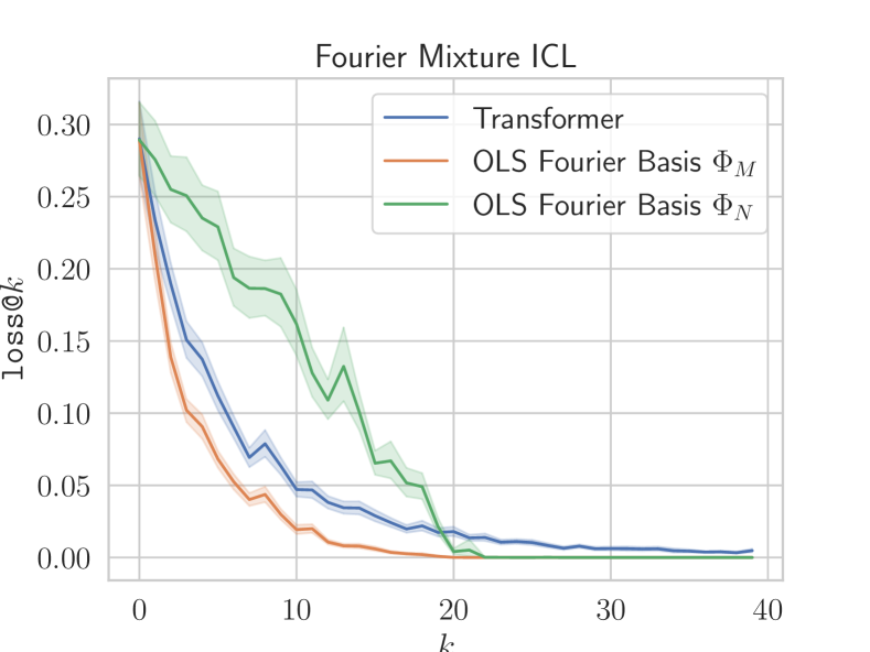
((a))

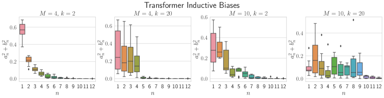
((b))

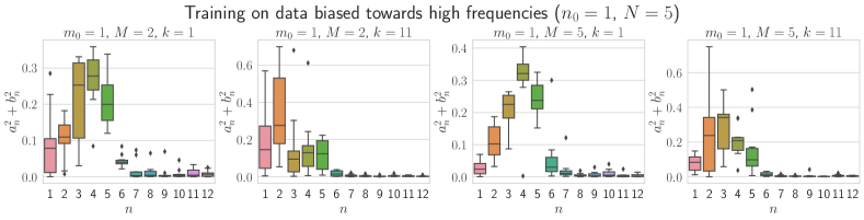
((c))

Figure 6: In-context learning on the Fourier series mixture class. Top Left: Comparing transformers with the baselines. Errors are computed on batches of 128 for $M\in[1,10]$ and aggregated in the plot. Top Right: Visualizing the frequencies of the simulated function by transformers. Bottom: Training transformer on high-frequency biased Fourier mixture $\mathcal{F}_{\Phi_{1:N,N}^{fourier}}$ and visualizing the simulated frequencies of the trained model.

5 Conclusion

We showed evidence of high-capacity transformers simulating the behavior of an ideal learner for various families of functions as well as their mixtures in the new MICL framework. Some of the key takeaways from our work include:

1. We show for a variety of single-task function classes like Skewed-Covariance Regression, Fourier Series, and Random Fourier Features as well as the mixture of tasks like Gaussian Mixture models that transformers are able to learn the PME solution for these problems. We verify this by not only comparing the errors of transformers with the PME but also investigating the inductive biases captured by these models and comparing them with those of ideal learners.

2. For tasks where the computation of PME is intractable, we compare the performance of transformers with strong baselines for these tasks and show transformers either outperform or obtain similar performances to these algorithms, hinting that these models might be simulating the behavior of ideal learners for these tasks. Specifically for linear inverse problems, we observe transformers are able to capture the structure of the problem, like the sparsity or low-rank parameterization of the ground truth function.

3. For the multi-task case, we show that transformers depending on the task from which in-context examples are sampled obtain similar performance as single-task models individually trained on these tasks. While we show transformers exhibiting the multi-task ICL behavior for a variety of problems, we also notice that the training data distribution as well as the amount of training data can dictate the emergence of this property.

4. Finally, through our experiments on mixtures of Fourier series function classes, we showed that the simplicity bias during ICL in transformers can be traced back to training distribution. Particularly, we observed that transformers exhibit bias towards low frequencies when the training data is itself biased towards low frequencies and observe the inverse behavior when the training data is biased towards high frequencies. We also note that transformers might struggle to learn function classes with more complex training distributions like in the case of the RFF tasks with increasing values of $d$ as well as for the complexity bias Fourier series task with large values of $N$.

There are many interesting directions for future work. Because of the difficulties in computing PME, we were not able to conclusively establish in many cases that the transformers do Bayesian prediction. It is an interesting theoretical challenge to resolve this. While we showed that for many problems, including non-linear ones, transformers achieve small ICL errors, this is not true for classes like neural networks and decision trees. This presumably happens because of computational as well as information-theoretic difficulties with the harder function classes. Despite this transformers achieve interesting results. How can we explain this from a Bayesian perspective? Also, most of the evaluations in our work focused on drawing functions at test time from the same distribution as seen during training. While we perform some OOD evaluations particularly for Fourier series (where we evaluate on different maximum frequencies as seen during training) and for Degree-2 monomial basis regression tasks (details in Appendix §A.6), a more rigorous OOD testing to check the validity of our results is an important future direction. Finally, in this paper, we treated transformers as black boxes: opening the box and uncovering the underlying mechanisms transformers use to do Bayesian prediction would be very interesting.

Appendix A Appendix

A.1 PME Theoretical Details

We mentioned earlier that an ideal LM would learn the pretraining distribution. This happens when using the cross-entropy loss. Since we use the square loss in (1), the predictions of the model can be computed using the posterior mean estimator (PME) from Bayesian statistics. For each prompt length $i$ we can compute PME by taking the corresponding summand in (1)

$$\min_{\theta}\operatorname*{\mathbb{E}}_{f,\bm{\mathit{x}}_{1:i}}\;\ell\left(M_{\theta}(P^{i}),f(\bm{\mathit{x}}_{i+1})\right) =\min_{\theta}\operatorname*{\mathbb{E}}_{f,P^{i}}\;\ell\left(M_{\theta}(P^{i}),f(\bm{\mathit{x}}_{i+1})\right)$$

$$=\min_{\theta}\operatorname*{\mathbb{E}}_{P^{i}}\;\operatorname*{\mathbb{E}}_{f}\left[\ell\left(M_{\theta}(P^{i}),f(\bm{\mathit{x}}_{i+1})\right)\,|\,P^{i}\right]$$

$$=\operatorname*{\mathbb{E}}_{P^{i}}\;\min_{\theta}\operatorname*{\mathbb{E}}_{f}\left[\ell\left(M_{\theta}(P^{i}),f(\bm{\mathit{x}}_{i+1})\right)\,|\,P^{i}\right].$$

The inner minimization is seen to be achieved by $M_{\theta}(P^{i})=\operatorname*{\mathbb{E}}_{f}\left[f(\bm{\mathit{x}}_{i+1})\,|\,P^{i}\right]$. This is the optimal solution for prompt $P^{i}$ and what we refer to as PME.

PME for a task mixture.

We describe the PME for a mixture of tasks. For simplicity we confine ourselves to mixtures of two tasks; extension to more tasks is analogous. Let $T_{1}$ and $T_{2}$ be two tasks specified by probability distributions $\mathcal{D}_{\mathcal{F}_{1}}$ and $\mathcal{D}_{\mathcal{F}_{2}}$, resp. As in the single task case, the inputs $\bm{\mathit{x}}$ are chosen i.i.d. from a common distribution $\mathcal{D}_{\mathcal{X}}$. For $\alpha_{1},\alpha_{2}\in[0,1]$ with $\alpha_{1}+\alpha_{2}=1$ a $(\alpha_{1},\alpha_{2})$-mixture $T$ of $T_{1}$ and $T_{2}$ is the task in which the prompt $P=\bigl{(}\bm{\mathit{x}}_{1},f(\bm{\mathit{x}}_{i}),\cdots,\bm{\mathit{x}}_{p},f(\bm{\mathit{x}}_{p}),\bm{\mathit{x}}_{p+1}\bigl{)}$ is constructed by first picking task $T_{i}$ with probability $\alpha_{i}$ for $i\in\{1,2\}$ and then picking $f\sim\mathcal{D}_{\mathcal{F}_{i}}$. Thus $p_{T}(f)=\alpha_{1}p_{T_{1}}(f)+\alpha_{2}p_{T_{2}}(f)$ where $p_{T}(\cdot)$ is the probability density under task $T$ which defines $\mathcal{D}_{T}$. For conciseness in the following we use $p_{1}(\cdot)$ for $p_{T_{1}}(\cdot)$ etc. Now recall that PME for task $T$ is given by

$$M_{\theta,T}(P) =\operatorname*{\mathbb{E}}_{f\sim\mathcal{D}_{T}}\left[f(\bm{\mathit{x}}_{p+1})\,|\,P\right]=\int p_{T}(f|P)\,f(x)\,\mathrm{d}f.$$ (3)

We would like to compute this in terms of PMEs for $T_{1}$ and $T_{2}$. To this end, we first compute

$$p_{T}(f|P) =\frac{p_{T}(P|f)p_{T}(f)}{p_{T}(P)}=\frac{p(P|f)p_{T}(f)}{p_{T}(P)}=\frac{p(P|f)}{p_{T}(P)}\big{[}\alpha_{1}p_{1}(f)+p_{2}(f)\big{]}$$

$$=\frac{\alpha_{1}p_{1}(P)}{p_{T}(P)}\frac{p(P|f)p_{1}(f)}{p_{1}(P)}+\frac{\alpha_{2}p_{2}(P)}{p_{T}(P)}\frac{p(P|f)p_{T_{2}}(f)}{p_{T_{2}}(P)}$$

$$=\frac{\alpha_{1}p_{1}(P)}{p_{T}(P)}p_{1}(f|P)+\frac{\alpha_{2}p_{2}(P)}{p_{T}(P)}p_{2}(f|P)$$

$$=\beta_{1}\,p_{1}(f|P)+\beta_{2}\,p_{2}(f|P),$$

where $\beta_{1}=\frac{\alpha_{1}p_{1}(P)}{p_{T}(P)}$ and $\beta_{2}=\frac{\alpha_{2}p_{2}(P)}{p_{T}(P)}$. Plugging this in (3) we get

$$M_{\theta,T}(P)=\beta_{1}\int p_{1}(f|P)\,f(x)\,\mathrm{d}f+\beta_{2}\int p_{2}(f|P)\,f(x)\,\mathrm{d}f=\beta_{1}M_{\theta,T_{1}}(P)+\beta_{2}M_{\theta,T_{2}}(P).$$ (4)

A.2 The curious case of positional encodings.

Positional encodings both learnable or sinusoidal in transformer architectures have been shown to result in poor length generalization Bhattamishra et al. [2020], Press et al. [2022], i.e. when tested on sequences of lengths greater than those seen during training the performance tends to drop drastically. In our initial experiments, we observed this issue with length generalization in our in-context-learning setup as well (Figure 7). While there are now alternatives to the originally proposed position encodings like Rotary Embeddings Su et al. [2021] and ALiBi Press et al. [2022] which perform better on length generalization, we find that something much simpler works surprisingly well in our setup. We found that removing position encodings significantly improved the length generalization for both dense and sparse linear regression while maintaining virtually the same performance in the training regime as can be seen in Figure 7. These observations are in line with Bhattamishra et al. [2020] which shows that decoder-only transformers without positional encodings fare much better in recognizing formal languages as well as Haviv et al. [2022] that shows transformers language models without explicit position encodings can still learn positional information. Both works attribute this phenomenon to the presence of the causal mask in decoder-only models which implicitly provides positional information to these models. Hence by default in all our experiments, unless specified, we do not use any positional encodings while training our models.

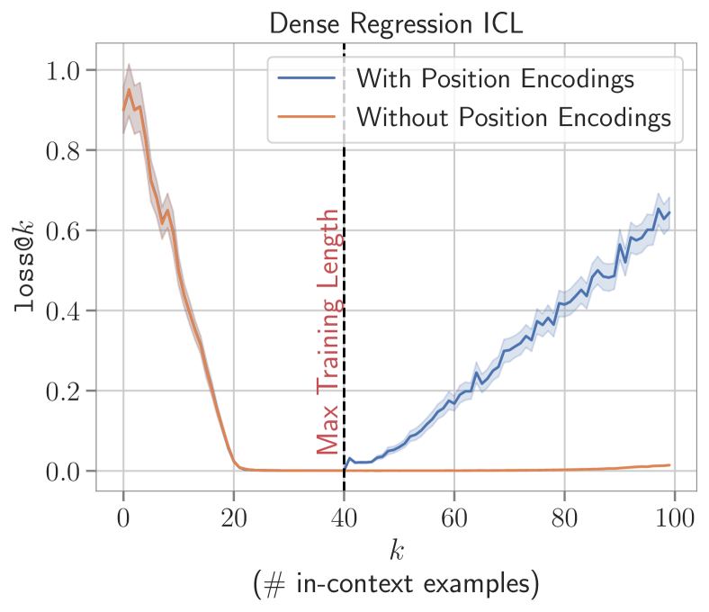
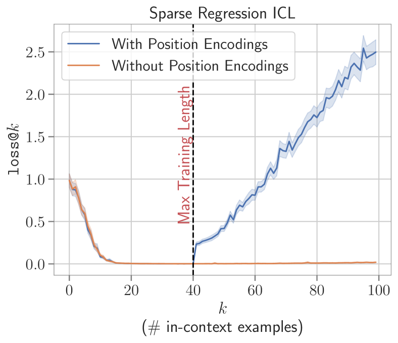
Figure 7: Impact of positional encodings on length generalization during in-context learning for dense and sparse linear regression tasks. For both tasks, the model was trained with $p=40$ i.e. the maximum number of in-context examples provided.

A.3 Experimental Setup

We use Adam optimizer Kingma and Ba [2015] to train our models. We train all of our models with curriculum and observe that curriculum helps in faster convergence, i.e., the same optima can also be achieved by training the model for more training steps as also noted by Garg et al. [2022]. Table 1 states the curriculum used for each experiment, where the syntax followed for each column specifying curriculum is [start, end, increment, interval]. The value of the said attribute goes from start to end, increasing by increment every interval train steps. Our experiments were conducted on a system comprising 32 NVIDIA V100 16GB GPUs. The cumulative training time of all models for this project was $\sim$ 30,000 GPU hours. While reporting the results, the error is averaged over 1280 prompts and shaded regions denote a 90% confidence interval over 1000 bootstrap trials.

Table 1: The values of curriculum attributes used for each experiment. $C_{d},C_{p}$ and $C_{\textrm{freq}}$ denote the curriculum on number of input dimensions ($d$), number of points ($p$) and any other experiment-specific attribute respectively. For Fourier Series $C_{\textrm{freq}}$ refers to maximum frequency $N$)

Experiment	Section	$C_{d}$	$C_{p}$	$C_{\textrm{freq}}$
Dense, Sparse and Sign-Vector Regression	§3.1.1	$[5,20,1,2000]$	$[10,40,2,2000]$	n/a
Low-Rank Regression	§3.1.1	Fixed ($d=100$)	Fixed ($p=114$)	n/a
Fourier Series	§3.2.1	Fixed ($d=1$)	$[7,43,4,2000]$	$[1,10,1,2000]$
Fourier Series Mixture	§4.3	Fixed ($d=1$)	Fixed ($p$ = 40)	Fixed ($N=10$)
GMM Regression ($d=10,p=10$)	§4.1, §A.8	[5, 10, 1, 2000]	[5, 10, 1, 2000]	n/a
GMM Regression ($d=10,p=20$)	§4.1, §A.8	[5, 10, 1, 2000]	[10, 20, 2, 2000]	n/a
Degree-2 Monomial Basis Regression	§A.6	Fixed ($d=20$)	Fixed ($p=290$)	n/a
Haar Wavelet Basis Regression	§A.7	Fixed ($d=1$)	Fixed ($p=32$)	n/a

We adapt Garg et al. [2022] code-base for our experiments. We use PytorchPaszke et al. [2019] and Huggingface TransformersWolf et al. [2020] libraries to implement the model architecture and training procedure. For the baselines against which we compare transformers, we use scikit-learn’s implementation of OLS, Ridge and Lasso, and for $L_{\infty}$ and $L_{*}$ norm minimization given the linear constraints we use CVXPY. The code for all of our experiments can be found on https://anonymous.4open.science/r/icl-bayesian-prism

A.4 Linear Inverse Problems

Here, we discuss the results omitted from the §3.1.2 for conciseness. Figure 8 shows the results on the Dense Regression task and our experiments corroborate the findings of Akyürek et al. [2022], where transformers not only obtain errors close to OLS and Ridge regression for the dense regression task (Figure 8(a)) but the extracted weights also very closely align with weights obtained by the two algorithms (Figure 8(b)). This does indicate that the model is able to simulate the PME behavior for the dense regression class.

For sparse and sign-vector regression, we also visualize the weights recovered from the transformer for one of the functions for each family. As can be observed in Figure 10, for sparse regression at sufficiently high prompt lengths ($k>10$), the model is able to recognize the sparse structure of the problem and detect the non-zero elements of the weight vector. Similarly, the recovered weights for sign-vector regression beyond $k>10$, start exhibiting the sign-vector nature of the weights (i.e. each component either being +1 or -1).

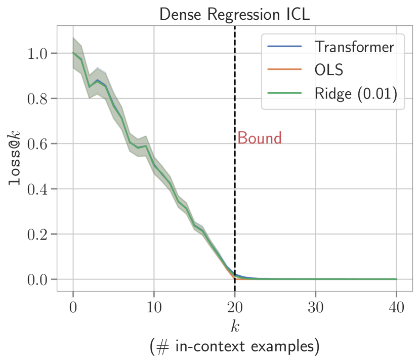
((a))

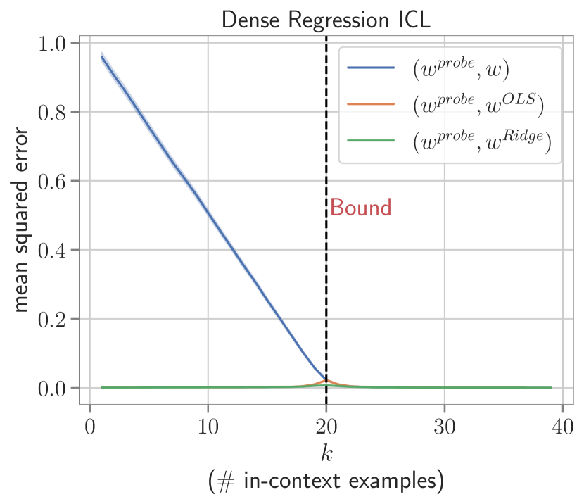
((b))

Figure 8: Results on the Dense Regression tasks mentioned in section §3.1.1.

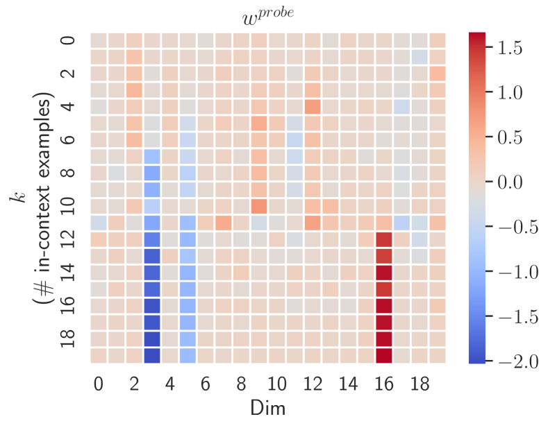
((a))

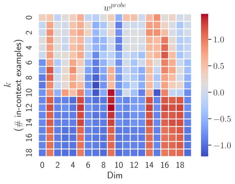
((b))

Figure 10: Visualizing recovered weights for sparse and sign vector regression for one of the examples in the test set.

A.5 Fourier Series Detailed results

In §3.2.1 and Figures 2(b) and 2(c), we could only discuss results for a subset of values of $M$ and $k$. The function visualizations for the transformer and Fourier OLS baseline for different combinations of $M$ and $k$ are provided in Figure 12. We have observations consistent with Figure 2(b), where the function outputs of the transformer and the baseline align closely. Similarly, in Figure 11, we present the distribution of frequencies in the predicted functions for the two methods and again observe consistent findings.

Figure 11: Measuring the frequencies of the simulated function by the transformer and the baseline for different values of $M$ (maximum frequency) and $k$ (number of in-context examples)

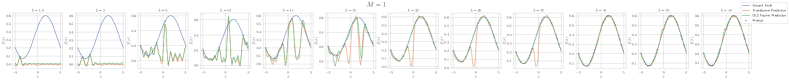
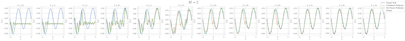
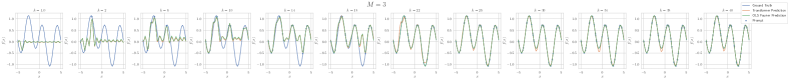
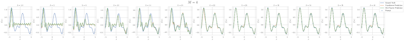
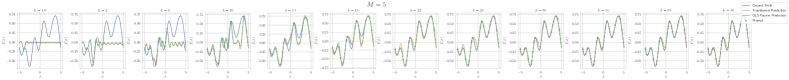
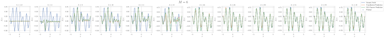
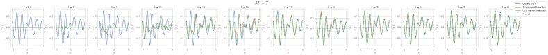
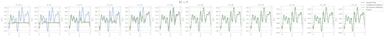
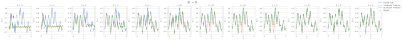
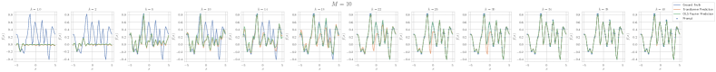
Figure 12: Visualizing the functions simulated by the transformer and the OLS Fourier Basis, for different values of $M$ (maximum frequency) and $k$ (number of in-context examples)

A.6 Degree-2 Monomial Basis Regression

We now detail the degree-2 monomial basis regression function family that was mentioned in §3.2.3. As stated in §3.2.1, the Fourier Series function class can be viewed as linear regression over the Fourier basis consisting of sinusoidal functions. Similarly, we define a function class $\mathcal{F}_{\Phi_{M}}^{\text{mon.(2)}}$ with the basis formed by degree-2 monomials for any $d$-dimensional input vector $\bm{\mathit{x}}$.

Using the notation introduced in 3.1.1 the basis for $\mathcal{F}_{\Phi_{M}}^{\text{mon.(2)}}$ is defined as $\Phi_{M}(\bm{\mathit{x}})=\{x_{i}x_{j}\ |\ 1\leq i,j\leq d\}$. Each function $f\in\mathcal{F}_{\Phi_{M}}^{\text{mon.(2)}}$ is a linear combination of basis and $\bm{\mathit{w}}$ i.e. $f(\bm{\mathit{x}})=\bm{\mathit{w}}^{T}\Phi_{M}(\bm{\mathit{x}})$, where $\bm{\mathit{w}}$ is a $|\Phi_{M}|$-dimensional vector sampled from standard normal distribution.

For experimentation, we define a sub-family $\mathcal{F}_{\mathcal{S}}^{\text{mon.(2)}}$ under $\mathcal{F}_{\Phi_{M}}^{\text{mon.(2)}}$ by choosing a proper subset $\mathcal{S}\subset\Phi_{M}$ and linearly combining the terms in $\mathcal{S}$ to form $f$. This is equivalent to explicitly setting coefficients $w_{i}$ of terms in $\Phi_{M}-\mathcal{S}$ to 0. We experiment with $d=20$, with the prompt length $p=290$ and $|\mathcal{S}|=20$. We do not use curriculum ($d,p,|\mathcal{S}|$ are fixed for the entire duration of the training run).

Baselines. We use OLS fitted to the following bases as baselines: $\mathcal{S}$ basis ($\text{OLS}_{\mathcal{S}}$), all degree-2 monomials i.e., $\Phi_{M}$ basis ($\text{OLS}_{\Phi_{M}}$), and to a basis of all polynomial features up to degree-2 ($\text{OLS}_{\text{poly.(2)}}$). We also compare Lasso ($\alpha=0.01$) fitted to all degree-2 monomials i.e., $\Phi_{M}$ basis ($\text{Lasso}_{\Phi_{M}}$) as a baseline.

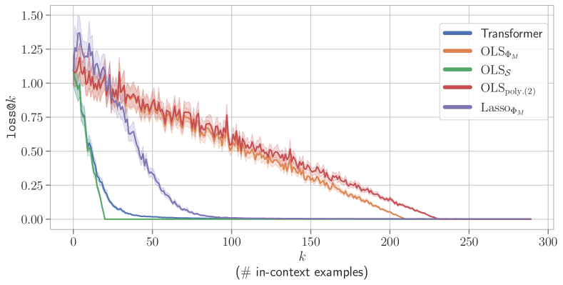
Figure 13: In-Distribution evaluation results on $\mathcal{F}_{\mathcal{S}}^{\text{mon.(2)}}$ sub-family of degree-2 monomial basis regression. Evaluation of transformer on prompts generated using the same $\mathcal{S}$ used during training.

((a))

((b))

((c))

((d))

((e))

((f))

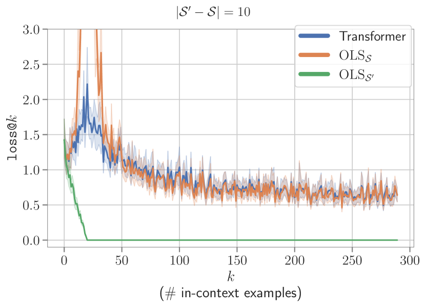
((g))

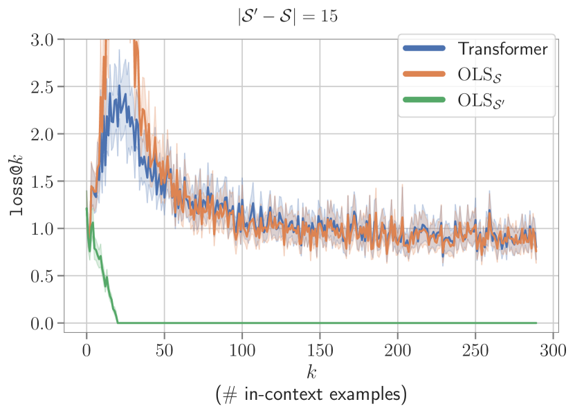
((h))

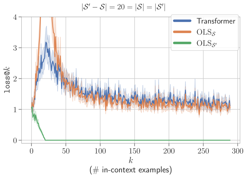
((i))

Figure 14: Out-of-Distribution evaluation results on $\mathcal{F}_{\mathcal{S}}^{\text{mon.(2)}}$ sub-family of degree-2 monomial basis regression. Evaluation of transformer trained on prompts generated using $\mathcal{S}^{\prime}$, where $\mathcal{S}^{\prime}$ contains $n$ degree-2 monomials not present in $\mathcal{S}$ that was used during training. We show results for different values of $n$.

Results. In Figure 13, we show the In-Distribution (ID) evaluation results for the $\mathcal{F}_{\mathcal{S}}^{\text{mon.(2)}}$ experiments. Here, the test prompts contain functions formed by $\mathcal{S}$ (the same basis used during training). We observe that Transformers closely follow $\text{OLS}_{\mathcal{S}}$. The increasing order of performance (decreasing $\texttt{loss@}k$ for $k\geq|\mathcal{S}|$) of different solvers is: $\text{OLS}_{\text{poly.(2)}}$ $\leq$ $\text{OLS}_{\Phi_{M}}$ $<$ $\text{Lasso}_{\Phi_{M}}$$<$ Transformers $<$ $\text{OLS}_{\mathcal{S}}$. Transformer’s squared error takes a little longer than $\text{OLS}_{\mathcal{S}}$  to converge. $\text{Lasso}_{\Phi_{M}}$  is able to take the advantage of sparsity of the problem and is hence better than both $\text{OLS}_{\Phi_{M}}$  and $\text{OLS}_{\text{poly.(2)}}$, which respectively converge at $k=210$ and $k=231$. We also conduct an Out-of-Distribution (OOD) evaluation for $\mathcal{F}_{\mathcal{S}}^{\text{mon.(2)}}$, whose results are shown in Figure 14. Here, we generate prompts from a basis $\mathcal{S}^{\prime}\subset\Phi_{M}$ of the same size as $\mathcal{S}$ but differing from $\mathcal{S}$ in $n$ degree-2 terms, i.e. $|\mathcal{S}^{\prime}-\mathcal{S}|=n$. We show the results for different values of $n$. Figure 14(a) shows the $\text{OLS}_{\mathcal{S}}$  undergoes a steep rise in errors momentarily at $k=|\mathcal{S}|$ (double descent). Figure 14(b) zooms into the lower error region of Figure 14(a) where we notice that Transformer mimics $\text{OLS}_{\mathcal{S}}$, while $\text{OLS}_{\mathcal{S}^{\prime}}$  is the best-performing baseline (since it fits to the $\mathcal{S}^{\prime}$ basis used to construct the prompts). Transformer does not undergo double descent (for $n=1$) and is hence momentarily better than $\text{OLS}_{\mathcal{S}}$  at $k=|\mathcal{S}|$. Similar plots are shown for $n\in\{2,3,4,5,10,15,20\}$. As $n$ increases, the height of $\text{OLS}_{\mathcal{S}}$  peak increases and the Transformer also starts to have a rise in errors at $k=|\mathcal{S}|$. For $n=20$, $\mathcal{S}^{\prime}$ and $\mathcal{S}$ have nothing in common, and Transformer still follows $\text{OLS}_{\mathcal{S}}$  (OLS fitted to the training basis $\mathcal{S}$). As mentioned under §3.2, when the prior on weights $\bm{\mathit{w}}$ is Gaussian, the PME is the minimum $L_{2}$-norm solution. For $\mathcal{F}_{\mathcal{S}}^{\text{mon.(2)}}$, that solution is given by $\text{OLS}_{\mathcal{S}}$. Therefore, the results suggest that the transformer is computing PME. In summary, transformers closely follow $\text{OLS}_{\mathcal{S}}$  in this set-up, and more so on the OOD data, where they even surpass $\text{OLS}_{\mathcal{S}}$’s  performance when it experiences double descent.

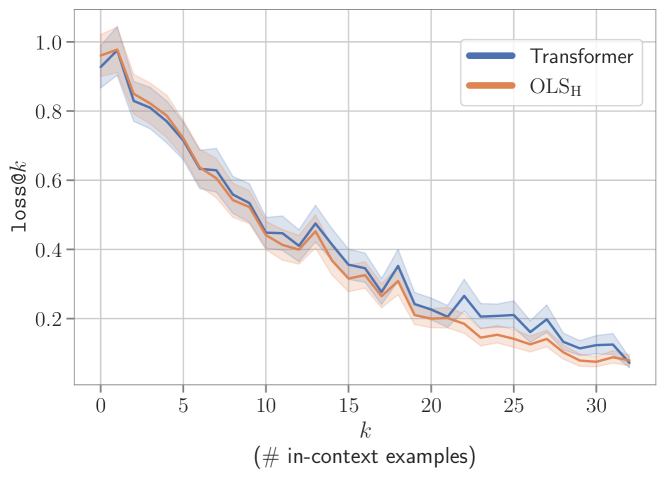
Figure 15: Evaluating Transformer trained on Haar Wavelet Basis Regression task ($\mathcal{F}_{\Phi_{H}}^{\text{Haar}}$).

A.7 Haar Wavelet Basis Regression

Similar to Fourier Series and Degree-2 Monomial Basis Regression, we also define another non-linear regression function family ($\mathcal{F}_{\Phi_{H}}^{\text{Haar}}$) using a different basis, $\Phi_{H}$, called the Haar wavelet basis. $\Phi_{H}$ is defined on the interval $[0,1]$ and is given by:

$$\Phi_{H}(x) =\{x\in[0,1]\mapsto\psi_{n,k}(x):n\in\mathbb{N}\cup\{0\},0\leq k<2^{n}\}\cup\{\mathbf{1}\},$$

$$\psi_{n,k}(x) =2^{n/2}\psi(2^{n}x-k),x\in[0,1],$$

$$\psi(x) =\begin{cases}1&0\leq x<\frac{1}{2},\\ -1&\frac{1}{2}\leq x<1,\\ 0&\mathrm{otherwise.}\end{cases}$$

, where ${\mathbf{1}}$ is the constant function which is $1$ everywhere on $[0,1]$. To define $f$, we sample $\bm{\mathit{w}}$ from $\mathcal{N}(0,1)$ and compute its dot product with the basis, i.e. $\bm{\mathit{w}}^{T}\Phi_{H}(\cdot)$. We construct the prompt $P$ by evaluating $f$ at different values of $\bm{\mathit{x}}\sim\mathcal{U}(0,1)$. The Transformer model is then trained on these prompts $P$.

We use $d=1$ and $p=32$, both of which are fixed throughout the training run, i.e. we do not use curriculum. We only consider the basis terms corresponding to $n\in\{0,1,2,3\}$. The baseline used is OLS on Haar Wavelet Basis features ($\text{OLS}_{\mathrm{H}}$). Note that for the model used throughout the paper (§2.1), at $k=32$ the $\texttt{loss@}k$ value is $0.18$, while for a bigger model and $\text{OLS}_{\mathrm{H}}$ it is $0.07$. Therefore, for this task we report the results for the bigger model which has 24 layers, 16 heads and 512 hidden size.

Results. In Figure 15, we observe that Transformer very closely mimics the errors of $\text{OLS}_{\mathrm{H}}$ (i.e. OLS fitted to the Haar Wavelet Basis) and converged to $\text{OLS}_{\mathrm{H}}$ at $k=32$. Since the prior on the weights $\bm{\mathit{w}}$ is Gaussian, $\text{OLS}_{\mathrm{H}}$ is the PME. Hence, Transformer’s performance on this task also suggests that it is simulating PME.

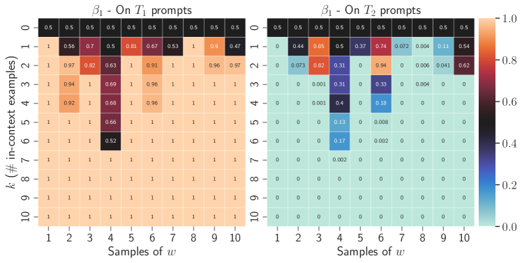
((a))

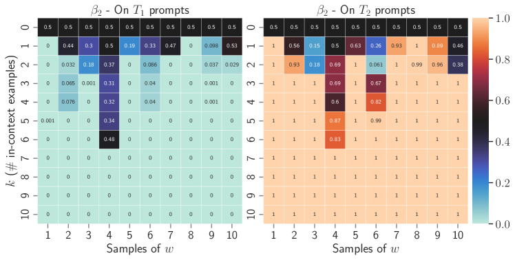
((b))

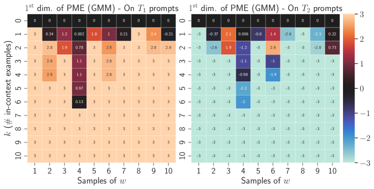
((c))

Figure 16: Evolution (as heatmaps) with prompt length ($k$) of $\beta$’s and PME (GMM) appearing in Eq. 4 for the model trained with $d=10,p=10,\alpha_{1}=\alpha_{2}=\frac{1}{2}$. We show $10$ different samples of $\bm{\mathit{w}}$ for each plot.

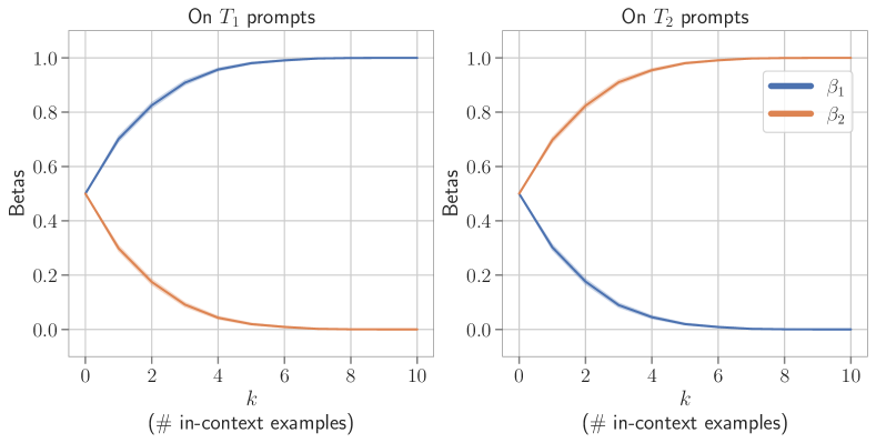
((a))

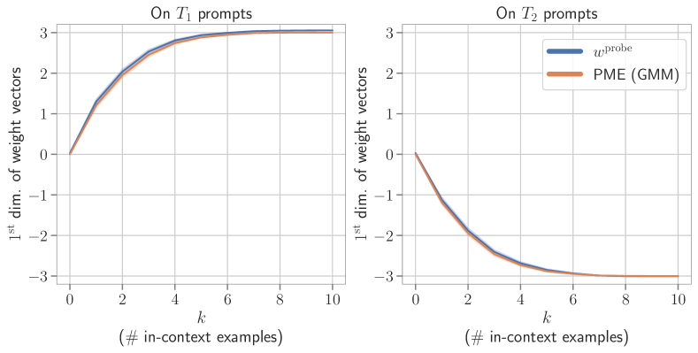
((b))

Figure 17: Evolution (as line plots) with prompt length ($k$) of $\beta$’s, PME (GMM), and $\bm{\mathit{w}}^{\mathrm{probe}}$ for the model trained with $d=10,p=10,\alpha_{1}=\alpha_{2}=\frac{1}{2}$. We show the values averaged over $1280$ samples.

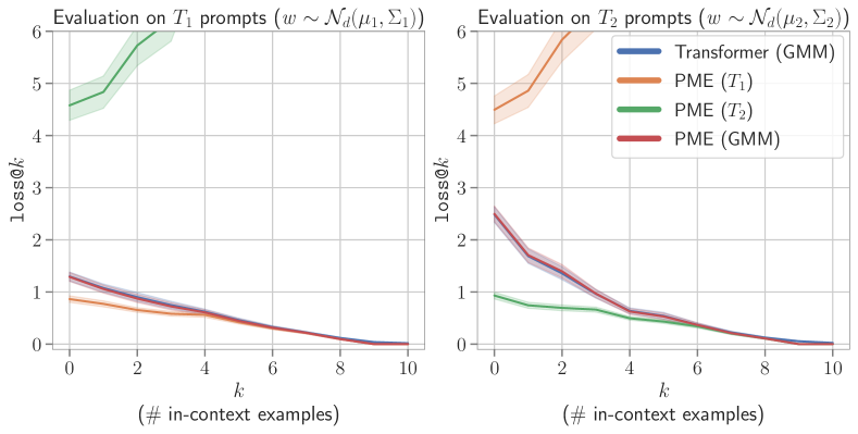
((a))

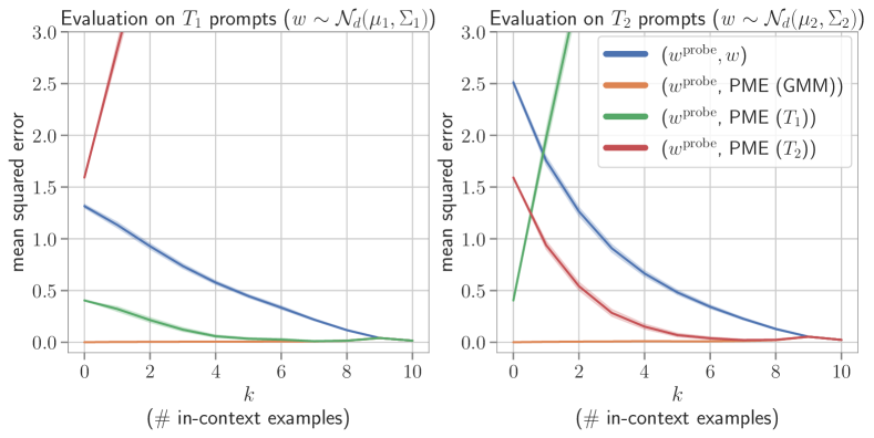
((b))

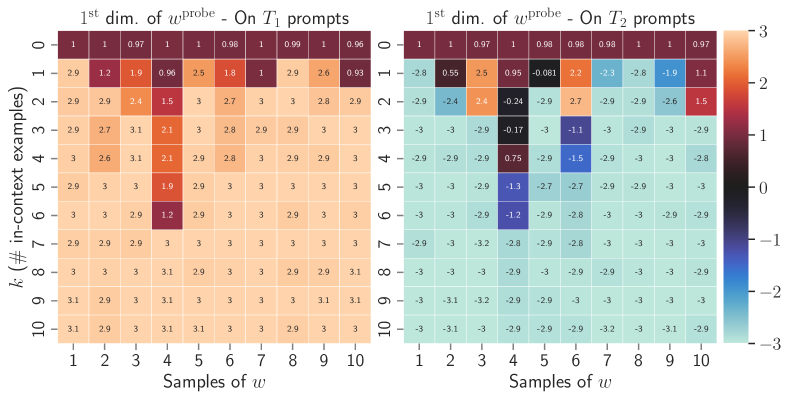
((c))

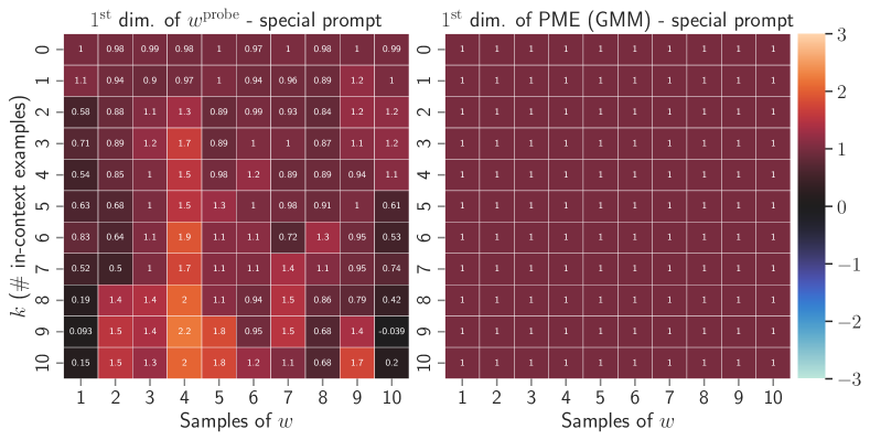
((d))

Figure 18: Transformers simulate PME when trained on dense regression task-mixture ($d=10,p=10,\alpha_{1}=\frac{2}{3},\alpha_{2}=\frac{1}{3}$) with weights having a mixture of Gaussian prior (GMM). (a): Comparing the performance of the Transformer with Posterior Mean Estimator (PME) of individual Gaussian components (PME ($T_{1}$) and PME ($T_{2}$)) and of the mixture PME (GMM). (b): MSE between the probed weights of the Transformer and PMEs. (c): $1^{\text{st}}$ dimension of Transformer’s probed weights across the prompt length. (d): $1^{\text{st}}$ dimension of Transformer’s probed weights and PME (GMM) across the prompt length for a specially constructed prompt.

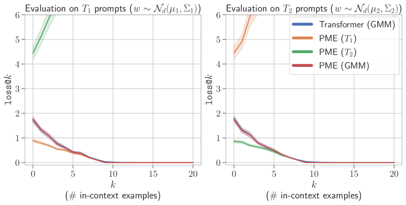
((a))

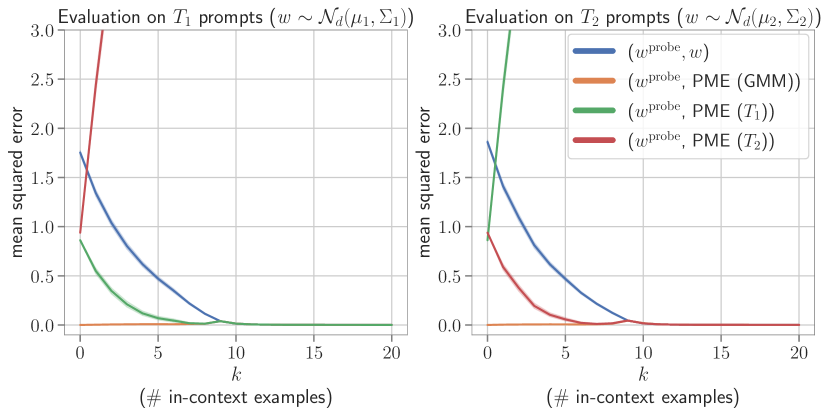
((b))

Figure 19: Transformers simulate PME when trained on dense regression task-mixture ($d=10,p=20,\alpha_{1}=\alpha 2=\frac{1}{2}$) with weights having a mixture of Gaussian prior (GMM). Left: Comparing the performance of the Transformer with Posterior Mean Estimator (PME) of individual Gaussian components (PME ($T_{1}$) and PME ($T_{2}$)) and of the mixture PME (GMM). Right: MSE between the probed weights of the Transformer and PMEs.

A.8 Gaussian Mixture Models (GMMs)

Here we discuss some details regarding §4.1 and more results on GMMs. We start with a description of how we calculate PMEs for this setup.

Computation of PMEs. As mentioned in §A.1 and §3.2, we can compute the individual PMEs for components $T_{1}$ and $T_{2}$ by minimizing the $L_{2}$ distance between the hyperplane induced by the prompt constraints and the mean of the Gaussian distribution. In particular, to compute PME for each Gaussian component of the prior, we solve a system of linear equations defined by the prompt constraints ($\bm{\mathit{w}}_{i}^{T}x_{i}=y_{i},\forall i\in\{1,2,..,p\}$) in conjunction with an additional constraint for the first coordinate, i.e. $(\bm{\mathit{w}})_{1}=+3$ (for $\mathcal{N}_{d}(\bm{\mu}_{1},\bm{\Sigma}_{1})$ or $\bm{\mathit{w}}_{1}=-3$ (for $\mathcal{N}_{d}(\bm{\mu}_{2},\bm{\Sigma}_{2})$). Given these individual PMEs, we calculate the PME of the mixture using Eq. 4.

Now we discuss more results for GMMs. First, we see the evolution of $\beta$’s (from Eq. 4), PME (GMM), and Transformer’s probed weights across the prompt length (Figures 16 and 17). Next, we see the results for the Transformer models trained on the mixture with unequal weights, i.e. $\alpha_{1}\neq\alpha_{2}$ (Figure 18) and for the $p=20$ model (Figure 19).

Evolution of $\beta$’s, PME (GMM), and $\bm{\mathit{w}}^{\mathrm{probe}}$. Figure 16 plots the evolution of $\beta$’s and $1^{\text{st}}$ dimension of PME (GMM) for $10$ different $\bm{\mathit{w}}$’s. The $\beta$’s (Figures 16(a) and 16(b)) are $0.5$ (equal to $\alpha$’s) at $k=0$ (when no information is observed from the prompt). Gradually, as more examples are observed from the prompt, $\beta_{T_{\mathrm{prompt}}}$ approaches $1$, while $\beta_{T_{\mathrm{other}}}$ approaches $0$. This is responsible for PME (GMM) converging to PME ($T_{\mathrm{prompt}}$) as seen in §4.1. The $1^{\mathrm{st}}$ dimension of PME (GMM) (Figure 16(c)) starts at $0$ and converges to $+3$ or $-3$ depending on whether $T_{\mathrm{prompt}}$  is $T_{1}$ or $T_{2}$. This is the same trend we saw for $\bm{\mathit{w}}^{\mathrm{probe}}$ in Figure 4(c). Figure 17 shows the same evolution in the form of line plots where we see the average across $1280$ samples of $\bm{\mathit{w}}$. In Figure 17(a), $\beta_{T_{\mathrm{prompt}}}$ approaches $1$, while $\beta_{T_{\mathrm{other}}}$ approaches $0$ as noted earlier. Consequently, in Figure 17(b), $1^{\mathrm{st}}$ dimension of PME (GMM) approaches $+3$ or $-3$ based on the prompt. The $1^{\mathrm{st}}$ dimension of Transformer’s probed weights, i.e. $(\bm{\mathit{w}}^{\mathrm{probe}})_{1}$  almost exactly mimics PME (GMM).

Unequal weight mixture with $\alpha_{1}=\frac{2}{3}\ \&\ \alpha_{2}=\frac{1}{3}$. Figure 18 shows the results for another model where $\alpha^{\prime}s$ are unequal ($d=10,p=10,\alpha_{1}=\frac{2}{3},\alpha_{2}=\frac{1}{3}$). The observations made for Figure 4 in §4.1 still hold true, with some notable aspects: (1) The difference between prediction errors, i.e. $\texttt{loss@}k$ (18(a)), of PME (GMM) and PME ($T_{1}$) is smaller than that of the uniform mixture ($\alpha_{1}=\alpha_{2}=\frac{1}{2}$) case, while the difference between prediction errors and weights of PME (GMM) and PME ($T_{2}$) is larger. This is because, at prompt length $=0$, PME (GMM) is a weighted combination of component PMEs with $\alpha$’s as coefficients (Eq. 4). Since $\alpha_{1}>\alpha_{2}$, PME (GMM) starts out as being closer to $T_{1}$ than $T_{2}$. Also, since the Transformer follows PME (GMM) throughout, its prediction errors also have similar differences (as PME (GMM)’s) with PMEs of both components $T_{1}$ and $T_{2}$. (2) Transformer’s probed weights ($\bm{\mathit{w}}^{\mathrm{probe}}$), which used to have the same MSE with PME ($T_{1}$) and PME ($T_{2}$) at $k=0$ in Figure 4(b), now give smaller MSE with PME ($T_{1}$) than PME ($T_{2}$) on prompts from both $T_{1}$ and $T_{2}$ (Figure 18(b)). This is a consequence of PME (GMM) starting out as being closer to $T_{1}$ than $T_{2}$ due to unequal mixture weights as discussed above. Since Transformer is simulating PME (GMM), $\bm{\mathit{w}}^{\mathrm{probe}}$ is also closer to PME ($T_{1}$) than PME ($T_{2}$) at $k=0$ regardless of which component ($T_{1}$ or $T_{2}$) the prompts come from. Due to $\bm{\mathit{w}}^{\mathrm{probe}}$ mimicking $T_{1}$ more than $T_{2}$ we also observe in Figure 18(b) that $\bm{\mathit{w}}^{\mathrm{probe}}$ gives smaller MSE with $\bm{\mathit{w}}$ (ground truth) when $T_{\mathrm{prompt}}$ = $T_{1}$ compared to when $T_{\mathrm{prompt}}$ = $T_{2}$. (3) The $1^{\text{st}}$ dimension of Transformer’s weights ($(\bm{\mathit{w}}^{\mathrm{probe}})_{1}$) and PME (GMM) is $1$ instead of $0$ (as in Figure 4(c)) when the prompt is either empty (18(c)) or lacks information regarding the distribution of $\bm{\mathit{w}}$ (18(d)). It happens because $(\bm{\mathit{w}}^{\mathrm{probe}})_{1}$ $\approx 1^{\text{st}}$ dimension of PME (GMM) $=(\bm{\mu}_{1})_{1}.\beta_{1}+(\bm{\mu}_{2})_{1}.\beta_{2}=(+3)(\frac{2}{3})+(-3)(\frac{1}{3})=1$. Note that $\beta_{1}=\alpha_{1}=\frac{2}{3}$ and $\beta_{2}=\alpha_{2}=\frac{1}{3}$ when prompt $P$ is empty at $k=0$ (Eq. 4). When $P$ is inconclusive of $\bm{\mathit{w}}$, $\beta_{1}=\alpha_{1}$ and $\beta_{2}=\alpha_{2}$ $\forall k\in\{1,2,\cdots,p\}$.

Transformer model trained with longer prompt length ($p=20$). Figure 19 depicts similar evidence as Figure 4 of Transformer simulating PME (GMM) for a model trained with $d=10,p=20,\alpha_{1}=\alpha_{2}=\frac{1}{2}$. We see that all the observations discussed in §4.1 also hold true for this model. Transformer converges to PME (GMM) and PME ($T_{\mathrm{prompt}}$) w.r.t. both $\texttt{loss@}k$ (Figure 19(a)) and weights (Figure 19(b)) at $k=10$ and keeps following them for larger $k$ as well.

In summary, all the evidence strongly suggests that Transformer performs Bayesian Inference and computes PME corresponding to the task at hand. If the task is a mixture, Transformer simulates the PME of the task mixture as given by 4.

A.9 ICL on task mixtures

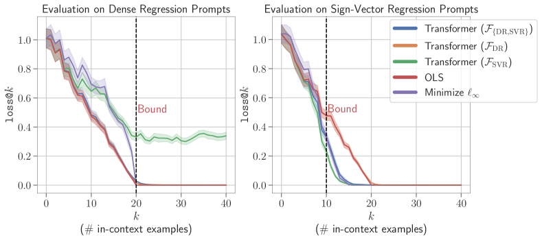
((a))

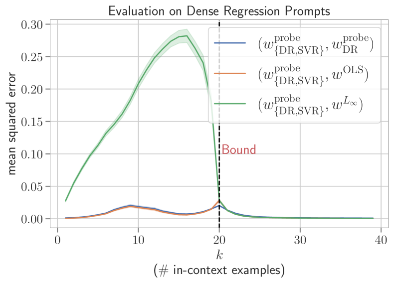
((b))

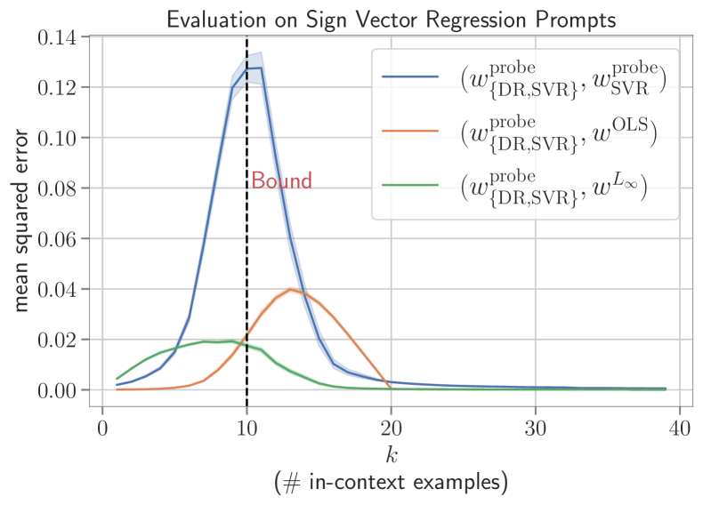
((c))

Figure 20: Comparing the performance of a Transformer model trained on dense and sign-vector regression mixture $\mathcal{F}_{\{\text{DR, SVR}\}}$ with baselines, as well as single task models, trained on $\mathcal{F}_{\text{DR}}$ and $\mathcal{F}_{\text{SVR}}$ individually. Top: Comparing $\texttt{loss@}k$ values of the mixture model with single-task models with different prompt distributions. Bottom: Comparing the errors between the weights recovered from the mixture model and different single task models and baselines while evaluating on $\mathcal{F}_{\text{DR}}$ and $\mathcal{F}_{\text{SVR}}$ prompts.

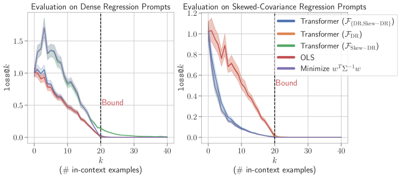
((a))

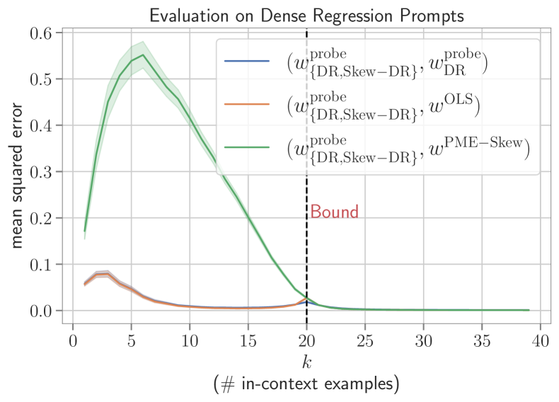
((b))

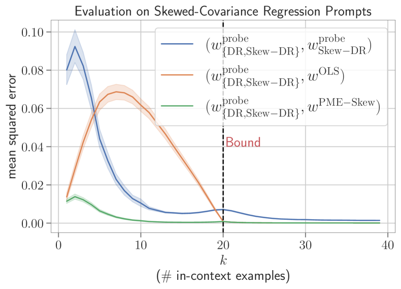
((c))

Figure 21: Comparing the performance of a Transformer model trained on dense and skewed-covariance regression mixture $\mathcal{F}_{\{\text{DR, Skew-DR}\}}$ with baselines, as well as single task models, trained on $\mathcal{F}_{\text{DR}}$ and $\mathcal{F}_{\text{Skew-DR}}$ individually. Top: Comparing $\texttt{loss@}k$ values of the mixture model with single-task models with different prompt distributions. Red (OLS) and orange (Transformer ($\mathcal{F}_{\text{DR}}$)) curves overlap very closely, so are a bit hard to distinguish in the plots. Similarly in the top right plot, purple (Minimize $\bm{\mathit{w}}^{T}\bm{\Sigma}^{-1}\bm{\mathit{w}}$) and green (Transformer $\mathcal{F}_{\text{Skew-DR}}$) curves overlap. Bottom: Comparing the errors between the weights recovered from the mixture model and different single task models and baselines while evaluating on $\mathcal{F}_{\text{DR}}$ and $\mathcal{F}_{\text{Skew-DR}}$ prompts.

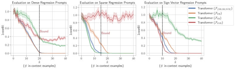
Figure 22: Comparing the performance of transformer model trained to in-context learn $\mathcal{F}_{\{\text{DR, SR, SVR}\}}$ mixture family with the corresponding single task models.

Here we detail some of the experiments with task mixtures that we discuss in passing in §4.2. Particularly, we describe the results for the homogeneous mixtures $\mathcal{F}_{\{\text{DR, SVR}\}}$, $\mathcal{F}_{\{\text{DR, Skew-DR}\}}$ and $\mathcal{F}_{\{\text{DR, SR, SVR}\}}$, as well as heterogeneous mixtures $\mathcal{F}_{\{\text{DR, DT}\}}$ and $\mathcal{F}_{\{\text{DT, NN}\}}$. As can be seen in Figure 20, the transformer model trained on $\mathcal{F}_{\{\text{DR, SVR}\}}$ mixture, behaves close to OLS when prompted with $f\in\mathcal{F}_{\text{DR}}$ and close to the $L_{\infty}$ minimization baseline when provided sign-vector regression prompts ($f\in\mathcal{F}_{\text{SVR}}$). We also have similar observations for the $\mathcal{F}_{\{\text{DR, Skew-DR}\}}$ mixture case in Figure 21, where the multi-task ICL model follows the PME of both tasks when sufficient examples are provided from the respective task. Similarly, for the model trained on the tertiary mixture $\mathcal{F}_{\{\text{DR, SR, SVR}\}}$ (as can be seen in Figure 22), the multi-task model can simulate the behavior of the three single-task models depending on the distribution of in-context examples. On $\mathcal{F}_{\text{SR}}$ and $\mathcal{F}_{\text{SVR}}$ prompts the multi-task model performs slightly worse compared to the single-task models trained on $\mathcal{F}_{\text{SR}}$ and $\mathcal{F}_{\text{SVR}}$ respectively, however once sufficient examples are provided (still $<20$), they do obtain close errors. This observation is consistent with the PME hypothesis i.e. once more evidence is observed the $\beta$ values PME of the mixture should converge to the PME of the task from which prompt $P$ is sampled. The results on heterogeneous mixtures we discuss in detail below:

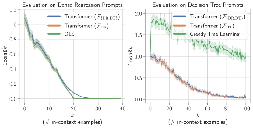
((a))

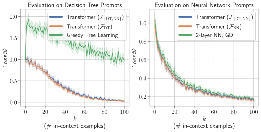
((b))

Figure 23: Multi-task in-context learning for heterogeneous mixtures.

Heterogeneous Mixtures: Up until now, our experiments for the multi-task case have been focused on task mixtures where all function families have the same parameterized form i.e $w^{T}x$ for linear mixtures and $w^{T}\Phi(x)$ for Fourier mixtures. We now move to more complex mixtures where this no longer holds true. In particular, we consider dense regression and decision tree mixture $\mathcal{F}_{\{\text{DR, DT}\}}$ and decision tree and neural network mixture $\mathcal{F}_{\{\text{DT, NN}\}}$.

We follow Garg et al. [2022]’s setup for decision trees and neural networks. We consider decision trees of depth 4 and 20-dimensional input vectors $\bm{\mathit{x}}$. A decision tree is sampled by choosing the split node randomly from the features at each depth, and the output of the function is given by the values stored in the leaf nodes which are sampled from $\mathcal{N}(0,1)$. For neural networks, we consider 2-layer (1 hidden + 1 output) multi-layer perceptrons (MLP) with ReLU non-linearity i.e. $f(x)=\sum_{i=1}^{r}\alpha_{i}\texttt{ReLU}(w_{i}^{T}\bm{\mathit{x}})$, where $\alpha\in\mathbb{R}$ and $\bm{\mathit{w}}_{i}\in\mathbb{R}^{d}$. The network parameters $a_{i}$s and $\bm{\mathit{w}}_{i}$s are sampled from $\mathcal{N}(0,2/r)$ and $\mathcal{N}(0,1)$ respectively. The input vectors $\bm{\mathit{x}}_{i}$s are sampled from $\mathcal{N}(0,1)$ for both tasks. We consider greedy tree learning and stochastic gradient descent over a 2-layer MLP as our baselines for decision trees and neural networks respectively. The values of hyperparameters for baselines such as the number of gradient descent steps, initial learning rate for Adam, etc. are the same as Garg et al. [2022].

The results for the two mixtures are provided in Figure 23. The mixture model Transformer ($\mathcal{F}_{\{\text{DR, DT}\}}$) follows the single task model Transformer ($\mathcal{F}_{\text{DR}}$) when provided in-context examples from $f\sim\mathcal{F}_{\text{DR}}$ and agrees with Transformer ($\mathcal{F}_{\text{DT}}$) when prompted with $f\sim\mathcal{F}_{\text{DT}}$ (Figure 23(a). Similarly, we have consistent findings for $\mathcal{F}_{\{\text{DT, NN}\}}$ mixture as well, where the model learns to solve both tasks depending upon the input prompt (Figure 23(b)).

A.10 Fourier series mixture detailed results

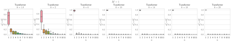
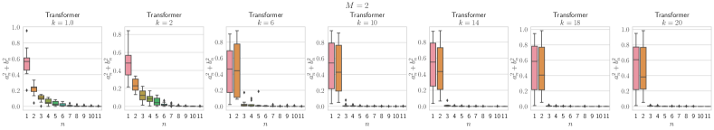
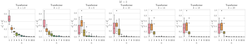
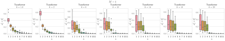
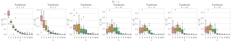
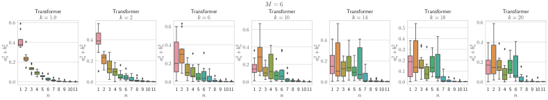
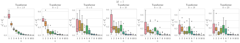
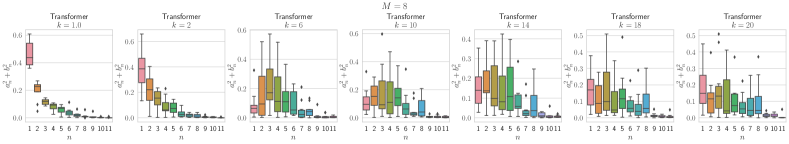
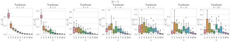
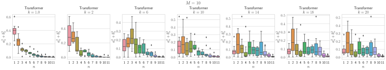
Figure 24: In-context learning of Fourier series mixture class. Measuring the frequencies of the simulated function by the transformer for different values of $M$ (maximum frequency) and $k$ (number of in-context examples). Showcases the simplicity bias behavior exhibited by the model at low frequencies.

In §4.3 we discussed results on $\mathcal{F}_{\Phi_{1:N}}^{\text{fourier}}$ mixture, where we showed visualizations of the inductive biases for $M=4$ and $M=10$, and $k=2$ and $k=20$. Here we confirm the observations from §4.3 by detailing results for different combinations of $M$ and $k$ in Figure 24. The findings are consistent with Figure 6(b), where for all values of $M$ we observe a case of simplicity bias towards low frequencies at smaller prompt lengths and as more examples are provided it is able to recognize the gold frequencies.

A.11 Conditions necessary for multi-task ICL

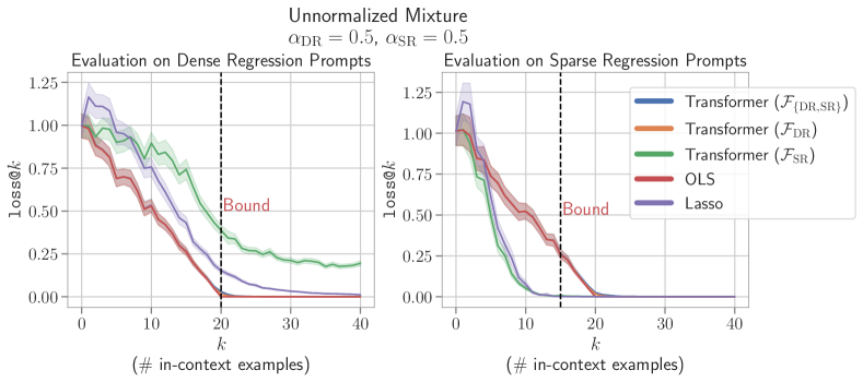
((a))

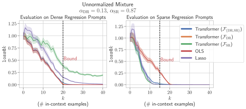
((b))

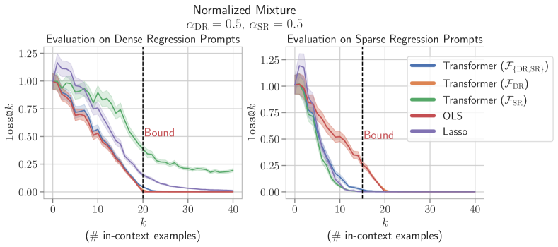
((c))

Figure 25: Conditions affecting multi-task ICL in transformers. Top: Evaluating $\texttt{loss@}k$ for transformer model trained on $\mathcal{F}_{\{\text{DR, SR}\}}$ task family without normalization and considering uniform mixtures (i.e. $\alpha_{\text{DR}}=\alpha_{\text{SR}}=0.5$), and comparing with single-task models and baselines. While the blue curve (Transformer $\mathcal{F}_{\{\text{DR, SR}\}}$) is hard to see here, it is because it overlaps almost perfectly with the red curve corresponding to OLS in both cases.Center: Similar plots as above but for the model trained on the mixture $\mathcal{F}_{\{\text{DR, SR}\}}$ with non-uniform weights i.e. $\alpha_{\text{DR}}=0.13,\alpha_{\text{SR}}=0.87$. Bottom: Training the model with the normalized (and uniform) mixture such that outputs for the two tasks have the same variance. All the models are trained with the curriculum. The discussion continues in Figure 26 for the models trained without curriculum.

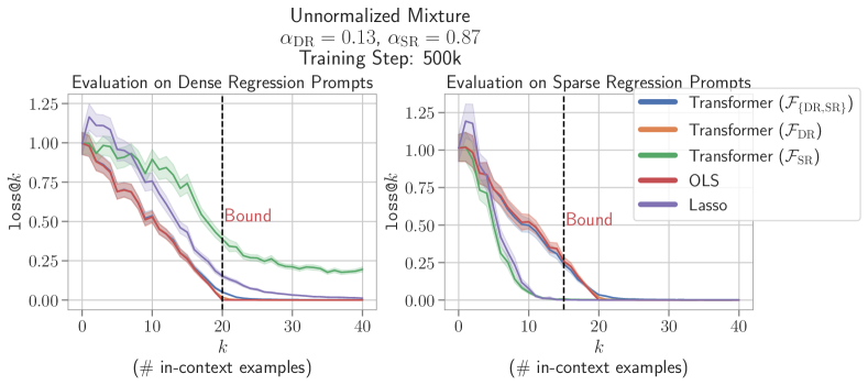
((a))

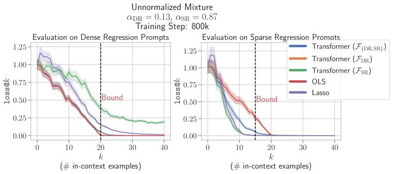
((b))

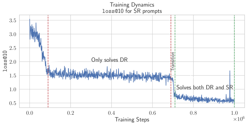
((c))

Figure 26: Evaluating transformer model trained without curriculum on $\mathcal{F}_{\{\text{DR, SR}\}}$ task family without normalization and non-uniform weights i.e. $\alpha_{\text{DR}}=0.13,\alpha_{\text{SR}}=0.87$ (similar to Figure 25(b)). Top: Evaluating the checkpoint corresponding to the 500k training step of the aforementioned model. Again, the blue curve (Transformer $\mathcal{F}_{\{\text{DR, SR}\}}$) is hard to see here, but it is because it overlaps almost perfectly with the red curve corresponding to OLS in both cases.Center: Evaluating the same model but a much later checkpoint i.e. at 800k training step. Bottom: Evolution of $\texttt{loss@}10$ on $\mathcal{F}_{\text{SR}}$ prompts while training the above model.

We detail the results for conditions affecting multi-task ICL discussed in §4.2 here. Figure 25 compares transformer models trained on $\mathcal{F}_{\{\text{DR, SR}\}}$ mixture with different setups i.e. training without task-normalization and uniform mixture weights $\alpha_{i}$’s (Figure 25(a)), training without task-normalization and non-uniform mixture weights (Figure 25(b)), and training with task normalization and uniform mixture weights (Figure 25(c)). As described in §4.2, we perform task normalization by ensuring that the outputs $f(x)$ for all the tasks have the same variance, which results in all the tasks providing a similar training signal to the model. To perform normalization, we simply divide the weights $w$ sampled for the tasks by a normalization constant, which is decided according to the nature of the task. With this, we make sure that the output $y=w^{T}x$ has a unit variance. The normalization constants for different tasks are provided in Table 2.

Table 2: Normalization constants used for different tasks to define normalized mixtures for multi-task ICL experiments. Here $d$ denotes the size of the weight vectors used in linear-inverse problems as well as the last layer of the neural network. $s$ refers to the sparsity of sparse regression problems, $r$ is the hidden size of the neural network and $N$ refers to the maximum frequency for Fourier series.

Function Family	Normalization Constant
Dense Regression	$\sqrt{d}$
Sparse Regression	$\sqrt{s}$
Sign-Vector Regression	$\sqrt{d}$
Fourier-Series	$N$
Degree-2 Monomial Basis Regression	$\sqrt{|\mathcal{S}|}$
Decision Trees	1
Neural Networks	$\sqrt{\frac{dr}{2}}$

All the experiments discussed above (like most others in the main paper) were performed using curriculum learning. As discussed in §4.2, we investigated if the curriculum has any effect on multi-task ICL capabilities. The results for the same are provided in Figure 26.

We also explore the effect of normalization on multi-task ICL in Figure 27 for $\mathcal{F}_{\{\text{DR, SVR}\}}$ task. As can be seen in Figure 27(a), for this particular mixture even while training the model without normalization, the model exhibited multi-task ICL, which can be explained by both tasks having the same output variance (i.e. $d$). Interestingly, when we evaluate this model (i.e. the one trained on unnormalized mixture) on in-context examples which have the outputs $f(x_{i})$’s normalized, the model fails to solve $\mathcal{F}_{\text{SVR}}$ and follows OLS baseline for both the tasks. We hypothesize that since this situation represents Out of Distribution (OOD) evaluation and the model might not be robust towards performing multi-task ICL on prompts that come from a different distribution than those seen during training. Exploring OOD generalization in the multi-task case is a compelling direction that we leave for future work.

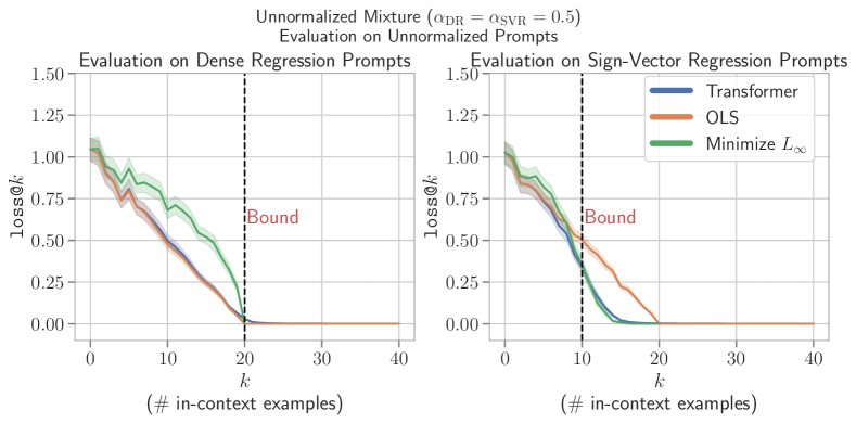
((a))

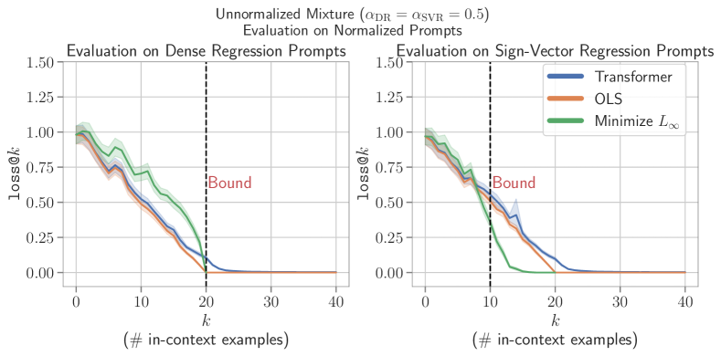
((b))

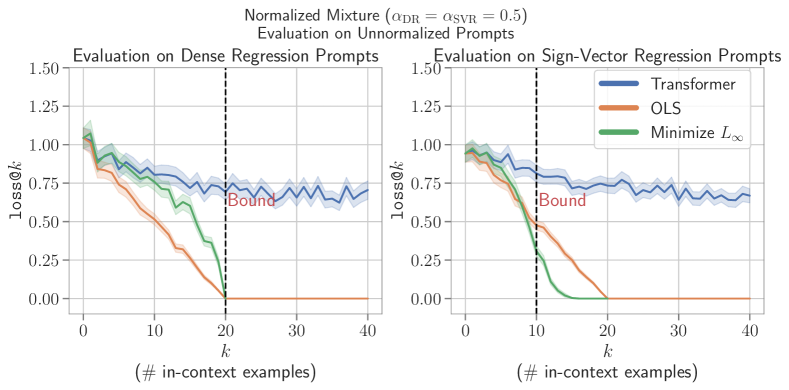
((c))

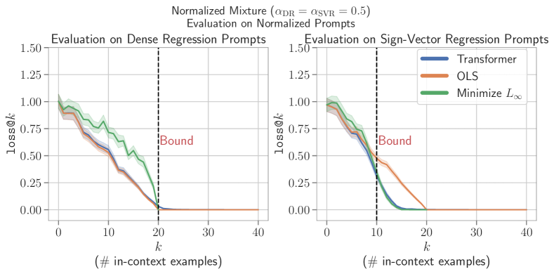
((d))

Figure 27: Effect of output normalization on multi-task ICL in transformers. Top Left (a): A transformer model is trained on a uniform mixture of $\mathcal{F}_{\{\text{DR, SVR}\}}$ task family (i.e. $\alpha_{\text{DR}}=\alpha_{\text{SVR}}=0.5$) without normalization. Evaluating $\texttt{loss@}k$ for this model on unnormalized prompts (where outputs $f(x)$ are not normalized to have unit variance i.e. same as training). Note that for the $\mathcal{F}_{\{\text{DR, SVR}\}}$ task family even without normalization the outputs $f(x)$ have the same mean and variance ($\mu=0,\sigma^{2}=20$) for both the tasks. Bottom Left (b): Evaluating $\texttt{loss@}k$ for the model in (a) on normalized prompts (where outputs $f(x)$ for both tasks are normalized to have unit variance). Top Right (c): A transformer model is trained on a uniform mixture of $\mathcal{F}_{\{\text{DR, SVR}\}}$ task family (i.e. $\alpha_{\text{DR}}=\alpha_{\text{SVR}}=0.5$) with normalization. Evaluating $\texttt{loss@}k$ for this model on unnormalized prompts. Bottom Right (d) Evaluating $\texttt{loss@}k$ for the model in (c) on normalized prompts. All the models are trained with the curriculum.

References

- Akyürek et al. [2022] Ekin Akyürek, Dale Schuurmans, Jacob Andreas, Tengyu Ma, and Denny Zhou. What learning algorithm is in-context learning? investigations with linear models. CoRR, abs/2211.15661, 2022. doi: 10.48550/arXiv.2211.15661. URL https://doi.org/10.48550/arXiv.2211.15661.
- Bhattamishra et al. [2020] Satwik Bhattamishra, Kabir Ahuja, and Navin Goyal. On the Ability and Limitations of Transformers to Recognize Formal Languages. In Proceedings of the 2020 Conference on Empirical Methods in Natural Language Processing (EMNLP), pages 7096–7116, Online, November 2020. Association for Computational Linguistics. doi: 10.18653/v1/2020.emnlp-main.576. URL https://aclanthology.org/2020.emnlp-main.576.
- Bhattamishra et al. [2022] Satwik Bhattamishra, Arkil Patel, Varun Kanade, and Phil Blunsom. Simplicity bias in transformers and their ability to learn sparse boolean functions. 2022.
- Brown et al. [2020] Tom B. Brown, Benjamin Mann, Nick Ryder, Melanie Subbiah, Jared Kaplan, Prafulla Dhariwal, Arvind Neelakantan, Pranav Shyam, Girish Sastry, Amanda Askell, Sandhini Agarwal, Ariel Herbert-Voss, Gretchen Krueger, Tom Henighan, Rewon Child, Aditya Ramesh, Daniel M. Ziegler, Jeffrey Wu, Clemens Winter, Christopher Hesse, Mark Chen, Eric Sigler, Mateusz Litwin, Scott Gray, Benjamin Chess, Jack Clark, Christopher Berner, Sam McCandlish, Alec Radford, Ilya Sutskever, and Dario Amodei. Language models are few-shot learners. In Hugo Larochelle, Marc’Aurelio Ranzato, Raia Hadsell, Maria-Florina Balcan, and Hsuan-Tien Lin, editors, Advances in Neural Information Processing Systems 33: Annual Conference on Neural Information Processing Systems 2020, NeurIPS 2020, December 6-12, 2020, virtual, 2020. URL https://proceedings.neurips.cc/paper/2020/hash/1457c0d6bfcb4967418bfb8ac142f64a-Abstract.html.
- Canatar et al. [2021] A. Canatar, B. Bordelon, and C. Pehlevan. Spectral bias and task-model alignment explain generalization in kernel regression and infinitely wide neural networks. Nature Communications, 12, 2021.
- Chan et al. [2022a] Stephanie Chan, Adam Santoro, Andrew Lampinen, Jane Wang, Aaditya Singh, Pierre Richemond, James McClelland, and Felix Hill. Data distributional properties drive emergent in-context learning in transformers. In S. Koyejo, S. Mohamed, A. Agarwal, D. Belgrave, K. Cho, and A. Oh, editors, Advances in Neural Information Processing Systems, volume 35, pages 18878–18891. Curran Associates, Inc., 2022a. URL https://proceedings.neurips.cc/paper_files/paper/2022/file/77c6ccacfd9962e2307fc64680fc5ace-Paper-Conference.pdf.
- Chan et al. [2022b] Stephanie C. Y. Chan, Ishita Dasgupta, Junkyung Kim, Dharshan Kumaran, Andrew K. Lampinen, and Felix Hill. Transformers generalize differently from information stored in context vs in weights. CoRR, abs/2210.05675, 2022b. doi: 10.48550/arXiv.2210.05675. URL https://doi.org/10.48550/arXiv.2210.05675.
- Chandrasekaran et al. [2012] Venkat Chandrasekaran, Benjamin Recht, Pablo A. Parrilo, and Alan S. Willsky. The convex geometry of linear inverse problems. Foundations of Computational Mathematics, 12(6):805–849, oct 2012. doi: 10.1007/s10208-012-9135-7. URL https://doi.org/10.1007%2Fs10208-012-9135-7.
- Domingos [1999] Pedro M. Domingos. The role of occam’s razor in knowledge discovery. Data Min. Knowl. Discov., 3(4):409–425, 1999. doi: 10.1023/A:1009868929893. URL https://doi.org/10.1023/A:1009868929893.
- Dong et al. [2023] Qingxiu Dong, Lei Li, Damai Dai, Ce Zheng, Zhiyong Wu, Baobao Chang, Xu Sun, Jingjing Xu, Lei Li, and Zhifang Sui. A survey on in-context learning, 2023.
- Fridovich-Keil et al. [2022] Sara Fridovich-Keil, Raphael Gontijo Lopes, and Rebecca Roelofs. Spectral bias in practice: The role of function frequency in generalization. In NeurIPS, 2022. URL http://papers.nips.cc/paper_files/paper/2022/hash/306264db5698839230be3642aafc849c-Abstract-Conference.html.
- Garg et al. [2022] Shivam Garg, Dimitris Tsipras, Percy S Liang, and Gregory Valiant. What can transformers learn in-context? a case study of simple function classes. In S. Koyejo, S. Mohamed, A. Agarwal, D. Belgrave, K. Cho, and A. Oh, editors, Advances in Neural Information Processing Systems, volume 35, pages 30583–30598. Curran Associates, Inc., 2022. URL https://proceedings.neurips.cc/paper_files/paper/2022/file/c529dba08a146ea8d6cf715ae8930cbe-Paper-Conference.pdf.
- Goldblum et al. [2023] Micah Goldblum, Marc Finzi, Keefer Rowan, and Andrew Gordon Wilson. The no free lunch theorem, kolmogorov complexity, and the role of inductive biases in machine learning. CoRR, abs/2304.05366, 2023. doi: 10.48550/arXiv.2304.05366. URL https://doi.org/10.48550/arXiv.2304.05366.
- Hahn and Goyal [2023] Michael Hahn and Navin Goyal. A theory of emergent in-context learning as implicit structure induction. CoRR, abs/2303.07971, 2023. doi: 10.48550/arXiv.2303.07971. URL https://doi.org/10.48550/arXiv.2303.07971.
- Haviv et al. [2022] Adi Haviv, Ori Ram, Ofir Press, Peter Izsak, and Omer Levy. Transformer language models without positional encodings still learn positional information. In Findings of the Association for Computational Linguistics: EMNLP 2022, pages 1382–1390, Abu Dhabi, United Arab Emirates, December 2022. Association for Computational Linguistics. URL https://aclanthology.org/2022.findings-emnlp.99.
- Hoffmann et al. [2022] Jordan Hoffmann, Sebastian Borgeaud, Arthur Mensch, Elena Buchatskaya, Trevor Cai, Eliza Rutherford, Diego de Las Casas, Lisa Anne Hendricks, Johannes Welbl, Aidan Clark, Tom Hennigan, Eric Noland, Katie Millican, George van den Driessche, Bogdan Damoc, Aurelia Guy, Simon Osindero, Karen Simonyan, Erich Elsen, Jack W. Rae, Oriol Vinyals, and Laurent Sifre. Training compute-optimal large language models. 2022.
- Hospedales et al. [2022] T. Hospedales, A. Antoniou, P. Micaelli, and A. Storkey. Meta-learning in neural networks: A survey. IEEE Transactions on Pattern Analysis and Machine Intelligence, 44(09):5149–5169, sep 2022. ISSN 1939-3539. doi: 10.1109/TPAMI.2021.3079209.
- Kingma and Ba [2015] Diederik P. Kingma and Jimmy Ba. Adam: A method for stochastic optimization. In Yoshua Bengio and Yann LeCun, editors, 3rd International Conference on Learning Representations, ICLR 2015, San Diego, CA, USA, May 7-9, 2015, Conference Track Proceedings, 2015. URL http://arxiv.org/abs/1412.6980.
- Liu et al. [2023] Pengfei Liu, Weizhe Yuan, Jinlan Fu, Zhengbao Jiang, Hiroaki Hayashi, and Graham Neubig. Pre-train, prompt, and predict: A systematic survey of prompting methods in natural language processing. ACM Comput. Surv., 55(9):195:1–195:35, 2023. doi: 10.1145/3560815. URL https://doi.org/10.1145/3560815.
- Mangasarian and Recht [2011] O.L. Mangasarian and Benjamin Recht. Probability of unique integer solution to a system of linear equations. European Journal of Operational Research, 214(1):27–30, 2011. ISSN 0377-2217. doi: https://doi.org/10.1016/j.ejor.2011.04.010. URL https://www.sciencedirect.com/science/article/pii/S0377221711003511.
- Min et al. [2022a] Sewon Min, Mike Lewis, Luke Zettlemoyer, and Hannaneh Hajishirzi. MetaICL: Learning to learn in context. In Proceedings of the 2022 Conference of the North American Chapter of the Association for Computational Linguistics: Human Language Technologies, pages 2791–2809, Seattle, United States, July 2022a. Association for Computational Linguistics. doi: 10.18653/v1/2022.naacl-main.201. URL https://aclanthology.org/2022.naacl-main.201.
- Min et al. [2022b] Sewon Min, Xinxi Lyu, Ari Holtzman, Mikel Artetxe, Mike Lewis, Hannaneh Hajishirzi, and Luke Zettlemoyer. Rethinking the role of demonstrations: What makes in-context learning work? In Proceedings of the 2022 Conference on Empirical Methods in Natural Language Processing, pages 11048–11064, Abu Dhabi, United Arab Emirates, December 2022b. Association for Computational Linguistics. URL https://aclanthology.org/2022.emnlp-main.759.
- Mingard et al. [2023] Chris Mingard, Henry Rees, Guillermo Valle Pérez, and Ard A. Louis. Do deep neural networks have an inbuilt occam’s razor? CoRR, abs/2304.06670, 2023. doi: 10.48550/arXiv.2304.06670. URL https://doi.org/10.48550/arXiv.2304.06670.
- Mueller and Linzen [2023] Aaron Mueller and Tal Linzen. How to plant trees in language models: Data and architectural effects on the emergence of syntactic inductive biases. 2023.
- Olsson et al. [2022] Catherine Olsson, Nelson Elhage, Neel Nanda, Nicholas Joseph, Nova DasSarma, Tom Henighan, Ben Mann, Amanda Askell, Yuntao Bai, Anna Chen, Tom Conerly, Dawn Drain, Deep Ganguli, Zac Hatfield-Dodds, Danny Hernandez, Scott Johnston, Andy Jones, Jackson Kernion, Liane Lovitt, Kamal Ndousse, Dario Amodei, Tom Brown, Jack Clark, Jared Kaplan, Sam McCandlish, and Chris Olah. In-context learning and induction heads. Transformer Circuits Thread, 2022. https://transformer-circuits.pub/2022/in-context-learning-and-induction-heads/index.html.
- Pan et al. [2023] Jane Pan, Tianyu Gao, Howard Chen, and Danqi Chen. What in-context learning ”learns” in-context: Disentangling task recognition and task learning, 2023.
- Paszke et al. [2019] Adam Paszke, Sam Gross, Francisco Massa, Adam Lerer, James Bradbury, Gregory Chanan, Trevor Killeen, Zeming Lin, Natalia Gimelshein, Luca Antiga, Alban Desmaison, Andreas Kopf, Edward Yang, Zachary DeVito, Martin Raison, Alykhan Tejani, Sasank Chilamkurthy, Benoit Steiner, Lu Fang, Junjie Bai, and Soumith Chintala. Pytorch: An imperative style, high-performance deep learning library. In H. Wallach, H. Larochelle, A. Beygelzimer, F. d'Alché-Buc, E. Fox, and R. Garnett, editors, Advances in Neural Information Processing Systems, volume 32. Curran Associates, Inc., 2019. URL https://proceedings.neurips.cc/paper_files/paper/2019/file/bdbca288fee7f92f2bfa9f7012727740-Paper.pdf.
- Press et al. [2022] Ofir Press, Noah Smith, and Mike Lewis. Train short, test long: Attention with linear biases enables input length extrapolation. In International Conference on Learning Representations, 2022. URL https://openreview.net/forum?id=R8sQPpGCv0.
- Radford et al. [2019] Alec Radford, Jeffrey Wu, Rewon Child, David Luan, Dario Amodei, and Ilya Sutskever. Language models are unsupervised multitask learners. https://d4mucfpksywv.cloudfront.net/better-language-models/language-models.pdf, 1(8):9, 2019.
- Rahaman et al. [2019] Nasim Rahaman, Aristide Baratin, Devansh Arpit, Felix Draxler, Min Lin, Fred A. Hamprecht, Yoshua Bengio, and Aaron C. Courville. On the spectral bias of neural networks. In Kamalika Chaudhuri and Ruslan Salakhutdinov, editors, Proceedings of the 36th International Conference on Machine Learning, ICML 2019, 9-15 June 2019, Long Beach, California, USA, volume 97 of Proceedings of Machine Learning Research, pages 5301–5310. PMLR, 2019. URL http://proceedings.mlr.press/v97/rahaman19a.html.
- Rahimi and Recht [2007] Ali Rahimi and Benjamin Recht. Random features for large-scale kernel machines. In J. Platt, D. Koller, Y. Singer, and S. Roweis, editors, Advances in Neural Information Processing Systems, volume 20. Curran Associates, Inc., 2007. URL https://proceedings.neurips.cc/paper_files/paper/2007/file/013a006f03dbc5392effeb8f18fda755-Paper.pdf.
- Razeghi et al. [2022] Yasaman Razeghi, Robert L. Logan IV au2, Matt Gardner, and Sameer Singh. Impact of pretraining term frequencies on few-shot reasoning. 2022.
- Saunshi et al. [2021] Nikunj Saunshi, Sadhika Malladi, and Sanjeev Arora. A mathematical exploration of why language models help solve downstream tasks. In 9th International Conference on Learning Representations, ICLR 2021, Virtual Event, Austria, May 3-7, 2021. OpenReview.net, 2021. URL https://openreview.net/forum?id=vVjIW3sEc1s.
- Schmidhuber [1987] Jurgen Schmidhuber. Evolutionary principles in self-referential learning. on learning now to learn: The meta-meta-meta…-hook. Diploma thesis, Technische Universitat Munchen, Germany, 14 May 1987. URL http://www.idsia.ch/~juergen/diploma.html.
- Si et al. [2023] Chenglei Si, Dan Friedman, Nitish Joshi, Shi Feng, Danqi Chen, and He He. Measuring inductive biases of in-context learning with underspecified demonstrations, 2023.
- Su et al. [2021] Jianlin Su, Yu Lu, Shengfeng Pan, Bo Wen, and Yunfeng Liu. Roformer: Enhanced transformer with rotary position embedding. CoRR, abs/2104.09864, 2021. URL https://arxiv.org/abs/2104.09864.
- Thrun and Pratt [2012] Sebastian Thrun and Lorien Pratt, editors. Learning to Learn. Springer Science and Business Media, 2012.
- Tibshirani [1996] Robert Tibshirani. Regression shrinkage and selection via the lasso. Journal of the Royal Statistical Society: Series B (Methodological), 58(1):267–288, 1996. doi: https://doi.org/10.1111/j.2517-6161.1996.tb02080.x. URL https://rss.onlinelibrary.wiley.com/doi/abs/10.1111/j.2517-6161.1996.tb02080.x.
- Touvron et al. [2023] Hugo Touvron, Thibaut Lavril, Gautier Izacard, Xavier Martinet, Marie-Anne Lachaux, Timothée Lacroix, Baptiste Rozière, Naman Goyal, Eric Hambro, Faisal Azhar, Aurelien Rodriguez, Armand Joulin, Edouard Grave, and Guillaume Lample. Llama: Open and efficient foundation language models. 2023.
- Vaswani et al. [2017] Ashish Vaswani, Noam Shazeer, Niki Parmar, Jakob Uszkoreit, Llion Jones, Aidan N Gomez, Ł ukasz Kaiser, and Illia Polosukhin. Attention is all you need. In I. Guyon, U. Von Luxburg, S. Bengio, H. Wallach, R. Fergus, S. Vishwanathan, and R. Garnett, editors, Advances in Neural Information Processing Systems, volume 30. Curran Associates, Inc., 2017. URL https://proceedings.neurips.cc/paper_files/paper/2017/file/3f5ee243547dee91fbd053c1c4a845aa-Paper.pdf.
- von Oswald et al. [2022] Johannes von Oswald, Eyvind Niklasson, Ettore Randazzo, João Sacramento, Alexander Mordvintsev, Andrey Zhmoginov, and Max Vladymyrov. Transformers learn in-context by gradient descent. 2022.
- Wang et al. [2023] Xinyi Wang, Wanrong Zhu, and William Yang Wang. Large language models are implicitly topic models: Explaining and finding good demonstrations for in-context learning. CoRR, abs/2301.11916, 2023. doi: 10.48550/arXiv.2301.11916. URL https://doi.org/10.48550/arXiv.2301.11916.
- Webson and Pavlick [2022] Albert Webson and Ellie Pavlick. Do prompt-based models really understand the meaning of their prompts? In Proceedings of the 2022 Conference of the North American Chapter of the Association for Computational Linguistics: Human Language Technologies, pages 2300–2344, Seattle, United States, July 2022. Association for Computational Linguistics. doi: 10.18653/v1/2022.naacl-main.167. URL https://aclanthology.org/2022.naacl-main.167.
- Wei et al. [2023] Jerry Wei, Jason Wei, Yi Tay, Dustin Tran, Albert Webson, Yifeng Lu, Xinyun Chen, Hanxiao Liu, Da Huang, Denny Zhou, and Tengyu Ma. Larger language models do in-context learning differently, 2023.
- Wolf et al. [2020] Thomas Wolf, Lysandre Debut, Victor Sanh, Julien Chaumond, Clement Delangue, Anthony Moi, Pierric Cistac, Tim Rault, Remi Louf, Morgan Funtowicz, Joe Davison, Sam Shleifer, Patrick von Platen, Clara Ma, Yacine Jernite, Julien Plu, Canwen Xu, Teven Le Scao, Sylvain Gugger, Mariama Drame, Quentin Lhoest, and Alexander Rush. Transformers: State-of-the-art natural language processing. In Proceedings of the 2020 Conference on Empirical Methods in Natural Language Processing: System Demonstrations, pages 38–45, Online, October 2020. Association for Computational Linguistics. doi: 10.18653/v1/2020.emnlp-demos.6. URL https://aclanthology.org/2020.emnlp-demos.6.
- Workshop [2023] BigScience Workshop. Bloom: A 176b-parameter open-access multilingual language model, 2023.
- Xie et al. [2022] Sang Michael Xie, Aditi Raghunathan, Percy Liang, and Tengyu Ma. An explanation of in-context learning as implicit bayesian inference. In The Tenth International Conference on Learning Representations, ICLR 2022, Virtual Event, April 25-29, 2022. OpenReview.net, 2022. URL https://openreview.net/forum?id=RdJVFCHjUMI.