Mitigating Evasion Attacks in Federated Learning-Based Signal Classifiers

Abstract

There has been recent interest in leveraging federated learning (FL) for radio signal classification tasks. In FL, model parameters are periodically communicated from participating devices, which train on local datasets, to a central server which aggregates them into a global model. While FL has privacy/security advantages due to raw data not leaving the devices, it is still susceptible to adversarial attacks. In this work, we first reveal the susceptibility of FL-based signal classifiers to model poisoning attacks, which compromise the training process despite not observing data transmissions. In this capacity, we develop an attack framework that significantly degrades the training process of the global model. Our attack framework induces a more potent model poisoning attack to the global classifier than existing baselines while also being able to compromise existing server-driven defenses. In response to this gap, we develop Underlying Server Defense of Federated Learning (USD-FL), a novel defense methodology for FL-based signal classifiers. We subsequently compare the defensive efficacy, runtimes, and false positive detection rates of USD-FL relative to existing server-driven defenses, showing that USD-FL has notable advantages over the baseline defenses in all three areas.

I Introduction

As the Internet of Things (IoT) expands, efficient management of the wireless spectrum is critical for next-generation wireless networks. Intelligent signal classification (SC) techniques, such as automatic modulation classification (AMC), are a key technology for enabling such efficiency in the increasingly crowded radio spectrum. Such methods dynamically predict signal characteristics, such as its modulation scheme, direction of arrival, and channel state information (CSI), using the in-phase and quadrature (IQ) time samples of received signals. Deep learning is known to be highly effective for SC, outperforming likelihood-based classifiers without requiring specific feature engineering of the IQ samples [2].

Federated learning (FL) [3, 4], a technique for distributing model training, has recently been considered for DL-based SC [5]. In FL-based SC, each participating device trains a model on their locally collected dataset of received signals. Periodically, each local device transmits their model parameters to a global server, which aggregates all the received model parameters. The global server then communicates the updated aggregated model to all participating devices. The participating FL devices (i.e., clients) resume training from the received model parameters returned from the global server. As a result of this design, locally received/collected signals are never transmitted over the network, as required by centralized SC, thus mitigating the potential of data leakage.

Although FL does not directly transmit client datasets, it is still susceptible to adversarial attacks. In this work, we first reveal the degree of vulnerability that existing FL-based SC tasks have to such attacks. Specifically, we develop an attack framework in which adversarial evasion perturbations [6] are used to conduct model poisoning attacks [7] in FL-based SC networks. In this capacity, we consider an FL-based SC network in which a subset of the participating clients intentionally perturb their local datasets in an effort to force the corresponding local model to learn a shifted distribution of the true received signals. Subsequently, we show that evasion attacks are among the stealthiest attacks for both lowering accuracy and that existing defenses have difficulty mitigating their impacts.

After having verified the susceptibility of FL-based SC to various adversarial poisoning attacks, we develop a server-driven defense to protect FL-based SC. In general SC scenarios, devices can receive wireless signals with (i) different background additive white Gaussian noise (AWGN), and/or (ii) different types of modulated signals. Together, extensive heterogeneity of local wireless data leads to highly variable yet non-adversarial local models across devices in a wireless network. Existing server-driven defenses for FL-based SC [8, 9], which focus on removing model parameters that deviate furthest from the mean at global aggregations, therefore have difficulty distinguishing model parameters trained by (a) non-adversarial devices with noisy receivers and/or unique modulated signals versus (b) adversarial devices compromised by general model poisoning attacks (and specifically potent evasion attacks). In their confusion, current server-driven defenses can filter models from non-adversarial devices instead of those from devices compromised by adversarial perturbations.

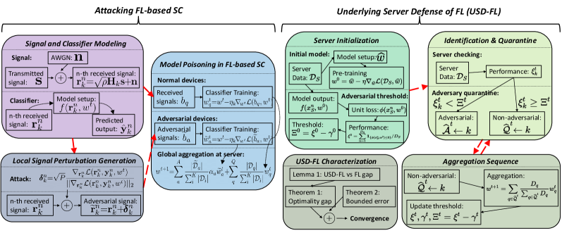
Figure 1: Overall flow of our adversarial framework for FL-based SC and our proposed defense methodology, USD-FL. Both methodologies rely on signal and classifier modeling decisions presented in Sec. III-A.

We develop a novel defense methodology called Underlying Server Defense of Federated Learning (USD-FL) that is able to mitigate the damage caused by adversarial attacks in FL-based SC. Specifically, our proposed defense methodology involves (i) server-side comparisons of device models, (ii) quarantine of devices with likely adversarial perturbations of received signals, and (iii) a modified ML model aggregation rule. Because these individual defense mechanisms involve neither local data nor local model manipulation across network devices, USD-FL can be used in networks with highly independent devices.

I-A Outline and Summary of Contributions:

In the following, we first review relevant literature in both adversarial attacks on and defenses for FL-based SC in Sec. II. Thereafter, our paper is split into two main components: (i) the susceptibility of FL-based SC to model poisoning attacks, and (ii) the proposed defense for FL-based SC against model poisoning attacks (and evasion attacks in particular). We provide a high-level visualization of our workflow in Fig. 1.

Summary of Contributions:

1. FL-Based SC Poisoning Framework: (Sec. III) We propose a framework for poisoning the training process of FL-based SC by perturbing local datasets using potent, but imperceptible, adversarial evasion attacks.

2. Experimental Validation of FL-Based SC Poisoning: (Sec. IV) We demonstrate the susceptibility of signal classifiers to model poisoning through numerical experiments with a real-world AMC dataset in different adversarial environments (e.g., networks of varying size or adversaries). We also reveal that existing server-driven defenses for FL-based SC [9, 10] have difficulty adapting to the wireless setting, due to both AWGN at signal receivers and modulation signal heterogeneity in large-scale wireless networks, thus motivating novel defense methodologies.

3. Defense Methodology for FL-based SC: (Sec. V) We propose USD-FL, a defense methodology based on server verification of device classifiers, and characterize its core control settings.

4. Experimental Validation of USD-FL’s Efficacy: (Sec. VI) We demonstrate that our methodology provides more resilience to adversarial attacks than existing server-driven defenses through experiments with varying types and quantities of adversaries on a real-world AMC dataset.

II Related Work

Adversarial attacks in FL-based SC: Centralized DL-based SC has been shown to be susceptible to adversarial evasion attacks [11, 12, 13, 14]. In these settings, the SC DL classifier is attacked during the inference phase. Specifically, the classifiers are first trained using a collection of labeled radio signals. Then, during test time, the adversary perturbs inputs to induce the trained classifier to output erroneous predictions. Several defenses have been proposed to mitigate such attacks [15, 16], but these methods are designed specifically for test-time attacks in the centralized SC scenario. Our focus, on the other hand, is on adversarial attacks that poison the model training process and lead to a compromised post-training model rather than test-time attacks.

One very effective technique for mitigating evasion attacks on centralized SC systems is adversarial training [17, 18, 19], where the training set is augmented with adversarial examples in order to increase test-time performance in the presence of such attacks. However, adversarial training on samples with high-bounded perturbations results in the model overfitting to adversarial examples, thus reducing classification performance on unperturbed samples [20]. In this work, we utilize this property by augmenting the local training set of particular FL devices with imperceptible adversarial evasion attacks. This, in turn, poisons the global model during training, thus reducing its classification performance.

In terms of FL-based systems, there are two main lines of research. The first line focuses on recovering the training data from FL-related processes. For example, [21, 22, 23] all focus on using classifier gradient information from individual devices to recover original data.

Our goal is in line with the second main line of research, which is the corruption of trained classifier performance [24, 25, 26]. In this context, model poisoning attacks, which aim to corrupt the training process, have been proposed for image processing tasks [24]. Such attacks consist of label flipping [25] and model parameter perturbations [26]. In the former case, the resulting attack potency is low and can be mitigated through global averaging of all model parameters. The latter case relies on perturbing weights after training, which can be detected using existing distributed SC algorithms [27]. Contrary to these works, our proposed attack framework does not rely on perturbing the model parameters after local training, thus bypassing detection mechanisms from previously proposed SC frameworks [1].

Defenses against adversarial devices in FL-based SC: There are two main branches of work in defenses against adversarial attacks in FL. The first branch focuses on preserving data integrity in FL-based systems. For example [28, 29, 30] develop methods that prevent an adversary from recovering user data via reverse engineering classifier gradient information. Our work focuses on the second line of research, which focuses on maintaining the classification performance of FL-based SC.

In terms of preserving classifier performance in FL-style settings, existing works have tended to either rely on device-to-device (D2D) training data comparisons [31, 32] to determine if a device has been compromised by an adversary or focus on server-driven FL defense design [10, 9, 33, 34], which typically consists of modifying aggregations at the server by discarding device models with the largest deviations from the global mean. However, both lines of research have difficulty adapting to the device and training data heterogeneity in wireless networks. In particular, [31] only performs well when network devices have more homogeneous training data distributions, while [32] requires the server to have some clear knowledge of the data distributions across wireless network devices, which a central server in FL-based SC may have difficulty obtaining.

Similarly, research on server-driven defenses for FL also suffers from heterogeneity concerns induced by wireless networks [35, 36]. For example, [9] and [10] both discard model parameters that deviate too far from the mean, while [34] entirely removes a fixed quantity of model parameters farthest from the mean. When network devices have homogeneous local training data and thus more homogeneous model parameters, these server-driven defenses can compare model parameters among network devices to determine if a device has been compromised by an adversary. However, wireless networks contain devices that exhibit heterogeneity with respect to (i) local quality of wireless equipment [37, 38, 39, 40] and (ii) received types of modulated signals [41, 42, 43], both of which naturally lead to heterogeneous local training data and therefore local model parameters with naturally high variance. As a result, these existing defenses can classify the model parameters trained by wireless devices with non-adversarial but noisy signal data (i.e., signals perturbed by non-adversarial AWGN) confused with model parameters poisoned by a genuine adversarial attack. This is especially problematic in FL-based SC as filtering model parameters trained by devices with honest but noisy training data can lead to global aggregations that are further biased towards the model parameters at adversarial devices. We aim to address this problem by providing a defense to effectively detect adversarial devices with low false positive rates for FL-based SC.

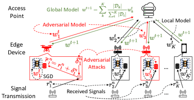
Figure 2: Our proposed FL-based SC framework in which select edge devices train their local models on datasets perturbed with adversarial evasion attacks. As a result, the global model jointly performs aggregation on poisoned and unpoisoned model parameters and subsequently distributes the now-poisoned ML model.

III Attacking FL-based SC - Methodology

In this section, we begin by discussing the preliminary notations and system variables in Sec. III-A. Next, we describe the data perturbation process in Sec. III-B and, finally, we give the overall FL-based model poisoning framework for SC in Sec. III-C. Our proposed framework described throughout this section is shown in Fig. 2.

III-A Signal and Classifier Modeling

We consider an FL framework consisting of $k=1,2,\ldots,K$ participating training devices, where each device contains a local dataset denoted by $\mathcal{D}_{k}$ consisting of $|\mathcal{D}_{k}|$ samples. At each device, $\mathcal{D}_{k}$ is comprised of a set of received signals, which were each transmitted to device $k$ through the channel $\mathbf{h}_{k}=[h_{k}[0],\ldots,h_{k}[\ell-1]]^{T}$, where $\ell$ is the length of the received signal’s observation window. We assume that the channel distribution between the transmitter and each device is independent and identically distributed (i.i.d.). Formally, the $n^{\text{th}}$ signal received at device $k$ is modeled by

$$\mathbf{r}^{n}_{k}=\sqrt{\rho}\mathbf{H}_{k}\mathbf{s}^{n}_{k}+\mathbf{n},$$ (1)

where $\mathbf{s}^{n}_{k}=[s[0],\ldots,s[\ell-1]]$ is the transmitted signal, $\mathbf{H}_{k}=\text{diag}\{h_{k}[0],\ldots,h_{k}[\ell-1]\}\in\mathbb{C}^{\ell\times\ell}$, $\mathbf{n}\in\mathbb{C}^{\ell}$ is complex additive white Gaussian noise (AWGN), and $\rho$ denotes the signal to noise ratio (SNR), which is known at the receiver of each device. Each realization of $\mathbf{r}^{n}_{k}$ of various constellations, and the FL objective is to learn a global signal classifier by training all local models to classify the signal as one of $C$ possible signal constellations.

Although all received signals are complex, $\mathbf{r}^{n}_{k}\in\mathbb{C}^{\ell}$, we denote each signal in terms of its real and imaginary components, $\mathbf{r}^{n}_{k}\in\mathbb{R}^{\ell\times 2}$, where the two columns represent the real and imaginary components of $\mathbf{r}^{n}_{k}$, in order to (i) utilize all signal features during training and (ii) use real-valued DL architectures as overwhelmingly used in DL and FL-based SC.

At the beginning of each training round, $t$, the global model transmits its parameters, $w^{t}$, to each FL device. Each device then trains, using $w^{t}$ as the starting point, its own local model, denoted by $f(\cdot,w^{t}):\mathbb{R}^{\ell\times 2}\rightarrow\mathbb{R}^{C}$, where $f()$ denotes the deep learning classifier (identical architecture at each device) and $(\cdot)$ represents the input. At the termination of the training round, each local device returns $w^{t}_{k}$, which is the model parameters of device $k$ after the completion of training round $t$ on $\mathcal{D}_{k}$, to the global server for aggregation (further discussed in Sec. III-C). After aggregation, the global server transmits the updated model parameters, $w^{t+1}$, for the next round of training. The model prediction, after training round $t$, is given by $\hat{\mathbf{y}}^{n}_{k}=f(\mathbf{r}^{n}_{k},w^{t})$, where $\hat{\mathbf{y}}^{n}_{k}\in\mathbb{R}^{C}$ denotes the predicted output vector of $\mathbf{r}^{n}_{k}$ from $f()$. Moreover, the predicted signal constellation is given by $\text{argmax}_{j}\hskip 2.84526pt\hat{\mathbf{y}}^{n}_{k,j}$, where $\hat{\mathbf{y}}^{n}_{k,j}\in\mathbb{R}$ is the $j^{\text{th}}$ element of $\hat{\mathbf{y}}^{n}_{k}$.

III-B Local Data Perturbation Generation

Here, we describe the process followed by each adversarial device (we show the effects of varying the number of adversarial devices that follow this procedure in Sec. IV-B). Within our proposed framework, a subset of devices, termed adversarial devices, will train on perturbed inputs, beginning at training iteration $t_{0}$, and the remaining devices will continue training on their original unperturbed local datasets. At the beginning of each training iteration, after the local model has received an updated global model, adversarial devices will craft adversarial evasion perturbations on each instance of $\mathbf{r}^{n}_{k}$. The $n^{\text{th}}$ resulting sample is denoted by

$$\widetilde{\mathbf{r}}^{n}_{k}=\mathbf{r}^{n}_{k}+\boldsymbol{\delta}^{n}_{k},$$ (2)

where $\boldsymbol{\delta}^{n}_{k}$ is the adversarial perturbation crafted for the $n^{\text{th}}$ signal on device $k$.

The adversarial perturbation, $\boldsymbol{\delta}^{n}_{k}$, could be crafted at each local device by utilizing common perturbation models such as AWGN or changing the local data completely by e.g., using zero-vectors as training samples or training on signals received from an out-of-distribution channel. However, the injection of AWGN results in less potent attacks to the global model in comparison to our proposed perturbation methodology (as we will show in Sec. IV-B). On the other hand, although changing the local training data may result in more potent attacks, the global model can simply query training samples from each local device to identify the adversarial device. Using adversarial evasion attacks, as we propose, induces a higher attack potency while simultaneously being imperceptible and, thus, is able to withstand FL adversarial attack detectors that rely on querying local data to identify adversarial devices.

To craft an effective and imperceptible perturbation, adversaries will aim to satisfy

$$\underset{\boldsymbol{\delta}}{\text{min}}\quad ||\boldsymbol{\delta}^{n}_{k}||_{2}$$ (3a)

s. t. $$\hskip 1.42262ptf(\mathbf{r}^{n}_{k},w^{t})\neq f(\mathbf{r}^{n}_{k}+\boldsymbol{\delta}^{n}_{k},w^{t}),$$ (3b)

$$||\boldsymbol{\delta}^{n}_{k}||_{2}^{2}\leq P,$$ (3c)

$$\mathbf{r}^{n}_{k}+\boldsymbol{\delta}^{n}_{k}\in\mathbb{R}^{\ell\times 2},$$ (3d)

where $||\cdot||_{2}$ denotes the $l_{2}$ norm and $P$ is the power budget for each adversarial signal. (3a) minimizes power in order to keep the perturbation imperceptible, (3b) changes the prediction of the perturbed sample for a given model, (3c) sets a maximum power, and (3d) keeps $\widetilde{\mathbf{r}}^{n}_{k}$ in the same dimensional space as $\mathbf{r}^{n}_{k}$.

Algorithm 1 FL model poisoning in SC at training iteration $t>t_{0}$, where the adversarial devices train on perturbed inputs.

1:  input: $w^{t}$: global parameter values at training round $t$

2:  for $q=1,\ldots,Q$ do

3:     $\mathcal{B}_{q}\leftarrow$ split $\mathcal{D}_{q}$ into batches

4:     $w^{t}_{q}\leftarrow w^{t}$

5:     for batch $b_{q}\in\mathcal{B}_{q}$ do

6:        $w^{t}_{q}\leftarrow w^{t}_{q}-\eta\nabla_{w^{t}_{q}}\mathcal{L}(b_{q},w^{t}_{q})$

7:     end for

8:  end for

9:  for $a=1,\ldots,A$ do

10:     $\widetilde{\mathcal{D}}_{a}\leftarrow\{\}$

11:     for $\mathbf{r}^{n}_{a}\in\mathcal{D}_{a}$ do

12:        $\boldsymbol{\delta}^{n}_{a}=\sqrt{P}\frac{\nabla_{\mathbf{r}_{\text{k}}^{n}}\mathcal{L}(\mathbf{r}^{n}_{k},\mathbf{y}^{n}_{k},w^{t})}{||\nabla_{\mathbf{r}_{\text{k}}^{n}}\mathcal{L}(\mathbf{r}^{n}_{k},\mathbf{y}^{n}_{k},w^{t})||_{2}}$

13:        $\widetilde{\mathbf{r}}^{n}_{a}=\mathbf{r}^{n}_{a}+\boldsymbol{\delta}^{n}_{a}$

14:        add $\widetilde{\mathbf{r}}^{n}_{a}$ to $\widetilde{\mathcal{D}}_{a}$

15:     end for

16:     $\widetilde{\mathcal{B}}_{a}\leftarrow$ split $\widetilde{\mathcal{D}}_{a}$ into batches

17:     $\widetilde{w}^{t}_{a}\leftarrow w^{t}$

18:     for batch $\widetilde{b}_{a}\in\widetilde{\mathcal{B}}_{a}$ do

19:        $\widetilde{w}^{t}_{a}\leftarrow\widetilde{w}^{t}_{a}-\eta\nabla_{\widetilde{w}^{t}_{a}}\mathcal{L}(\widetilde{b}_{a},\widetilde{w}^{t}_{a})$

20:     end for

21:  end for

22:  $w^{t+1}=\sum_{a}^{A}\frac{|\widetilde{\mathcal{D}}_{a}|}{\sum_{i}^{K}|\mathcal{D}_{i}|}\alpha_{a}\widetilde{w}^{t}_{a}+\sum_{q}^{Q}\frac{|\mathcal{D}_{q}|}{\sum_{i}^{K}|\mathcal{D}_{i}|}w^{t}_{q}$

23:  return  $w^{t+1}$

Due to its excessive nonlinearity, however, (3) is difficult to solve using traditional optimization methods. Thus, we approximate its solution using the fast gradient sign method (FGSM) [44]. The FGSM perturbation for our proposed FL-based SC model is given by

$$\boldsymbol{\delta}^{n}_{k}=\sqrt{P}\frac{\nabla_{\mathbf{r}^{n}_{\text{k}}}\mathcal{L}(\mathbf{r}^{n}_{k},\mathbf{y}^{n}_{k},w^{t})}{||\nabla_{\mathbf{r}^{n}_{\text{k}}}\mathcal{L}(\mathbf{r}^{n}_{k},\mathbf{y}^{n}_{k},w^{t})||_{2}},$$ (4)

where

$$\mathcal{L}(\mathbf{r}^{n}_{k},\mathbf{y}^{n}_{k},w^{t})=\sum_{j=1}^{C}\mathbf{y}^{n}_{k,j}\text{log}(\hat{\mathbf{y}}^{n}_{k})$$ (5)

is the cross entropy loss with $\mathbf{y}^{n}_{k,j}$ denoting the $j^{\text{th}}$ element of the true label vector corresponding to $n^{\text{th}}$ sample on the $k^{\text{th}}$ device and $\nabla_{\mathbf{r}_{\text{k}}}\mathcal{L}(\mathbf{r}^{n}_{k},\mathbf{y}^{n}_{k},w^{t})$ denotes the gradient of $\mathcal{L}(\mathbf{r}^{n}_{k},\mathbf{y}^{n}_{k},w^{t})$ w.r.t. $\mathbf{r}^{n}_{k}$. Finally, $\sqrt{P}/||\nabla_{\mathbf{r}_{\text{k}}}\mathcal{L}(\mathbf{r}^{n}_{k},\mathbf{y}^{n}_{k},w^{t})||_{2}$ is the scaling factor used to satisfy the power constraint in (3c).

The objective of each adversarial device is to overfit their local model to the perturbed dataset generated using (2) and (4) for each training sample. We will denote the batch of $N$ perturbed samples at an adversarial device $a$ as $\widetilde{b}_{a}=\{(\widetilde{\mathbf{r}}^{n}_{a},\mathbf{y}^{n}_{a})\}_{n=1}^{N}$ and the weights at the end of training round, $t$ as $\widetilde{w}^{t}_{a}$. Similarly, the batch of $N$ unperturbed inputs as well as the weights at the end of training round $t$ at a non-adversarial device $q$ will be denoted as $b_{q}=\{(\mathbf{r}^{n}_{q},\mathbf{y}^{n}_{k})\}_{n=1}^{N}$ and $w^{t}_{q}$, respectively. For the each devices’ complete dataset (i.e., the superset of all possible local batches), we use $\widetilde{\mathcal{D}}_{a}$ and $\mathcal{D}_{q}$ for adversarial device $a$ and non-adversarial device $q$ respectively.

III-C Model Poisoning in FL-Based Signal Classification

To begin each training round, $t$, in the FL AMC training process, the global model will transmit $w^{t}$ to each participating FL device. Note that when $t=0$ (i.e., the first round of training), $w^{0}$ is initialized at the server, and subsequently synchronized across the network. After receiving $w^{t}$, each FL device $k$ will train $f(\cdot,w^{t})$ on $\mathcal{D}_{k}$. The model parameters of the $a^{\text{th}}$ adversarial device will be updated, beginning on training round $t_{0}$, according to

$$\widetilde{w}^{t}_{a}=w^{t}-\eta\hskip 2.84526pt\nabla_{w^{t}}\mathcal{L}(\widetilde{b}_{a},{w}^{t}),$$ (6)

while the model parameters of the $q^{\text{th}}$ non-adversarial device, along with adversarial devices prior to training round $t_{0}$, will be updated according to

$$w^{t}_{q}=w^{t}-\eta\hskip 2.84526pt\nabla_{w^{t}}\mathcal{L}(b_{q},w^{t}),$$ (7)

where $\eta$ is the learning rate. At the termination of training round $t$, each FL device will transmit its updated model parameters back to the global server. Although non-adversarial devices will transmit $w^{t}_{q}$ to the global model, adversarial devices will transmit $\alpha_{a}\hskip 1.42262pt\widetilde{w}^{t}_{a}$, where $\alpha_{a}>0$ is a scaling factor used at adversarial device $a$ that can be used to make the effect of the perturbed weights more potent at the global model. Note that $\alpha_{a}=1$ corresponds to not scaling the trained weights. In addition, each FL device will also transmit $|\mathcal{D}_{k}|$ to the global model for appropriate parameter scaling from each participating device during global aggregation.

The global model will then perform a global aggregation using the received weights. From the perspective of the server, the aggregation scheme used to generate the model parameters for the next device training iteration has form:

$$w^{t+1}=\sum_{k}^{K}\frac{|\mathcal{D}_{k}|}{\sum_{i}^{K}|\mathcal{D}_{i}|}w^{t}_{k},$$ (8)

where $K$ is the total number of FL devices. However, the true aggregation process, taking the effect of the adversarial devices into account, is given by

$$w^{t+1}=\sum_{a}^{A}\frac{|\widetilde{\mathcal{D}}_{a}|}{\sum_{i}^{K}|\mathcal{D}_{i}|}\alpha_{a}\widetilde{w}^{t}_{a}+\sum_{q}^{Q}\frac{|\mathcal{D}_{q}|}{\sum_{i}^{K}|\mathcal{D}_{i}|}w^{t}_{q},$$ (9)

where $A$ and $Q$ are the total number of adversarial and non-adversarial devices, respectively, and $K=A+Q$. As a result of this design, the global model will suffer in convergence performance despite not aggregating the local data to a centralized location. The complete overview of our model poisoning framework is given in Algorithm 1.

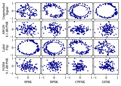
Figure 3: Waveform constellation visualizations for four RML labels: 8PSK, BPSK, CPFSK, and GFSK. The top row depicts received signals with no additive perturbations added at the local device. The AWGN and FGSM perturbations are both shown with $\text{PNR}=8.1$ dB and visually appear similar. The label flipping attack, shown in the third row, changes the true underlying label, for example the BPSK and CPFSK constellations are flipped.

IV Evaluation of Attack Framework

Here, we begin in Sec. IV-A by discussing the DL classification architecture employed at each local model as well as the dataset used in our evaluation. Then, in Sec. IV-B, we present the results of our numerical simulations in which we consider a variety of different adversarial operating environments.

IV-A FL Classification Architecture and Dataset

Each device trains a local DL classifier with the VT-CNN2 architecture [2]. Specifically, each local classifier is composed of 2 sequential convolutional layers with 256 and 80 feature maps, consisting of $1\times 3$ and $2\times 3$ kernel sizes, respectively, followed by a 256 unit dense layer and a $C$ dimensional output layer. Each intermediate layer applies the ReLU activation, and the output layer applies the softmax activation. Thus $\hat{\mathbf{y}}^{n}_{k,j}$ can be interpreted as the probability of the $n^{\text{th}}$ input from the $k^{\text{th}}$ device belonging to the $j^{\text{th}}$ class. We use $\eta_{k}=0.001\hskip 2.84526pt\forall\hskip 2.84526ptk$, and we set $\alpha_{a}=1\hskip 2.84526pt\forall\hskip 2.84526pta$ to isolate the effect of evasion attacks.

To evaluate our poisioning framework, we employ the RadioML2016.10a dataset (RML), which is an automatic modulation classification (AMC) dataset commonly used to benchmark the effectiveness of wireless communications algorithms for radio signal classification. The dataset consists of signals in the following ten modulation constellations stored at an SNR of 10 dB: 8PSK, AM-DSB, BPSK, CPFSK, GFSK, PAM4, QAM16, QAM64, QPSK, and WBFM. In total, we apply a $75\%/25\%$ train/test split, resulting in $45$K training samples, split among the participating clients, and $15$K testing samples contained at the global server.

Each RML signal is normalized to unit energy and has observation window of length $\ell=128$. We depict the RML constellations in the uppermost row of Fig. 3, and show the signals after perturbing using FGSM as well as after perturbing using AWGN (baseline) and label flipping (baseline) in Fig. 3.

We measure the potency of the local perturbations in terms of the perturbation to noise ratio (PNR) given by

$$\text{PNR [dB]}=\text{PSR [dB]}+\text{SNR [dB]},$$ (10)

where PSR is the perturbation to signal ratio.

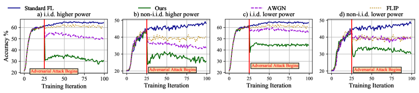
Figure 4: Training performance of high and low power perturbations for a network with $30\%$ adversarial devices. High power perturbations at $8.1$ dB PNR are shown in a) and b) and low power perturbations at $6.7$ dB PNR are shown in c) and d). Lower accuracy indicates higher adversarial impact. For both i.i.d. and non-i.i.d. scenarios, our algorithm yields the most potent model poisoning attack.

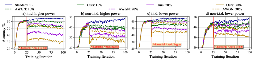
Figure 5: Varying the proportion of network compromised by adversaries from $10\%$ to $30\%$. High power perturbation ($8.1$ dB PNR) experiments are in a) and b) and low power perturbations ($6.7$ dB PNR) experiments are in c) and d). Our algorithm remains the most potent even as the quantity of adversarial devices varies, indicated within the legend.

IV-B Performance Evaluation

We first demonstrate the effectiveness of our method, relative to the baselines, in Sec IV-B1. We then show that evasion-based attacks directly scale with the number of adversaries in the network in Sec IV-B2.

Unless otherwise stated, in our evaluations, we consider a network of $K=10$ devices consisting of classifiers based on the VT-CNN2 architecture described in Sec. IV-A in both i.i.d. and non-i.i.d. signal distributions among devices. In an i.i.d. environment, our network devices all contain the same quantity of local data and have local data sampled uniformly at random from each class of the full training dataset. In the non-i.i.d. case, devices have data quantity chosen randomly from $\mathcal{N}(4500,45)$ and data randomly sampled from only three labels as in [45]. After training iteration $t_{0}=25$, $30\%$ of the network is compromised by adversarial influence, and begins training on perturbed local datasets.

IV-B1 Baseline Comparison

We compare our framework to two baseline methods: data poisoning via AWGN and label flipping (FLIP). AWGN attacks inject random Gaussian noise into the training data at the local devices while label flipping intentionally mislabels local training data. We choose to compare against these baselines since, similar to our method, they both rely on intentional manipulations of local training data to poison model aggregations and thus the global model.

In our evaluation, we vary the power of the perturbation to assess its effect on the potency of the attack. For the high power scenario in Fig. 4a) and 4b), we set the PNR of both our method as well as the AWGN baseline to $8.1$ dB. Our methodology yields the most potent training performance for both i.i.d. and non-i.i.d. scenarios. In the i.i.d. case in Fig. 4a), our algorithm reduces classification performance, at the termination of training, by over $31\%$, which is a roughly $20\%$ increase over AWGN and a $30\%$ increase over FLIP. Similarly, in the non-i.i.d. case in Fig. 4b), our method reduces the accuracy by over $22\%$, which is $8\%$ more than AWGN and $14\%$ more than FLIP.

In the low power scenario in Fig. 4c) and 4d), the AWGN attack and our algorithm both have $6.7$ dB PNR. FLIP is PNR independent and, thus, has the same results from Fig. 4a) and 4b). Here, our methodology continues to outperform all baselines. In the i.i.d. case, we reduce the classification performance, at the termination of training, by over $19\%$, which corresponds to a $11\%$ improvement over AWGN and a $14\%$ improvement over FLIP. Furthermore, in the non-i.i.d. scenario, our algorithm reduces performance by $18\%$, outperforming, potency-wise, both AWGN and FLIP by $9\%$.

The reduction in nominal impact of all evasion attacks in non-i.i.d. environments seen throughout Fig. 4 is the result of an innate property of FL. Specifically, in non-i.i.d. scenarios, devices and thus adversaries may not have data from all possible labels. As a result, the adversaries can only bias the ML model’s classification performance on the specific labels that they have corresponding data for. Consequently, after model aggregations, the global ML model display weaker classification on underlying labels present at the adversaries.

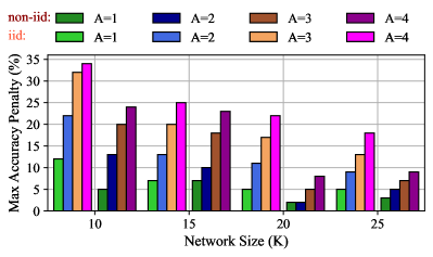
Figure 6: The impact of network size on reducing the classification performance. Light and dark colors indicate i.i.d. and non-i.i.d. underlying data distributions respectively. Larger networks require more nominal adversaries to achieve significant accuracy penalties.

IV-B2 Network Scaling Effects

Next, we evaluate the potency of our framework in Fig. 5, where we vary the proportion of the network compromised by adversarial devices from $10\%$ to $30\%$. Label flipping attacks do not necessarily become more potent as more adversaries enter the network, as a simple label flipping attack always attacks/flips the same labels and, as a result, the total number of compromised labels can be independent of the number of adversaries. Therefore, to clearly demonstrate the impact of more compromised devices, we omit the FLIP attack. Otherwise, the experimental setup for Fig. 5 remains the same as that for Fig. 4.

In the high power scenario in Fig. 5a) and 5b), our method reduces final classification performance by $11\%$ to over $31\%$ as the proportion of adversarial devices increases from $10\%$ to $30\%$ for the i.i.d. case, and by $8\%$ to over $22\%$ as the proportion of adversarial devices increases from $10\%$ to $30\%$ for the non-i.i.d. case. In the low power case of Fig. 5c) and 5d), our algorithm reduces final accuracy by $8\%$ to over $19\%$ as the proportion of adversarial devices increases from $10\%$ to $30\%$ for the i.i.d. scenario, and by $7\%$ to $18\%$ as the proportion of adversarial devices increases from $10\%$ to $30\%$ for the non-i.i.d. scenario. In these cases, when the proportion of adversaries increases 3x, the degradation increases by almost 3x. The classification degradation grows almost linearly with the proportion of adversaries. Regardless of the total number of network adversaries, our methodology continues to either outperform or match their baseline counterparts while remaining imperceptible to the global model.

We also investigate the impact of incrementing the quantity of adversarial devices, $A$, in networks of varying size in Fig. 6. In Fig. 6, to better capture the effect of adversaries in varying network sizes, we show the max accuracy penalty relative to the unperturbed scenario for four different network sizes. Increasing network size with a constant number of adversaries decreases the proportion of devices that are adversarial. Thus, to get the same level of adversarial influence in larger networks, we would nominally require more adversaries. Our results in Fig. 6 confirm this intuition for both the i.i.d. and non-i.i.d. cases, and solidifies the insights from Fig. 5. For example, $4$ adversaries in the i.i.d. case yields over $30\%$ accuracy penalty in a network of $10$ devices but only $17\%$ accuracy penalty in a network of $25$ devices. A similar trend holds for the non-i.i.d. case with $4$ adversaries yielding roughly $24\%$ accuracy penalty in a network of $10$ devices but only $8\%$ in a network of $25$ devices. The nominal decrease in accuracy penalty in non-i.i.d. settings as compared to i.i.d. settings shown in Fig. 6 further confirms that non-i.i.d. scenarios are also more resilient to adversarial evasion attacks. The reasons for this are the same as those presented in Sec IV-B1. Essentially, in the non-i.i.d. scenario, adversaries only contain data from a select subset of labels and, as a result, are only able to perturb the model’s classification power on those specific labels.

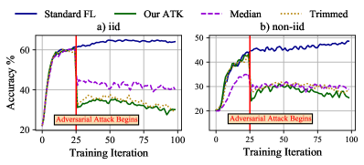
Figure 7: Existing server-driven defenses for FL demonstrate difficulty defending FL-based SC against adversarial poisoning attacks. In both i.i.d. and non-i.i.d. settings, existing server-driven defenses have difficulty countering the potency of the proposed adversarial framework.

IV-B3 Server-Driven Defenses

Finally, we evaluate the performance of the proposed adversarial framework against popular server-driven defenses from literature in Fig. 7, which consists of a network with $30\%$ adversarial devices. In particular, we investigate the ability of the Median and Trimmed-Mean defenses for FL [9, 8] against the proposed adversarial framework with 8.1 dB PNR. For trimmed-mean, we select the largest and smallest coordinates to discard prior to aggregation.

We first investigate the ability of baseline server-driven defenses to mitigate adversarial perturbations in the i.i.d. scenario of Fig. 7a). Here, we show the performance of median and trimmed-mean (trimmed) defenses against the proposed adversarial framework. While the two server-driven defenses are able to offer a marginal improvement over undefended FL-based SC (i.e., the solid green line), the proposed adversarial framework remains able to significantly compromise FL-based SC. Specifically, versus median and trimmed-mean defenses, our framework is still able to decrease classification accuracy, relative to unperturbed standard FL, by roughly $20\%$ and over $30\%$ respectively.

Similarly, in the non-i.i.d. setting of Fig. 7b), existing server-driven defenses for FL experience difficulty in the SC setting. Both defence methodologies are able to demonstrate a marginal improvement of roughly $2\%$ over undefended FL-based SC. However, versus either server-driven defense, our framework remains able to decrease classification accuracy by over $17\%$ relative to unperturbed standard FL.

These effects are because wireless networks and thus the FL-based SC problem contain extensive data heterogeneity, owing to both (i) the presence of varying levels of non-adversarial AWGN and (ii) different types of modulated signals across wireless network devices, that leads to highly heterogeneous model parameters across wireless devices. While these forms of heterogeneity are natural and non-adversarial in wireless networks, they confuse existing FL defenses, leading them to filter non-adversarial model parameters instead of adversarial ones.

V Underlying Server Defense of FL

As existing server-driven methods to defend standard FL against adversarial attacks have difficulty adapting to FL-based SC, there is a need for novel defense methodologies for the SC problem, especially when wireless devices have non-i.i.d. local signal data. To this end, we propose a novel defense methodology, USD-FL, in Fig. 8 to overcome these underlying hurdles in FL-based SC.

At a high level, our proposed USD-FL methodology leverages the ability of the central server to perform light pre-training, commonly done in FL research [46, 47, 48, 49]. Thereafter, the server can evaluate the quality of network devices’ trained model parameters by checking their SC accuracy on the pre-training dataset, and determine whether an adversarial attack has occurred. In the following, we describe our methodology in four components: (i) server design in Sec. V-A, (ii) identification and quarantine of adversarial devices in Sec. V-B, (iii) modification of global aggregations in Sec. V-C, and (iv) characterization of optimality gap in Sec. V-D.

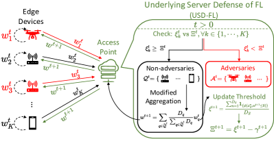
Figure 8: Simplified view of our proposed USD-FL methodology in which the server plays an active role in filtering adversarial vs non-adversarial devices. After determining the set of non-adversarial devices, the server performs a modified aggregation, and uses the new model parameters to update a performance threshold for future adversary determinations.

V-A Server Design and Initialization

As in Fig. 2 from Sec. III, the central server $S$ transmits its parameters $w^{t}$ to all edge devices following each and every aggregation. We assume the central server $S$ contains an unperturbed dataset $\mathcal{D}_{S}$ collected from historically received, non-adversarial signals, with a total of $D_{S}$ unique data samples drawn similarly as those in Sec. III.

Prior to starting the FL process, the server $S$ will pre-train $f(\cdot,w^{i})$ on $\mathcal{D}_{S}$, where ${w}^{i}$ is a set of randomly initialized model parameters. For $t>0$, the global parameters $w^{t}$ will have the form specified in Sec. V-C, and the server will measure the SC accuracy of each $w^{t}$ on the original pre-training dataset $\mathcal{D}_{S}$ as follows:

$$\xi^{t}=\frac{\sum_{n=1}^{D_{S}}{\mathds{1}_{\{\phi(x^{n}_{S},w^{t})\leq 0\}}}}{D_{S}},$$ (11)

where $\phi(x^{n}_{S},w^{t})=|\operatorname*{argmax}_{i}f(x^{n}_{S},w^{t})-\operatorname*{argmax}_{j}\boldsymbol{y}^{n}_{S,j}|$ as $f(x^{n}_{S},w^{t})=\hat{\boldsymbol{y}}^{n}_{S,i}$ (as explained in Sec. III), and

$$\mathds{1}_{\{\phi(x^{n}_{S},w^{t})\leq 0\}}=\begin{cases}1&\text{If }\phi(x^{n}_{S},w^{t})\leq 0\\ 0&\text{Otherwise.}\end{cases}$$ (12)

V-B Identification and Quarantine of Adversaries

All network devices $k\in\mathcal{K}$ will locally train a SC with model parameters $w^{t}_{k}$ based on the epoch $t$ and the update rules specified in Sec. III. Then, each adversarial device $a\in\mathcal{A}$ will transmit scaled model parameters $\alpha_{a}\widetilde{w}^{t}_{a}$ to the server while each non-adversarial device $q\in\mathcal{Q}$ will transmit model parameters $w^{t}_{q}$ instead.

Next, the server $S$ can evaluate the SC performance of devices’ model parameters on the pre-training dataset $\mathcal{D}_{S}$ in order to identify and subsequently quarantine potential adversarial devices. Specifically, for each $k\in\mathcal{K}$, the server $S$ can obtain a device-specific classifier accuracy $\xi^{t}_{k}$ on $D_{S}$ of the following form

$$\xi^{t}_{k}=\frac{\sum_{n=1}^{D_{S}}\mathds{1}_{\{\phi(x^{n}_{S},w^{t}_{k})\leq 0\}}}{D_{S}},$$ (13)

while noting that $w^{t}_{k}=\alpha_{a}\widetilde{w}^{t}_{a}$ when $k$ indexes an adversarial device. Simultaneously, the server $S$ determines an accuracy threshold $\Xi^{t}$ based on the empirical global accuracy $\xi^{t}$ and a margin $\gamma^{t}$ to account for extreme network heterogeneity (which can result in non-adversarial devices exhibiting a temporary and marginal decrease in performance). Formally,

$$\Xi^{t}=\xi^{t}-\gamma^{t},\hskip 4.2679pt\xi^{t}\geq\gamma^{t}>0.$$ (14)

Setting $\gamma^{t}=\xi^{t}$ is equivalent to having no threshold, i.e., a return to standard FL susceptible to adversarial poisoning attacks. The selection process for $\gamma^{t}$ can be adjusted based on the heterogeneity across network devices. For instance, in environments with highly non-i.i.d. data across network devices, $\gamma^{t}$ can be larger to reduce the chance that non-adversarial devices get filtered. We will explain our choice of $\gamma^{t}$ in Sec. VI. Through comparison with $\Xi^{t}$, the server $S$ can determine if a device $k$ exhibits adversarial characteristics ($\xi^{t}_{k}<\Xi^{t}$) or not ($\xi^{t}_{k}\geq\Xi^{t}$). Thereafter, $S$ can partition devices into likely adversarial devices $\widehat{\mathcal{A}}^{t}$ and non-adversarial devices $\widehat{\mathcal{Q}}^{t}$, analogously to the sets of true adversarial devices $\mathcal{A}$ and non-adversarial devices $\mathcal{Q}$.

V-C Modified Aggregation Rule

Post-partition of $\mathcal{K}$, the server $S$ can modify the global aggregation rule, obtaining

$$w^{t+1}=\sum_{q\in\widehat{\mathcal{Q}}^{t}}\frac{D_{q}}{\sum_{q\in\widehat{\mathcal{Q}}^{t}}D_{q}}w^{t}_{q}\equiv\sum_{k\in\mathcal{K}}\frac{\mathds{1}_{\{\xi^{t}_{k}\geq\Xi^{t}\}}w^{t}_{k}D_{k}}{\sum_{k\in\mathcal{K}}\mathds{1}_{\{\xi^{t}_{k}\geq\Xi^{t}\}}D_{k}},$$ (15)

rather than the compromised aggregation procedure in (9). The expanded form of USD-FL’s global aggregation rule - right hand side of (15) - highlights server control over the aggregation. Specifically, by adjusting $\gamma^{t}$, the server $S$ controls the threshold $\Xi^{t}$, and the set of non-adversarial devices $\widehat{Q}^{t}$ used for aggregation.

Next, $S$ synchronizes model parameters at all devices, including those at devices perceived to be compromised by adversarial poisoning attacks, to the latest global model parameters $w^{t+1}$ from (15). This synchronization is performed in order to minimize the consequences of false-positives in the adversary detection process, as, in highly heterogeneous wireless networks, non-adversarial devices may occasionally fall beneath the server threshold $\Xi^{t}$.

Simultaneously, the server uses the new $w^{t+1}$ to update the empirical accuracy $\xi^{t+1}$ via (11), which in turn updates the accuracy threshold $\Xi^{t+1}$. It is important to continuously update the accuracy threshold $\Xi^{t}$ because adversarial poisoning attacks may have bounded impacts [16, 26, 50] and, therefore, adversarial devices $a\in\mathcal{A}$ may yield $\xi^{t}_{a}\geq\Xi^{0}$ for large $t$. In this manner, our proposed USD-FL methodology, summarized in Algorithm 2, is able to continuously defend against adversarial poisoning attacks from true adversaries $a\in\mathcal{A}$.

Algorithm 2 Underlying Server Defense of Federated Learning (USD-FL).

1:  input: $\mathcal{D}_{S}$: unperturbed dataset at the server $S$

2:  input: ${w}^{i}$: randomly initialized global model parameters

3:  input: $\eta$: learning rate of model training

4:  $t=0$

5:  $w^{0}\leftarrow{w}^{i}-\eta_{S}\nabla_{{w}^{i}}\mathcal{L}(\mathcal{D}_{S},{w}^{i})$

6:  while True do

7:     $\xi^{t}=\sum_{n=1}^{D_{S}}{\mathds{1}_{\{\phi(x^{n}_{S},w^{t})\leq 0\}}}/{D_{S}}$

8:     $\Xi^{t}=\xi^{t}-\gamma^{t}$

9:     for $k=1,\ldots,K$ do

10:        $w^{t}_{k}\leftarrow w^{t}$

11:        device $k$ locally updates $w^{t}_{k}$

12:        $w^{t}_{k}$ sent to server $S$

13:     end for

14:     $\widehat{\mathcal{A}}^{t}\leftarrow\{\}$, $\widehat{\mathcal{Q}}^{t}\leftarrow\{\}$

15:     for $k=1,\ldots,K$ do

16:        $\xi^{t}_{k}\leftarrow\sum_{n=1}^{D_{S}}\mathds{1}_{\{\phi(x^{n}_{S},w^{t}_{k})\leq 0\}}/{D_{S}}$

17:        if $\xi^{t}_{k}<\Xi^{t}$ then

18:           add $k$ to $\widehat{\mathcal{A}}^{t}$

19:        else

20:           add $k$ to $\widehat{\mathcal{Q}}^{t}$

21:        end if

22:     end for

23:     $w^{t+1}=\sum_{q\in\widehat{\mathcal{Q}}^{t}}\frac{D_{q}}{\sum_{q\in\widehat{\mathcal{Q}}^{t}}D_{q}}w^{t}_{q}$

24:     $t=t+1$

25:  end while

V-D Optimality gap of USD-FL

Because the aggregation rule of USD-FL involves filtering adversarial devices entirely, (15) is effectively training a global model on a sampled subset of training data. This data sampling effect means that USD-FL will have a performance gap relative to standard FL without any adversaries. Since standard FL has been proven theoretically to converge [51, 52, 53] to an optimal set of model parameters $w^{*}$, we can show that, if USD-FL converges to unperturbed standard FL, then USD-FL should by extension also converge to an optimal point.

To this end, we first define a common set of assumptions used in literature [51, 54] for general loss functions $\mathcal{L}$:

Assumption 1.

We assume that $\mathcal{L}(w)$ is $\rho$-Lipschitz, i.e., $\|\mathcal{L}(w)-\mathcal{L}(w^{\prime})\|\leq\rho\|w-w^{\prime}\|$ $\forall w,w^{\prime}$, and $\mu$-strongly convex, i.e., $\mathcal{L}(w^{\prime})\geq\mathcal{L}(w)+(w^{\prime}-w)^{T}\nabla\mathcal{L}(w)+\frac{\mu}{2}\|w-w^{\prime}\|^{2}$ $\forall w,w^{\prime}$.

In Assumption 1, we use $\mathcal{L}(w)$ to refer to the classification loss of $w$ on the data across all network devices, i.e., $\mathcal{L}(w)=\mathcal{L}(\mathcal{D}_{K},w)$ where $\mathcal{D}_{K}\triangleq\cup_{k\in\mathcal{K}}\mathcal{D}_{k}$. When we refer to $\mathcal{L}(w)$ on a particular device $k$’s dataset $\mathcal{D}_{k}$, we will denote it by $\mathcal{L}(\mathcal{D}_{k},w)$. In addition, $\mathcal{L}(w)$ retains the properties first described in Sec. III.

Lemma 1 (Gap between USD-FL and standard FL).

Given a set of standard FL parameters $\widehat{w}^{t}$, the gap between standard FL and USD-FL is bounded $\forall t$ by:

$$\mathcal{L}(\widehat{w}^{t})-\mathcal{L}(w^{t})\leq\zeta(\Xi^{t})^{T}\nabla\mathcal{L}(w^{t})+\frac{\rho}{2}\left\|\zeta(\Xi^{t})\right\|^{2},$$ (16)

where

$$\zeta(\Xi^{t})\triangleq\bigg{(}\sum_{k^{{}^{\prime}}\in\mathcal{K}}\mathds{1}_{\{\xi^{t}_{k^{{}^{\prime}}}\geq\Xi^{t}\}}D_{k^{{}^{\prime}}}\sum_{k\in\mathcal{K}}w_{k}D_{k}$$ (17)

$$-\sum_{k\in\mathcal{K}}D_{k}\sum_{k^{{}^{\prime}}\in\mathcal{K}}\mathds{1}_{\{\xi^{t}_{k^{{}^{\prime}}}\geq\Xi^{t}\}}w_{k^{{}^{\prime}}}D_{k^{{}^{\prime}}}\bigg{)}$$

$$\bigg{(}\sum_{k^{{}^{\prime}}\in\mathcal{K}}\mathds{1}_{\{\xi^{t}_{k^{{}^{\prime}}}<\Xi^{t}\}}D_{k^{{}^{\prime}}}\sum_{k\in\mathcal{K}}D_{k}\bigg{)}^{-1}.$$

Proof.

Combining the $\rho$-Lipschitz and $\mu$-strongly convex properties of $\mathcal{L}$ and noting that $\widehat{w}^{t}-w^{t}=\zeta(\Xi^{t})$ by definition yields the result. ∎

If USD-FL does not set a threshold (i.e., $\Xi^{t}=0$), then all devices will exhibit $\xi^{t}_{k}\geq\Xi^{t}$. Correspondingly, $\zeta(\Xi^{t})\rightarrow 0$ and Lemma 1 converges to 0, confirming intuition that USD-FL and standard FL will yield the same result when the set of perceived adversaries is empty (i.e., $\widehat{\mathcal{A}}^{t}=\emptyset$). Conversely, if USD-FL sets a galactic threshold (i.e., $\Xi^{t}\rightarrow\infty$), then no device will exhibit $\xi^{t}_{k}\geq\Xi^{t}$ and the right hand side of (16) grows large.

Lemma 1 highlights how the gap between USD-FL and standard FL is tightly controlled by $\Xi^{t}$, the adversary detection threshold. USD-FL favors high performing devices with large $\Xi^{t}$, which, on the flip side, can increase the gap to standard FL. We next define a theoretical term in the path to derive the optimality gap of the USD-FL algorithm.

Definition 1 (Gradient loss differential between USD-FL and standard FL).

USD-FL only computes weighted gradients from a subset of the total network datasets. Thus, there is an instantaneous differential between USD-FL and FL gradients, which we define below $\forall t$:

$$e^{t}(w^{t})=\frac{K-\widehat{Q}^{t}}{K\widehat{Q}^{t}}\sum_{q\in\widehat{\mathcal{Q}}^{t}}\nabla\mathcal{L}(\mathcal{D}_{q},w^{t})-\frac{1}{K}\sum_{a\in\widehat{\mathcal{A}}^{t}}\nabla\mathcal{L}(\mathcal{D}_{a},w^{t}).$$ (18)

We now have all the tools needed to derive the optimality gap of the USD-FL algorithm.

Theorem 1 (Optimality gap of USD-FL).

Assuming training step size $\eta\equiv 1/\rho$, the optimality gap of USD-FL is bounded as follows:

$$\mathcal{L}(w^{t+1})-\mathcal{L}(w^{*})\leq\mathcal{L}(w^{t})-\mathcal{L}(w^{*})$$ (19)

$$+\frac{\mu}{\rho}\bigg{[}\zeta(\Xi^{t})^{T}\nabla\mathcal{L}(w^{t})+\frac{\rho}{2}\left\|\zeta(\Xi^{t})\right\|^{2}\bigg{]}$$

$$+\frac{\mu}{\rho}\left(1-\frac{\mu}{\rho}\right)\bigg{[}\mathcal{L}(w^{*})-\mathcal{L}(\widehat{w}^{t-1})\bigg{]}+\frac{1}{2\rho}\|e^{t}(w^{t})\|^{2}.$$

Proof.

Since $\mathcal{L}$ is $\mu$-strongly convex, we have:

$$\mathcal{L}(w^{t+1})\geq\mathcal{L}(w^{t})+(w^{t+1}-w^{t})^{T}\nabla\mathcal{L}(w^{t})+\frac{\mu}{2}\|w^{t+1}-w^{t}\|^{2}.$$ (20)

Taking the minima of both sides in (20) yields $\mathcal{L}(w^{*})\geq\mathcal{L}(w^{t})-\frac{1}{2\mu}\|\nabla\mathcal{L}(w^{t})\|^{2}$, which after introducing $\mathcal{L}(\widehat{w}^{t})$ to both sides and rearranging yields:

$$2\mu\left(\mathcal{L}(w^{t})-\mathcal{L}(\widehat{w}^{t})+\mathcal{L}(\widehat{w}^{t})-\mathcal{L}(w^{*})\right)\leq\|\nabla\mathcal{L}(w^{t})\|^{2}.$$ (21)

Since $\eta\equiv 1/\rho$, we can combine the expanded update rule of USD-FL, i.e., $w^{t+1}=w^{t}-\eta(\nabla\mathcal{L}(w^{t})+e^{t}(w^{t}))$, with Assumption 1 to start bounding $\mathcal{L}(w^{t+1})-\mathcal{L}({w}^{*})$ as follows:

$$\mathcal{L}({w}^{t+1})-\mathcal{L}({w}^{*})\overset{(a)}{\leq}\mathcal{L}({w}^{t})-\mathcal{L}({w}^{*})$$

$$-\frac{1}{2\rho}\|\nabla\mathcal{L}({w}^{t})\|^{2}+\frac{1}{2\rho}\|e^{t}(w^{t})\|^{2}$$ (22)

$$\overset{(b)}{\leq}\mathcal{L}({w}^{t})-\mathcal{L}({w}^{*})$$

$$-\frac{\mu}{\rho}\left(\mathcal{L}(w^{t})-\mathcal{L}(\widehat{w}^{t})+\mathcal{L}(\widehat{w}^{t})-\mathcal{L}(w^{*})\right)+\frac{1}{2\rho}\|e^{t}(w^{t})\|^{2}$$ (23)

$$\overset{(c)}{\leq}\mathcal{L}({w}^{t})-\mathcal{L}({w}^{*})+\frac{\mu}{\rho}\left(\mathcal{L}(w^{*})-\mathcal{L}(\widehat{w}^{t})\right)$$

$$+\frac{\mu}{\rho}\left(\zeta(\Xi^{t})^{T}\nabla\mathcal{L}(w^{t})+\frac{\rho}{2}\left\|\zeta(\Xi^{t})\right\|^{2}\right)+\frac{1}{2\rho}\|e^{t}(w^{t})\|^{2}$$ (24)

$$\overset{(d)}{\leq}\mathcal{L}({w}^{t})-\mathcal{L}({w}^{*})+\frac{\mu}{\rho}\left(1-\frac{\mu}{\rho}\right)\left(\mathcal{L}(w^{*})-\mathcal{L}(\widehat{w}^{t-1})\right)$$

$$+\frac{\mu}{\rho}\left(\zeta(\Xi^{t})^{T}\nabla\mathcal{L}(w^{t})+\frac{\rho}{2}\left\|\zeta(\Xi^{t})\right\|^{2}\right)+\frac{1}{2\rho}\|e^{t}(w^{t})\|^{2},$$ (25)

where $(a)$ is the result of introducing $\mathcal{L}(w^{*})$ to both sides of $\mathcal{L}(w^{t+1})\leq\mathcal{L}(w^{t})+(w^{t+1}-w^{t})^{T}\nabla\mathcal{L}(w^{t})+\frac{\rho}{2}\|w^{t+1}-w^{t}\|$ (which follows from Assumption 1) and subsequently combining with the expanded update rule of USD-FL, $(b)$ follows from (21), $(c)$ uses the result of Lemma 1, and $(d)$ repeats the previous analysis using standard FL parameters $\widehat{w}$ which have a gradient loss differential of $0$ (as standard FL parameters have no differential relative to themselves - see Definition 1). ∎

Since $\rho$ is the Lipschitz coefficient, we can always find pairs of $\mu$ and $\rho$ such that $\mu/\rho<<1$. The only remaining step to show that USD-FL converges is to prove that $e^{t}(w^{t})$ is bounded which we demonstrate next.

Theorem 2 (Boundedness of $e^{t}(w^{t})$).

Suppose that device data distributions $\mathcal{D}_{k}$ have finite second and third moments. Then there exists constants $\gamma_{q}$ $\forall q\in\widehat{\mathcal{Q}}^{t}$ such that

$$\|e^{t}(w^{t})\|\leq\frac{1}{\widehat{Q}^{t}}\sum_{q\in\widehat{\mathcal{Q}}^{t}}\frac{\gamma_{q}}{\sqrt{D_{q}}}.$$ (26)

Proof.

Rearranging the definition of $e^{t}(w^{t})$ yields:

$$e^{t}(w^{t})=\frac{1}{\widehat{Q}^{t}}\sum_{q\in\widehat{\mathcal{Q}}^{t}}\nabla\mathcal{L}(\mathcal{D}_{q},w^{t})-\frac{1}{K}\sum_{k\in\mathcal{K}}\nabla\mathcal{L}(\mathcal{D}_{k},w^{t}).$$ (27)

Since $\nabla\mathcal{L}(w^{t})=\frac{1}{K}\sum_{k\in\mathcal{K}}\nabla\mathcal{L}(\mathcal{D}_{k},w^{t})$, we can obtain:

$$\|e^{t}(w^{t})\| \overset{(a)}{=}\bigg{\|}\frac{1}{\widehat{Q}^{t}}\sum_{q\in\widehat{\mathcal{Q}}^{t}}\nabla\mathcal{L}(\mathcal{D}_{q},w^{t})-\nabla\mathcal{L}(w^{t})\bigg{\|}$$ (28)

$$\overset{(b)}{\leq}\frac{1}{\widehat{Q}^{t}}\sum_{q\in\widehat{\mathcal{Q}}^{t}}\|\nabla\mathcal{L}(\mathcal{D}_{q},w^{t})-\nabla\mathcal{L}(w^{t})\|$$ (29)

$$\overset{(c)}{\leq}\frac{1}{\widehat{Q}^{t}}\sum_{q\in\widehat{\mathcal{Q}}^{t}}\frac{\gamma_{q}}{\sqrt{D_{q}}},$$ (30)

where $(a)$ is the definition of $\mathcal{L}(w^{t})$, $(b)$ follows from repeated applications of the triangle inequality, and $(c)$ follows from the central limit theorem by viewing $\nabla\mathcal{L}(\mathcal{D}_{q},w^{t})$ as $D_{q}$ samples of $\nabla\mathcal{L}(x_{d},y_{d},w^{t})$ from a distribution with expected value $\nabla\mathcal{L}(w^{t})$. ∎

As a result of Theorem 2, we know that $e^{t}(w^{t})$ is bounded and therefore, via Theorem 1, USD-FL will converge to an optimal set of parameters with a gap as $t\rightarrow\infty$. As filtering adversaries effectively reduces the data that a global model is trained from, a gap between USD-FL in the presence of adversaries versus unperturbed standard FL is expected. We can further verify that there is a gap of USD-FL relative to standard FL when we look at USD-FL convergence in Sec. VI.

VI Evaluation of Defensive Framework

Since the FL and SC architectures remain the same as those for the attack evaluation from Sec. IV, we will omit their description here. We instead describe the hyperparameter setup for USD-FL and baseline defenses in Sec. VI-A, before presenting a thorough evaluation of USD-FL relative to baseline defenses for FL-based SC and to various adversarial attacks against FL-based SC in Sec. VI-B.

VI-A Defense Configurations for FL-based SC

For USD-FL, the server pre-trains an initial global classifier using a static reserve dataset $\mathcal{D}_{S}$ of 5k signals randomly sampled without replacement from the training portion of the RML dataset. Specifically, we used a $75\%/25\%$ train/test split to obtain 45K training samples and 15k testing samples from the RML dataset, identical to the evaluation framework used in Sec. IV. The server then performs a single round of pre-training on its reserve dataset, and subsequently follows the steps outlined in Algorithm 2, with $\gamma^{t}$ controlled so that $\gamma^{t}=0.2\xi^{t}$ for i.i.d. scenarios and $\gamma^{t}=0.4\xi^{t}$ for non-i.i.d. scenarios. The value of $\gamma^{t}$ is larger for non-i.i.d. settings in order to reduce the accuracy threshold $\Xi^{t}$ as non-adversarial devices may exhibit greater data variance and thus be filtered out by a high $\Xi^{t}$ threshold. At the device level, local signal datasets and trained local models are obtained in the same way as that in Sec. IV. The server will then evaluate the quality of devices’ local models on its reserve dataset, producing a set of performance estimates $\xi^{t}_{k}$ for all devices $k\in\mathcal{K}$.

The two baseline server-driven defenses for FL-based SC are median [9, 8] and trimmed-mean [9, 8]. Specifically the median defense selects the median classifier parameter across all network devices, and thus is applied in the same way to all distributed SC networks regardless of quantity of adversaries. On the other hand, the trimmed-mean defense, referred to as “trimmed” for conciseness, first removes the largest and smallest $z$ classifier parameters and subsequently takes the average of the remaining ones. Since the exact quantity of network adversaries is unknown apriori, trimmed must estimate a $z$ value prior to FL-based SC training. In this regard, we set $z=1$ so that trimmed is consistent throughout all of our experiments in the following sections (as well as those in Sec. IV). Importantly, these two baseline defenses are both server-driven defenses similar to USD-FL, so the resulting comparisons are both fair and reveal the nuances of USD-FL.

VI-B Performance Evaluation

In the following experimental results, we investigate four core aspects: (i) the effectiveness of USD-FL versus other defensive baselines, (ii) the false-positive rate of all defense methodologies, (iii) the computation time of the defenses, and (iv) the performance of USD-FL versus various types of evasion attacks. All figures and tables are the average of three independent simulations.

VI-B1 Defense methodology comparison

In Table I, we compare the performance of various defense methodologies against the adversarial attack for FL-based SC from Sec. III with PNR of 8.1 dB. Specifically, we use “Acc” to refer to Accuracy, “M” to refer to the median defense [9, 8], “T” to refer to the trimmed defense [9, 8], and “U” to refer to USD-FL. In the i.i.d. setting, USD-FL consistently yields the highest final classifier accuracies for networks with 10%-40% adversarial devices. Furthermore, when comparing the final accuracy of USD-FL versus that of unperturbed standard FL, we can see that USD-FL only shows a 1% decrease in performance to unperturbed, standard FL when networks have 10% adversarial devices. Even when networks have 40% adversarial devices, USD-FL only falls behind the unperturbed case by roughly 4%, meanwhile both median and trimmed fall behind unperturbed, standard FL by over 34%. This means that USD-FL is able to yield a roughly 21% accuracy improvement over baselines defenses in i.i.d. settings.

Similarly, for non-i.i.d. scenarios, USD-FL continues to yield the best performances. When the network has 10% adversarial devices, USD-FL attains over 21% and 5% accuracy improvements over median and trimmed respectively, and only trails unperturbed FL by roughly 5%. At the extreme end, when the network has 40% adversarial devices, USD-FL extends its advantage over baseline defenses, yielding roughly 22% and 17% accuracy improvements over median and trimmed respectively. Even in the extreme 40% adversary case, USD-FL falls behind unperturbed, standard FL by only 10% accuracy, while baseline defenses fall behind by over 27% accuracy.

TABLE I: Table of final training accuracy attained by different defense methodologies against the FL-based SC attack methodology of Sec. III. USD-FL consistently demonstrates the best defense for FL-based SC. In the i.i.d. scenario, USD-FL significantly outperforms both baseline defenses. While in the non-i.i.d. scenario, USD-FL continues to outperform baseline defenses but with lower margins.

Network Adv Percent (%)	Acc i.i.d. (%)			Acc non-i.i.d. (%)
	M	T	U	M	T	U
10	50.55	54.81	62.01	22.63	38.46	43.69
20	43.58	38.55	61.58	20.56	31.81	39.21
30	37.13	28.06	60.44	19.35	30.13	35.22
40	28.17	27.39	59.88	17.59	22.12	39.59
Standard FL w/ no adversaries
Acc i.i.d. = 63%				Acc non-i.i.d. = 49%

VI-B2 False positive adversary detection

Investigating false positive adversary detection rates across different defenses in Fig. 9 helps to explain how and why USD-FL is able to outperform baseline defenses. Here, we define false positive rates as the percentage of filtered device model parameters that are non-adversarial. For USD-FL, this is equivalent to false positive adversarial device detection, as the aggregation rule (15) is a weighted aggregation. Meanwhile, for median [9, 8] and trimmed[9, 8], this measure is the ratio of global model parameters that used a result from an adversarial device.

In i.i.d. settings, USD-FL demonstrates the smallest average false positive rates among the defenses, regardless of network adversary percentage. As a result of lower false positive rates, USD-FL is able to obtain the best SC accuracies, as discussed in Table I. In contrast, for non-i.i.d. settings, USD-FL has larger or comparable false positive rates relative to the baseline defenses for 10% and 20% network adversaries in Fig. 9. Yet, in Table I, USD-FL demonstrates a significant SC accuracy advantage over both median and trimmed for 10%-20% network adversaries.

USD-FL’s advantage in non-i.i.d. settings can be explained by its aggregation rule (15). In non-i.i.d. scenarios, devices will exhibit a larger degree of performance variability [53, 51, 45], which can lead non-adversarial devices to be overly biased to unique wireless signal data distributions. Even though these devices may be non-adversarial, their net impact to global aggregation in FL-based SC can be negative, as a result of differing levels of background AWGN and/or unrepresentative wireless signal data. USD-FL checks for performance relative to the server’s pre-training dataset, which was selected in a globally representative way, and thus filters away devices with poor SC as well as adversarial devices during the aggregation process. So, USD-FL is able to demonstrate higher performance than the baselines (per Table. I) even with higher false positive rates.

Figure 9: Comparing the false positive rates of different defense methodologies for FL-based SC for i.i.d. and non-i.i.d. scenarios. USD-FL demonstrates the lowest false positive rates for all i.i.d. scenarios and for non-i.i.d. scenarios when networks have a large percentage of adversaries.

VI-B3 Defense runtime comparison

Next, we investigate the runtimes of different defense methods for FL-based SC in Fig. 10. In this regard, USD-FL has the fastest runtime among the baseline defenses. Per defensive loop (i.e., per aggregation), USD-FL is over an order of magnitude faster than both trimmed [9, 8] and median [9, 8]. This faster per loop runtime is compounded over multiple aggregations. Specifically, relative to the $100$ aggregations from our experiments in Table. I and Fig. 9, USD-FL saves over $2$ thousand seconds (over $30$ minutes) versus median and over $9$ thousand seconds (over $150$ minutes) versus trimmed.

In addition, USD-FL maintains its faster comparative runtime over the baseline defenses for both i.i.d. and non-i.i.d. settings. Combining its faster runtime and better performance (from Table I), USD-FL thus consistently outperforms baseline server-driven defenses for FL-based SC.

Figure 10: Total defense runtime and average defense loop runtime comparison among different FL-based SC defenses. USD-FL demonstrates the lowest total defense runtime as well as the lowest runtime per defensive loop (i.e., per aggregation).

Figure 11: Convergence of USD-FL against various evasion attacks on FL-based SC. USD-FL is nearly able to completely neutralize the impact of various evasion attacks in i.i.d. settings, and maintains a steady trends towards convergence in non-i.i.d. settings.

VI-B4 USD-FL versus poisoning attacks on FL-based SC

Finally, we investigate the ability of USD-FL to counter other evasion attacks on FL-based SC in Fig. 11. Specifically, USD-FL is pitted against three attacks: (i) the previously proposed attack framework (denoted by P-atk in Fig. 11) from Sec. III, (ii) the AWGN attack, and (iii) the label flipping (FLIP) attack.

Specifically, Fig. 11 shows that, in networks compromised by adversarial perturbations, USD-FL is able to converge to unperturbed standard FL with a gap. In the i.i.d. setting, USD-FL is able to almost completely neutralize various evasion attacks even when the network has $20\%$ or $30\%$ network adversaries. As a result, the gap between unperturbed standard FL and USD-FL in the presence of P-atk/AWGN/FLIP attacks are all quite small, ranging between $1\%$ to $2\%$ accuracy differences. Meanwhile in the non-i.i.d. setting, devices’ local datasets are composed of unique signal constellations as in Sec. IV. So, even correctly filtered adversaries can reduce the number of unique signal constellations that a global model is prepared to classify [53, 51, 45]. Consequently, the gap between unperturbed standard FL and USD-FL in the presence of P-atk/AWGN/FLIP attacks is higher, ranging between $8\%$ to $10\%$ accuracy differences. Nonetheless, in the non-i.i.d. scenario, USD-FL continues to exhibit a steady convergence pattern regardless of evasion attack methodology, with the global SC model reaching approximately 40% accuracy for all cases.

To summarize, USD-FL yields consistent performance versus all three evasion attacks for both i.i.d. and non-i.i.d. scenarios, and thus demonstrates viability as a defense against general evasion attacks for FL-based SC. Furthermore, the steady convergence of USD-FL for all settings confirms the insight suggested by theory, specifically Theorems 1 and 2, while the performance gap of USD-FL relative to unperturbed, standard FL was described by Lemma 1. Thus Fig. 11 provides an experimental confirmation of the insights of the theoretical analysis from Sec. V-D.

VII Conclusion and Future Work

The growing adoption of FL based methodologies to improve wireless signal classification has many potential benefits. However, there are specific challenges within wireless environments that can impede the performance and training of such methodologies. In the first part of this work, we showed that evasion attacks have the potential to poison FL-based signal classifiers. Specifically, we showed that evasion attacks are effective against FL, where compromising even a single device can damage the rest of the network, and that these evasion attacks scale steadily with increasing adversaries. Traditional server-driven defenses for FL also struggle against these evasion attacks, which bear statistical and visual similarities to additive white Gaussian noise, a common occurrence in wireless networks.

In the second part of this work, we proposed USD-FL, an efficient and effective defense for FL-based SC. The USD-FL algorithm relies on a server-side reserve dataset, which is normally used to perform pre-training of a global SC model, to check the classification accuracy of devices’ SC models, and subsequently partition devices into adversaries and non-adversaries. We proved the convergence properties of USD-FL, then experimentally demonstrated its superior performance and faster runtime over baseline defenses for FL-based SC. In future work, we plan on further investigating fully decentralized FL-based SC, where the server may be absent or unreliable to counter adversarial attacks in FL-based SC.

References

- [1] S. Wang, R. Sahay, and C. G. Brinton, “How potent are evasion attacks for poisoning federated learning-based signal classifiers?” arXiv:2301.08866, 2023.
- [2] T. J. O’Shea, T. Roy, and T. C. Clancy, “Over-the-air deep learning based radio signal classification,” IEEE J. Sel. Topics Signal Process., vol. 12, no. 1, pp. 168–179, 2018.
- [3] B. McMahan, E. Moore, D. Ramage, S. Hampson, and B. A. y Arcas, “Communication-efficient learning of deep networks from decentralized data,” in AISTATS, 2017, pp. 1273–1282.
- [4] S. Wang, S. Hosseinalipour, V. Aggarwal, C. G. Brinton, D. J. Love, W. Su, and M. Chiang, “Towards cooperative federated learning over heterogeneous edge/fog networks,” arXiv:2303.08361, 2023.
- [5] Y. Wang, G. Gui, H. Gacanin, B. Adebisi, H. Sari, and F. Adachi, “Federated learning for automatic modulation classification under class imbalance and varying noise condition,” IEEE Trans. Cogn. Commun. Netw., vol. 8, no. 1, pp. 86–96, 2022.
- [6] A. Chakraborty, M. Alam, V. Dey, A. Chattopadhyay, and D. Mukhopadhyay, “Adversarial attacks and defences: A survey,” arXiv:1810.00069, 2018.
- [7] A. N. Bhagoji, S. Chakraborty, P. Mittal, and S. Calo, “Analyzing federated learning through an adversarial lens,” in Proc. of the 36th ICML, vol. 97, 2019, pp. 634–643.
- [8] X. Cao and N. Z. Gong, “Mpaf: Model poisoning attacks to federated learning based on fake clients,” in Proc. IEEE/CVF Conf. Comput. Vision Pattern Recognit., 2022, pp. 3396–3404.
- [9] D. Yin, Y. Chen, R. Kannan, and P. Bartlett, “Byzantine-robust distributed learning: Towards optimal statistical rates,” in Int. Conf. Mach. Learn. PMLR, 2018, pp. 5650–5659.
- [10] Y. Tao, S. Cui, W. Xu, H. Yin, D. Yu, W. Liang, and X. Cheng, “Byzantine-resilient federated learning at edge,” IEEE Trans. Comput., 2023.
- [11] D. Adesina, C.-C. Hsieh, Y. E. Sagduyu, and L. Qian, “Adversarial machine learning in wireless communications using rf data: A review,” IEEE Commun. Surv. Tut., pp. 1–1, 2022.
- [12] M. Sadeghi and E. G. Larsson, “Adversarial attacks on deep-learning based radio signal classification,” IEEE Wireless Commun. Letters, vol. 8, no. 1, pp. 213–216, 2018.
- [13] Y. Lin, H. Zhao, Y. Tu, S. Mao, and Z. Dou, “Threats of adversarial attacks in dnn-based modulation recognition,” in Proc. of IEEE INFOCOM, 2020, pp. 2469–2478.
- [14] B. Kim, Y. E. Sagduyu, K. Davaslioglu, T. Erpek, and S. Ulukus, “Over-the-air adversarial attacks on deep learning based modulation classifier over wireless channels,” in Proc. of 54th Annual CISS, 2020, pp. 1–6.
- [15] R. Sahay, C. G. Brinton, and D. J. Love, “A deep ensemble-based wireless receiver architecture for mitigating adversarial attacks in automatic modulation classification,” IEEE Trans. Cogn. Commun. Netw., vol. 8, no. 1, pp. 71–85, 2022.
- [16] S. Kokalj-Filipovic, R. Miller, N. Chang, and C. L. Lau, “Mitigation of adversarial examples in rf deep classifiers utilizing autoencoder pre-training,” in Proc. of ICMCIS, 2019, pp. 1–6.
- [17] R. Sahay, D. J. Love, and C. G. Brinton, “Robust automatic modulation classification in the presence of adversarial attacks,” in Proc. of 55th Annual CISS, 2021, pp. 1–6.
- [18] L. Zhang, S. Lambotharan, G. Zheng, G. Liao, A. Demontis, and F. Roli, “A hybrid training-time and run-time defense against adversarial attacks in modulation classification,” IEEE Wireless Commun. Letters, vol. 11, no. 6, pp. 1161–1165, 2022.
- [19] J. Tian, B. Wang, J. Li, Z. Wang, B. Ma, and M. Ozay, “Exploring targeted and stealthy false data injection attacks via adversarial machine learning,” IEEE Internet Things J., vol. 9, no. 15, pp. 14 116–14 125, 2022.
- [20] L. Rice, E. Wong, and Z. Kolter, “Overfitting in adversarially robust deep learning,” in Int. Conf. Mach. Learn. PMLR, 2020, pp. 8093–8104.
- [21] J. Chen, G. Huang, H. Zheng, S. Yu, W. Jiang, and C. Cui, “Graph-fraudster: Adversarial attacks on graph neural network-based vertical federated learning,” IEEE Trans. Comput. Social Syst., 2022.
- [22] M. Nasr, R. Shokri, and A. Houmansadr, “Comprehensive privacy analysis of deep learning: Passive and active white-box inference attacks against centralized and federated learning,” in 2019 IEEE Symp. Secur. Privacy (SP). IEEE, 2019, pp. 739–753.
- [23] B. Hitaj, G. Ateniese, and F. Perez-Cruz, “Deep models under the gan: information leakage from collaborative deep learning,” in Proc. of the 2017 ACM SIGSAC Conf. Comput. Commun. Secur., 2017, pp. 603–618.
- [24] M. S. Jere, T. Farnan, and F. Koushanfar, “A taxonomy of attacks on federated learning,” IEEE Secur. Privacy, vol. 19, no. 2, pp. 20–28, 2021.
- [25] V. Tolpegin, S. Truex, M. E. Gursoy, and L. Liu, “Data poisoning attacks against federated learning systems,” in Eur. Symp. Res. Comput. Secur. Springer, 2020, pp. 480–501.
- [26] M. Fang, X. Cao, J. Jia, and N. Gong, “Local model poisoning attacks to byzantine-robust federated learning,” in 29th USENIX Secur., 2020, pp. 1605–1622.
- [27] Z. Liu, J. Mu, W. Lv, Z. Jing, Q. Zhou, and X. Jing, “A distributed attack-resistant trust model for automatic modulation classification,” IEEE Commun. Letters, pp. 1–1, 2022.
- [28] X. Jin, P.-Y. Chen, C.-Y. Hsu, C.-M. Yu, and T. Chen, “Cafe: Catastrophic data leakage in vertical federated learning,” Advances Neural Inf. Process. Syst., vol. 34, pp. 994–1006, 2021.
- [29] Y. Huang, S. Gupta, Z. Song, K. Li, and S. Arora, “Evaluating gradient inversion attacks and defenses in federated learning,” Advances Neural Inf. Process. Syst., vol. 34, pp. 7232–7241, 2021.
- [30] J. Sun, A. Li, B. Wang, H. Yang, H. Li, and Y. Chen, “Soteria: Provable defense against privacy leakage in federated learning from representation perspective,” in Proc. IEEE/CVF Conf. Comput. Vision Pattern Recognit., 2021, pp. 9311–9319.
- [31] S. Shen, S. Tople, and P. Saxena, “Auror: Defending against poisoning attacks in collaborative deep learning systems,” in Proc. 32nd Annu. Conf. Comput. Secur. Appl., 2016, pp. 508–519.
- [32] X. Li, Z. Qu, S. Zhao, B. Tang, Z. Lu, and Y. Liu, “Lomar: A local defense against poisoning attack on federated learning,” IEEE Trans. Dependable Secure Comput., 2021.
- [33] Y. Jiang, W. Zhang, and Y. Chen, “Data quality detection mechanism against label flipping attacks in federated learning,” IEEE Trans. Inf. Forensics Secur., 2023.
- [34] C. Xie, S. Koyejo, and I. Gupta, “Zeno: Distributed stochastic gradient descent with suspicion-based fault-tolerance,” in Int. Conf. Mach. Learn. PMLR, 2019, pp. 6893–6901.
- [35] J. Chen and J. Tang, “Uav-assisted data collection for dynamic and heterogeneous wireless sensor networks,” IEEE Wireless Commun. Letters, vol. 11, no. 6, pp. 1288–1292, 2022.
- [36] R. Jia, J. Wu, J. Lu, M. Li, F. Lin, and Z. Zheng, “Energy saving in heterogeneous wireless rechargeable sensor networks,” in Proc. of IEEE INFOCOM 2022. IEEE, 2022, pp. 1838–1847.
- [37] S. Wang, S. Hosseinalipour, M. Gorlatova, C. G. Brinton, and M. Chiang, “Uav-assisted online machine learning over multi-tiered networks: A hierarchical nested personalized federated learning approach,” IEEE Trans. Netw. Service Manage., 2022.
- [38] X. Vilajosana, G. Boquet, J. Melia-Segui, P. Tuset-Peiro, B. Martinez, and F. Adelantado, “Challenges and opportunities for simultaneous multifunctional wireless networks in the uhf band,” IEEE Commun. Mag., 2023.
- [39] X. Lin, S. Rommer, S. Euler, E. A. Yavuz, and R. S. Karlsson, “5g from space: An overview of 3gpp non-terrestrial networks,” IEEE Communications Standards Magazine, vol. 5, no. 4, pp. 147–153, 2021.
- [40] T. Wild, V. Braun, and H. Viswanathan, “Joint design of communication and sensing for beyond 5g and 6g systems,” IEEE Access, vol. 9, pp. 30 845–30 857, 2021.
- [41] M. Mohamed, S. Handagala, J. Xu, M. Leeser, and M. Onabajo, “Strategies and demonstration to support multiple wireless protocols with a single rf front-end,” IEEE Wireless Commun., vol. 27, no. 3, pp. 88–95, 2020.
- [42] Y. Cai, Z. Qin, F. Cui, G. Y. Li, and J. A. McCann, “Modulation and multiple access for 5g networks,” IEEE Commun. Surv. Tut., vol. 20, no. 1, pp. 629–646, 2017.
- [43] F. Liu, Y. Cui, C. Masouros, J. Xu, T. X. Han, Y. C. Eldar, and S. Buzzi, “Integrated sensing and communications: Towards dual-functional wireless networks for 6g and beyond,” IEEE J. Sel. Areas Commun., 2022.
- [44] I. J. Goodfellow, J. Shlens, and C. Szegedy, “Explaining and harnessing adversarial examples,” arXiv:1412.6572, 2014.
- [45] S. Wang, M. Lee, S. Hosseinalipour, R. Morabito, M. Chiang, and C. G. Brinton, “Device sampling for heterogeneous federated learning: Theory, algorithms, and implementation,” in Proc. of IEEE INFOCOM, 2021, pp. 1–10.
- [46] H.-Y. Chen, C.-H. Tu, Z. Li, H. W. Shen, and W.-L. Chao, “On the importance and applicability of pre-training for federated learning,” in Eleventh Int. Conf. Learn. Representations, 2023.
- [47] Y. Tian, Y. Wan, L. Lyu, D. Yao, H. Jin, and L. Sun, “Fedbert: when federated learning meets pre-training,” ACM Trans. Intell. Syst. Technol. (TIST), vol. 13, no. 4, pp. 1–26, 2022.
- [48] H.-Y. Chen, C.-H. Tu, Z. Li, H.-W. Shen, and W.-L. Chao, “On pre-training for federated learning,” arXiv:2206.11488, 2022.
- [49] Z. Guo, K. Yu, Z. Lv, K.-K. R. Choo, P. Shi, and J. J. Rodrigues, “Deep federated learning enhanced secure poi microservices for cyber-physical systems,” IEEE Wireless Commun., vol. 29, no. 2, pp. 22–29, 2022.
- [50] R. Sahay, M. Zhang, D. J. Love, and C. G. Brinton, “Defending adversarial attacks on deep learning-based power allocation in massive mimo using denoising autoencoders,” IEEE Trans. Cogn. Commun. Netw., 2023.
- [51] S. Wang, T. Tuor, T. Salonidis, K. K. Leung, C. Makaya, T. He, and K. Chan, “Adaptive federated learning in resource constrained edge computing systems,” IEEE J. Sel. Areas Commun., vol. 37, no. 6, pp. 1205–1221, 2019.
- [52] C. T. Dinh, N. H. Tran, M. N. Nguyen, C. S. Hong, W. Bao, A. Y. Zomaya, and V. Gramoli, “Federated learning over wireless networks: Convergence analysis and resource allocation,” IEEE/ACM Trans. Netw., vol. 29, no. 1, pp. 398–409, 2020.
- [53] M. Chen, H. V. Poor, W. Saad, and S. Cui, “Convergence time optimization for federated learning over wireless networks,” IEEE Trans. Wireless Commun., vol. 20, no. 4, pp. 2457–2471, 2020.
- [54] C. T Dinh, N. Tran, and J. Nguyen, “Personalized federated learning with moreau envelopes,” Advances Neural Inf. Process. Syst., vol. 33, pp. 21 394–21 405, 2020.