Interpreting and Improving Diffusion Models Using the Euclidean Distance Function

Abstract

Denoising is intuitively related to projection. Indeed, under the manifold hypothesis, adding random noise is approximately equivalent to orthogonal perturbation. Hence, learning to denoise is approximately learning to project. In this paper, we use this observation to interpret denoising diffusion models as approximate gradient descent applied to the Euclidean distance function. We then provide straight-forward convergence analysis of the DDIM sampler under simple assumptions on the projection error of the denoiser. Finally, we propose a new sampler based on two simple modifications to DDIM using insights from our theoretical results. In as few as 5-10 function evaluations, our sampler achieves state-of-the-art FID scores on pretrained CIFAR-10 and CelebA models and can generate high quality samples on latent diffusion models.

1 Introduction

Diffusion models achieve state-of-the-art quality on many image generation tasks [32, 34, 35]. They are also successful in text-to-3D generation [30] and novel view synthesis [23]. Outside the image domain, they have been used for robot path-planning [5], prompt-guided human animation [44], and text-to-audio generation [17].

Diffusion models are presented as the reversal of a stochastic process that corrupts clean data with increasing levels of random noise [39, 13]. This reverse process can also be interpreted as likelihood maximization of a noise-perturbed data distribution using learned gradients (called score functions) [42, 43]. While these interpretations are inherently probabilistic, samplers widely used in practice (e.g. [40]) are often deterministic, suggesting diffusion can be understood using a purely deterministic analysis. In this paper, we provide such analysis by interpreting denoising as approximate projection, and diffusion as distance minimization with gradient descent, using the denoiser output as an estimate of the gradient. This in turn leads to novel convergence results, algorithmic extensions, and paths towards new generalizations.

(a) Low noise

(b) High noise

(c) Denoising process (DDIM)

Figure 1: Denoising approximates projection: When $\sigma$ is small (1(a)), most of the added noise lies in $\tan_{\mathcal{K}}(x_{0})^{\perp}$ with high probability under the manifold hypothesis. When $\sigma$ is large (1(b)), both denoising and projection point in the same direction towards $\mathcal{K}$. We interpret the denoising process (1(c)) as minimizing ${\rm dist}_{\mathcal{K}}^{2}(x)$ by iteratively taking gradient steps, estimating the direction of $\nabla\frac{1}{2}{\rm dist}_{\mathcal{K}}^{2}(x)=x_{t}-\operatorname*{proj}_{\mathcal{K}}(x_{t})$ with $\epsilon_{\theta}(x_{t})$.

Denoising approximates projection

The core object in diffusion is a learned denoiser $\epsilon_{\theta}(x,\sigma)$, which, when given a noisy point $x\in\mathbb{R}^{n}$ with noise level $\sigma>0$, predicts the noise direction in $x$, i.e., it estimates $\epsilon$ satisfying $x=x_{0}+\sigma\epsilon$ for a clean datapoint $x_{0}$.

Prior work [33] interprets denoising as approximate projection onto the data manifold $\mathcal{K}\subseteq\mathbb{R}^{n}$. Our first contribution makes this interpretation rigorous by introducing a relative-error model, which states that $x-\sigma\epsilon_{\theta}(x,\sigma)$ well approximates the projection of $x$ onto $\mathcal{K}$ when $\sqrt{n}\sigma$ well estimates the distance of $x$ to $\mathcal{K}$. Specifically, we will assume that

$$\|x-\sigma\epsilon_{\theta}(x,\sigma)-{\rm proj}_{\mathcal{K}}(x)\|\leq\eta{\rm dist}_{\mathcal{K}}(x)$$ (1)

when $(x,\sigma)$ satisfies $\frac{1}{\nu}{\rm dist}_{\mathcal{K}}(x)\leq\sqrt{n}\sigma\leq\nu{\rm dist}_{\mathcal{K}}(x)$ for constants $1>\eta\geq 0$ and $\nu\geq 1$.

This error model is motivated by the following theoretical observations that hold when $\sigma\approx{\rm dist}_{\mathcal{K}}(x)/\sqrt{n}$:

1. When $\sigma$ is small and the manifold hypothesis holds, denoising approximates projection given that most of the added noise is orthogonal to the data manifold; see Figure 1(a) and 3.1.

2. When $\sigma$ is large, then any denoiser predicting any weighted mean of the data $\mathcal{K}$ has small relative error; see Figure 1(b) and 3.2.

3. Denoising with the ideal denoiser is a $\sigma$-smoothing of ${\rm proj}_{\mathcal{K}}(x)$ with relative error that can be controlled under mild assumptions; see Section 3.3.

We also empirically validate this error model on sequences $(x_{i},\sigma_{i})$ generated by pretrained diffusion samplers, showing that it holds in practice on image datasets.

Diffusion as distance minimization

Our second contribution analyzes diffusion sampling under the error model (1). In particular, we show it is equivalent to approximate gradient descent on the squared Euclidean distance-function $f(x):=\frac{1}{2}{\rm dist}_{\mathcal{K}}^{2}(x)$, which satisfies $\nabla f(x)=x-{\rm proj}_{\mathcal{K}}(x)$. Indeed, in this notation, (1) is equivalent to

$$\|\nabla f(x)-\sigma\epsilon_{\theta}(x,\sigma)\|\leq\eta\|\nabla f(x)\|,$$

a standard relative-error assumption used in gradient-descent analysis. We also show how the error parameters $(\eta,\nu)$ controls the schedule of noise levels $\sigma_{t}$ used in diffusion sampling. 4.2 shows that with bounded error parameters, a geometric $\sigma_{t}$ schedule guarantees decrease of ${\rm dist}_{\mathcal{K}}(x_{t})$ in the sampling process. Finally, we leverage properties of the distance function to design a high-order sampler that aggregates previous denoiser outputs to reduce error (Section 5).

We conclude with computational evaluation of our sampler (Section 6) that demonstrates state-of-the-art FID scores on pretrained CIFAR-10 and CelebA datasets and comparable results to the best samplers for high-resolution latent models such as Stable Diffusion [34] (Figure 4). Section 7 provides novel interpretations of existing techniques under the framework of distance functions and outlines directions for future research.

2 Background

Denoising diffusion models (along with all other generative models) treat datasets as samples from a probability distribution $D$ supported on a subset $\mathcal{K}$ of $\mathbb{R}^{n}$. They are used to generate new points in $\mathcal{K}$ outside the training set. We overview their basic features. We then state properties of the Euclidean distance function ${\rm dist}_{\mathcal{K}}(x)$ that are key to our contributions.

2.1 Denoising Diffusion Models

Denoisers

Denoising diffusion models are trained to estimate a noise vector $\epsilon\in\mathbb{R}^{n}$ from a given noise level $\sigma>0$ and noisy input $x_{\sigma}\in\mathbb{R}^{n}$ such that $x_{\sigma}=x_{0}+\sigma\epsilon$ approximately holds for some $x_{0}$ in the data manifold $\mathcal{K}$. The learned function, denoted $\epsilon_{\theta}:\mathbb{R}^{n}\times\mathbb{R}_{+}\rightarrow\mathbb{R}^{n}$, is called a denoiser. The trainable parameters, denoted jointly by $\theta\in\mathbb{R}^{m}$, are found by (approximately) minimizing the following loss function using stochastic gradient descent:

$$L(\theta):=\mathop{{}\mathbb{E}}{}\left\lVert\epsilon_{\theta}(x_{0}+\sigma_{t}\epsilon,\sigma_{t})-\epsilon\right\lVert^{2}$$ (2)

where the expectation is taken over $x_{0}\sim D$, $t\sim[N]$, and $\epsilon\sim\mathcal{N}(0,I)$. Given noisy $x_{\sigma}$ and noise level $\sigma$, the denoiser $\epsilon_{\theta}(x_{\sigma},\sigma)$ induces an estimate of $\hat{x}_{0}\approx x_{0}$ via

$$\hat{x}_{0}(x_{\sigma},\sigma):=x_{\sigma}-\sigma\epsilon_{\theta}(x_{\sigma},\sigma).$$ (3)

Ideal Denoiser

The ideal denoiser $\epsilon^{*}(x_{\sigma},\sigma)$ for a particular noise level $\sigma$ and data distribution $D$ is the minimizer of the loss function

$$\mathcal{L}(\epsilon^{*})=\mathop{{}\mathbb{E}}_{x_{0}\sim D}\mathop{{}\mathbb{E}}_{x_{\sigma}\sim\mathcal{N}(x_{0},\sigma I)}\left\lVert(x_{\sigma}-x_{0})/\sigma-\epsilon^{*}(x_{\sigma},\sigma)\right\lVert^{2}.$$

Informally, $\hat{x}_{0}$ predicted by $\epsilon^{*}$ is an estimate of the expected value of $x_{0}$ given $x_{\sigma}$. If $D$ is the uniform distribution over a set $\mathcal{K}$, then $\hat{x}_{0}$ is a convex combination of the points in $\mathcal{K}$.

Sampling

Aiming to improve accuracy, sampling algorithms construct a sequence $\hat{x}^{t}_{0}:=\hat{x}_{0}(x_{t},\sigma_{t})$ of estimates from a sequence of points $x_{t}$ initialized at a given $x_{N}$. Diffusion samplers iteratively construct $x_{t-1}$ from $x_{t}$ and $\epsilon_{\theta}(x_{t},\sigma_{t})$, with a monotonically decreasing $\sigma$ schedule $\left\{\sigma_{t}\right\}_{t=N}^{0}$. For simplicity of notation we use $\epsilon_{\theta}(\cdot,\sigma_{t})$ and $\epsilon_{\theta}(\cdot,t)$ interchangeably based on context.

For instance, the randomized DDPM [13] sampler uses the update

$$x_{t-1} =x_{t}+(\sigma_{t^{\prime}}-\sigma_{t})\epsilon_{\theta}(x_{t},\sigma_{t})+\eta w_{t},$$ (4)

where $w_{t}\sim\mathcal{N}(0,I)$, $\sigma_{t^{\prime}}=\sigma_{t-1}^{2}/\sigma_{t}$ and $\eta=\sqrt{\sigma_{t-1}^{2}-\sigma_{t^{\prime}}^{2}}$ (we have $\sigma_{t^{\prime}}<\sigma_{t-1}<\sigma_{t}$, as $\sigma_{t-1}$ is the geometric mean of $\sigma_{t^{\prime}}$ and $\sigma_{t}$). The deterministic DDIM [40] sampler, on the other hand, uses the update

$$x_{t-1} =x_{t}+(\sigma_{t-1}-\sigma_{t})\epsilon_{\theta}(x_{t},\sigma_{t}).$$ (5)

See Figure 1(c) for an illustration of this denoising process. Note that these samplers were originally presented in variables $z_{t}$ satisfying $z_{t}=\sqrt{\alpha_{t}}x_{t}$, where $\alpha_{t}$ satisfies $\sigma^{2}_{t}=\frac{1-\alpha_{t}}{\alpha_{t}}$. We prove equivalence of the original definitions to (4) and (5) in Appendix A and note that the change-of-variables from $z_{t}$ to $x_{t}$ previously appears in [43, 15, 40].

2.2 Distance and Projection

The distance function to a set $\mathcal{K}\subseteq\mathbb{R}^{n}$ is defined as

$${\rm dist}_{\mathcal{K}}(x):=\inf\{\left\lVert x-x_{0}\right\lVert:x_{0}\in\mathcal{K}\}.$$ (6)

The projection of $x\in\mathbb{R}^{n}$, denoted ${\rm proj}_{\mathcal{K}}(x)$, is the set of points that attain this distance:

$${\rm proj}_{\mathcal{K}}(x):=\{x_{0}\in\mathcal{K}:{\rm dist}_{\mathcal{K}}(x)=\left\lVert x-x_{0}\right\lVert\}.$$ (7)

When ${\rm proj}_{\mathcal{K}}(x)$ is unique, i.e., when ${\rm proj}_{\mathcal{K}}(x)=\{x_{0}\}$, we abuse notation and let ${\rm proj}_{\mathcal{K}}(x)$ denote $x_{0}$. When ${\rm proj}_{\mathcal{K}}(x)$ is unique, $x-{\rm proj}_{\mathcal{K}}(x)$ is the direction of steepest descent of ${\rm dist}_{\mathcal{K}}(x)$:

Proposition 2.1 (page 283, Theorem 3.3 of [8]).

Suppose $\mathcal{K}\subseteq\mathbb{R}^{n}$ is closed and $x\notin\mathcal{K}$. Then ${\rm proj}_{\mathcal{K}}(x)$ is unique for almost all $x\in\mathbb{R}^{n}$ (under the Lebesgue measure). If ${\rm proj}_{\mathcal{K}}(x)$ is unique, then $\nabla{\rm dist}_{\mathcal{K}}(x)$ exists, $\|\nabla{\rm dist}_{\mathcal{K}}(x)\|=1$ and

$$\nabla{\textstyle\frac{1}{2}}{\rm dist}_{\mathcal{K}}(x)^{2}={\rm dist}_{\mathcal{K}}(x)\nabla{\rm dist}_{\mathcal{K}}(x)=x-{\rm proj}_{\mathcal{K}}(x).$$

In addition, we define a smoothed squared distance function for a smoothing parameter $\sigma>0$ by using the $\operatorname{softmin}_{\sigma^{2}}$ operator instead of $\min$.

$$\operatorname{dist}^{2}_{\mathcal{K}}(x,\sigma) :=\begin{subarray}{c}\operatorname{softmin}_{\sigma^{2}}\\ x_{0}\in\mathcal{K}\end{subarray}\left\lVert x_{0}-x\right\lVert^{2}$$

$$={\textstyle-\sigma^{2}\log\left(\sum_{x_{0}\in\mathcal{K}}\exp\left(-\frac{\left\lVert x_{0}-x\right\lVert^{2}}{2\sigma^{2}}\right)\right)}.$$

In contrast to ${\rm dist}_{\mathcal{K}}^{2}(x)$, ${\rm dist}_{\mathcal{K}}^{2}(x,\sigma)$ is always differentiable and lower bounds ${\rm dist}_{\mathcal{K}}^{2}(x)$.

3 Denoising as approximate projection

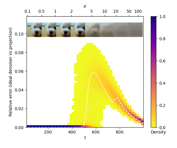
Figure 2: Ideal denoiser well-approximates projection onto the CIFAR-10 dataset. Dashed line plots error for the example shown, and density plot shows the error distribution over 10k different DDIM sampling trajectories.

In this section, we provide theoretical and empirical justifications for our relative error model, formally stated below:

Definition 3.1.

We say $\epsilon_{\theta}(x,\sigma)$ is an $(\eta,\nu)$-approximate projection if there exists constants $1>\eta\geq 0$ and $\nu\geq 1$ so that for all $x$ with unique ${\rm proj}_{\mathcal{K}}(x)$ and for all $\sigma$ satisfying $\frac{1}{\nu}{\rm dist}_{\mathcal{K}}(x)\leq\sqrt{n}\sigma\leq\nu{\rm dist}_{\mathcal{K}}(x)$, we have

$$\|x-\sigma\epsilon_{\theta}(x,\sigma)-{\rm proj}_{\mathcal{K}}(x)\|\leq\eta{\rm dist}_{\mathcal{K}}(x).$$

To justify this model, we will prove relative error bounds under different assumptions on $\epsilon_{\theta}$, $(x,\sigma)$ and $\mathcal{K}$. Analysis of DDIM based on this model is given in Section 4. Formal statements and proofs are deferred to Appendix B. Appendix E contains further experiments verifying our error model on image datasets.

3.1 Relative error under the manifold hypothesis

The manifold hypothesis [2, 11, 31] asserts that “real-world” datasets are (approximately) contained in low-dimensional manifolds of $\mathbb{R}^{n}$. Specifically, we suppose that $\mathcal{K}$ is a manifold of dimension $d$ with $d\ll n$. We next show that denoising is approximately equivalent to projection, when noise is small compared to the reach of $\mathcal{K}$, defined as the largest $\tau>0$ such that ${\rm proj}_{\mathcal{K}}(x)$ is unique when ${\rm dist}_{\mathcal{K}}(x)<\tau$.

The following classical result tells us that for small perturbations $w$, the difference between ${\rm proj}_{\mathcal{K}}(x_{0}+w)$ and $x_{0}$ is contained in the tangent space $\tan_{\mathcal{K}}(x_{0})$, a subspace of dimension $d$ associated with each $x_{0}\in\mathcal{K}$.

Lemma 3.1 (Theorem 4.8(12) in [10]).

Consider $x_{0}\in\mathcal{K}$ and $w\in\tan_{\mathcal{K}}(x_{0})^{\perp}$. If $\|w\|<\operatorname{reach}(\mathcal{K})$, then ${\rm proj}_{\mathcal{K}}(x_{0}+w)=x_{0}$.

When $n\gg d$, the orthogonal complement $\tan_{\mathcal{K}}(x)^{\perp}$ is large and will contain most of the weight of a random $\epsilon$, intuitively suggesting ${\rm proj}_{\mathcal{K}}(x_{0}+\sigma\epsilon)\approx x_{0}$ if $\sigma$ is small. In other words, we intuitively expect that the oracle denoiser, which returns $x_{0}$ given $x_{0}+\sigma\epsilon$, approximates projection.

We formalize this intuition using Gaussian concentration inequalities [45] and Lipschitz continuity of ${\rm proj}_{\mathcal{K}}(x)$ when ${\rm dist}_{\mathcal{K}}(x)<\operatorname{reach}(\mathcal{K})$.

Proposition 3.1 (Oracle denoising (informal)).

Given $x_{0}\in\mathcal{K}$, $\sigma>0$ and $\epsilon\sim\mathcal{N}(0,I)$, let $x_{\sigma}=x_{0}+\sigma\epsilon\in\mathbb{R}^{n}$. If $n\gg d$ and $\sigma\sqrt{n}\lesssim\operatorname{reach}(\mathcal{K})$, then with high probability,

$$\textstyle\left\lVert{\rm proj}_{\mathcal{K}}(x_{\sigma})-x_{0}\right\lVert\lesssim\sqrt{\frac{d}{n}}{\rm dist}_{\mathcal{K}}(x_{\sigma})$$

and for $\nu\lesssim 1+\sqrt{\frac{d}{n}}$, $\frac{1}{\nu}{\rm dist}_{\mathcal{K}}(x_{\sigma})\leq\sqrt{n}\sigma\leq\nu{\rm dist}_{\mathcal{K}}(x_{\sigma})$.

Observe this motivates both constants $\eta$ and $\nu$ used by our relative error model. We note prior analysis of diffusion under the manifold hypothesis is given by [7].

3.2 Relative error in large noise regime

We next analyze denoisers in the large-noise regime, when ${\rm dist}_{\mathcal{K}}(x)$ is much larger than $\operatorname{diam}(\mathcal{K}):=\sup\{\|x-y\|:x,y\in\mathcal{K}\}$. In this regime (see Figure 1(b) for an illustration), any denoiser that predicts a point in the convex hull of $\mathcal{K}$ approximates projection with error small compared to ${\rm dist}_{\mathcal{K}}(x)$.

Proposition 3.2.

Suppose $x-\sigma\epsilon_{\theta}(x,\sigma)\in\operatorname*{convhull}(\mathcal{K})$. If $\sqrt{n}\sigma\leq\nu{\rm dist}_{\mathcal{K}}(x)$, then $\left\lVert x-\sigma\epsilon_{\theta}(x,\sigma)-{\rm proj}_{\mathcal{K}}(x)\right\lVert\leq\nu\frac{\operatorname{diam}(\mathcal{K})}{\sqrt{n}\sigma}{\rm dist}_{\mathcal{K}}(x)$.

Thus any denoiser that predicts any weighted mean of the data, for instance the ideal denoiser, well approximates projection when $\sqrt{n}\sigma\gg\operatorname{diam}(\mathcal{K})$. For most pixel-space diffusion models used in practice, $\sqrt{n}\sigma_{N}$ is usually 50-100 times the diameter of the training set, with $\sqrt{n}\sigma_{t}$ in this regime for a significant proportion of timesteps.

3.3 Relative error of ideal denoisers

We now consider the case where $\mathcal{K}$ is a finite set and $\epsilon_{\theta}(x,\sigma)$ is the ideal denoiser $\epsilon^{*}(x,\sigma)$. We first show that predicting $\hat{x}_{0}$ with the ideal denoiser is equivalent to projection using the $\sigma$-smoothed distance function:

Proposition 3.3.

For all $\sigma>0$ and $x\in\mathbb{R}^{n}$, we have

$$\nabla_{x}{\textstyle\frac{1}{2}}\operatorname{dist}^{2}_{\mathcal{K}}(x,\sigma)=\sigma\epsilon^{*}(x,\sigma).$$

This shows our relative error model is in fact a bound on

$$\|\nabla_{x}\operatorname{dist}^{2}_{\mathcal{K}}(x,\sigma)-\nabla_{x}\operatorname{dist}^{2}_{\mathcal{K}}(x)\|,$$

the error between the gradient of the smoothed distance function and that of the true distance function. Since the amount of smoothing is directly determined by $\sigma$, it is therefore natural to bound this error using ${\rm dist}_{\mathcal{K}}(x)$ when $\sqrt{n}\sigma\approx{\rm dist}_{\mathcal{K}}(x)$. In other words, 3.3 directly motivates our error-model.

Towards a rigorous bound, let $N_{\alpha}(x)$ denote the subset of $x_{0}\in\mathcal{K}$ satisfying $\left\lVert x-x_{0}\right\lVert\leq\alpha{\rm dist}_{\mathcal{K}}(x)$ for $\alpha\geq 1$. Consider the following.

Proposition 3.4.

If $\alpha\geq 1+\frac{2\nu^{2}}{n}\left(\frac{1}{e}+\log\left(\frac{\left|\mathcal{K}\right|}{\eta}\right)\right)$ and $\frac{1}{\nu}{\rm dist}_{\mathcal{K}}(x)\leq\sqrt{n}\sigma$, then

$$\left\lVert x-\sigma\epsilon^{*}(x,\sigma)-{\rm proj}_{\mathcal{K}}(x)\right\lVert\leq\eta{\rm dist}_{\mathcal{K}}(x)+C_{x,\alpha}$$

where $C_{x,\alpha}:=\sup_{x_{0}\in N_{\alpha}}\|x_{0}-{\rm proj}_{\mathcal{K}}(x)\|$.

We can guarantee $C_{x,\alpha}$ is zero when ${\rm dist}_{\mathcal{K}}(x)$ is small compared to the minimum pairwise distance of points in $\mathcal{K}$. Combined with 3.2, this shows the ideal denoiser has low relative error in both the large and small noise regimes. We cannot guarantee that $C_{x,\alpha}$ is small relative to ${\rm dist}_{\mathcal{K}}(x)$ in all regimes, however, due to pathological cases, e.g., $x$ is exactly between two points in $N_{\alpha}$. Nevertheless, Figure 2 empirically shows that the relative error of the ideal denoiser $\left\lVert x_{t}-\sigma\epsilon^{*}(x,\sigma_{t})-{\rm proj}_{\mathcal{K}}(x_{t})\right\lVert/{\rm dist}_{\mathcal{K}}(x_{t})$ is small at all pairs $(x_{t},\sigma_{t})$ generated by the DDIM sampler, suggesting these pathologies do not appear in practice.

4 Gradient Descent Analysis of Sampling

Having justified the relative error model in Section 3, we now use it to study the DDIM sampler. As a warmup, we first consider the limiting case of zero error, where we see DDIM is precisely gradient descent on the squared-distance function with step-size determined by $\sigma_{t}$. We then generalize this result to arbitrary $(\eta,\nu)$, showing DDIM is equivalent to gradient-descent with relative error. Proofs are postponed to Appendix C.

4.1 Exact Projection and Gradient Descent

We state our zero-error assumption in terms of the error-model as follows.

Assumption 1.

$\epsilon_{\theta}$ is a $(0,1)$-approximate projection.

We can now characterize DDIM as follows.

Theorem 4.1.

Let $x_{N},\ldots,x_{0}$ denote a sequence (5) generated by DDIM on a schedule $\left\{\sigma_{t}\right\}_{t=N}^{0}$ and $f(x):=\frac{1}{2}{\rm dist}_{\mathcal{K}}(x)^{2}$. Suppose that 1 holds, $\nabla f(x_{t})$ exists for all $t$ and ${\rm dist}_{\mathcal{K}}(x_{N})=\sqrt{n}\sigma_{N}$. Then $x_{t}$ is a sequence generated by gradient descent with step-size $\beta_{t}:=1-\sigma_{t-1}/\sigma_{t}$:

$$x_{t-1}=x_{t}-\beta_{t}\nabla f(x_{t}),$$

and ${\rm dist}_{\mathcal{K}}(x_{t})=\sqrt{n}\sigma_{t}$ for all $t$.

We remark that the existence of $\nabla f(x_{t})$ is a weak assumption as it is generically satisfied by almost all $x\in\mathbb{R}^{n}$.

4.2 Approximate Projection and Gradient Descent with Error

We next establish upper and lower-bounds of distance under approximate gradient descent iterations. Given $\left\{\sigma_{t}\right\}_{t=N}^{0}$, let $\beta_{t}:=1-\sigma_{t-1}/\sigma_{t}$ and

$$L_{t}^{\sigma,\eta}:=\prod^{N}_{i=t}(1-\beta_{i}(\eta+1)),U_{t}^{\sigma,\eta}:=\prod^{N}_{i=t}(1+\beta_{i}(\eta-1)).$$

Lemma 4.1.

For $\mathcal{K}\subseteq\mathbb{R}^{n}$, let $f(x):=\frac{1}{2}{\rm dist}_{\mathcal{K}}(x)^{2}$. If $x_{t-1}=x_{t}-\beta_{t}(\nabla f(x_{t})+e_{t})$ for $e_{t}$ satisfying $\|e_{t}\|\leq\eta{\rm dist}_{\mathcal{K}}(x_{t})$ and $0\leq\beta_{t}\leq 1$, then

$$L_{t}^{\sigma,\eta}{\rm dist}_{\mathcal{K}}(x_{N})\leq{\rm dist}_{\mathcal{K}}(x_{t-1})\leq U_{t}^{\sigma,\eta}{\rm dist}_{\mathcal{K}}(x_{N}).$$

Observe that the distance upper bound decreases only if $\beta_{i}<1$ when $\eta>0$. This conforms with our intuition that step sizes are limited by the error in our gradient estimates.

The challenge in applying 4.1 to DDIM lies in the specifics of our relative error model, which states that $\epsilon_{\theta}(x_{t},\sigma_{t})$ provides an $\eta$-accurate estimate of $\nabla f(x_{t})$ only if $\sigma_{t}$ provides a $\nu$-accurate estimate of ${\rm dist}_{\mathcal{K}}(x_{t})$. Hence we must first control the difference between $\sigma_{t}$ and distance ${\rm dist}_{\mathcal{K}}(x_{t})$ by imposing the following conditions on $\sigma_{t}$.

Definition 4.1.

We say that parameters $\left\{\sigma_{t}\right\}_{t=N}^{0}$ are $(\eta,\nu)$-admissible if, for all $t\in\{1,\ldots,N\}$,

$$\textstyle\frac{1}{\nu}U_{t}^{\sigma,\eta}\leq\prod^{N}_{i=t}(1-\beta_{i})\leq\nu L_{t}^{\sigma,\eta}.$$ (8)

Intuitively, an admissible schedule decreases $\sigma_{t}$ slow enough (corresponding to taking smaller gradient steps) to ensure $\frac{1}{\nu}{\rm dist}_{\mathcal{K}}(x_{t})\leq\sqrt{n}\sigma_{t}\leq\nu{\rm dist}_{\mathcal{K}}(x_{t})$ holds at each iteration. Our analysis assumes admissibility of the noise schedule and our relative-error model (3.1):

Assumption 2.

For $\eta>0$ and $\nu\geq 1$, $\left\{\sigma_{t}\right\}_{t=N}^{0}$ is $(\eta,\nu)$-admissible and $\epsilon_{\theta}$ is an $(\eta,\nu)$-approximate projection.

Our main result follows. In simple terms, it states that DDIM is approximate gradient descent, that admissible schedules $\sigma_{t}$ are good estimates of distance, and that the error bounds of 4.1 hold.

Theorem 4.2 (DDIM with relative error).

Let 2 hold. Let $x_{t}$ denote the sequence generated by DDIM and suppose that the gradient of $f(x):=\frac{1}{2}{\rm dist}_{\mathcal{K}}(x)^{2}$ exists for all $x_{t}$. Suppose also that ${\rm dist}_{\mathcal{K}}(x_{N})=\sqrt{n}\sigma_{N}$. Then:

• $x_{t}$ is generated by approximate gradient descent iterations of the form in 4.1 with $\beta_{t}=1-\sigma_{t-1}/\sigma_{t}$.

• $\frac{1}{\nu}{\rm dist}_{\mathcal{K}}(x_{t})\leq\sqrt{n}\sigma_{t}\leq\nu{\rm dist}_{\mathcal{K}}(x_{t})$ for all $t$.

• ${\rm dist}_{\mathcal{K}}(x_{N})L_{t}^{\sigma,\eta}\leq{\rm dist}_{\mathcal{K}}(x_{t-1})\leq{\rm dist}_{\mathcal{K}}(x_{N})U_{t}^{\sigma,\eta}$

4.3 Admissible Log-Linear Schedules for DDIM

We next characterize admissible $\sigma_{t}$ of the form $\sigma_{t-1}=(1-\beta)\sigma_{t}$ where $\beta$ denotes a constant step-size. This illustrates that admissible $\sigma_{t}$-sequences not only exist, they can also be explicitly constructed from $(\eta,\nu)$.

Theorem 4.3.

Fix $\beta\in\mathbb{R}$ satisfying $0\leq\beta<1$ and suppose that $\sigma_{t-1}=(1-\beta)\sigma_{t}$. Then $\sigma_{t}$ is $(\eta,\nu)$-admissible if and only if $\beta\leq\beta_{*,N}$ where $\beta_{*,N}:=\frac{c}{\eta+c}$ for $c:=1-\nu^{-1/N}$.

Suppose we fix $(\eta,\nu)$ and choose, for a given $N$, the step-size $\beta_{*,N}$. It is natural to ask how the error bounds of 4.2 change as $N$ increases. We establish the limiting behavior of the final output $(\sigma_{0},x_{0})$ of DDIM.

Theorem 4.4.

Let $x_{N},\ldots,x_{1},x_{0}$ denote the sequence generated by DDIM with $\sigma_{t}$ satisfying $\sigma_{t-1}=(1-\beta_{*,N})\sigma_{t}$ for $\nu\geq 1$ and $\eta>0$. Then

• $\raisebox{2.15277pt}{\scalebox{0.8}{$\displaystyle\lim_{N\rightarrow\infty}\;$}}\frac{\sigma_{0}}{\sigma_{N}}=\raisebox{2.15277pt}{\scalebox{0.8}{$\displaystyle\lim_{N\rightarrow\infty}\;$}}(1-\beta_{*,N})^{N}=\nu^{-1/\eta}$.

• $\raisebox{2.15277pt}{\scalebox{0.8}{$\displaystyle\lim_{N\rightarrow\infty}\;$}}\frac{{\rm dist}_{\mathcal{K}}(x_{0})}{{\rm dist}_{\mathcal{K}}(x_{N})}\leq\raisebox{2.15277pt}{\scalebox{0.8}{$\displaystyle\lim_{N\rightarrow\infty}\;$}}(1+(\eta-1)\beta_{*,N})^{N}=\nu^{\frac{\eta-1}{\eta}}$.

This theorem illustrates that final error, while bounded, need not converge to zero under our error model. This motivates heuristically updating the step-size from $\beta_{*,N}$ to a full step $(\beta=1)$ during the final DDIM iteration. We adopt this approach in our experiments (Section 6).

Algorithm 1 DDIM sampler [40]

$(\sigma_{N},\ldots,\sigma_{0})$, $x_{N}\sim\mathcal{N}(0,I)$, $\epsilon_{\theta}$

Compute $x_{0}$ with $N$ evaluations of $\epsilon_{\theta}$

for $t=N,\ldots,1$ do

     $x_{t-1}\leftarrow x_{t}+(\sigma_{t-1}-\sigma_{t})\epsilon_{\theta}(x_{t},\sigma_{t})$

return $x_{0}$

Algorithm 2 Our gradient estimation sampler

$(\sigma_{N},\ldots,\sigma_{0})$, $x_{N}\sim\mathcal{N}(0,I)$, $\epsilon_{\theta}$

Compute $x_{0}$ with $N$ evaluations of $\epsilon_{\theta}$

$x_{N-1}\leftarrow x_{N}+(\sigma_{N-1}-\sigma_{N})\epsilon_{\theta}(x_{N},\sigma_{N})$

for $t=N-1,\ldots,1$ do

     $\bar{\epsilon}_{t}\leftarrow 2\epsilon_{\theta}(x_{t},\sigma_{t})-\epsilon_{\theta}(x_{t+1},\sigma_{t+1})$

     $x_{t-1}\leftarrow x_{t}+(\sigma_{t-1}-\sigma_{t})\bar{\epsilon}_{t}$

return $x_{0}$

5 Improving Deterministic Sampling Algorithms via Gradient Estimation

Figure 3: Illustration of our choice of $\bar{\epsilon}_{t}$

Section 3 establishes that $\epsilon_{\theta}(x,\sigma)\approx\sqrt{n}\nabla{\rm dist}_{\mathcal{K}}(x)$ when ${\rm dist}_{\mathcal{K}}(x)\approx\sqrt{n}\sigma$. We next exploit an invariant property of $\nabla{\rm dist}_{\mathcal{K}}(x)$ to reduce the prediction error of $\epsilon_{\theta}$ via gradient estimation.

The gradient $\nabla{\rm dist}_{\mathcal{K}}(x)$ is invariant along line segments between a point $x$ and its projection ${\rm proj}_{\mathcal{K}}(x)$, i.e., letting $\hat{x}={\rm proj}_{\mathcal{K}}(x)$, for all $\theta\in(0,1]$ we have

$$\nabla{\rm dist}_{\mathcal{K}}(\theta x+(1-\theta)\hat{x})=\nabla{\rm dist}_{\mathcal{K}}(x).$$ (9)

Hence, $\epsilon_{\theta}(x,\sigma)$ should be (approximately) constant on this line-segment under our assumption that $\epsilon_{\theta}(x,\sigma)\approx\sqrt{n}\nabla{\rm dist}_{\mathcal{K}}(x)$ when ${\rm dist}_{\mathcal{K}}(x)\approx\sqrt{n}\sigma$. Precisely, for $x_{1}$ and $x_{2}$ on this line-segment, we should have

$$\epsilon_{\theta}(x_{1},\sigma_{t_{1}})\approx\epsilon_{\theta}(x_{2},\sigma_{t_{2}})$$ (10)

if $t_{i}$ satisfies ${\rm dist}_{\mathcal{K}}(x_{i})\approx\sqrt{n}\sigma_{t_{i}}$. This property suggests combining previous denoiser outputs $\{\epsilon_{\theta}(x_{i},\sigma_{i})\}^{N}_{i=t+1}$ to estimate $\epsilon_{t}:=\sqrt{n}\nabla{\rm dist}_{\mathcal{K}}(x_{t})$. We next propose a practical second-order method for this estimation that combines the current denoiser output with the previous. Recently introduced consistency models [41] penalize violation of (10) during training. Interpreting denoiser output as $\nabla{\rm dist}_{\mathcal{K}}(x)$ and invoking (9) offers an alternative justification for these models.

Let $e_{t}(\epsilon_{t})=\epsilon_{t}-\epsilon_{\theta}(x_{t},\sigma_{t})$ be the error of $\epsilon_{\theta}(x_{t},\sigma_{t})$ when predicting $\epsilon_{t}$. To estimate $\epsilon_{t}$ from $\epsilon_{\theta}(x_{t},\sigma_{t})$, we minimize the norm of this error concatenated over two time-steps. Precisely, letting $y_{t}(\epsilon)=(e_{t}(\epsilon),e_{t+1}(\epsilon))$, we compute

$$\bar{\epsilon}_{t}:=\operatorname*{arg\,min}_{\epsilon}\left\lVert y_{t}(\epsilon)\right\lVert^{2}_{W},$$ (11)

where $W$ is a specified positive-definite weighting matrix. In Appendix D we show that this error model, for a particular family of weight matrices, results in the update rule

$$\bar{\epsilon}_{t}=\gamma\epsilon_{\theta}(x_{t},\sigma_{t})+(1-\gamma)\epsilon_{\theta}(x_{t+1},\sigma_{t+1}),$$ (12)

where we can search over $W$ by searching over $\gamma$.

6 Experiments

Ours	UniPC	DPM++	PNDM	DDIM
	[49]	[26]	[22]	[40]
FID 13.77	15.59	15.43	19.43	14.06

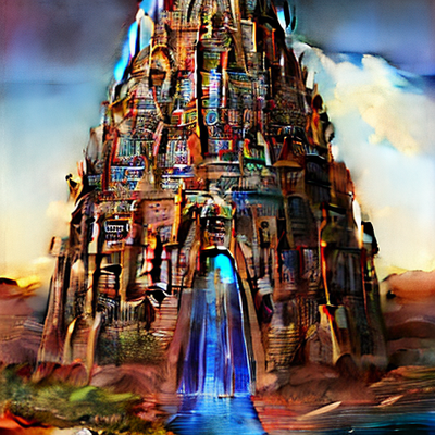
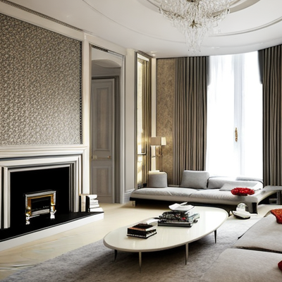
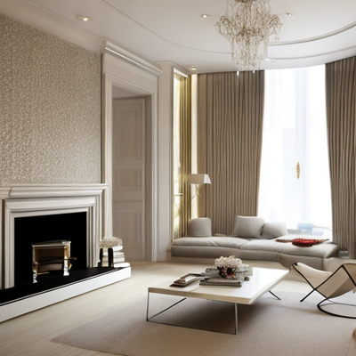
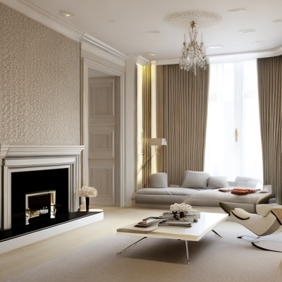
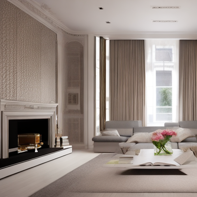
Figure 4: Outputs of our sampler on text-to-image Stable Diffusion compared to other commonly used samplers, when limited to $N=10$ function evaluations. We also report FID scores for text-to-image generation on MS-COCO 30K.

We evaluate modifications of DDIM (Algorithm 1) that leverage insights from Section 5 and Section 4.3. Following Section 5 we modify DDIM to use a second-order update that corrects for error in the denoiser output (Algorithm 2). Specifically, we use the Equation 12 update with $\gamma=2$, which is empirically tuned (see Appendix E). A comparison of this update with DDIM is visualized in Figure 3. Following Section 4.3, we select a noise schedule $(\sigma_{N},\ldots,\sigma_{0})$ that decreases at a log-linear (geometric) rate. The specific rate is determined by an initial and target noise level. Our $\sigma_{t}$ schedule is illustrated in Figure 5, along with other commonly used schedules. We note that log-linear schedules have been previously proposed for SDE-samplers [43]; to our knowledge we are the first to propose and analyze their use for DDIM. All the experiments were run on a single Nvidia RTX 4090 GPU.

6.1 Evaluation of Noise Schedule

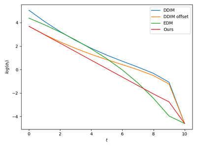
Figure 5: Plot of different choices of $\log(\sigma_{t})$ for $N=10$.

Schedule	CIFAR-10	CelebA
DDIM	16.86	18.08
DDIM Offset	14.18	15.38
EDM	20.85	16.72
Ours	13.25	13.55

Table 1: FID scores of the DDIM sampler (Algorithm 1) with different $\sigma_{t}$ schedules on the CIFAR-10 model for $N=10$ steps.

In Figure 5 we plot our schedule (with our choices of $\sigma_{t}$ detailed in Appendix F) with three other commonly used schedules on a log scale. The first is the evenly spaced subsampling of the training noise levels used by DDIM. The second “DDIM Offset” uses the same even spacing but starts at a smaller $\sigma_{N}$, the same as that in our schedule. This type of schedule is typically used for guided image generation such as SDEdit [27]. The third “EDM” is the schedule used in [15, Eq. 5], with $\sigma_{\max}=80,\sigma_{\min}=0.002$ and $\rho=7$.

We then test these schedules on the DDIM sampler Algorithm 1 by sampling images with $N=10$ steps from the CIFAR-10 and CelebA models. We see that in Table 1 that our schedule improves the FID of the DDIM sampler on both datasets even without the second-order updates. This is in part due to choosing a smaller $\sigma_{N}$ so the small number of steps can be better spent on lower noise levels (the difference between “DDIM” and “DDIM Offset”), and also because our schedule decreases $\sigma_{t}$ at a faster rate than DDIM (the difference between “DDIM Offset” and “Ours”).

6.2 Evaluation of Full Sampler

	CIFAR-10 FID				CelebA FID
Sampler	$N=5$	$N=10$	$N=20$	$N=50$	$N=5$	$N=10$	$N=20$	$N=50$
Ours	12.53	3.85	3.39	3.43	10.73	4.30	3.56	3.78
DDIM [40]	47.20	16.86	8.28	4.81	32.21	18.08	11.81	7.39
PNDM [22]	13.9	7.03	5.00	3.95	11.3	7.71	5.51	3.34
DPM [25]		6.37	3.72	3.48		5.83	2.82	2.71
DEIS [48]	18.43	7.12	4.53	3.78	25.07	6.95	3.41	2.95
UniPC [49]	23.22	3.87
A-DDIM [1]		14.00	5.81*	4.04		15.62	9.22*	6.13

Table 2: FID scores of our sampler compared to that of other samplers for pretrained CIFAR-10 and CelebA models with a discrete linear schedule. The first half of the table shows our computational results whereas the second half of the table show results taken from the respective papers. *Results for $N=25$

We quantitatively evaluate our sampler (Algorithm 2) by computing the Fréchet inception distance (FID) [12] between all the training images and 50k generated images. We use denoisers from [13, 40] that were pretrained on the CIFAR-10 (32x32) and CelebA (64x64) datasets [18, 24]. We compare our results with other samplers using the same denoisers. The FID scores are tabulated in Table 2, showing that our sampler achieves better performance on both CIFAR-10 (for $N=5,10,20,50$) and CelebA (for $N=5,10$).

We also incorporated our sampler into Stable Diffusion (a latent diffusion model). We change the noise schedule $\sigma_{t}$ as described in Appendix F. In Figure 4, we show some example results for text to image generation in $N=10$ function evaluations, as well as FID results on 30k images generated from text captions drawn the MS COCO [21] validation set. From these experiments we can see that our sampler performs comparably to other commonly used samplers, but with the advantage of being much simpler to describe and implement.

7 Related Work and Discussion

Learning diffusion models

Diffusion was originally introduced as a variational inference method that learns to reverse a noising process [39]. This approach was empirically improved by [13, 28] by introducing the training loss (2), which is different from the original variational lower bound. This improvement is justified from the perspective of denoising score matching [42, 43], where the $\epsilon_{\theta}$ is interpreted as $\nabla\log(p(x_{t},\sigma_{t}))$, the gradient of the log density of the data distribution perturbed by noise. Score matching is also shown to be equivalent to denoising autoencoders with Gaussian noise [46].

Sampling from diffusion models

Samplers for diffusion models started with probabilistic methods (e.g. [13]) that formed the reverse process by conditioning on the denoiser output at each step. In parallel, score based models [42, 43] interpret the forward noising process as a stochastic differential equation (SDE), so SDE solvers based on Langevian dynamics [47] are employed to reverse this process. As models get larger, computational constraints motivated the development of more efficient samplers. [40] then discovered that for smaller number of sampling steps, deterministic samplers perform better than stochastic ones. These deterministic samplers are constructed by reversing a non-Markovian process that leads to the same training objective, which is equivalent to turning the SDE into an ordinary differential equation (ODE) that matches its marginals at each sampling step.

This led to a large body of work focused on developing ODE and SDE solvers for fast sampling of diffusion models, a few of which we have evaluated in Table 2. Most notably, [15] put existing samplers into a common framework and isolated components that can be independently improved. Our sampler Algorithm 2 bears most similarity to linear multistep methods, which can also be interpreted as accelerated gradient descent [36]. What differs is the error model: ODE solvers aim to minimize discretization error whereas we aim to minimize gradient estimation error, resulting in different “optimal” samplers.

Linear-inverse problems and conditioning

Several authors [14, 6, 16] have devised samplers for finding images that satisfy linear equations $Ax=b$. Such linear inverse problems generalize inpainting, colorization, and compressed sensing. In our framework, we can interpret this samplers as algorithms for equality constraint minimization of the distance function, a classical problem in optimization. Similarly, the widely used technique of conditioning [9] can be interpreted as multi-objective optimization, where minimization of distance is replaced with minimization of ${\rm dist}_{\mathcal{K}}(x)^{2}+g(x)$ for an auxiliary objective function $g(x)$.

Score distillation sampling

We illustrate the potential of our framework for discovering new applications of diffusion models by deriving Score Distillation Sampling (SDS), a method for parameterized optimization introduced in [30] in the context of text to 3D object generation. At a high-level, this technique finds $(x,\theta)$ satisfying non-linear equations $x=g(\theta)$ subject to the constraint $x\in\mathcal{K}$, where $\mathcal{K}$ denotes the image manifold. It does this by iteratively updating $x$ with a direction proportional to $(\epsilon_{\theta}(x+\sigma\epsilon,\sigma)-\epsilon)\nabla g(\theta)$, where $\sigma$ is a randomly chosen noise level and $\epsilon\sim\mathcal{N}(0,I)$. Under our framework, this iteration can be interpreted as gradient descent on the squared distance function with gradient $\frac{1}{2}\nabla_{\theta}{\rm dist}_{\mathcal{K}}(g(\theta))^{2}=(x-{\rm proj}_{\mathcal{K}}(x))\nabla g(\theta)$, with the assumption that ${\rm proj}_{\mathcal{K}}(x)\approx{\rm proj}_{\mathcal{K}}(x+\sigma\epsilon)$, along with our Section 3 denoising approximation ${\rm proj}_{\mathcal{K}}(x+\sigma\epsilon)\approx x+\sigma\epsilon-\sigma\epsilon_{\theta}(x+\sigma\epsilon,\sigma)$.

Learning the distance function

Reinterpreting denoising as projection, or equivalently gradient descent on the distance function, has a few immediate implications. First, it suggests generalizations that draw upon the literature for computing distance functions and projection operators. Such techniques include Fast Marching Methods [37], kd-trees, and neural-network approaches, e.g., [29, 33]. Using concentration inequalities, we can also interpret training a denoiser as learning a solution to the Eikonal PDE, given by $\|\nabla d(x)\|=1$. Other techniques for solving this PDE with deep neural nets include [38, 20, 3].

8 Conclusion and Future Work

We have presented a simple framework for analyzing and generalizing diffusion models that has led to a new sampling approach and new interpretations of pre-existing techniques. Moreover, the key objects in our analysis —the distance function and the projection operator—are canonical objects in constrained optimization. We believe our work can lead to new generative models that incorporate sophisticated objectives and constraints for a variety of applications. We also believe this work can be leveraged to incorporate existing denoisers into optimization algorithms in a plug-in-play fashion, much like the work in [4, 19, 33].

Combining the multi-level noise paradigm of diffusion with distance function learning [29] is an interesting direction, as are diffusion-models that carry out projection using analytic formulae or simple optimization routines.

Appendix A Equivalent Definitions of DDIM and DDPM

The DDPM and DDIM samplers are usually described in a different coordinate system $z_{t}$ defined by parameters $\bar{\alpha}_{t}$ and the following relations , where the noise model is defined by a schedule $\bar{\alpha}_{t}$:

$$y\approx\sqrt{\bar{\alpha}_{t}}z+\sqrt{1-\bar{\alpha}_{t}}\epsilon,$$ (13)

with the estimate $\hat{z}_{0}^{t}:=\hat{z}_{0}(z_{t},t)$ given by

$$\hat{z}_{0}(y,t):=\frac{1}{\sqrt{\bar{\alpha}_{t}}}(y-\sqrt{1-\bar{\alpha}_{t}}\epsilon^{\prime}_{\theta}(y,t)).$$ (14)

We have the following conversion identities between the $x$ and $z$ coordinates:

$$x_{0}=z_{0},\quad x_{t}=z_{t}/\sqrt{\bar{\alpha}_{t}},\quad\sigma_{t}=\sqrt{\frac{1-\bar{\alpha}_{t}}{\bar{\alpha}_{t}}},\quad\epsilon_{\theta}(y,\sigma_{t})=\epsilon^{\prime}_{\theta}(y/\sqrt{\bar{\alpha}_{t}},t).$$ (15)

While this change-of-coordinates is used in [40, Section 4.3] and in [15]–and hence not new– we rigorously prove equivalence of the DDIM and DDPM samplers given in Section 2 with their original definitions.

DDPM

Given initial $z_{N}$, the DDPM sampler constructs the sequence

$$z_{t-1}=\frac{\sqrt{\bar{\alpha}_{t-1}}(1-\alpha_{t})}{1-\bar{\alpha}_{t}}\hat{z}^{t}_{0}+\frac{\sqrt{\alpha}_{t}(1-\bar{\alpha}_{t-1})}{1-\bar{\alpha}_{t}}z_{t}+\sqrt{\frac{1-\bar{\alpha}_{t-1}}{1-\bar{\alpha}_{t}}(1-\alpha_{t})}w_{t},$$ (16)

where $\alpha_{t}:=\bar{\alpha}_{t}/\bar{\alpha}_{t-1}$ and $w_{t}\sim\mathcal{N}(0,I)$. This is interpreted as sampling $z_{t-1}$ from a Gaussian distribution conditioned on $z_{t}$ and $\hat{z}_{0}^{t}$ [13].

Proposition A.1 (DDPM change of coordinates).

The sampling update (4) is equivalent to the update (16) under the change of coordinates (15).

Proof.

First we write (4) in terms of $z_{t}$, $\epsilon^{\prime}_{\theta}(z_{t},t)$ and $w_{t}$ using (14):

$$z_{t-1} =\frac{\sqrt{\bar{\alpha}_{t-1}}(1-\alpha_{t})}{\sqrt{\bar{\alpha}_{t}}(1-\bar{\alpha}_{t})}\left(z_{t}-\sqrt{1-\bar{\alpha}_{t}}\epsilon^{\prime}_{\theta}(z_{t},t)\right)+\frac{\sqrt{\alpha}_{t}(1-\bar{\alpha}_{t-1})}{1-\bar{\alpha}_{t}}z_{t}+\sqrt{\frac{1-\bar{\alpha}_{t-1}}{1-\bar{\alpha}_{t}}(1-\alpha_{t})}w_{t}$$

$$=\frac{z_{t}}{\sqrt{\alpha_{t}}}+\frac{\alpha_{t}-1}{\sqrt{\alpha_{t}(1-\bar{\alpha}_{t}))}}\epsilon^{\prime}_{\theta}(z_{t},t)+\sqrt{\frac{1-\bar{\alpha}_{t-1}}{1-\bar{\alpha}_{t}}(1-\alpha_{t})}w_{t}.$$

Next we divide both sides by $\sqrt{\bar{\alpha}_{t-1}}$ and change $z_{t}$ and $z_{t-1}$ to $x_{t}$ and $x_{t-1}$:

$$x_{t-1}=x_{t}+\frac{\alpha_{t}-1}{\sqrt{\bar{\alpha}_{t}(1-\bar{\alpha}_{t})}}\epsilon_{\theta}(x_{t},\sigma_{t})+\sqrt{\frac{1-\bar{\alpha}_{t-1}}{\bar{\alpha}_{t-1}}\frac{1-\alpha_{t}}{1-\bar{\alpha}_{t}}}w_{t}.$$

Now if we define

$$\eta :=\sqrt{\frac{1-\bar{\alpha}_{t-1}}{\bar{\alpha}_{t-1}}\frac{1-\alpha_{t}}{1-\bar{\alpha}_{t}}}=\sigma_{t-1}\sqrt{\frac{1-\bar{\alpha}_{t}/\bar{\alpha}_{t-1}}{1-\bar{\alpha}_{t}}},$$

$$\sigma_{t^{\prime}} :=\sqrt{\sigma_{t-1}^{2}-\eta^{2}}=\sigma_{t-1}\sqrt{\frac{\bar{\alpha}_{t}(1/\bar{\alpha}_{t-1}-1)}{1-\bar{\alpha}_{t}}}=\frac{\sigma_{t-1}^{2}}{\sigma_{t}},$$

it remains to check that

$$\sigma_{t^{\prime}}-\sigma_{t}=\frac{\sigma_{t-1}^{2}-\sigma_{t}^{2}}{\sigma_{t}}=\frac{1/\bar{\alpha}_{t-1}-1/\bar{\alpha}_{t}}{\sqrt{1-\bar{\alpha}_{t}}/\sqrt{\bar{\alpha}_{t}}}=\frac{\alpha_{t}-1}{\sqrt{\bar{\alpha}_{t}(1-\bar{\alpha}_{t})}}.$$

∎

DDIM

Given initial $z_{N}$, the DDIM sampler constructs the sequence

$$z_{t-1} =\sqrt{\bar{\alpha}_{t-1}}\hat{z}_{0}^{t}+\sqrt{1-\bar{\alpha}_{t-1}}\epsilon^{\prime}_{\theta}(z_{t},t),$$ (17)

i.e., it estimates $\hat{z}_{0}^{t}$ from $z_{t}$ and then constructs $z_{t-1}$ by simply updating $\bar{\alpha}_{t}$ to $\bar{\alpha}_{t-1}$. This sequence can be equivalently expressed in terms of $\hat{z}_{0}^{t}$ as

$$z_{t-1} =\sqrt{\bar{\alpha}_{t-1}}\hat{z}_{0}^{t}+\sqrt{\frac{1-\bar{\alpha}_{t-1}}{1-\bar{\alpha}_{t}}}(z_{t}-\sqrt{\bar{\alpha}_{t}}\hat{z}_{0}^{t}).$$ (18)

Proposition A.2 (DDIM change of coordinates).

The sampling update (5) is equivalent to the update (18) under the change of coordinates (15).

Proof.

First we write (17) in terms of $z_{t}$ and $\epsilon^{\prime}_{\theta}(z_{t},t)$ using (14):

$$z_{t-1}=\sqrt{\frac{\bar{\alpha}_{t-1}}{\bar{\alpha}_{t}}}z_{t}+\left(\sqrt{1-\bar{\alpha}_{t-1}}-\sqrt{\frac{\bar{\alpha}_{t-1}}{\bar{\alpha}_{t}}}\sqrt{1-\bar{\alpha}_{t}}\right)\epsilon^{\prime}_{\theta}(z_{t},t).$$

Next we divide both sides by $\sqrt{\bar{\alpha}_{t-1}}$ and change $z_{t}$ and $z_{t-1}$ to $x_{t}$ and $x_{t-1}$:

$$x_{t-1} =x_{t}+\left(\sqrt{\frac{1-\bar{\alpha}_{t-1}}{\bar{\alpha}_{t-1}}}-\sqrt{\frac{\bar{\alpha}_{t-1}}{1-\bar{\alpha}_{t}}}\right)\epsilon_{\theta}(x_{t},\sigma_{t})$$

$$=x_{t}+(\sigma_{t-1}-\sigma_{t})\epsilon_{\theta}(x_{t},\sigma_{t}).$$

∎

Appendix B Formal Comparison of Denoising and Projection

B.1 Proof of 3.1

First, we state the formal version of 3.1

Proposition B.1 (Oracle denoising).

Fix $\sigma>0$, $t>0$ and let $\kappa(t):=\sqrt{(\sqrt{d}+t)^{2}+(\sqrt{n-d}+t)^{2}}$. Given $x_{0}\in\mathcal{K}$ and $\epsilon\sim\mathcal{N}(0,I)$, let $x_{\sigma}=x_{0}+\sigma\epsilon$. Suppose that $\operatorname{reach}(\mathcal{K})>\sigma\kappa(t)$ and $\sqrt{n-d}-\sqrt{d}-2t>0$. Then, for an absolute constant $\alpha>0$, we have, with probability at least $(1-\exp(-\alpha t^{2}))^{2}$, that

$$\sigma(\sqrt{n-d}-\sqrt{d}-2t)\leq\operatorname*{dist}(x_{\sigma})\leq\sigma(\sqrt{n-d}+\sqrt{d}+2t)$$

and

$$\|{\rm proj}_{\mathcal{K}}(x_{\sigma})-x_{0}\|\leq\frac{C(t)(\sqrt{d}+t)}{\sqrt{n-d}-\sqrt{d}-2t}{\rm dist}_{\mathcal{K}}(x_{\sigma})$$

where $C(t):=\frac{\operatorname{reach}(\mathcal{K})}{\operatorname{reach}(\mathcal{K})-\sigma\kappa(t)}$.

Our proof uses local Lipschitz continuity of the projection operator, stated formally as follows.

Proposition B.2 (Theorem 6.2(vi), Chapter 6 of [8]).

Suppose $0<\operatorname{reach}(\mathcal{K})<\infty$. Consider $h>0$ and $x,y\in\mathbb{R}^{n}$ satisfying $0<h<\operatorname{reach}(\mathcal{K})$ and ${\rm dist}_{\mathcal{K}}(x)\leq h$ and ${\rm dist}_{\mathcal{K}}(y)\leq h$. Then the projection map satisfies $\|{\rm proj}_{\mathcal{K}}(y)-{\rm proj}_{\mathcal{K}}(x)\|\leq\frac{\operatorname{reach}(\mathcal{K})}{\operatorname{reach}(\mathcal{K})-h}\|y-x\|$.

We also use the following concentration inequalities.

Proposition B.3.

Let $w\sim\mathcal{N}(0,\sigma^{2}I_{n})$. Let $S$ be a fixed subspace of dimension $d$ and denote by $w_{S}$ and $w_{S^{\perp}}$ the projections onto $S$ and $S^{\perp}$ respectively. Then for an absolute constant $\alpha$, the following statements hold

• With probability at least $1-\exp(-\alpha t^{2})$,

  $$\sigma(\sqrt{n}-t)\leq\left\lVert w\right\lVert\leq\sigma(\sqrt{n}+t)$$

• With probability at least $(1-\exp(-\alpha t^{2}))^{2}$,

  $$\sigma(\sqrt{d}-t)\leq\left\lVert w_{S}\right\lVert\leq\sigma(\sqrt{d}+t),\qquad\sigma(\sqrt{n-d}-t)\leq\left\lVert w_{S^{\perp}}\right\lVert\leq\sigma(\sqrt{n-d}+t),$$

Proof.

The first statement is proved in  [[]page 44, Equation 3.3]vershynin2018high. For the second, let $B\in\mathbb{R}^{n\times d}$ denote an orthonormal basis for $S$ and define $y=B^{T}w$ Then $\|y\|=\|w_{S}\|$. Further, $y\sim\mathcal{N}(0,\sigma^{2}I_{d\times d})$ given that $\operatorname{cov}(y)=\sigma^{2}B^{T}B=\sigma^{2}I_{d\times d}$. Hence, the bounds on $\|w_{S}\|$ hold with probability at least $p:=1-\exp(-\alpha t^{2})$ given the first statement. By similar argument, the bounds on $\|w_{S^{\perp}}\|$ also hold with probability $p$. Since $w_{S}$ and $w_{S^{\perp}}$ are independent, we deduce that both sets of bounds simultaneously hold with probability at least $p^{2}$. ∎

To prove B.1, we decompose random noise $\sigma\epsilon$ as

$$\sigma\epsilon=w_{N}+w_{T}$$ (19)

for $w_{T}\in\tan_{\mathcal{K}}(x_{0})$ and $w_{N}\in\tan_{\mathcal{K}}(x_{0})^{\perp}$ and use 3.1. The proof follows.

Proof of B.1.

Let $p:=1-\exp(-\alpha t^{2})$. B.3 asserts that, with probability at least $p^{2}$,

$$\sigma(\sqrt{d}-t)\leq\left\lVert w_{T}\right\lVert\leq\sigma(\sqrt{d}+t),\qquad\sigma(\sqrt{n-d}-t)\leq\left\lVert w_{N}\right\lVert\leq\sigma(\sqrt{n-d}+t),$$ (20)

These inequalities imply the claimed bounds on ${\rm dist}_{\mathcal{K}}(x_{\sigma})$, given that

$$\|w_{N}\|-\|w_{T}\|\leq{\rm dist}_{\mathcal{K}}(x_{\sigma})\leq\|w_{N}\|+\|w_{T}\|$$

by C.2 and the fact $\operatorname*{dist}(x_{0}+w_{N})=\|w_{N}\|$ under the reach assumption and 3.1.

Using $\operatorname*{proj}(x_{0}+w_{N})=x_{0}$, we observe that

$$\|\operatorname*{proj}(x_{\sigma})-x_{0}\| =\|\operatorname*{proj}(x_{0}+w_{N}+w_{T})-x_{0}\|$$

$$=\|\operatorname*{proj}(x_{0}+w_{N})-x_{0}+\operatorname*{proj}(x_{0}+w_{N}+w_{T})-\operatorname*{proj}(x_{0}+w_{N})\|$$

$$=\|\operatorname*{proj}(x_{0}+w_{N})-\operatorname*{proj}(x_{0}+w_{N}+w_{T})\|$$

$$\leq C\|w_{T}\|$$

$$\leq C\sigma(\sqrt{d}+t)$$

where the second-to-last inequality comes from B.2 using the fact that $\operatorname{reach}(\mathcal{K})>w$ and the inequalities ${\rm dist}_{\mathcal{K}}(x_{0}+w_{N})=\|w_{N}\|\leq\|w\|$ and ${\rm dist}_{\mathcal{K}}(x_{0}+w_{N}+w_{T})\leq\|w\|$. The proof is completed by dividing by our lower bound of ${\rm dist}_{\mathcal{K}}(x_{\sigma})$.

∎

B.2 Proof of 3.3

First we derive an explicit expression for the ideal denoiser for a uniform distribution over a finite set.

Lemma B.1.

When $D$ is a discrete uniform distribution over a set $\mathcal{K}$, the ideal denoiser $\epsilon^{*}$ is given by

$$\epsilon^{*}(x_{\sigma},\sigma)=\frac{\sum_{x_{0}\in\mathcal{K}}(x_{\sigma}-x_{0})\exp(-\left\lVert x_{\sigma}-x_{0}\right\lVert^{2}/2\sigma^{2})}{\sigma\sum_{x_{0}\in\mathcal{K}}\exp(-\left\lVert x_{\sigma}-x_{0}\right\lVert^{2}/2\sigma^{2})}.$$

Proof.

Writing the loss explicitly as

$$\mathcal{L}_{\sigma}(\epsilon^{*})=\int\sum_{x_{0}\in\mathcal{K}}\frac{1}{\left|\mathcal{K}\right|\sigma\sqrt{2\pi}}\exp\left(-\frac{\left\lVert x_{\sigma}-x_{0}\right\lVert^{2}}{2\sigma^{2}}\right)\left\lVert(x_{\sigma}-x_{0})/\sigma-\epsilon^{*}(x_{\sigma},\sigma)\right\lVert^{2}d(x_{\sigma}),$$

It suffices to take the point-wise minima of the expression inside the integral, which is convex in terms of $\epsilon^{*}$. ∎

From this expression of the ideal denoiser $\epsilon^{*}$, we see that $\hat{x}_{0}$ can be written as a convex combination of points in $\mathcal{K}$:

$$\hat{x}_{0}(x,\sigma)=\sigma\epsilon^{*}(x,\sigma)-x=\sum_{x_{0}\in\mathcal{K}}w(x,x_{0})x_{0},$$

where $\sum_{x_{0}\in\mathcal{K}}w(x,x_{0})=1$.

By taking the gradient of the log-sum-exp function in the definition of $\operatorname{dist}^{2}_{\mathcal{K}}(x,\sigma)$ then applying B.1, it is clear that

$$\nabla_{x}{\textstyle\frac{1}{2}}\operatorname{dist}^{2}_{\mathcal{K}}(x,\sigma)=\sigma\epsilon^{*}(x,\sigma).$$

B.3 Proof of 3.4

We wish to bound the error between the gradient of the true distance function and the result of the ideal denoiser. Precisely, we want to upper-bound the following in terms of $\operatorname{dist}_{\mathcal{K}}(x)=\left\lVert x-x_{0}^{*}\right\lVert$, where $x_{0}^{*}={\rm proj}_{\mathcal{K}}(x)$. We first define

$$w(x,x^{\prime}):=\frac{\exp(-\left\lVert x-x^{\prime}\right\lVert^{2}/2\sigma^{2})}{\sum_{x_{0}\in\mathcal{K}}\exp(-\left\lVert x-x_{0}\right\lVert^{2}/2\sigma^{2})}.$$

Note that by definition, we have $\sum_{x_{0}\in\mathcal{K}}w(x,x_{0})=1$. Letting $\bar{N}_{\alpha}$ denote the complement of $N_{\alpha}$ in $\mathcal{K}$, we have

$$\left\lVert\nabla{\textstyle\frac{1}{2}}\operatorname{dist}_{\mathcal{K}}(x)^{2}-\sigma\epsilon^{*}(x,\sigma)\right\lVert =\left\lVert\nabla{\textstyle\frac{1}{2}}\operatorname{dist}_{\mathcal{K}}(x)^{2}-\nabla{\textstyle\frac{1}{2}}\operatorname{dist}^{2}_{\mathcal{K}}(x,\sigma)\right\lVert$$

$$=\textstyle{\left\lVert x_{0}^{*}-\sum_{x_{0}\in\mathcal{K}}w(x,x_{0})x_{0}\right\lVert}$$

$$=\textstyle{\left\lVert\sum_{x_{0}\in\mathcal{K}}w(x,x_{0})(x^{*}_{0}-x_{0})\right\lVert}$$

$$\leq\|\sum_{x_{0}\in\bar{N}_{\alpha}}w(x,x_{0})(x^{*}_{0}-x_{0})\|+\|\sum_{x_{0}\in N_{\alpha}}w(x,x_{0})(x^{*}_{0}-x_{0})\|$$

$$\leq\|\sum_{x_{0}\in\bar{N}_{\alpha}}w(x,x_{0})(x^{*}_{0}-x_{0})\|+C_{x,\alpha}$$

The claim then follows from the following theorem.

Theorem B.1.

Suppose $\mathcal{K}$ is a finite-set and let $x_{0}^{*}={\rm proj}_{\mathcal{K}}(x)$. Suppose we have

$$\alpha\geq 1+\frac{2\sigma^{2}}{{\rm dist}_{\mathcal{K}}(x)^{2}}\left(\frac{1}{e}+\log\left(\frac{m}{\eta}\right)\right),$$ (21)

then $\textstyle\left\lVert\sum_{x_{0}\in\bar{N}_{\alpha}}w(x,x_{0})(x_{0}^{*}-x_{0})\right\lVert\leq\eta{\rm dist}_{\mathcal{K}}(x)$.

Proof.

Applying the triangle inequality, it suffices to upper-bound each of $w(x,x_{0})\left\lVert x_{0}^{*}-x_{0}\right\lVert$. For convenience of notation let $\delta(x_{0}):=\left\lVert x-x_{0}\right\lVert/\left\lVert x-x_{0}^{*}\right\lVert$. Note that by construction $\delta(x_{0})\geq 1$ for all $x_{0}\in\mathcal{K}$, and $\delta(x_{0})\geq\alpha$ for all $x_{0}\in\bar{N}_{\alpha}$. Then

$$\left\lVert x_{0}^{*}-x_{0}\right\lVert \leq\left\lVert x_{0}^{*}-x\right\lVert+\left\lVert x-x_{0}\right\lVert=(1+\delta(x_{0}))\left\lVert x-x_{0}^{*}\right\lVert,$$

$$w(x,x_{0}) \leq\exp\left(-\frac{\left\lVert x-x_{0}\right\lVert^{2}-\left\lVert x-x_{0}^{*}\right\lVert^{2}}{2\sigma^{2}}\right)\leq\exp\left(-\frac{(\delta(x_{0})^{2}-1)\left\lVert x-x_{0}^{*}\right\lVert^{2}}{2\sigma^{2}}\right).$$

From (21) and the fact that $1/e\geq\log(a)/a$ for $a=\delta(x_{0})+1\geq 1$, we have

$$\delta(x_{0})-1 \geq\alpha-1\geq\frac{2\sigma^{2}}{a\left\lVert x-x_{0}^{*}\right\lVert^{2}}\left(\log(a)+\log\left(\frac{m}{\epsilon}\right)\right)=\frac{2\sigma^{2}}{(\delta(x_{0})+1)\left\lVert x-x_{0}^{*}\right\lVert^{2}}\log\left(\frac{m(\delta(x_{0})+1)}{\epsilon}\right)$$

$$\delta(x_{0})^{2}-1 \geq\frac{2\sigma^{2}}{\left\lVert x-x_{0}^{*}\right\lVert^{2}}\log\left(\frac{m(\delta(x_{0})+1)}{\epsilon}\right)$$

Putting these together, we have:

$${\textstyle\left\lVert\sum_{x_{0}\in\bar{N}_{\alpha}}w(x,x_{0})(x_{0}^{*}-x_{0})\right\lVert} \leq\sum_{x_{0}\in\bar{N}_{\alpha}}(1+\delta(x_{0}))\left\lVert x-x_{0}^{*}\right\lVert\exp\left(-\frac{(\delta(x_{0})^{2}-1)\left\lVert x-x_{0}^{*}\right\lVert^{2}}{2\sigma^{2}}\right)$$

$$\leq\sum_{x_{0}\in\bar{N}_{\alpha}}\frac{\epsilon\left\lVert x-x_{0}^{*}\right\lVert}{m}$$

$$\leq\epsilon{\rm dist}_{\mathcal{K}}(x)$$

∎

Appendix C DDIM with Projection Error Analysis

C.1 Proof of 4.1

We use the following lemma for gradient descent applied to the squared-distance function $f(x)$.

Lemma C.1.

Fix $x\in\mathbb{R}^{n}$ and suppose that $\nabla f(x)$ exists. For step-size $0<\beta\leq 1$ consider the gradient descent iteration applied to $f(x)$:

$$x_{+}:=x-\beta\nabla f(x)$$

Then, ${\rm dist}_{\mathcal{K}}(x_{+})=\left(1-\beta\right){\rm dist}_{\mathcal{K}}(x)<{\rm dist}_{\mathcal{K}}(x)$.

Make the inductive hypothesis that $\operatorname*{dist}(x_{t})=\sqrt{n}\sigma_{t}$. From the definition of DDIM (5), we have

$$x_{t-1}=x_{t}+(\frac{\sigma_{t-1}}{\sigma_{t}}-1)\sigma_{t}\epsilon_{\theta}(x_{t},\sigma_{t}).$$

Under 1 and the inductive hypothesis, we conclude

$$x_{t-1} =x_{t}+(\frac{\sigma_{t-1}}{\sigma_{t}}-1)\nabla f(x_{t})$$

$$=x_{t}-\beta_{t}\nabla f(x_{t})$$

Using C.1 we have that

$$\operatorname*{dist}(x_{t-1})=(1-\beta_{t})\operatorname*{dist}(x_{t})=\frac{\sigma_{t-1}}{\sigma_{t}}\operatorname*{dist}(x_{t})=\sqrt{n}\sigma_{t-1}$$

The base case holds by assumption, proving the claim.

C.2 Proof of C.1

Letting $x_{0}={\rm proj}_{\mathcal{K}}(x)$ and noting $\nabla f(x)=x-x_{0}$, we have

$${\rm dist}_{\mathcal{K}}(x_{+}) ={\rm dist}_{\mathcal{K}}(x+\beta(x_{0}-x))$$

$$=\left\lVert x+\beta(x_{0}-x)-x_{0}\right\lVert$$

$$=\left\lVert(x-x_{0})(1-\beta)\right\lVert$$

$$=(1-\beta){\rm dist}_{\mathcal{K}}(x)$$

C.3 Distance function bounds

The distance function admits the following upper and lower bounds.

Lemma C.2.

The distance function ${\rm dist}_{\mathcal{K}}:\mathbb{R}^{n}\rightarrow\mathbb{R}$ for $\mathcal{K}\subseteq\mathbb{R}^{n}$ satisfies

$${\rm dist}_{\mathcal{K}}(u)-\|u-v\|\leq{\rm dist}_{\mathcal{K}}(v)\leq{\rm dist}_{\mathcal{K}}(u)+\|u-v\|$$

for all $u,v\in\mathbb{R}^{n}$.

Proof.

By [[]Chapter 6, Theorem 2.1]delfour2011shapes, $|{\rm dist}_{\mathcal{K}}(u)-{\rm dist}_{\mathcal{K}}(v)|\leq\|u-v\|$, which is equivalent to

$${\rm dist}_{\mathcal{K}}(u)-{\rm dist}_{\mathcal{K}}(v)\leq\|u-v\|,{\rm dist}_{\mathcal{K}}(v)-{\rm dist}_{\mathcal{K}}(u)\leq\|u-v\|.$$

Rearranging proves the claim. ∎

C.4 Proof of 4.1

We first restate the full version of 4.1.

Lemma C.3.

For $\mathcal{K}\subseteq\mathbb{R}^{n}$, let $f(x):=\frac{1}{2}{\rm dist}_{\mathcal{K}}(x)^{2}$. The following statements hold.

1. If $x_{+}=x-\beta(\nabla f(x)+e)$ for $e$ satisfying $\|e\|\leq\eta{\rm dist}_{\mathcal{K}}(x)$ and $0\leq\beta\leq 1$, then

   $$(1-\beta(\eta+1)){\rm dist}_{\mathcal{K}}(x)\leq{\rm dist}_{\mathcal{K}}(x_{+})\leq(1+\beta(\eta-1)){\rm dist}_{\mathcal{K}}(x).$$

2. If $x_{t-1}=x_{t}-\beta_{t}(\nabla f(x_{t})+e_{t})$ for $e_{t}$ satisfying $\|e_{t}\|\leq\eta{\rm dist}_{\mathcal{K}}(x_{t})$ and $0\leq\beta_{t}\leq 1$, then

   $${\rm dist}_{\mathcal{K}}(x_{N})\prod^{N}_{i=t}(1-\beta_{i}(\eta+1))\leq{\rm dist}_{\mathcal{K}}(x_{t-1})\leq{\rm dist}_{\mathcal{K}}(x_{N})\prod^{N}_{i=t}(1+\beta_{i}(\eta-1).)$$

For Item (a) we apply C.2 at points $u=x_{+}$ and $v=x-\beta\nabla f(x)$. We also use $\operatorname*{dist}(v)=(1-\beta){\rm dist}_{\mathcal{K}}(x)$, since $0\leq\beta\leq 1$, to conclude that

$$(1-\beta){\rm dist}_{\mathcal{K}}(x)-\beta\|e\|\leq{\rm dist}_{\mathcal{K}}(x_{+})\leq(1-\beta){\rm dist}_{\mathcal{K}}(x)+\beta\|e\|.$$

Using the assumption that $\|e\|\leq\eta{\rm dist}_{\mathcal{K}}(x)$ gives

$$(1-\beta-\eta\beta){\rm dist}_{\mathcal{K}}(x)\leq{\rm dist}_{\mathcal{K}}(x_{+})\leq(1-\beta+\eta\beta){\rm dist}_{\mathcal{K}}(x)$$

Simplifying completes the proof. Item (b) follows from Item (a) and induction.

C.5 Proof of 4.2

We first state and prove an auxiliary theorem:

Theorem C.1.

Suppose 2 holds for $\nu\geq 1$ and $\eta>0$. Given $x_{N}$ and $\{\beta_{t},\sigma_{t}\}^{N}_{i=1}$, recursively define $x_{t-1}=x_{t}+\beta_{t}\sigma_{t}\epsilon_{\theta}(x_{t},t)$ and suppose that ${\rm proj}_{\mathcal{K}}(x_{t})$ is a singleton for all $t$. Finally, suppose that $\{\beta_{t},\sigma_{t}\}^{N}_{i=1}$ satisfies $\frac{1}{\nu}{\rm dist}_{\mathcal{K}}(x_{N})\leq\sqrt{n}\sigma_{N}\leq\nu{\rm dist}_{\mathcal{K}}(x_{N})$ and

$$\frac{1}{\nu}{\rm dist}_{\mathcal{K}}(x_{N})\prod^{N}_{i=t}(1+\beta_{i}(\eta-1))\leq\sqrt{n}\sigma_{t-1}\leq\nu{\rm dist}_{\mathcal{K}}(x_{N})\prod^{N}_{i=t}(1-\beta_{i}(\eta+1)).$$ (22)

The following statements hold.

• ${\rm dist}_{\mathcal{K}}(x_{N})\prod^{N}_{i=t}(1-\beta_{i}(\eta+1))\leq{\rm dist}_{\mathcal{K}}(x_{t-1})\leq{\rm dist}_{\mathcal{K}}(x_{N})\prod^{N}_{i=t}(1+\beta_{i}(\eta-1))$

• $\frac{1}{\nu}{\rm dist}_{\mathcal{K}}(x_{t-1})\leq\sqrt{n}\sigma_{t-1}\leq\nu{\rm dist}_{\mathcal{K}}(x_{t-1})$

Proof.

Since ${\rm proj}_{\mathcal{K}}(x_{t})$ is a singleton, $\nabla f(x_{t})$ exists. Hence, the result will follow from Item (b) of C.3 if we can show that $\|\beta_{t}\sigma_{t}\epsilon_{\theta}(x_{t},t)-\nabla f(x_{t})\|\leq\eta{\rm dist}_{\mathcal{K}}(x_{t})$. Under 2, it suffices to show that

$$\frac{1}{\nu}{\rm dist}_{\mathcal{K}}(x_{t})\leq\sqrt{n}\sigma_{t}\leq\nu{\rm dist}_{\mathcal{K}}(x_{t})$$ (23)

holds for all $t$. We use induction, noting that the base case $(t=N)$ holds by assumption. Suppose then that (23) holds for all $t,t+1,\ldots,N$. By 4.1 and 2, we have

$${\rm dist}_{\mathcal{K}}(x_{N})\prod^{N}_{i=t}(1-\beta_{i}(\eta+1))\leq{\rm dist}_{\mathcal{K}}(x_{t-1})\leq{\rm dist}_{\mathcal{K}}(x_{N})\prod^{N}_{i=t}(1+(\eta-1)\beta_{i})$$

Combined with (22) shows

$$\frac{1}{\nu}{\rm dist}_{\mathcal{K}}(x_{t-1})\leq\sqrt{n}\sigma_{t-1}\leq\nu{\rm dist}_{\mathcal{K}}(x_{t-1}),$$

proving the claim. ∎

4.2 follows by observing the admissibility assumption and the DDIM step-size rule, which satisfies $\sigma_{t-1}=(1-\beta_{t})\sigma_{t}$, implies (22).

C.6 Proof of 4.3

Assuming constant step-size $\beta_{i}=\beta$ and dividing (8) by $\prod^{N}_{i=1}(1-\beta)$ gives the conditions

$$\left(1+\eta\frac{\beta}{1-\beta}\right)^{N}\leq\nu,\qquad\left(1-\eta\frac{\beta}{1-\beta}\right)^{N}\geq\frac{1}{\nu}.$$

Rearranging and defining $a=\eta\frac{\beta}{1-\beta}$ and $b=\nu^{\frac{1}{N}}$ gives

$$a\leq b-1,\qquad a\leq 1-b^{-1}.$$

Since $b-1-(1-b^{-1})=b+b^{-1}-2\geq 0$ for all $b>0$, we conclude $a\leq b-1$ holds if $a\leq 1-b^{-1}$ holds. We therefore consider the second inequality $\eta\frac{\beta}{1-\beta}\leq 1-\nu^{-1/N}$, noting that it holds for all $0\leq\beta<1$ if and only if $0\leq\beta\leq\frac{k}{1+k}$ for $k=\frac{1}{\eta}(1-\nu^{-1/N})$, proving the claim.

C.7 Proof of 4.4

The value of $\sigma_{0}/\sigma_{N}$ follows from the definition of $\sigma_{t}$ and and the upper bound for ${\rm dist}_{\mathcal{K}}(x_{0})/{\rm dist}_{\mathcal{K}}(x_{N})$ follows from 4.3. We introduce the parameter $\mu$ to get a general form of the expression inside the limit:

$$(1-\mu\beta_{*,N})^{N}=\left(1-\mu\frac{1-\nu^{-1/N}}{\eta+1-\nu^{-1/N}}\right)^{N}.$$

Next we take the limit using L’Hôpital’s rule:

$$\lim_{N\rightarrow\infty}\left(1-\mu\frac{1-\nu^{-1/N}}{\eta+1-\nu^{-1/N}}\right)^{N} =\exp\left(\lim_{N\rightarrow\infty}\log\left(1-\mu\frac{1-\nu^{-1/N}}{\eta+1-\nu^{-1/N}}\right)/(1/N)\right)$$

$$=\exp\left(\lim_{N\rightarrow\infty}\frac{\eta\mu\log(\nu)}{(\nu^{-1/N}-\eta-1)(\nu^{1/N}(\eta-\mu+1)+\mu-1)}\right)$$

$$=\exp\left(-\frac{\mu\log(\nu)}{\eta}\right)$$

$$=\left(1/\nu\right)^{\mu/\eta}.$$

For the first limit, we set $\mu=1$ to get

$$\lim_{N\rightarrow\infty}(1-\beta_{*,N})^{N}=(1/\nu)^{1/\eta}.$$

For the second limit, we set $\mu=1-\eta$ to get

$$\lim_{N\rightarrow\infty}(1+(\eta-1)\beta_{*,N})^{N}=(1/\nu)^{\frac{1-\eta}{\eta}}.$$

C.8 Denoiser Error

2 places a condition directly on the approximation of $\nabla f(x)$, where $f(x):=\frac{1}{2}{\rm dist}_{\mathcal{K}}(x)$, that is jointly obtained from $\sigma_{t}$ and the denoiser $\epsilon_{\theta}$. We prove this assumption holds under a direct assumption on $\nabla{\rm dist}_{\mathcal{K}}(x)$, which is easier to verify in practice.

Assumption 3.

There exists $\nu\geq 1$ and $\eta>0$ such that if $\frac{1}{\nu}{\rm dist}_{\mathcal{K}}(x)\leq\sqrt{n}\sigma_{t}\leq\nu{\rm dist}_{\mathcal{K}}(x)$ then $\|\epsilon_{\theta}(x,t)-\sqrt{n}\nabla{\rm dist}_{\mathcal{K}}(x)\|\leq\eta$

Lemma C.4.

If 3 holds with $(\nu,\eta)$, then 2 holds with $(\hat{\nu},\hat{\eta})$, where $\hat{\eta}=\frac{1}{\sqrt{n}}\eta\nu+\max(\nu-1,1-\frac{1}{\nu})$ and $\hat{\nu}=\nu$.

Proof.

Multiplying the error-bound on $\epsilon_{\theta}$ by $\sigma_{t}$ and using $\sqrt{n}\sigma_{t}\leq\nu{\rm dist}_{\mathcal{K}}(x)$ gives

$$\|\sigma_{t}\epsilon_{\theta}(x,t)-\sqrt{n}\sigma_{t}\nabla{\rm dist}_{\mathcal{K}}(x)\|\leq\eta\sigma_{t}\leq\eta\nu\frac{1}{\sqrt{n}}{\rm dist}_{\mathcal{K}}(x)$$

Defining $C=\sqrt{n}\sigma_{t}-{\rm dist}_{\mathcal{K}}(x)$ and simplifying gives

$$\eta\nu\frac{1}{\sqrt{n}}{\rm dist}_{\mathcal{K}}(x) \geq\|\sigma_{t}\epsilon_{\theta}(x,t)-\sqrt{n}\sigma_{t}\nabla{\rm dist}_{\mathcal{K}}(x)\|$$

$$=\|\sigma_{t}\epsilon_{\theta}(x,t)-\nabla f(x)-C\nabla{\rm dist}_{\mathcal{K}}(x)\|$$

$$\geq\|\sigma_{t}\epsilon_{\theta}(x,t)-\nabla f(x)\|-\|C\nabla{\rm dist}_{\mathcal{K}}(x)\|$$

$$=\|\sigma_{t}\epsilon_{\theta}(x,t)-\nabla f(x)\|-|C|$$

Since $(\frac{1}{\nu}-1){\rm dist}_{\mathcal{K}}(x)\leq C\leq(\nu-1){\rm dist}_{\mathcal{K}}(x)$ and $\nu\geq 1$, the 2 error bound holds for the claimed $\hat{\eta}$. ∎

Appendix D Derivation of Gradient Estimation Sampler

To choose $W$, we make two assumptions on the denoising error: the coordinates $e_{t}(\epsilon)_{i}$ and $e_{t}(\epsilon)_{j}$ are uncorrelated for all $i\neq j$, and $e_{t}(\epsilon)_{i}$ is only correlated with $e_{t+1}(\epsilon)_{i}$ for all $i$. In other words, we consider $W$ of the form

$$W=\begin{bmatrix}aI&bI\\ bI&cI\end{bmatrix}$$ (24)

and next show that this choice leads to a simple rule for selecting $\bar{\epsilon}$. From the optimality conditions of the quadratic optimization problem (11), we get that

$$\bar{\epsilon}_{t}=\frac{a+b}{a+c+2b}\epsilon_{\theta}(x_{t},\sigma_{t})+\frac{c+b}{a+c+2b}\epsilon_{\theta}(x_{t+1},\sigma_{t+1}).$$

Setting $\gamma=\frac{a+b}{a+c+2b}$, we get the update rule (12). When $b\geq 0$, the minimizer $\bar{\epsilon}_{t}$ is a simple convex combination of denoiser outputs. When $b<0$, we can have $\gamma<0$ or $\gamma>1$, i.e., the weights in (12) can be negative (but still sum to 1). Negativity of the weights can be interpreted as cancelling positively correlated error $(b<0)$ in the denoiser outputs. Also note we can implicitly search over $W$ by directly searching for $\gamma$.

Appendix E Further Experiments

E.1 Denoising Approximates Projection

We test our interpretation that denoising approximates projection on pretrained diffusion models on the CIFAR-10 dataset. In these experiments, we take a 50-step DDIM sampling trajectory, extract $\epsilon(x_{t},\sigma_{t})$ for each $t$ and compute the cosine similarity for every pair of $t,t\textquoteright\in[1,50]$. The results are plotted in Figure 6. They show that the direction of $\epsilon(x_{t},\sigma_{t})$ over the entire sampling trajectory is close to the first step’s output $\epsilon(x_{N},\sigma_{N})$. On average over 1000 trajectories, the minimum similarity (typically between the first step when $t=50$ and last step when $t\textquoteright=1$) is  0.85, and for the vast majority (over 80%) of pairs the similarity is $>0.99$, showing that the denoiser outputs approximately align in the same direction, validating our intuitive picture in Figure 1.

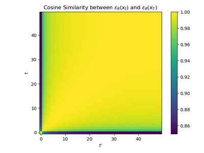
Figure 6: Plot of the cosine similarity between $\epsilon_{\theta}(x_{t},t)$ and $\epsilon_{\theta}(x_{t^{\prime}},t^{\prime})$ over $N=50$ steps of DDIM denoising on the CIFAR-10 dataset. Each cell is the average result of 1000 runs.

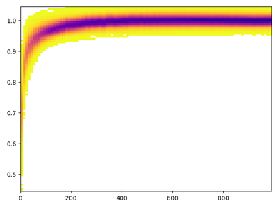
(a) Plot of $\left\lVert\epsilon_{\theta}(x_{t},\sigma_{t})\right\lVert/\sqrt{n}$ against $t$.

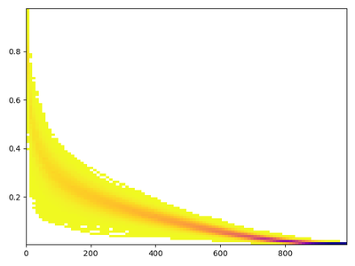
(b) Plot of $\left\lVert\epsilon_{\theta}(x_{0}+\sigma_{t}\epsilon,\sigma_{t})-\epsilon\right\lVert/\sqrt{n}$ against $t$.

Figure 7: Plots of the norm of the denoiser at different stages of denoising, as well as the ability of the denoiser to accurately predict the added noise as a function of noise added.

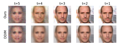
Figure 8: A comparison of our sampler with DDIM on the CelebA dataset with $N=5$ steps.

E.2 Distance Function Properties

We test 1 and 2 on pretrained networks. If 1 is true, then $\left\lVert\epsilon_{\theta}(x_{t},\sigma_{t})\right\lVert\sqrt{n}=\left\lVert\nabla{\rm dist}_{\mathcal{K}}(x_{t})\right\lVert=1$ for every $x_{t}$ along the DDIM trajectory. In Figure 7(a), we plot the distribution of norm of the denoiser $\epsilon_{\theta}(x_{t},\sigma_{t})$ over the course of many runs of the DDIM sampler on the CIFAR-10 model for $N=100$ steps ($t=1000,990,\ldots,20,10,0$). This plot shows that $\left\lVert\epsilon_{\theta}(x_{t},\sigma_{t})\right\lVert/\sqrt{n}$ stays approximately constant and is close to 1 until the end of the sampling process. We next test 3, which implies 2 by C.4. We do this by first sampling a fixed noise vector $\epsilon$, next adding different levels of noise $\sigma_{t}$, then using the denoiser to predict $\epsilon_{\theta}(x_{0}+\sigma_{t}\epsilon,\sigma_{t})$. In Figure 7(b), we plot the distribution of $\left\lVert\epsilon_{\theta}(x_{0}+\sigma_{t}\epsilon,\sigma_{t})-\epsilon\right\lVert/\sqrt{n}$ over different levels of $t$, as a measure of how well the denoiser predicts the added noise.

E.3 Choice of $\gamma$

We motivate our choice of $\gamma=2$ in Algorithm 2 with the following experiment. For varying $\gamma$, Figure 9 reports FID scores of our sampler on the CIFAR-10 and CelebA models for $N=5,10,20$ timesteps using the $\sigma_{t}$ schedule described in Section F.3. As shown, $\gamma\approx 2$ achieves the optimal FID score over different datasets and choices of $N$.

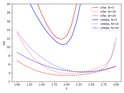
Figure 9: Plot of FID score against $\gamma$ for our second-order sampling algorithm on the CIFAR-10 and CelebA datasets for $N=5,10,20$ steps.

Appendix F Experiment Details

F.1 Pretrained Models

The CIFAR-10 model and architecture were based on that in [13], and the CelebA model and architecture were based on that in [40]. The specific checkpoints we use are provided by [22]. We also use Stable Diffusion 2.1 provided in https://huggingface.co/stabilityai/stable-diffusion-2-1. For the comparison experiments in Figure 4, we implemented our gradient estimation sampler to interface with the HuggingFace diffusers library and use the corresponding implementations of UniPC, DPM++, PNDM and DDIM samplers with default parameters.

F.2 FID Score Calculation

For the CIFAR-10 and CelebA experiments, we generate 50000 images using our sampler and calculate the FID score using the library in https://github.com/mseitzer/pytorch-fid. The statistics on the training dataset were obtained from the files provided by [22]. For the MS-COCO experiments, we generated images from 30k text captions drawn from the validation set, and computed FID with respect to the 30k corresponding images.

F.3 Our Selection of $\sigma_{t}$

Let $\sigma_{1}^{\text{DDIM}(N)}$ be the noise level at $t=1$ for the DDIM sampler with $N$ steps. For the CIFAR-10 and CelebA models, we choose $\sigma_{1}=\sqrt{\sigma_{1}^{\text{DDIM}(N)}}$ and $\sigma_{0}=0.01$. For CIFAR-10 $N=5,10,20,50$ and CelebA $N=5$ we choose $\sigma_{N}=40$ and for CelebA $N=10,20,50$ we choose $\sigma_{N}=80$. For Stable Diffusion, we use the same sigma schedule as that in DDIM.

F.4 Text Prompts

For the text to image generation in Figure 4, the text prompts used are:

• “A digital Illustration of the Babel tower, 4k, detailed, trending in artstation, fantasy vivid colors”

• “London luxurious interior living-room, light walls”

• “Cluttered house in the woods, anime, oil painting, high resolution, cottagecore, ghibli inspired, 4k”

References

- [1] Bao, F., Li, C., Zhu, J., and Zhang, B. Analytic-dpm: an analytic estimate of the optimal reverse variance in diffusion probabilistic models. arXiv preprint arXiv:2201.06503 (2022).
- [2] Bengio, Y., Courville, A., and Vincent, P. Representation learning: A review and new perspectives. IEEE transactions on pattern analysis and machine intelligence 35, 8 (2013), 1798–1828.
- [3] bin Waheed, U., Haghighat, E., Alkhalifah, T., Song, C., and Hao, Q. Pinneik: Eikonal solution using physics-informed neural networks. Computers & Geosciences 155 (2021), 104833.
- [4] Chan, S. H., Wang, X., and Elgendy, O. A. Plug-and-play admm for image restoration: Fixed-point convergence and applications. IEEE Transactions on Computational Imaging 3, 1 (2016), 84–98.
- [5] Chi, C., Feng, S., Du, Y., Xu, Z., Cousineau, E., Burchfiel, B., and Song, S. Diffusion policy: Visuomotor policy learning via action diffusion. arXiv preprint arXiv:2303.04137 (2023).
- [6] Chung, H., Sim, B., Ryu, D., and Ye, J. C. Improving diffusion models for inverse problems using manifold constraints. arXiv preprint arXiv:2206.00941 (2022).
- [7] De Bortoli, V. Convergence of denoising diffusion models under the manifold hypothesis. arXiv preprint arXiv:2208.05314 (2022).
- [8] Delfour, M. C., and Zolésio, J.-P. Shapes and geometries: metrics, analysis, differential calculus, and optimization. SIAM, 2011.
- [9] Dhariwal, P., and Nichol, A. Diffusion models beat GANs on image synthesis. Advances in Neural Information Processing Systems 34 (2021), 8780–8794.
- [10] Federer, H. Curvature measures. Transactions of the American Mathematical Society 93, 3 (1959), 418–491.
- [11] Fefferman, C., Mitter, S., and Narayanan, H. Testing the manifold hypothesis. Journal of the American Mathematical Society 29, 4 (2016), 983–1049.
- [12] Heusel, M., Ramsauer, H., Unterthiner, T., Nessler, B., and Hochreiter, S. Gans trained by a two time-scale update rule converge to a local nash equilibrium. Advances in neural information processing systems 30 (2017).
- [13] Ho, J., Jain, A., and Abbeel, P. Denoising diffusion probabilistic models. Advances in Neural Information Processing Systems 33 (2020), 6840–6851.
- [14] Kadkhodaie, Z., and Simoncelli, E. P. Solving linear inverse problems using the prior implicit in a denoiser. arXiv preprint arXiv:2007.13640 (2020).
- [15] Karras, T., Aittala, M., Aila, T., and Laine, S. Elucidating the design space of diffusion-based generative models. arXiv preprint arXiv:2206.00364 (2022).
- [16] Kawar, B., Elad, M., Ermon, S., and Song, J. Denoising diffusion restoration models. arXiv preprint arXiv:2201.11793 (2022).
- [17] Kong, Z., Ping, W., Huang, J., Zhao, K., and Catanzaro, B. Diffwave: A versatile diffusion model for audio synthesis. arXiv preprint arXiv:2009.09761 (2020).
- [18] Krizhevsky, A., Hinton, G., et al. Learning multiple layers of features from tiny images.
- [19] Le Pendu, M., and Guillemot, C. Preconditioned plug-and-play admm with locally adjustable denoiser for image restoration. SIAM Journal on Imaging Sciences 16, 1 (2023), 393–422.
- [20] Lichtenstein, M., Pai, G., and Kimmel, R. Deep eikonal solvers. In Scale Space and Variational Methods in Computer Vision: 7th International Conference, SSVM 2019, Hofgeismar, Germany, June 30–July 4, 2019, Proceedings 7 (2019), Springer, pp. 38–50.
- [21] Lin, T.-Y., Maire, M., Belongie, S., Hays, J., Perona, P., Ramanan, D., Dollár, P., and Zitnick, C. L. Microsoft coco: Common objects in context. In Computer Vision–ECCV 2014: 13th European Conference, Zurich, Switzerland, September 6-12, 2014, Proceedings, Part V 13 (2014), Springer, pp. 740–755.
- [22] Liu, L., Ren, Y., Lin, Z., and Zhao, Z. Pseudo numerical methods for diffusion models on manifolds. arXiv preprint arXiv:2202.09778 (2022).
- [23] Liu, R., Wu, R., Van Hoorick, B., Tokmakov, P., Zakharov, S., and Vondrick, C. Zero-1-to-3: Zero-shot one image to 3d object. arXiv preprint arXiv:2303.11328 (2023).
- [24] Liu, Z., Luo, P., Wang, X., and Tang, X. Deep learning face attributes in the wild. In Proceedings of International Conference on Computer Vision (ICCV) (December 2015).
- [25] Lu, C., Zhou, Y., Bao, F., Chen, J., Li, C., and Zhu, J. Dpm-solver: A fast ode solver for diffusion probabilistic model sampling in around 10 steps. arXiv preprint arXiv:2206.00927 (2022).
- [26] Lu, C., Zhou, Y., Bao, F., Chen, J., Li, C., and Zhu, J. Dpm-solver++: Fast solver for guided sampling of diffusion probabilistic models. arXiv preprint arXiv:2211.01095 (2022).
- [27] Meng, C., He, Y., Song, Y., Song, J., Wu, J., Zhu, J.-Y., and Ermon, S. Sdedit: Guided image synthesis and editing with stochastic differential equations. In International Conference on Learning Representations (2021).
- [28] Nichol, A. Q., and Dhariwal, P. Improved denoising diffusion probabilistic models. In International Conference on Machine Learning (2021), PMLR, pp. 8162–8171.
- [29] Park, J. J., Florence, P., Straub, J., Newcombe, R., and Lovegrove, S. Deepsdf: Learning continuous signed distance functions for shape representation. In Proceedings of the IEEE/CVF conference on computer vision and pattern recognition (2019), pp. 165–174.
- [30] Poole, B., Jain, A., Barron, J. T., and Mildenhall, B. Dreamfusion: Text-to-3d using 2d diffusion. arXiv preprint arXiv:2209.14988 (2022).
- [31] Pope, P., Zhu, C., Abdelkader, A., Goldblum, M., and Goldstein, T. The intrinsic dimension of images and its impact on learning. arXiv preprint arXiv:2104.08894 (2021).
- [32] Ramesh, A., Dhariwal, P., Nichol, A., Chu, C., and Chen, M. Hierarchical text-conditional image generation with clip latents. arXiv preprint arXiv:2204.06125 (2022).
- [33] Rick Chang, J., Li, C.-L., Poczos, B., Vijaya Kumar, B., and Sankaranarayanan, A. C. One network to solve them all–solving linear inverse problems using deep projection models. In Proceedings of the IEEE International Conference on Computer Vision (2017), pp. 5888–5897.
- [34] Rombach, R., Blattmann, A., Lorenz, D., Esser, P., and Ommer, B. High-resolution image synthesis with latent diffusion models. In Proceedings of the IEEE/CVF Conference on Computer Vision and Pattern Recognition (2022), pp. 10684–10695.
- [35] Saharia, C., Chan, W., Saxena, S., Li, L., Whang, J., Denton, E., Ghasemipour, S. K. S., Ayan, B. K., Mahdavi, S. S., Lopes, R. G., et al. Photorealistic text-to-image diffusion models with deep language understanding. arXiv preprint arXiv:2205.11487 (2022).
- [36] Scieur, D., Roulet, V., Bach, F., and d’Aspremont, A. Integration methods and optimization algorithms. Advances in Neural Information Processing Systems 30 (2017).
- [37] Sethian, J. A. A fast marching level set method for monotonically advancing fronts. Proceedings of the National Academy of Sciences 93, 4 (1996), 1591–1595.
- [38] Smith, J. D., Azizzadenesheli, K., and Ross, Z. E. Eikonet: Solving the eikonal equation with deep neural networks. IEEE Transactions on Geoscience and Remote Sensing 59, 12 (2020), 10685–10696.
- [39] Sohl-Dickstein, J., Weiss, E., Maheswaranathan, N., and Ganguli, S. Deep unsupervised learning using nonequilibrium thermodynamics. In International Conference on Machine Learning (2015), PMLR, pp. 2256–2265.
- [40] Song, J., Meng, C., and Ermon, S. Denoising diffusion implicit models. arXiv preprint arXiv:2010.02502 (2020).
- [41] Song, Y., Dhariwal, P., Chen, M., and Sutskever, I. Consistency models. arXiv preprint arXiv:2303.01469 (2023).
- [42] Song, Y., and Ermon, S. Generative modeling by estimating gradients of the data distribution. Advances in neural information processing systems 32 (2019).
- [43] Song, Y., Sohl-Dickstein, J., Kingma, D. P., Kumar, A., Ermon, S., and Poole, B. Score-based generative modeling through stochastic differential equations. arXiv preprint arXiv:2011.13456 (2020).
- [44] Tevet, G., Raab, S., Gordon, B., Shafir, Y., Cohen-Or, D., and Bermano, A. H. Human motion diffusion model. arXiv preprint arXiv:2209.14916 (2022).
- [45] Vershynin, R. High-dimensional probability: An introduction with applications in data science, vol. 47. Cambridge university press, 2018.
- [46] Vincent, P. A connection between score matching and denoising autoencoders. Neural computation 23, 7 (2011), 1661–1674.
- [47] Welling, M., and Teh, Y. W. Bayesian learning via stochastic gradient langevin dynamics. In Proceedings of the 28th international conference on machine learning (ICML-11) (2011), Citeseer, pp. 681–688.
- [48] Zhang, Q., and Chen, Y. Fast sampling of diffusion models with exponential integrator. arXiv preprint arXiv:2204.13902 (2022).
- [49] Zhao, W., Bai, L., Rao, Y., Zhou, J., and Lu, J. Unipc: A unified predictor-corrector framework for fast sampling of diffusion models. arXiv preprint arXiv:2302.04867 (2023).