Learned Spatial Data Partitioning

Abstract.

Due to the significant increase in the size of spatial data, it is essential to use distributed parallel processing systems to efficiently analyze spatial data. In this paper, we first study learned spatial data partitioning, which effectively assigns groups of big spatial data to computers based on locations of data by using machine learning techniques. We formalize spatial data partitioning in the context of reinforcement learning and develop a novel deep reinforcement learning algorithm. Our learning algorithm leverages features of spatial data partitioning and prunes ineffective learning processes to find optimal partitions efficiently. Our experimental study, which uses Apache Sedona and real-world spatial data, demonstrates that our method efficiently finds partitions for accelerating distance join queries and reduces the workload run time by up to 59.4%.

1. Introduction

A large amount of spatial data, such as temperature data, traffic logs, and geo-tagged blog posts, is drastically increasing. We often analyze spatial data in many applications such as traffic control (Wei et al., 2018), human mobility analysis (Pang et al., 2020), disaster surveillance (Julian and Kochenderfer, 2019), mobility service (Pan et al., 2019), and route and point-of-interest recommendation (Liu et al., 2019; Sasaki et al., 2018). For efficient analysis of spatial data, it is essential to use distributed parallel processing systems for spatial data such as Sedona (Apache Sedona, 2021), SpatialHadoop (Eldawy and Mokbel, 2015), and others (Sevim et al., 2021; Aji et al., 2013; Xie et al., 2016; Tang et al., 2016; Sasaki, 2021).

Motivation. One of the fundamental functions of such systems is spatial data partitioning, which divides the whole area into sub-area (called partitions) and assigns data in the same partitions to computers for efficient parallel-processing (Eldawy et al., 2015). Existing spatial data partitioning methods focus only on data distributions to balance the computation costs among computers. However, it is difficult to obtain partitions that are optimized for data distributions, user queries, and computation frameworks.

Deep reinforcement learning (DRL for short) approach is effective for system optimization, including data partitioning (Hilprecht et al., 2020). To our knowledge, there are no studies on DRL-based spatial data partitioning. Since spatial data partitioning directly affects the performance of data processing, it is worth studying DRL-based spatial data partitioning to accelerate the processing of big spatial data.

Contribution. We study spatial data partitioning with deep reinforcement learning. We have three main contributions; problem formulation, algorithm, and experiment.

First, we formalize a spatial data partitioning problem in the context of reinforcement learning. The characteristics of our problem are to consider not only distributions of spatial data but also the computation environment (e.g., a computing system) and workloads (e.g., the set of queries). This problem formulation aims at pursuing effective spatial data partitioning for each user.

Second, to address our spatial data partitioning problem, we develop a novel learning algorithm that efficiently explores actions for finding optimal partitions. Our algorithm has a $2$-phase learning strategy consisting of pre-training and main-training (Hester et al., 2018). In the pre-training phase, our algorithm trains a model by using pre-collected transitions (i.e., training data) based on existing spatial partitioning algorithms to avoid selecting less-effective actions during the main-training. In the main-training phase, it searches for optimal partitions and trains the model using transitions (i.e., sequences of actions). Our framework is extended to (1) improve the effectiveness by using preparing demos of partitioning-related transitions and (2) accelerate learning by reducing action space and pruning run time measurements based on the characteristics of spatial data processing.

Finally, we evaluate our method using Apache Sedona, the state-of-the-art distributed parallel processing system for big spatial data, with real-world datasets. We validate that the DRL-based approach is highly effective in accelerating big spatial data processing.

Reproducibility. We open our source codes, datasets, and workloads that we used in an experimental study at Github https://github. com/OnizukaLab/Spatial-Data-Partitioning-using-DRL.

2. Preliminaries

We explain spatial data partitioning and deep reinforcement learning as preliminaries.

2.1. Spatial data partitioning

Spatial data partitioning is a function that determines how the area divides into partitions. We define spatial data partitioning as follows:

Definition 2.1.

Given a spatial dataset $\mathcal{D}$, spatial data partitioning is a task to divide the whole area in $\mathcal{D}$ into partitions and then assign sets of data in the same partitions to computers. We denote the set of partitions by $\mathcal{P}$. $\mathcal{P}$ needs to satisfy that any partitions $P\in\mathcal{P}$ are distinct and it covers the whole area in $\mathcal{D}$.

Distributed parallel processing systems compose of multiple computers. The sets of data in partitions are assigned to computers and each computer parallelly processes its assigned data. If computers need to access data that are held by other computers, they transfer their data (which is called shuffle), and finally, the processing results are aggregated to answer users.

Spatial data partitioning has two main objectives. First, since a set of data that are spatially close to each other is often accessed together, the partitions should reduce the communication costs between computers. Second, since computers parallelly process their data, partitions should have an equal amount of data to balance the burden of data processing. These requirements are essential to scale out to multiple computers.

2.2. Deep reinforcement learning

Reinforcement learning (Kaelbling et al., 1996) is a process in which an agent repeatedly interacts with a Markov decision process to autonomously acquire information that serves as a supervisory signal while deriving optimal strategies. The agent selects action $a_{i}$ on state $s_{i}$ by policy $\pi(s_{i},a_{i})$, and then observes reward $r(s_{i},a_{i})$ and obtains the next state $s_{i+1}$ caused by $a_{i}$. It repeats this process by selecting $a_{1}$ on $s_{0}$ until the state $s_{n}$ satisfies given conditions. We define $\mathcal{A}$ and $\mathcal{S}$ as the action and state spaces, respectively. A block of processes from $a_{1}$ to $a_{n}$ is called episode, and a four-pair $(s_{t},a_{t},r_{t},s_{t+1})$ in an episode at step $t$ is called transition.

The goal of reinforcement learning is to maximize the cumulative reward $\Sigma_{k=0}^{n}r(s_{t+k},a_{t+k})$ at state $s_{t}$. It considers the action-value function $Q_{\pi}(s,a)=E[\Sigma_{k=0}^{\infty}\gamma^{k}r_{t+k}|s_{t}=s,a_{t}=a]$, which is the expected cumulative reward when the agent follows policy $\pi$. If we find the optimal function $Q^{*}$ to maximize the expected cumulative reward, we can derive the optimal policy as $\pi^{*}(s)=$ arg max${}_{a\in\mathcal{A}}Q^{*}(s,a)$ for $\forall s\in\mathcal{S}$.

Deep reinforcement learning aims at approximating the action-value function by using deep neural networks. It is often difficult to maintain the function for any pairs of actions and states if their patterns are tremendous. When we train the deep neural network models with tremendous patterns, the agent can select an optimal action on each state following these models.

Q-learning and Deep Q-network. Q-learning (Watkins and Dayan, 2004), a typical reinforcement learning method, selects a high-value action in terms of the action-value function $Q$. By repeatedly observing the state and reward, the optimal action-value function is updated using the temporal difference error between the outputs of $Q$, which are called $Q$-values, in the next and current states.

(1) $$\begin{split}Q(s_{t},a_{t}){\leftarrow}&Q(s_{t},a_{t})+\\ &\!\!\!\!\!\!\alpha\{r_{t+1}+\gamma\max_{a\in\mathcal{A}}Q(s_{t+1},a_{t+1})-Q(s_{t},a_{t})\}\end{split}$$

If the action and/or state spaces are large or continuous, the number of combinations becomes very large, making it difficult to maintain $Q$-values in the table.

Deep Q-Network (DQN), which is an extension of Q-learning, approximates the function $Q$ and the policy function in Q-network. Similar to Q-learning, DQN aims to make $Q(s_{t},a_{t})$ close to $r_{t}+\gamma\max Q(s_{t+1},a_{t+1})$, so the Q-network is trained using the error function $L$ and the current $Q$-value as follows:

(2) $$L=\sum_{(s_{t},a_{t},r_{t},s_{t+1})\in B}(r_{t}+\gamma\max Q(s_{t+1},a_{t+1};\theta)-Q(s_{t},a_{t};\theta))^{2},$$

where $\theta$ and $B$ are a deep neural network model and a set of past transitions, respectively.

3. Related work

We review existing works related to spatial data partitioning and system optimization with deep learning. To the best of our knowledge, there are no deep learning-based methods for computing spatial data partitioning.

Spatial data partitioning We review some typical algorithms for spatial data partitioning. Uniform grid is the simplest method that divides the area into equal-sized partitions. Quad-tree (Finkel and Bentley, 1974) and KDB-tree (Robinson, 1981) are methods that repeatedly divide the partition that includes the largest number of data (initially starts a single partition covering the whole area). Quad-tree divides the partition into equal-sized four partitions, while KDB-tree divides the partition into two partitions so that the two partitions have the same amount of data. Vu (Vu et al., 2021b) proposes a method for incremental updates of spatial partitions which utilize estimation of query execution time. Vu et al. (Vu et al., 2020) proposed a method that selects optimal spatial partitioning methods (e.g., KDB-tree and Quad-tree) by using DRL. This method just selects methods among the given ones, instead that it does not aim at computing partitions. Aly et al. (Aly et al., 2015) proposed a spatial partitioning method that uses a given set of range and kNN queries. This aims to reduce the communication between computers, but it can use only range and kNN queries instead of spatial join, so it is not applicable to general settings that include many query types.

Hilprecht et al. (Hilprecht et al., 2020) proposed a DRL-based hash partitioning, but it does not focus on spatial partitioning. It is well known that hash partitioning is not effective for spatial queries.

System optimization with deep learning. Spatial data partitioning is one of the tasks in system optimization, so we review system optimization techniques using deep learning (Li, 2017). Spatial partitioning is similar to indexing techniques on spatial/multi-dimensional data, and many learning indexing techniques are developed, such as Flood (Nathan et al., 2020), Tsunami (Ding et al., 2020), LISA (Li et al., 2020), Qd-tree (Yang et al., 2020), RLR-tree (Gu et al., 2021), and RSMI (Qi et al., 2020). They build data blocks (i.e., the set of data) and construct index structures to accelerate spatial query processing on a single machine. Since they do not assume spatial partitioning, their blocks are either unsophisticated or inapplicable for spatial partitioning, for example, Flood divides data into blocks based on the data distribution on a single axis and the blocks of Qd-tree are not distinct. Lan et al. (Lan et al., 2020) proposed a DRL-based index recommendation. Vu et al.(Vu et al., 2021a) develop a query optimizer for spatial join based on neural networks, which aims to estimate the cardinality and select join algorithms. These works do not aim to divide the dataset into data blocks

4. Problem Formulation

We formulate spatial data partitioning as a new reinforcement learning problem. First, we define our problem as follows:

Problem: Given a spatial dataset $\mathcal{D}$, a workload $W$ (i.e., the set of queries and their frequencies), and a computation environment (i.e., system and the number of computers), the goal is to find the set of partitions $\mathcal{P}$ that minimizes the run time of the workload for $\mathcal{D}$ on the computation environment.

In the following, we define the initial setup, state, action, and reward for this problem, respectively.

Initial setup. We form a map that covers the locations of the given data in a two-dimensional space as an environment for a DRL agent. We divide this map into a set of uniform grid cells. The agent constructs partitions by adding new boundaries on each grid line.

State: The state is obtained from the current partitions and data distribution. We define that state $s$ is a set of status $s_{(i,j)}$ for each grid cell $(i,j)$ as follows:

(3) $$s_{(i,j)}=(h_{\mathit{(i,j)}},v_{\mathit{(i,j)}},p_{\mathit{(i,j)}}),$$

where $i$ and $j$ specify the upper-left coordinate of the grid cell. $h\in\{0,1\}$ and $v\in\{0,1\}$ denote the absence/presence of horizontal and vertical boundaries on the top and left sides of the cell, respectively. $p_{\mathit{(i,j)}}$ denotes the ratio of the numbers of data in the cell and partition. We define $p_{\mathit{(i,j)}}=\frac{|\mathcal{D}_{\mathit{(i,j)}}|\cdot|P_{\mathit{(i,j)}}|}{|\mathcal{D}|^{2}}$, where $|\mathcal{D}|$, $|\mathcal{D}_{\mathit{(i,j)}}|$, and $|P_{\mathit{(i,j)}}|$ are the numbers of data in the given dataset $\mathcal{D}$, in a cell $(i,j)$, and in a partition that covers $(i,j)$, respectively.

Action. The action $a\in\mathcal{A}$ is an operation to add a new boundary line. We define the action as follows:

(4) $$a=(i,j,\mathit{dir}),$$

where $i$ and $j$ are the coordinates of the starting point of the action and $\mathit{dir}\in\{\mathit{right},\mathit{down}\}$ specifies the direction of the boundary from $(i,j)$, i.e., rightward or downward. To avoid invalid actions, the starting points need to be satisfied either of conditions; (1) $\mathit{dir}=\mathit{right}$, $h(i,j)=0$, and $v(i,j)=1$ or (2) $\mathit{dir}=\mathit{down}$, $h(i,j)=1$, and $v(i,j)=0$.

Reward. The reward $r$ is computed based on the run time $C(\mathcal{P},w)$ for an operator $w$ on a set of partition $\mathcal{P}$ to the spatial dataset in the computation environment. It enables to maximizing the reward $r$ to optimize execution in the given computing environment. The reward $r$ is evaluated as follows:

(5) $$r=\left(\sum_{w_{i}\in W}{f_{i}}\cdot\frac{C(\mathcal{P}_{\mathit{b}},w_{i})}{C(\mathcal{P}_{\mathit{e}},w_{i})}\right)^{2},$$

where $w_{i}$, $f_{i}$, $\mathcal{P}_{\mathit{e}}$, and $\mathcal{P}_{b}$ indicate a query in the workload, a frequency of operator $w_{i}$, a set of partitions at the end of the episode, and the best set of partitions we found during training, respectively. This equation evaluates a relative to the best run time up to that on the partitions at the current episode. The value is squared to emphasize the difference between the run time on $\mathcal{P}_{b}$ and $\mathcal{P}_{e}$. If $r>1$, $\mathcal{P}_{e}$ is better than $\mathcal{P}_{b}$. Note that computing all queries in the workload is costly compared with other procedures such as training deep neural networks.

Example. Figure 1 illustrates an example of states and actions for obtaining three partitions. Initially, there are no boundaries (i.e., a single partition). In this example, the agent takes $a_{1}=(0,3,down)$ and $a_{2}=(2,3,right)$. The status of cell $s_{(2,3)}$ changes by adding boundary lines. $p_{(2,3)}$ becomes smaller because the percentage of the number of data in the partition becomes smaller instead of that in the cell is constant. We run the workload and obtain the reward for the episode after computing three partitions.

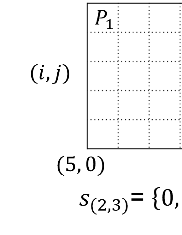
Figure 1. Example of actions and states: the agent selects actions $a_{t}$ to add new boundaries depending on the state $s_{t}$.

5. Learning Algorithm

This section proposes a learning algorithm for our problem formulated in Section 4. We have two challenges to solve our problem. First, the action and state spaces are very large to find optimal partitions. Common DRL algorithms start the random selection of actions. We should efficiently explore actions by capturing the characteristics of spatial data partitioning. Second, our problem takes a large training time because of measuring the run time of workload at the end of each episode to compute rewards. For efficient training, we should reduce the run time while keeping the effectiveness of training.

To address the above challenges, we design a learning strategy consisting of (1) pre-training using demo data which is a set of pre-collected transitions and (2) main-training. Our learning framework trains our model by effectively combining DQN with imitation learning based on our strategy. Sections 5.1 and 5.2 present our learning strategy and learning framework, respectively. Section 5.3 presents our algorithm.

5.1. Learning strategy

Our algorithm is based on the following ideas:

• Pre-training by effective demo data: Our algorithm builds a model that follows existing algorithms for spatial data partitioning. This model avoids selecting less-effective actions at early episodes of the main-training phase.

• Effective new action choice: We add a new action that makes a boundary close to the best partitions. It supports exploring effective actions.

• Pruning run time measurement: Our algorithm prunes ineffective executions of the workload to reduce the training time.

These ideas are specialized for our problem formulation, and thus all of them are not applied to the DRL approach yet. We explain pre-training and main-training phases.

Pre-training. In the pre-training phase, we train our model using only demo data so that the agent similarly selects actions in demo data. We first collect transitions from actions based on existing partitioning algorithms and then use the transitions as demo data. It makes the initial values of the agent’s actions appropriate for the distribution of a given dataset before the main-training. Therefore, this pre-training phase drastically reduces random actions in the early episodes of the learning processes, which is essentially an exhaustive trial-and-error process.

The selection of demo data may not obtain exactly the same partition computed from existing methods because the boundaries of our partitions are limited on pre-defined grid cells. We select the closest boundaries to those of existing methods. Our strategy guarantees that the run time on the best partitions obtained by our algorithm is at least the (almost) best performance among existing methods by choosing the most effective method for generating demo data.

Main-training. In the main-training phase, we search for actions that construct a set of partitions better than those generated by the pre-collected demo data. The basic procedures of the main-training phase are that the agent repeatedly selects its actions probabilistically by using an $\epsilon$-greedy method (Thrun and Littman, 2000), and then when the number of partitions reaches the number of machines, it distributes data into computers according to the partitions, executes the workload, and computes a reward. Our algorithm repeatedly runs these procedures until reaching the given number of episodes.

Our algorithm adds new action choices to the $\epsilon$-greedy method. In the common $\epsilon$-greedy method, the agent selects the best action approximated by a model or a random action. We add actions of one grid-shift from the best action to the $\epsilon$-greedy method. In spatial data partitioning, better partitions than the current best ones are often to be found near the current best partitions, and thus such one grid-shift actions help to search for the optimal partitions effectively. We can find effective partitions efficiently by intensively exploring actions near the approximated best action.

We reduce the training time by terminating the workload execution for partitions that are clearly less-effective. Specifically, the workload execution stops whenever the execution time of one of the queries in the workload exceeds a certain level compared with that on $\mathcal{P}_{b}$. In this case, its reward $r$ is set to a predefined small value.

5.2. Learning framework

Our learning framework consists of an agent, a learner of the network that approximates the action values of the agent, and two replay memories. These replay memories are called demo and agent memories, storing the demo data and other transitions, respectively. The demo memory is used for imitation learning. We note that it uses only demo memory to train deep neural networks in the pre-training phase.

In the main-training phase, our framework adds transitions that construct better partitions than $\mathcal{P}_{b}$ to demo data. This contributes to exploring better actions by imitating the current best actions instead of the pre-collected actions. More concretely, if $r>1$, it adds the transitions to the demo data. In addition, we add transitions with $r\leq 1$ to another memory because such data is effective to learn the wide variety of action values.

We use two Q-networks, main network $\theta$ and target network $\theta^{\prime}$, following existing works (Mnih et al., 2015; Nair et al., 2015). The target network is used for stable learning. The learner trains the main network and periodically overwrites $\theta^{\prime}$ by $\theta$. It also updates priorities for transitions in memories using prioritized experience replay (Schaul et al., 2016), which is effective to sample data for training the Q-network. The input and output dimensions of the Q-network are the size of the state and action spaces, respectively. Mini-batch data sampled from both memories according to the priorities and the ratio $\rho$ that controls the importance of memories. The imitation learning guarantees that the mini-batch data include effective transitions sampled from the demo memory, resulting in Q-networks that are trained to find better partitions.

For the loss function, we use three losses. First, loss $L_{N}(\theta)$ is the temporal difference error considering the rewards of $n$ steps ahead using multi-step learning (Asis et al., 2018) as follows:

(6) $$\begin{split}L_{N}(\theta)=\sum_{(s_{i},a_{i},r_{i},s_{i+n})\in B}(r_{i}+\gamma^{1}r_{i+1}+...+\gamma^{n+1}r_{i+n-1}\\ +arg~{}max_{a\in\mathcal{A}}Q_{\theta^{\prime}}(s_{i+n},a_{i+n})-Q_{\theta}(s_{i},a_{i}))^{2}\end{split}$$

This loss accelerates the propagation of the reward, which is obtained only at the end of the episode, thereby improving learning efficiency.

Second, to imitate the actions in demo data, we use large margin classification loss $L_{C}(\theta)$ (Hester et al., 2018), which is applied only to the demo data. $L_{C}(\theta)$ is computed as follows:

(7) $$L_{C}(\theta)=\max_{a\in\mathcal{A}}[Q(s,a)+l(a_{C},a)]-Q(s,a_{C}),$$

where $a_{C}$ and $l(a_{C},a)$ are an action in demo data and a function that outputs $0$ when $a=a_{C}$ and positive otherwise, respectively. $L_{C}(\theta)$ becomes zero if $a_{C}$ is selected as the best action, otherwise the loss becomes larger to imitate the demo data. This loss effectively accelerates imitations.

Finally, we use the L2 regularization loss, $L_{l2}(\theta)$, for parameters $\gamma_{i}$ of main-network $\theta$ to suppress overfitting to a small number of demo data.

(8) $$L_{l2}(\theta)=\sum_{\gamma_{i}\in\theta}{|\gamma_{i}|}^{2}$$

We apply the three losses to loss $L(\theta)$ as follows:

(9) $$L(\theta)=\lambda_{1}L_{N}(\theta)+\lambda_{2}L_{C}(\theta)+\lambda_{3}L_{l2}(\theta),$$

where $\lambda_{1}$, $\lambda_{2}$, and $\lambda_{3}$ are the weights for the corresponding losses.

input : Dataset $\mathcal{D}$, workload $W$, the number of computers $M$, demo data $B_{\mathit{d}}$, demo partitions $\mathcal{P}_{d}$

parameter : Update weight frequency $U$, demo ratio $\rho$, the number of episodes $e_{max}$

output : Best partitions $\mathcal{P}_{b}$

1 procedure Pre-training

2 Initialize the main network $\theta$ and target network $\theta^{\prime}$

3 $B_{\mathit{demo}}\leftarrow B_{\mathit{d}}$

4

5for $e=1,\ldots,e_{max}$ do

6       Sample mini-batch $B$ from $B_{\mathit{demo}}$

7       Train main network $\theta$ with $B$

8       if $(e\bmod U)=0$ then $\theta^{\prime}\leftarrow\theta$

9       Generate partitions $\mathcal{P}_{e}$ by agent actions

10       if $\mathcal{P}_{e}=\mathcal{P}_{d}$ then break

11

12procedure Main-training

13 $\mathit{step}\leftarrow 0$, $\mathcal{P}_{b}\leftarrow\mathcal{P}_{d}$, $B_{\mathit{agent}}\leftarrow\varnothing$

14 for $e=1,\ldots,e_{max}$ do

15       Reset state $s_{0}$, $B_{\mathit{tmp}}\leftarrow\varnothing$

16       for $t=1,\ldots,M-1$ do

17             Choose action $a_{t}$ with our $\epsilon$-greedy method by $\theta$

18             Execute action $a_{t}$ and observe state $s_{t}$

19             if $t\neq M-1$ then

20                   $B_{\mathit{tmp}}\leftarrow B_{\mathit{tmp}}\cup\{(s_{t},a_{t},0,s_{t+n})\}$

21                  

22            else

23                   Distribute partitions $\mathcal{P}_{e}$ to computers

24                   Run operators in $W$

25                   $r_{t}=(\sum_{w_{i}\in W}{f_{i}}\cdot\frac{C(\mathcal{P}_{b},w_{i})}{C(\mathcal{P}_{e},w_{i})})^{2}$

26                   $B_{\mathit{tmp}}\leftarrow B_{\mathit{tmp}}\cup\{(s_{t},a_{t},r_{t},s_{t+n})\}$

27                   if $r>1$ then

28                         $B_{\mathit{demo}}\leftarrow B_{\mathit{demo}}\cup B_{\mathit{tmp}}$

29                         $\mathcal{P}_{b}\leftarrow\mathcal{P}_{e}$

30                        

31                  else

32                         $B_{\mathit{agent}}\leftarrow B_{\mathit{agent}}\cup B_{\mathit{tmp}}$

33                  

34            Sample mini-batch $B$ from $B_{\mathit{demo}}$ and $B_{\mathit{agent}}$

35             Train main network $\theta$ with $B$

36             $\mathit{step}\leftarrow\mathit{step}+1$

37             if $(\mathit{step}\bmod U)=0$ then $\theta^{\prime}\leftarrow\theta$

38      

Algorithm 1 Learning algorithm

5.3. Algorithm

Algorithm 1 shows a pseudo-code of our learning algorithm. In the pre-training phase, we store the pre-collected demo data to the demo memory $B_{\mathit{demo}}$ (line 3) and then train the main network $\theta$ using the mini-batch data sampled from demo data (lines 4–9). We repeat the training until the partition $\mathcal{P}_{e}$ constructed by the agent is the same as the partitions $\mathcal{P}_{d}$ that demo data constructs.

In the main-training phase, the agent repeatedly collects transitions. We set the reward $r_{t}$ for each step $t$ in the episode to zero (line 18) and measure the run time of the workload when the number of steps reaches $M-1$ (i.e., the numbers of partitions and computers are the same) to compute the reward (lines 20–22). All transitions during the episode are stored in a temporary memory $B_{\mathit{tmp}}$ (line 23) and allocated to the demo memory $B_{\mathit{demo}}$ or agent memory $B_{\mathit{agent}}$ according to the reward $r_{M-1}$ (lines 24–28). We use mini-batch data sampled at a rate $\rho$ specified from $B_{\mathit{demo}}$ and $B_{\mathit{agent}}$ to train $\theta$ (lines 29–30). $\theta$ overwrites the target network $\theta^{\prime}$ follows update frequency $U$ (line 32). Our algorithm outputs the best partitions $\mathcal{P}_{b}$ found during training after finishing $e_{max}$ episodes.

6. Experimental study

We designed the experiments to clarify the following questions: (1) Is our method effective compared with existing methods? (2) Does our method find partitions efficiently?

6.1. Experimental setting

Computation environment. We used Apache Sedona, the state-of-the-art distributed and parallel processing system for big spatial data (Apache Sedona, 2021). We used nine computers with a Linux server with 32GB of memory and an Intel Celeron G4930T CPU@3.00GHz processor. One computer was a master server and the others were workers (i.e., eight computers processed a given workload). Sedona provides spatial queries, such as kNN, range, and distance join, and partition methods, such as KDB-tree and R-tree. We evaluated two cases with and without a local index, which supports efficient data access from the workers to their own local data.

To design our setting, we consider the limitations of Sedona; (a) range and kNN queries use hash partitioning instead of spatial partitioning, (b) R-tree partitioning cannot control the number of partitions, and (c) Polygon data is not handled on spatial join. The design of our experimental study is following to these limitations.

Datasets. We used point-of-interest data in two different areas, the United States (US) and South America (SA), extracted from OpenStreetMap, and Integrated Marine Information System (Imis), which is. For each dataset, we randomly sampled 100,000 point-of-interest from the original datasets. Figure 2 shows data distributions. They have different area sizes and distributions.

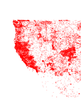
(a) OSM-US

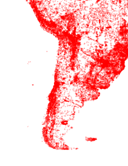
(b) OSM-SA

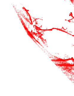
(c) Imis

Figure 2. Data distributions

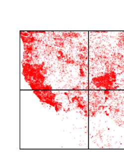
(a) Uniform grid

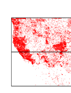
(b) Quad-tree

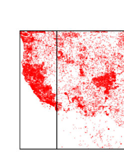
(c) KDB-tree

(d) Demo

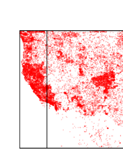
(e) Ours

Figure 3. Comparison of partitions in OSM-US

Workload. Our workload was a set of distance joins, each of which finds all pairs of data within a given distance threshold. Our workload included three distance thresholds, 500, 1000, and 5000 [meter] for US and SA, and 50, 100, and 500 [meters] for Imis, and we assumed two types of their frequencies; small skew and large skew. The small skew has 25, 50, and 25 [%] for the corresponding thresholds, respectively, while the large skew has 2, 3, and 95 [%].

Competitor. We used three spatial data partitioning methods; uniform grid, Quad-tree, and KDB-tree, which are originally implemented in Sedona.

Hyper-parameter tuning. We divided the entire map into $30\times 30$ grid cells. In our $\epsilon$-greedy method, the selection probabilities of random and grid shift actions were $\epsilon_{r}=0.1$ and $\epsilon_{s}=0.2$, respectively. We set the agent memory size to 10,000 and the demo memory size to 100. The mini-batch size for training was 32, and the percentage $\rho$ of demo data was $0.25$. Furthermore, we set the number of steps for multi-step learning to 3 and the reward discount rate to $\gamma=0.99$.

The Q-network consists of two hidden layers that have 1200 and 600 nodes, respectively, from the input side. The input and output dimensions depend on the grid size. In the case of our experimental setting, the input and output dimensions were 2833 (i.e., $31\times 31\times 3$) and 1800 (i.e., $30\times 30\times 2$), respectively. As parameters during training, the learning rate $\eta$ was 0.001, and we used Adam as the optimizer. The weights for the loss function were $\lambda_{1}=1.0$, $\lambda_{2}=1.0$, and $\lambda_{3}=10^{-5}$ according to the settings in the literature (Hester et al., 2018).

In the pruning execution of operators, when the run time of an operator was two times larger than that of $P_{b}$, we stopped running the workload and its reward was $0.2$. We ran each operator in the given workload three times to mitigate the fluctuation of run time, and the median of these measurements was used for computing rewards.

Table 1. Workload run time [sec]: The average run time of distance joins with each distance weighted by their frequencies. Bold and underline indicate the best and second best, respectively.

Data	idx	skew	Uniform	Quad	KDB	Demo	Ours
US	w/o	small	11.22	8.931	4.67	4.90	4.56
		large	15.83	13.29	8.65	8.95	6.71
	w/	small	3.35	3.82	3.00	3.00	1.78
		large	7.93	7.68	7.32	7.08	3.58
SA	w/o	small	11.72	11.91	6.92	7.22	6.90
		large	17.82	18.21	13.21	13.37	13.60
	w/	small	4.66	5.21	4.86	5.09	3.52
		large	11.29	11.12	11.19	11.97	8.34
Imis	w/o	small	16.74	12.69	8.77	8.93	9.49
		large	22.24	19.81	17.43	17.49	15.57
	w/	small	4.75	5.03	7.11	7.12	3.60
		large	11.18	11.84	16.21	15.87	7.84

6.2. Experimental result

6.2.1. Example of partitions

Figures 3 show the set of partitions constructed by each method on OSM-US. Uniform grid and Quad-tree have a large bias in the number of data in each partition because they ignore the number of data. On the other hand, KDB-tree has a small bias, because it always divides the area so that each partition has (almost) the same number of data. Demo was computed by KDB-tree, but there is a slight difference in the partitions because the boundaries are selected from the grid lines. Ours is slightly different from Demo to achieve a better workload run time. From this result, we can see that our algorithm imitates demo data and explores actions close to them. These examples show that our method can find effective partitions based on demo data.

6.2.2. Effectiveness

We evaluate the effectiveness of our method by the workload run time. Table 1 shows the run time needed for running the workload. We evaluated three cases: small skew without local index, large skew without local index, and small skew with local index.

Our method achieves the best performance among all the methods in all cases. This indicates that our method can adaptively divide datasets into partitions according to workloads and computational environments. When workloads have large skews, the difference between run times of ours and other methods becomes large, because our method optimizes partitions for workloads. Our method reduced the workload run time up to 59.4% compared with the second-best method.

Compared to the difference between run times without and with local index, run times with local index are smaller than those without local index in all methods. Our method achieves the smallest run time in both datasets, while KDB tree does not work well as uniform grid works in SA. In US, our method reduces the run time by 41 % compared to the second-best. The reason why the local index largely benefits our method is that our method uses computational environments (i.e., including local index) to optimize partitions, while other methods do not. This result shows that spatial partitioning should be taken not only in data distribution but also in computational environments such as local index. We validate that DRL-based spatial data partitioning improves the performance of workloads and computational environments.

(a) Search efficiency

Methods Learning time [hour] No optimization 120 (Done 924 episodes) w/o pre-training 98.4 w/o grid-shift action 72.5 w/o execution stop 120 (Done 2107 episodes) All optimization 65.5 (a) Learning time

Figure 4. Ablation study on the US dataset. We stopped training if a method did not finish 5,000 episodes within 120 hours.

6.2.3. Efficiency

We evaluated the learning time and learning efficiency of our method. For verifying the contribution of our learning strategy in Section 5.1 to the learning performance, we conducted an ablation study using the following five patterns: no optimization, w/o pre-training, w/o grid-shift action, w/o execution stop, and all optimization.

Figure 4 shows the search efficiency and the learning time. The search efficiency indicates the relationship between the number of episodes (x-axis) and the best run time during the training (y-axis); the shorter the run time during a small number of episodes, the more efficiently our method finds effective partitions.

All optimization significantly outperforms no optimizations in both learning time and search efficiency. This result indicates that our learning strategy is effective. In w/o pre-training, the initial performance depends on random partitions, so it takes many episodes to find effective partitions. We can confirm that the pre-training largely affects search efficiency. In w/o grid-shift action, the search efficiency is similar to all optimization. However, it often constructs less-effective partitions due to random actions, though the searches by random action have the potential to find better actions. This causes increasing the training time because less-effective partitions often take a large run time. In w/o execution stop, the learning time significantly increases. By comparing all optimization with w/o execution stop, we can confirm that our method sufficiently trains our models without computing strict rewards.

These results show that our learning strategy significantly contributes to efficient learning in our problem formulation.

7. Conclusion and Open Challenges

We studied deep reinforcement learning for spatial partitioning. We first formalized the spatial partitioning problem as deep reinforcement learning, and we developed a learning algorithm for the problem. Our algorithm combines Deep Q-network with imitation learning to explore actions effectively and efficiently. It includes three optimization techniques: pre-training by effective demo data partitioning, effective new action choice, and pruning run time measurement. Through our experiment using Apache Sedona and two real datasets, we validated that (i) our method is effective and accelerates spatial join processing and (ii) our optimization techniques reduce its learning time.

There are many open challenges to extending our work because we first studied learned spatial data partitioning. Promising challenges are to reduce learning time, select the optimal number of partitions instead of using the number of computers, and develop further optimal learning frameworks. Furthermore, it is interesting to investigate the performance of other distributed parallel processing systems and spatial queries.

References

- (1)
- Aji et al. (2013) Ablimit Aji, Fusheng Wang, Hoang Vo, Rubao Lee, Qiaoling Liu, Xiaodong Zhang, and Joel Saltz. 2013. Hadoop-GIS: a high performance spatial data warehousing system over mapreduce. PVLDB 6, 11 (2013), 1009–1020.
- Aly et al. (2015) Ahmed M Aly, Ahmed R Mahmood, Mohamed S Hassan, Walid G Aref, Mourad Ouzzani, Hazem Elmeleegy, and Thamir Qadah. 2015. Aqwa: adaptive query workload aware partitioning of big spatial data. PVLDB 8, 13 (2015), 2062–2073.
- Apache Sedona (2021) Apache Sedona. 2021. https://sedona.apache.org/.
- Asis et al. (2018) Kristopher De Asis, J. Fernando Hernandez-Garcia, G. Zacharias Holland, and Richard S. Sutton. 2018. Multi-step Reinforcement Learning: A Unifying Algorithm. arXiv (2018).
- Ding et al. (2020) Jialin Ding, Vikram Nathan, Mohammad Alizadeh, and Tim Kraska. 2020. Tsunami: A learned multi-dimensional index for correlated data and skewed workloads. PVLDB (2020), 74–86.
- Eldawy et al. (2015) Ahmed Eldawy, Louai Alarabi, and Mohamed F Mokbel. 2015. Spatial partitioning techniques in SpatialHadoop. PVLDB 8, 12 (2015), 1602–1605.
- Eldawy and Mokbel (2015) Ahmed Eldawy and Mohamed F. Mokbel. 2015. SpatialHadoop: A MapReduce framework for spatial data. In ICDE. 1352–1363.
- Finkel and Bentley (1974) R. A. Finkel and J. L. Bentley. 1974. Quad Trees a Data Structure for Retrieval on Composite Keys. The Acta Informatica 4, 1 (1974), 1–9.
- Gu et al. (2021) Tu Gu, Kaiyu Feng, Gao Cong, Cheng Long, Zheng Wang, and Sheng Wang. 2021. A Reinforcement Learning Based R-Tree for Spatial Data Indexing in Dynamic Environments.
- Hester et al. (2018) Todd Hester, Matej Vecerik, Olivier Pietquin, Marc Lanctot, Tom Schaul, Bilal Piot, Dan Horgan, John Quan, Andrew Sendonaris, Ian Osband, Gabriel Dulac-Arnold, John Agapiou, Joel Leibo, and Audrunas Gruslys. 2018. Deep Q-learning From Demonstrations. In AAAI. 3223–3230.
- Hilprecht et al. (2020) Benjamin Hilprecht, Carsten Binnig, and Uwe Röhm. 2020. Learning a Partitioning Advisor for Cloud Databases. In SIGMOD. 143–157.
- Julian and Kochenderfer (2019) Kyle D Julian and Mykel J Kochenderfer. 2019. Distributed wildfire surveillance with autonomous aircraft using deep reinforcement learning. Journal of Guidance, Control, and Dynamics 42, 8 (2019), 1768–1778.
- Kaelbling et al. (1996) Leslie Pack Kaelbling, Michael L Littman, and Andrew W Moore. 1996. Reinforcement learning: A survey. JAIR 4 (1996), 237–285.
- Lan et al. (2020) Hai Lan, Zhifeng Bao, and Yuwei Peng. 2020. An Index Advisor Using Deep Reinforcement Learning. In CIKM. 2105–2108.
- Li et al. (2020) Pengfei Li, Hua Lu, Qian Zheng, Long Yang, and Gang Pan. 2020. LISA: A learned index structure for spatial data. In SIGMOD. 2119–2133.
- Li (2017) Yuxi Li. 2017. Deep reinforcement learning: An overview. arXiv (2017).
- Liu et al. (2019) Wei Liu, Zhi-Jie Wang, Bin Yao, and Jian Yin. 2019. Geo-ALM: POI Recommendation by Fusing Geographical Information and Adversarial Learning Mechanism.. In IJCAI, Vol. 7. 1807–1813.
- Mnih et al. (2015) Volodymyr Mnih, Koray Kavukcuoglu, David Silver, Andrei A. Rusu, Joel Veness, Marc G. Bellemare, Alex Graves, Martin Riedmiller, Andreas K. Fidjeland, Georg Ostrovski, Stig Petersen, Charles Beattie, Amir Sadik, Ioannis Antonoglou, Helen King, Dharshan Kumaran, Daan Wierstra, Shane Legg, and Demis Hassabis. 2015. Human-level control through deep reinforcement learning. Nature 518, 7540 (2015), 529–533.
- Nair et al. (2015) Arun Nair, Praveen Srinivasan, Sam Blackwell, Cagdas Alcicek, Rory Fearon, Alessandro De Maria, Vedavyas Panneershelvam, Mustafa Suleyman, Charles Beattie, Stig Petersen, Shane Legg, Volodymyr Mnih, Koray Kavukcuoglu, and David Silver. 2015. Massively Parallel Methods for Deep Reinforcement Learning. arXiv (2015).
- Nathan et al. (2020) Vikram Nathan, Jialin Ding, Mohammad Alizadeh, and Tim Kraska. 2020. Learning multi-dimensional indexes. In SIGMOD. 985–1000.
- Pan et al. (2019) Ling Pan, Qingpeng Cai, Zhixuan Fang, Pingzhong Tang, and Longbo Huang. 2019. A deep reinforcement learning framework for rebalancing dockless bike sharing systems. In AAAI, Vol. 33. 1393–1400.
- Pang et al. (2020) Yanbo Pang, Kota Tsubouchi, Takahiro Yabe, and Yoshihide Sekimoto. 2020. Intercity Simulation of Human Mobility at Rare Events via Reinforcement Learning. In SIGSPATIAL. 293–302.
- Qi et al. (2020) Jianzhong Qi, Guanli Liu, Christian S Jensen, and Lars Kulik. 2020. Effectively learning spatial indices. PVLDB (2020), 2341–2354.
- Robinson (1981) John T. Robinson. 1981. The K-D-B-Tree: A Search Structure for Large Multidimensional Dynamic Indexes. In SIGMOD. 10–18.
- Sasaki (2021) Yuya Sasaki. 2021. A Survey on IoT Big Data Analytic Systems: Current and Future. IEEE Internet of Things Journal (2021).
- Sasaki et al. (2018) Yuya Sasaki, Yoshiharu Ishikawa, Yasuhiro Fujiwara, and Makoto Onizuka. 2018. Sequenced route query with semantic hierarchy. In EDBT. 37–48.
- Schaul et al. (2016) Tom Schaul, John Quan, Ioannis Antonoglou, and David Silver. 2016. Prioritized Experience Replay. arXiv (2016). arXiv:1511.05952
- Sevim et al. (2021) Akil Sevim, Mehnaz Tabassum Mahin, Tin Vu, Ian Maxon, Ahmed Eldawy, Michael Carey, and Vassilis Tsotras. 2021. A brief introduction to geospatial big data analytics with apache AsterixDB. In International Workshop on APIs and Libraries for Geospatial Data Science. 1–2.
- Tang et al. (2016) Mingjie Tang, Yongyang Yu, Qutaibah M Malluhi, Mourad Ouzzani, and Walid G Aref. 2016. Locationspark: A distributed in-memory data management system for big spatial data. PVLDB 9, 13 (2016), 1565–1568.
- Thrun and Littman (2000) Sebastian Thrun and Michael L Littman. 2000. Reinforcement learning: an introduction. AI Magazine 21, 1 (2000), 103–103.
- Vu et al. (2021a) Tin Vu, Alberto Belussi, Sara Migliorini, and Ahmed Eldawy. 2021a. A Learned Query Optimizer for Spatial Join. In SIGSPATIAL. 458–467.
- Vu et al. (2020) Tin Vu, Alberto Belussi, Sara Migliorini, and Ahmed Eldway. 2020. Using Deep Learning for Big Spatial Data Partitioning. TSAS 7 (08 2020), 1–37.
- Vu et al. (2021b) Tin Vu, Ahmed Eldawy, Vagelis Hristidis, and Vassilis Tsotras. 2021b. Incremental partitioning for efficient spatial data analytics. PVLDB 15, 3 (2021), 713–726.
- Watkins and Dayan (2004) Christopher JCH Watkins and Peter Dayan. 2004. Technical Note: Q-Learning. The Machine Learning 8 (2004), 279–292.
- Wei et al. (2018) Hua Wei, Guanjie Zheng, Huaxiu Yao, and Zhenhui Li. 2018. Intellilight: A reinforcement learning approach for intelligent traffic light control. In SIGKDD. 2496–2505.
- Xie et al. (2016) Dong Xie, Feifei Li, Bin Yao, Gefei Li, Liang Zhou, and Minyi Guo. 2016. Simba: Efficient in-memory spatial analytics. In Proceedings of the SIGMOD. 1071–1085.
- Yang et al. (2020) Zongheng Yang, Badrish Chandramouli, Chi Wang, Johannes Gehrke, Yinan Li, Umar Farooq Minhas, Per-Åke Larson, Donald Kossmann, and Rajeev Acharya. 2020. Qd-tree: Learning data layouts for big data analytics. In SIGMOD. 193–208.