Renormalization of the band gap in 2D materials near an interface between two dielectrics

Abstract

We investigate how the renormalization of the band gap in a planar 2D material is affected by the consideration of two nondispersive semi-infinite dielectrics, with dielectric constants $\epsilon_{1}$ and $\epsilon_{2}$, separated by a planar interface. Using the pseudo quantum electrodynamics to model the Coulomb interaction between electrons, we show how the renormalization of the band gap depends on $\epsilon_{1}$ and $\epsilon_{2}$, and also of the distance between the 2D material and the interface between the two dielectrics. In the appropriate limits, our results reproduce those found in the literature for the band gap renormalization when a single dielectric medium is considered.

I Introduction

Quantum field theory in $2+1$ dimensions has been employed to describe various aspects of high-energy physics, including quark confinement and chiral symmetry breaking [1, *Appelquist1985, *Burden1992, *Grignani1996, *Maris1995], as well as condensed matter physics phenomena like the quantum Hall effect and superconductivity [6, *Wilczek1990, *Halperin1982, *Laughlin1981, *Laughlin1988, *Chen1989]. Since the discovery of graphene [12], a two-dimensional material with the thickness of a carbon atom and a massless relativistic-like dispersion relation, numerous attempts have been made to develop theoretical models capable of accurately describing its remarkable properties. Other materials with a honeycomb-like lattice, similar to graphene, have gained attention due to their potential technological applications [13, *Wang2012, *Liu2014]. Silicene, phosphorene and transitional metal dichalcogenides (TMDs) are examples of such materials that primarily differ from graphene in that their low-energy excitations are, approximately, described by the massive Dirac equation [16].

It is well known that electromagnetic interaction plays an important role in the transport properties of these materials. Studies on graphene reveal that measurement of the renormalization of the Fermi velocity [17], the direct measurement of the dc conductivity [18], and the experimental observation of the fractional quantum Hall effect in ultraclean samples [19, *Bolotin2009, *Ghahari2021, *Dean2011] clearly demonstrate that electromagnetic interaction is in fact important, at least for a certain temperature scale.

A theoretical model that accurately describes the electronic properties of these materials must account for the fact that electrons and photons exist in different spacetime dimensions. In these materials, electrons exist in $2+1$ dimensions while photons exist in $3+1$ dimensions. Therefore, constructing a quantum field theory model requires incorporating mixed dimensions. In 1993, Marino proposed a model with these characteristics, which represents QED4 projected onto a two-dimensional plane. This theory is known as pseudo quantum electrodynamics (PQED) [23] and it is sometimes referred to as reduced quantum electrodynamics [24].

The PQED model has been demonstrated to exhibit unitarity [25], causality [26], as well as being scale invariant for a massless theory [27, 28]. In addition, it reproduces the static Coulombian potential, instead of the peculiar logarithmic one from QED in $2+1$ dimensions. As a result, it has been widely employed with significant success in numerous scenarios involving the aforementioned two-dimensional materials [29, 30, 31, 32].

Recently, a branch of PQED that includes effects of boundary conditions imposed by interfaces to the electromagnetic field, called cavity PQED, has established that the renormalization of the Fermi velocity and the transport properties of graphene are significantly altered by the presence of a grounded metal plate or a cavity in close proximity to a graphene sheet [33, 34, 32]. The PQED has also been employed in the random-phase approximation (RPA) to calculate the renormalized mass $m$ (energy gap) as a function of the carrier concentration $n$ in TMD materials, embedded in a dielectric medium with dielectric constant $\epsilon_{1}$ [35] (see Fig. 1). These authors found that, given $m_{0}\equiv m(n_{0})$ as a reference value provided by experiments, the curve $m(n)$ is given by

$$m=m_{0}\left(\frac{n}{n_{0}}\right)^{C_{\lambda}/2},$$ (1)

where

$$C_{\lambda}=-\frac{1}{\pi^{2}}\left[4+\frac{4\cos^{-1}\left(\lambda\right)}{\lambda\sqrt{1-\lambda^{2}}}-\frac{2\pi}{\lambda}\right],$$ (2)

with $\lambda\equiv e^{2}/(16\epsilon_{1}v_{F})$, $e$ the electrical charge, and $v_{F}$ the Fermi velocity. Theoretical results obtained in Ref. [35], by applying Eq. (1) to tungsten diselenide (WSe₂) [36] and molybdenum disulfide (MoS₂), are in excellent agreement with experimental data [36, 37], reinforcing the usefulness of PQED in the study of the electronic properties of these materials.

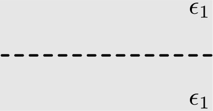
Figure 1: Illustration of a 2D material (dashed line) embedded in a dielectric with dielectric constant $\epsilon_{1}$.

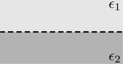
Figure 2: Illustration of a 2D material (dashed line) in the interface between two dielectrics with dielectric constants $\epsilon_{1}$ and $\epsilon_{2}$.

Although Eq. (1) can be applied even when the 2D material is in the interface between two dielectrics with dielectric constants $\epsilon_{1}$ and $\epsilon_{2}$ [making $\epsilon_{1}\to(\epsilon_{1}+\epsilon_{2})/2$ in Eq. (1)], as illustrated in Fig. 2, this formula is unable to address the situation where the 2D material is at a distance $z_{0}$ from the interface (as illustrated in Fig. 3). In the present paper, we investigate, in the context of the cavity PQED, the effect of a planar interface, separating two nondispersive semi-infinite dielectrics ($\epsilon_{1}$ and $\epsilon_{2}$), on the renormalization of the mass (band gap) in a planar 2D material located at a distance $z_{0}$ from the interface (Fig. 3). When $z_{0}=0$ (Fig. 2) or $\epsilon_{1}=\epsilon_{2}$ (Fig. 1), the formula to be obtained here recovers Eq. (1) found in Ref. [35].

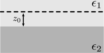
Figure 3: Illustration of a 2D material (dashed line) near to the flat interface between two dielectrics with dielectric constants $\epsilon_{1}$ and $\epsilon_{2}$. The distance between the material and the interface is $z_{0}$, and the 2D material is immersed in the medium with dielectric constant $\epsilon_{1}$.

This paper is organized as follows. In Sec. II, we present the model and its Feynman rules. In Sec. III, we calculate the photon propagator considering the influence of the dielectrics and, subsequently, we incorporate the effects of the polarization tensor into this propagator. In Sec. IV, we calculate the electron self-energy at one-loop order in RPA. In Section V, we obtain the renormalization group functions based on the findings from the preceding section, and we derive the renormalization of the band gap within the framework of the RPA. In Sec. VI, we apply our result to investigate the renormalization of the band gap for a monolayer of WSe₂, when this 2D system is situated within a boron nitride substrate, with a distance $z_{0}$ separating it from the vacuum interface, or conversely, when it is located within the vacuum with a distance $z_{0}$ from the interface of a boron nitride substrate. Finally, in Sec. VII we present our final remarks. We also include an Appendix with some details of the calculations regarding the gauge field propagator in the static regime when dielectrics are present.

II The model and the Feynman Rules

The effective theory and complete description in $2+1$ dimensions for electronic systems moving on a plane, but interacting as particles in $3+1$ dimensions is given by [23]

$$\mathcal{L}_{\mathrm{PQED}}=\frac{1}{2}\frac{{F}_{\mu\nu}{F}^{\mu\nu}}{(-\square)^{1/2}}+\mathcal{L}_{\text{D}}+j^{\mu}A_{\mu}-\frac{\xi}{2}{A}_{\mu}\frac{\partial^{\mu}\partial^{\nu}}{(-\square)^{1/2}}A_{\nu},$$ (3)

where $\square$ is the d’Alembertian operator, $F^{\mu\nu}$ is the usual field intensity tensor of the gauge field $A_{\mu}$ and we consider $c=\hbar=1$. To emulate 2D materials, we shall consider an anisotropic version of the Dirac Lagrangian given by $\mathcal{L}_{\mathrm{D}}=\bar{\psi}_{a}\left(i\gamma^{0}\partial_{0}+iv_{F}\boldsymbol{\gamma}\cdot\nabla\right)\psi_{a}$, where $\bar{\psi}_{a}=\psi^{\dagger}_{a}\gamma^{0}$, and $a=1,\dots,N$ is a flavor index representing a sum over valleys $K$ and $K^{\prime}$, $\gamma^{\mu}$ are rank-4 Dirac matrices and $\psi^{\dagger}_{a}=\big{(}\psi^{\star}_{A\uparrow}\;\psi^{\star}_{A\downarrow}\;\psi^{\star}_{B\uparrow}\;\psi^{\star}_{B\downarrow}\big{)}_{a}$ is a four-component Dirac spinor representing electrons in sublattices $A$ and $B$ in two-dimensional system, with different spin orientations. The last term corresponds to the gauge fixing term.

From Eq. (3), one obtains the free photon propagator in Euclidean space,

$$\Delta_{\mu\nu}^{(0)}(k)=\frac{1}{2\sqrt{k^{2}}}\left[\delta_{\mu\nu}-\left(1-\frac{1}{\xi}\right)\frac{k_{\mu}k_{\nu}}{k^{2}}\right],$$ (4)

where $k_{\mu}=(k_{0},\mathbf{k})$ and $\mathbf{k}=(k_{1},k_{2})$. In the nonretarded regime, considering the Feynman gauge ($\xi=1$), it becomes

$$\Delta_{\mu\nu}^{(0)}(k_{0}=0,|\mathbf{k}|)=\frac{1}{2|\mathbf{k}|}\delta_{0\mu}\delta_{0\nu},$$ (5)

which leads to the Coulombian potential for static charges (instead of the peculiar logarithmic one from QED in $2+1$ dimensions),

$$V(|\mathbf{r}|)=\frac{e}{4\pi}\frac{1}{|\mathbf{r}|}.$$ (6)

The fermion propagator is

$$S_{F}^{(0)}(k^{\mu})=\frac{k_{0}\gamma_{0}+v_{F}\mathbf{k}\cdot\boldsymbol{\gamma}+m}{k_{0}^{2}+v_{F}^{2}|\mathbf{k}|^{2}+m^{2}},$$ (7)

and the vertex interactions is $\gamma^{\mu}=(\gamma^{0},v_{F}\gamma^{i})$.

In this paper, we consider a planar 2D material in a dielectric medium with dielectric constant $\epsilon_{1}$. The 2D material is separated by a distance $z_{0}$ from a parallel interface with another dielectric medium with dielectric constant $\epsilon_{2}$ (see Figs. 3 and 4).

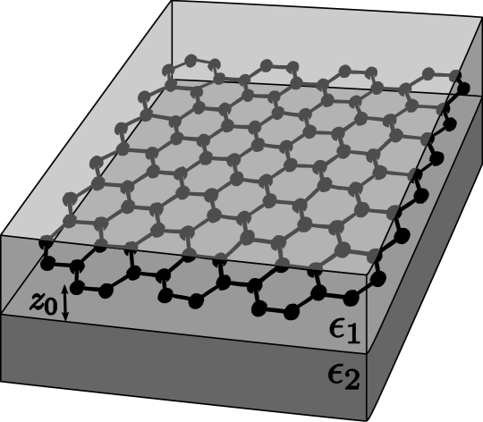
Figure 4: Illustration of a 2D material parallel and near to the interface between two dielectrics with dielectric constants $\epsilon_{1}$ and $\epsilon_{2}$. The distance between the material and the interface is $z_{0}$, the 2D material is immersed in the medium with dielectric constant $\epsilon_{1}$.

III The photon propagator

The gauge-field propagator in the static regime, considering the two dielectric media, is given by (see the Appendix)

$$\Delta_{00}^{(0)}(\left|\mathbf{k}\right|)=\frac{1}{2\epsilon_{1}\sqrt{|\mathbf{k}|^{2}}}\left[1-\frac{\epsilon_{2}-\epsilon_{1}}{\epsilon_{2}+\epsilon_{1}}\exp{\left(-2z_{0}|\mathbf{k}|\right)}\right].$$ (8)

In the following, we shall use this equation to obtain the new expression for the propagator in the large $N$ expansion.

III.1 Photon propagator in large $N$ expansion

We consider the large $N$ expansion at one-loop order approximation, which is equivalent to the RPA [38, 39]. This approximation has been used in the description of some properties of suspended [40, 41] and doped [42, 43, 44] graphene. It can be conveniently implemented by replacing $e\rightarrow e/\sqrt{N}$, for a fixed $e$.

We will consider the geometric series to calculate the full propagator of the gauge-field. Assuming that the interaction vertex is just given by $\gamma_{0}$ (static regime), as illustrated in the Fig. 5,

Figure 5: Gauge field propagator in dominant order in the $1/N$ expansion.

we can write

$$\Delta_{00}^{\mathrm{RPA}}(k)=\Delta_{00}^{(0)}\left(1-\Pi^{00}\Delta_{00}^{(0)}\right),$$ (9)

where [35]

$$\Pi^{00}=-\frac{e^{2}}{8}\left[\frac{|\mathbf{k}|^{2}}{\sqrt{k_{0}^{2}+v_{F}^{2}\mathbf{k}^{2}}}-\frac{4|\mathbf{k}|^{2}m^{2}}{(k_{0}^{2}+v_{F}^{2}|\mathbf{k}|^{2})^{3/2}}\right].$$ (10)

Therefore, we find

$$\Delta_{00}^{\mathrm{RPA}}(k) = \frac{1}{2\epsilon_{1}|\mathbf{k}|}\left\{\frac{1}{1-\kappa_{21}\exp(-2z_{0}|\mathbf{k}|)}+\frac{1}{16}\frac{e^{2}}{\epsilon_{1}}\right.$$

$$\left.\times\left[\frac{|\mathbf{k}|}{\sqrt{k_{0}^{2}+v_{F}^{2}\mathbf{k}^{2}}}-\frac{4|\mathbf{k}|m^{2}}{(k_{0}^{2}+v_{F}^{2}|\mathbf{k}|^{2})^{3/2}}\right]\right\}^{-1}.$$

where we defined

$$\kappa_{21}=\frac{\epsilon_{2}-\epsilon_{1}}{\epsilon_{2}+\epsilon_{1}}.$$ (12)

Note that, in the particular case where $\epsilon_{1}=\epsilon_{2}$ in Eq. (LABEL:propagador-RPA) our model recovers the case of the full propagator of the gauge-field within a single medium [35].

IV Electron self-energy

Considering the static approximation, the electron self-energy, represented in Fig. 6, reads

$$\Sigma(p)=\frac{e^{2}}{N}\int\frac{\mathrm{d}^{3}k}{(2\pi)^{3}}\gamma_{0}S_{F}^{(0)}(p_{\mu}-k_{\mu})\gamma_{0}\Delta_{00}^{\mathrm{RPA}}(k).$$ (13)

Figure 6: Electron self-energy diagram.

Assuming that the Dirac matrices satisfy $\{\gamma^{\mu},\gamma^{\nu}\}=-2\delta^{\mu\nu}$, $\gamma^{0}\gamma^{0}=-\mathbb{I}$ and $\gamma^{0}\boldsymbol{\gamma}\gamma^{0}=\boldsymbol{\gamma}$, and performing a power series expansion in the external momentum, we obtain

$$\Sigma(p)=\mathcal{Z}_{m}+\mathcal{Z}_{0}\gamma_{0}p_{0}+v_{F}\mathcal{Z}_{1}\gamma_{i}p_{i},$$ (14)

where the dominant terms are

$$\mathcal{Z}_{m}=-\frac{e^{2}}{N}\int\frac{\mathrm{d}^{3}k}{(2\pi)^{3}}\frac{m}{k^{2}+m^{2}}\Delta_{00}^{\mathrm{RPA}}(k),$$ (15)

$$\mathcal{Z}_{0}=-\frac{e^{2}}{N}\int\frac{\mathrm{d}^{3}k}{(2\pi)^{3}}\frac{v_{F}^{2}\left|\mathbf{k}\right|^{2}-k_{0}^{2}+m^{2}}{(k^{2}+m^{2}){}^{2}}\Delta_{00}^{\mathrm{RPA}}(k),$$ (16)

and

$$\mathcal{Z}_{1}=\frac{e^{2}}{N}\int\frac{\mathrm{d}^{3}k}{(2\pi)^{3}}\frac{k_{0}^{2}+m^{2}}{\left(k^{2}+m^{2}\right)^{2}}\Delta_{00}^{\mathrm{RPA}}(k).$$ (17)

Then, we perform a variable change $v_{F}k_{i}\rightarrow\bar{k}_{i}$ in Eq. (14) to spherical coordinates, the lowest-order terms can be written as

$$\mathcal{Z}_{m}=-\frac{2\bar{\lambda}}{\pi{}^{2}N}\int_{0}^{\pi}\mathrm{d}\theta\int_{0}^{\Lambda v_{F}}k\,\mathrm{d}k\frac{m}{k^{2}+m^{2}}f(k,\theta),$$ (18)

$$\mathcal{Z}_{0}=\frac{2\bar{\lambda}}{\pi{}^{2}N}\int_{0}^{\pi}\mathrm{d}\theta\int_{0}^{\Lambda v_{F}}k\,\mathrm{d}k\frac{k^{2}(1-2\sin^{2}\theta)-m^{2}}{(k^{2}+m^{2})^{2}}f(k,\theta),$$ (19)

$$\mathcal{Z}_{1}=\frac{2\bar{\lambda}}{\pi{}^{2}N}\int_{0}^{\pi}\mathrm{d}\theta\int_{0}^{\Lambda v_{F}}k\,\mathrm{d}k\frac{k^{2}\cos^{2}\theta+m^{2}}{(k^{2}+m^{2})^{2}}f(k,\theta),$$ (20)

where $\bar{\lambda}=e^{2}/16\epsilon_{1}v_{F}$ and we introduced an ultraviolet cut-off $\Lambda v_{F}$ in the integrals above. We also defined

$$f(k,\theta) = \left\{[1-\kappa_{21}\exp(-2z_{0}k\sin\theta/v_{F})]^{-1}\right.$$ (21)

$$\left.+\bar{\lambda}\left(1-4m^{2}/k^{2}\right)\sin\theta\right\}^{-1}.$$

V Renormalization Group functions

The renormalization group equation reads

$$\bigg{(}\sum_{a}\beta_{a}\frac{\partial}{\mathrm{\partial}a}-N_{F}\gamma_{\psi}-N_{A_{\mu}}\gamma_{A_{\mu}}\bigg{)}\Gamma^{(N_{F},N_{A_{\mu}})}=0,$$ (22)

where $\beta_{a}=\Lambda(\partial a/\partial\Lambda)$, with $a=\{\Lambda,e,v_{F},c,m\}$, are the beta functions of the parameters $e$, $v_{F}$, $c$, and $m$. $N_{F}$ and $N_{A_{\mu}}$ mean the external lines of fermions and $A_{\mu}$ field, respectively. The terms $\gamma_{\psi}$ and $\gamma_{A_{\mu}}$ are the anomalous dimension of the fermion and gauge field, respectively. However, since the polarization tensor for the gauge field is finite at one-loop (using the dimensional regularization), we can conclude that $\gamma_{A_{\mu}}=0$, therefore $\beta_{e}=0$. Thus, for our purpose, we just need to compute the vertex function for the fermion, and thus, the renormalization group equation for $\Gamma^{(2,0)}$ becomes

$$\left(\Lambda\frac{\partial}{\partial\Lambda}+\beta_{v_{F}}\frac{\partial}{\mathrm{\partial}v_{F}}+\beta_{m}\frac{\partial}{\mathrm{\partial}m}-2\gamma_{\psi}\right)\Gamma^{(2,0)}=0,$$ (23)

On the other hand, the vertex function $\Gamma^{(2,0)}$ can be written as

$$\Gamma^{(2,0)}=\gamma_{0}p_{0}+v_{F}\gamma_{i}p_{i}-m+\Sigma(p).$$ (24)

Substituting Eq. (24) into (23) and grouping the terms order by order in the $1/N$ expansion, with $\beta_{a}=N^{0}\beta_{a}^{(0)}+(1/N)\beta_{a}^{(1)}+\cdots$ and $\gamma_{\psi}=N^{0}\gamma_{\psi}^{(0)}+(1/N)\gamma_{\psi}^{(1)}+\cdots$, we obtain

$$\beta_{v_{F}}=\frac{v_{F}\varUpsilon}{N}\int_{0}^{\pi}\mathrm{d}\theta\frac{2m^{2}+\Lambda^{2}v_{F}^{2}\sin^{2}\theta}{(\Lambda^{2}v_{F}^{2}+m^{2})^{2}}f(\theta,\Lambda v_{F}),$$ (25)

$$\beta_{m}=\frac{2m\varUpsilon}{N}\int_{0}^{\pi}\mathrm{d}\theta\frac{\Lambda^{2}v_{F}^{2}\sin^{2}\theta+m^{2}}{(\Lambda^{2}v_{F}^{2}+m^{2})^{2}}f(\theta,\Lambda v_{F}),$$ (26)

$$\gamma_{\psi}=\frac{\varUpsilon}{N}\int_{0}^{\pi}\mathrm{d}\theta\frac{\Lambda^{2}v_{F}^{2}(2\sin^{2}\theta-1)+m^{2}}{(\Lambda^{2}v_{F}^{2}+m^{2})^{2}}f(\theta,\Lambda v_{F}).$$ (27)

where we defined $\varUpsilon=-2\bar{\lambda}(\Lambda v_{F}/\pi)^{2}$.

In the next subsection we will focus only on the analysis of the band gap renormalization.

V.1 Running mass

To calculate the renormalized mass, we use the small-mass limit ($m^{2}\ll\Lambda^{2}v_{F}^{2}$) to neglected the term $4m^{2}/(\Lambda^{2}v_{F}^{2})$ in Eq. (26), and using the definition $\beta_{m}$, we get

$$m=m_{0}\exp\left[\int_{\Lambda_{0}}^{\Lambda}\frac{\mathrm{d}\Lambda}{\Lambda}C_{\bar{\lambda}}(\Lambda)\right],$$ (28)

where

$$C_{\bar{\lambda}}(\Lambda) = -\frac{4\bar{\lambda}}{\pi{}^{2}N}\int_{0}^{\pi}\mathrm{d}\theta\sin^{2}\theta$$ (29)

$$\times\left[\frac{1}{1-\kappa_{21}\exp(-2z_{0}\Lambda\sin\theta)}+\bar{\lambda}\sin\theta\right]^{-1}.\qquad$$

For a two-dimensional system, we can show that the carrier concentration $n=N_{e}/A$, where $N_{e}$ is the number of electrons and $A$ is the area occupied by each state, can be written as $n=N_{e}/A=p^{2}_{F}/\pi$ [45, 46]. Therefore, it follows that the Fermi momentum reads $p_{F}=(\pi n)^{1/2}$. This plays the role of our energy scale $\Lambda$, thus, we shall use the transformation $\Lambda/\Lambda_{0}\rightarrow(n/n_{0})^{1/2}$ for our renormalized functions.

We remark that, for $\epsilon_{2}=\epsilon_{1}$ (situation illustrated in Fig. 1), Eqs. (28) and (29) recover Eqs. (1) and (2) found in the literature [35]. For $z_{0}=0$ (situation illustrated in Fig. 2), Eqs. (28) and (29) give Eqs. (1) and (2), with $\epsilon_{1}\to(\epsilon_{1}+\epsilon_{2})/2$.

VI Application

Here, we apply our formulas to investigate the renormalization of the band gap for a monolayer of WSe₂, when this 2D system is inside a boron nitride substrate ($\epsilon_{1}=4$), at a distance $z_{0}$ from an interface with the vacuum ($\epsilon_{2}=1$) (see Figs. 3 and 4). We also investigate the opposite situation when the monolayer of WSe₂ is inside the vacuum ($\epsilon_{1}=1$), at a distance $z_{0}$ from the interface with the boron nitride substrate ($\epsilon_{2}=4$). Taking Refs. [35, 36] as basis, we consider the reference values $n_{0}=1.58\times 10^{12}\text{c}\text{m}^{-2}$, $\bar{\lambda}=0.48$ (when $\epsilon_{1}=4$), and $\bar{\lambda}=1.92$ (when $\epsilon_{1}=1$). Using Eq. (28) and putting the flavor number $N=2$ due to the degeneracy of the valleys $K$ and $K^{\prime}$, we obtain the behavior of $m/m_{0}$ as function of $n$, for several situations discussed next, always comparing our results with those obtained if Eq. (1) (found in Ref. [35]) were applied as if the 2D system were in a single medium $\epsilon_{1}$.

In Fig. 7(a), we show the ratio $m/m_{0}$ versus $n$, for a monolayer of WSe₂ inside a boron nitride substrate ($\epsilon_{1}=4$), at a distance $z_{0}=100\text{nm}$ from an interface with the vacuum. The solid (blue) line shows the curve obtained via Eq. (28), whereas the dashed (orange) line shows the curve obtained via Eq. (1), this latter applied as if the WSe₂ were immersed in an infinite boron nitride substrate, ignoring the interface with the vacuum. It is evident that Eq. (1) overestimates the values of $m/m_{0}$ for $n>n_{0}$ in comparison to the precise values obtained from Eq. (28), whereas it predicts lower values for $n<n_{0}$. On the other hand, this difference decreases as $z_{0}$ increases, as expected and shown in Fig. 7(b) (for $z_{0}=300\text{nm}$) and Fig. 7(c) (for $z_{0}=500\text{nm}$).

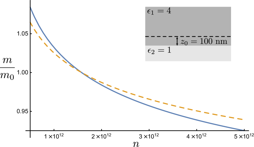
(a) $z_{0}=100\text{nm}$.

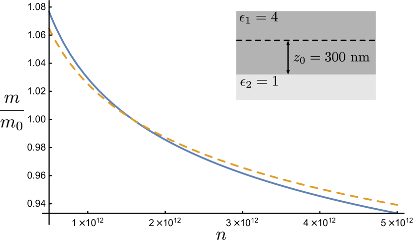
(b) $z_{0}=300\text{nm}$.

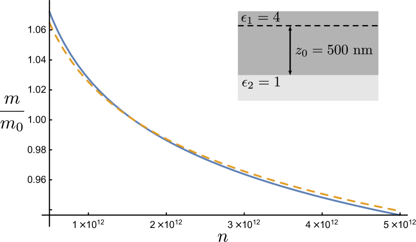
(c) $z_{0}=500\text{nm}$.

Figure 7: Ratio $m/m_{0}$ as function of $n$, for a monolayer of WSe₂ inside a boron nitride substrate ($\epsilon_{1}=4$) near the interface with the vacuum ($\epsilon_{2}=1$), for different values of $z_{0}$. The solid (blue) and dashed (orange) lines show the curves obtained via Eqs. (28) and (1), respectively.

In Fig. 8, we show the situation where the media are interchanged, i.e. the monolayer of WSe₂ is inside vacuum ($\epsilon_{1}=1$), at a distance $z_{0}$ from the interface with the boron nitride substrate ($\epsilon_{2}=4$). In Fig. 8(a), we show the ratio $m/m_{0}$ versus $n$ for $z_{0}=100\text{nm}$. The solid (blue) line shows the curve obtained via Eq. (28), whereas the dashed (orange) line shows the curve obtained via Eq. (1), this latter applied as if the WSe₂ were immersed in an infinite vacuum, ignoring the interface with the boron nitride substrate. One can see that Eq. (1) predicts lower values for $m/m_{0}$ in comparison to the precise values obtained from Eq. (28), whereas it predicts higher values for $n<n_{0}$. On the other hand, this difference decreases as $z_{0}$ increases, as expected and shown in Fig. 8(b) (for $z_{0}=300\text{nm}$) and Fig. 8(c) (for $z_{0}=500\text{nm}$).

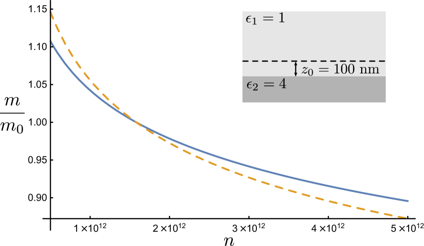
(a) $z_{0}=100\text{nm}$.

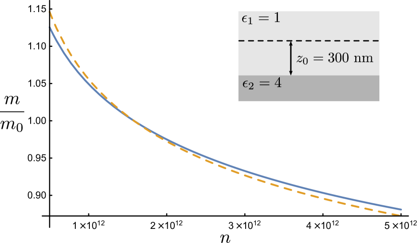
(b) $z_{0}=300\text{nm}$.

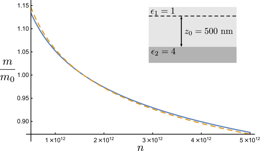
(c) $z_{0}=500\text{nm}$.

Figure 8: Ratio $m/m_{0}$ as function of $n$ in the opposite situation to that shown in Fig. 7. Here the monolayer of WSe₂ is inside vacuum ($\epsilon_{1}=1$) and near to the interface with a boron nitride substrate ($\epsilon_{2}=4$). The solid (blue) and dashed (orange) lines show the curves obtained via Eqs. (28) and (1), respectively.

VII Final Remarks

We investigated, in the context of the cavity PQED and considering the RPA, the effect of a planar interface (between two nondispersive semi-infinite dielectrics) on the renormalization of the mass (band gap) in a planar 2D material located at a distance $z_{0}$ from the interface (Fig. 3). Our result [Eq. (28)] enables us to predict the behavior of the band gap as a function of the density of states, under the influence of such interface.

As an application, we considered Eq. (28) to investigate the renormalization of the band gap for a monolayer of WSe₂, when this 2D system is inside a boron nitride substrate, at a distance $z_{0}$ from an interface with the vacuum (see Fig. 7). We also investigated the opposite situation when the WSe₂ is inside vacuum, at a distance $z_{0}$ from the interface with the boron nitride substrate (see Fig. 8). We compared our results with those obtained if Eq. (1) (found in Ref. [35]) were applied as if the 2D system were in a single medium. The differences between the more precise predictions, given by our Eq. (28), and those obtained by Eq. (1) are larger for smaller values of $z_{0}$ [see Figs. 7(a) and 8(a)], which means that the effect of the interface, captured by Eq. (28), is significant. On the other hand, as $z_{0}$ increases, the differences decrease [see Figs. 7(c) and 8(c)], which means that the effect of the interface on the renormalized band gap becomes small for larger distances $z_{0}$, as expected.

Since experiments verifying the dependence of the band gap with the density of states have been made [36, 37], an experimental verification of the effects predicted here, according to Eq. (28), seems feasible.

Appendix A Photon propagator

Consider an electric charge $e$ in a semi-infinity dielectric medium with dielectric constant $\epsilon_{1}$ separated by a distance $z_{0}$ from the interface between another semi-infinity dielectric medium with dielectric constant $\epsilon_{2}$. By the image method, the potential $V$ for this configuration at an arbitrary point $P$ (also separated by a distance $z_{0}$ from the interface) is (see Fig. 9)

$$V(|\mathbf{r}|)=\frac{1}{4\pi\epsilon_{1}}\left(\frac{e}{|\mathbf{r}|}+\frac{e^{\prime}}{|\mathbf{r}^{\prime}|}\right),$$ (30)

where $|\mathbf{r}|$ is the distance between the charge $e$ and the point $P$ and $|\mathbf{r}^{\prime}|$ is the distance between the image charge $e^{\prime}$ and the point $P$. The image charge $e^{\prime}$ given by

$$e^{\prime}=-\kappa_{21}e,$$ (31)

and the distance between the image charge and the point $P$ is $|\mathbf{r^{\prime}}|=\sqrt{|\mathbf{r}|^{2}+4z_{0}^{2}}$. Therefore, the potential at $P$ is

$$V(|\mathbf{r}|)=\frac{e}{4\pi\epsilon_{1}}\left(\frac{1}{|\mathbf{r}|}-\frac{\kappa_{21}}{\sqrt{|\mathbf{r}|^{2}+4z_{0}^{2}}}\right).$$ (32)

From this static potential, via the inverse Fourier transform, which is given by (see, for instance, Ref. [47])

$$\Delta_{00}^{(0)}(|\mathbf{k}|)=\frac{1}{e^{2}}\int\mathrm{d}^{2}\mathbf{r}\,\mathrm{e}^{-i\mathbf{k}\cdot\mathbf{r}}eV(|\mathbf{r}|),$$ (33)

where $k_{0}=0$, and $\mathbf{k}$ and $\mathbf{r}$ are restricted to the plane $z=z_{0}$, thus we can write $\mathbf{k}\cdot\mathbf{r}=|\mathbf{k}||\mathbf{r}|\cos\varphi$ and $\mathrm{d}^{2}\mathbf{r}=|\mathbf{r}|\,\mathrm{d}\varphi\,\mathrm{d}|\mathbf{r}|$. After performing the integration, we obtain Eq. (8). The first term is the propagator in the absence of the medium with $\epsilon_{2}$ (recovered when $z_{0}\rightarrow\infty$), and the exponential term arises due to the presence of the medium with $\epsilon_{2}$.

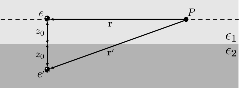
Figure 9: An electric charge $e$ and its image $e^{\prime}$, each one separated by a distance $z_{0}$ from the interface between the two dielectric media. The charge $e$ is in the medium with dielectric constant $\epsilon_{1}$ and its image is in the medium with dielectric constant $\epsilon_{2}$. $P$ is an arbitrary point of the plane that contains the charge $e$ and it is parallel to the interface.

References

- Maris [1994] P. Maris, Analytic structure of the full fermion propagator in quenched and unquenched QED, Phys. Rev. D 50, 4189 (1994).
- Appelquist et al. [1985] T. Appelquist, M. J. Bowick, E. Cohler, and L. C. R. Wijewardhana, Chiral-symmetry breaking in 2+1 dimensions, Phys. Rev. Lett. 55, 1715 (1985).
- Burden et al. [1992] C. J. Burden, J. Praschifka, and C. D. Roberts, Photon polarization tensor and gauge dependence in three-dimensional quantum electrodynamics, Phys. Rev. D 46, 2695 (1992).
- Grignani et al. [1996] G. Grignani, G. Semenoff, and P. Sodano, Confinement-deconfinement transition in three-dimensional QED, Phys. Rev. D 53, 7157 (1996).
- Maris [1995] P. Maris, Confinement and complex singularities in three-dimensional QED, Phys. Rev. D 52, 6087 (1995).
- Prange and Girvin [1990] R. E. Prange and S. M. Girvin, eds., The Quantum Hall effect (Springer, New York, 1990).
- Wilczek [1990] F. Wilczek, Fractional statistics and anyon superconductivity, Vol. 5 (World scientific, Singapore, 1990).
- Halperin [1982] B. I. Halperin, Quantized Hall conductance, current-carrying edge states, and the existence of extended states in a two-dimensional disordered potential, Phys. Rev. B 25, 2185 (1982).
- Laughlin [1981] R. B. Laughlin, Quantized Hall conductivity in two dimensions, Phys. Rev. B 23, 5632 (1981).
- Laughlin [1988] R. B. Laughlin, Superconducting ground state of noninteracting particles obeying fractional statistics, Phys. Rev. Lett. 60, 2677 (1988).
- Chen et al. [1989] Y.-H. Chen, F. Wilczek, E. Witten, and B. I. Halperin, On anyon superconductivity, International Journal of Modern Physics B 03, 1001 (1989).
- Geim and Novoselov [2007] A. K. Geim and K. S. Novoselov, The rise of graphene, Nature materials 6, 183 (2007).
- Radisavljevic et al. [2011] B. Radisavljevic, A. Radenovic, J. Brivio, V. Giacometti, and A. Kis, Single-layer MoS2 transistors, Nature nanotechnology 6, 147 (2011).
- Wang et al. [2012] Q. H. Wang, K. Kalantar-Zadeh, A. Kis, J. N. Coleman, and M. S. Strano, Electronics and optoelectronics of two-dimensional transition metal dichalcogenides, Nature nanotechnology 7, 699 (2012).
- Liu et al. [2014] H. Liu, A. T. Neal, Z. Zhu, Z. Luo, X. Xu, D. Tománek, and P. D. Ye, Phosphorene: An unexplored 2D semiconductor with a high hole mobility, ACS Nano 8, 4033 (2014).
- Castro Neto et al. [2009] A. H. Castro Neto, F. Guinea, N. M. R. Peres, K. S. Novoselov, and A. K. Geim, The electronic properties of graphene, Rev. Mod. Phys. 81, 109 (2009).
- Elias et al. [2011] D. C. Elias, R. V. Gorbachev, A. S. Mayorov, S. V. Morozov, A. A. Zhukov, P. Blake, L. A. Ponomarenko, I. V. Grigorieva, K. S. Novoselov, F. Guinea, and A. K. Geim, Dirac cones reshaped by interaction effects in suspended graphene, Nat. Phys. 7, 701 (2011).
- Du et al. [2008] X. Du, I. Skachko, A. Barker, and E. Y. Andrei, Approaching ballistic transport in suspended graphene, Nature nanotechnology 3, 491 (2008).
- Du et al. [2009] X. Du, I. Skachko, F. Duerr, A. Luican, and E. Y. Andrei, Fractional quantum Hall effect and insulating phase of Dirac electrons in graphene, Nature 462, 192 (2009).
- Bolotin et al. [2009] K. I. Bolotin, F. Ghahari, M. D. Shulman, H. L. Stormer, and P. Kim, Observation of the fractional quantum Hall effect in graphene, Nature 462, 196 (2009).
- Ghahari et al. [2011] F. Ghahari, Y. Zhao, P. Cadden-Zimansky, K. Bolotin, and P. Kim, Measurement of the fractional quantum Hall energy gap in suspended graphene, Phys. Rev. Lett. 106, 046801 (2011).
- Dean et al. [2011] C. R. Dean, A. F. Young, P. Cadden-Zimansky, L. Wang, H. Ren, K. Watanabe, T. Taniguchi, P. Kim, J. Hone, and K. Shepard, Multicomponent fractional quantum Hall effect in graphene, Nature Physics 7, 693 (2011).
- Marino [1993] E. Marino, Quantum electrodynamics of particles on a plane and the Chern-Simons theory, Nuclear Physics B 408, 551 (1993).
- Gorbar et al. [2001] E. V. Gorbar, V. P. Gusynin, and V. A. Miransky, Dynamical chiral symmetry breaking on a brane in reduced qed, Phys. Rev. D 64, 105028 (2001).
- Marino et al. [2014] E. C. Marino, L. O. Nascimento, V. S. Alves, and C. Morais Smith, Unitarity of theories containing fractional powers of the d’Alembertian operator, Physical Review D 90, 105003 (2014).
- do Amaral and Marino [1992] R. L. P. G. do Amaral and E. C. Marino, Canonical quantization of theories containing fractional powers of the d’Alembertian operator, Journal of Physics A: Mathematical and General 25, 5183 (1992).
- Dudal et al. [2019] D. Dudal, A. J. Mizher, and P. Pais, Exact quantum scale invariance of three-dimensional reduced QED theories, Phys. Rev. D 99, 045017 (2019).
- Heydeman et al. [2020] M. Heydeman, C. B. Jepsen, Z. Ji, and A. Yarom, Renormalization and conformal invariance of non-local quantum electrodynamics, Journal of High Energy Physics 2020, 1 (2020).
- Menezes et al. [2016] N. Menezes, V. S. Alves, and C. M. Smith, The influence of a weak magnetic field in the renormalization-group functions of -dimensional Dirac systems, Eur. Phys. J. B 89, 271 (2016).
- Menezes et al. [2017] N. Menezes, V. S. Alves, E. C. Marino, L. Nascimento, L. O. Nascimento, and C. Morais Smith, Spin -factor due to electronic interactions in graphene, Phys. Rev. B 95, 245138 (2017).
- Marino et al. [2018] E. C. Marino, L. O. Nascimento, V. S. Alves, N. Menezes, and C. M. Smith, Quantum-electrodynamical approach to the exciton spectrum in transition-metal dichalcogenides, 2D Materials 5, 041006 (2018).
- Pedrelli et al. [2020] D. C. Pedrelli, D. T. Alves, and V. S. Alves, Two-loop photon self-energy in pseudoquantum electrodynamics in the presence of a conducting surface, Phys. Rev. D 102, 125032 (2020).
- Silva et al. [2017] J. D. L. Silva, A. N. Braga, W. P. Pires, V. S. Alves, D. T. Alves, and E. C. Marino, Inhibition of the fermi velocity renormalization in a graphene sheet by the presence of a conducting plate, Nucl. Phys. B 920, 221 (2017).
- Pires et al. [2018] W. P. Pires, J. D. L. Silva, A. N. Braga, V. S. Alves, D. T. Alves, and E. C. Marino, Cavity effects on the Fermi velocity renormalization in a graphene sheet, Nucl. Phys. B 932, 529 (2018).
- Fernández et al. [2020] L. Fernández, V. S. Alves, L. O. Nascimento, F. Peña, M. Gomes, and E. C. Marino, Renormalization of the band gap in 2D materials through the competition between electromagnetic and four-fermion interactions in large expansion, Phys. Rev. D 102, 016020 (2020).
- Nguyen et al. [2019] P. V. Nguyen, N. C. Teutsch, N. P. Wilson, J. Kahn, X. Xia, A. J. Graham, V. Kandyba, A. Giampietri, A. Barinov, G. C. Constantinescu, N. Yeung, N. D. M. Hine, X. Xu, D. H. Cobden, and N. R. Wilson, Visualizing electrostatic gating effects in two-dimensional heterostructures, Nature 572, 220 (2019).
- Liu et al. [2019] F. Liu, M. E. Ziffer, K. R. Hansen, J. Wang, and X. Zhu, Direct determination of band-gap renormalization in the photoexcited monolayer , Phys. Rev. Lett. 122, 246803 (2019).
- Vozmediano and Guinea [2012] M. A. H. Vozmediano and F. Guinea, Effect of Coulomb interactions on the physical observables of graphene, Phys. Scr. 2012, 014015 (2012).
- de Juan et al. [2010] F. de Juan, A. G. Grushin, and M. A. H. Vozmediano, Renormalization of coulomb interaction in graphene: Determining observable quantities, Phys. Rev. B 82, 125409 (2010).
- González et al. [1999] J. González, F. Guinea, and M. A. H. Vozmediano, Marginal-fermi-liquid behavior from two-dimensional coulomb interaction, Phys. Rev. B 59, R2474 (1999).
- Kotov et al. [2009] V. N. Kotov, B. Uchoa, and A. H. Castro Neto, expansion in correlated graphene, Phys. Rev. B 80, 165424 (2009).
- Das Sarma et al. [2007] S. Das Sarma, E. H. Hwang, and W.-K. Tse, Many-body interaction effects in doped and undoped graphene: Fermi liquid versus non-fermi liquid, Phys. Rev. B 75, 121406 (2007).
- Polini et al. [2007] M. Polini, R. Asgari, Y. Barlas, T. Pereg-Barnea, and A. MacDonald, Graphene: A pseudochiral fermi liquid, Solid State Communications 143, 58 (2007), exploring graphene.
- Hwang and Das Sarma [2007] E. H. Hwang and S. Das Sarma, Dielectric function, screening, and plasmons in two-dimensional graphene, Phys. Rev. B 75, 205418 (2007).
- Marino [2017] E. C. Marino, Quantum Field Theory Approach to Condensed Matter Physics (Cambridge University Press, Cambridge and New York, 2017).
- Salinas [2013] S. Salinas, Introduction to Statistical Physics, Graduate Texts in Contemporary Physics (Springer New York, 2013).
- Roberts and Williams [1994] C. D. Roberts and A. G. Williams, Dyson-Schwinger equations and their application to hadronic physics, Progress in Particle and Nuclear Physics 33, 477 (1994).