Anomalous Holographic Hard Wall Model for
Glueballs and the Pomeron

Abstract

In this work we propose an improved holographic hard wall (HW) model by the inclusion of anomalous dimensions in the dual operators that describe glueballs inspired by the AdS/CFT correspondence. The anomalous dimensions come from well known gauge/string duality analysis showing a dependence with the logarithm of spin $S$ of the boundary states. We show that this logarithm anomalous dimensions of the high spin operators combined with the usual HW model allow us to match the pomeron trajectory and give glueball masses which are better than that of the original HW in comparison with lattice data. We also build up other HW models considering that the logarithm anomalous dimensions can be approximated by a series of odd powers of the difference $\sqrt{S}-1/\sqrt{S}$. These models fit the pomeron trajectory and produce good glueball masses. Then, we consider an anomalous dimension which is proportional to $\sqrt{S}$, providing reasonable results. Finally, we propose an asymptotic linear HW model which effective dimension for high spins operators are of the form $\Delta=a\sqrt{S}+b$, where $a$ and $b$ are constants to be fixed by comparison with the soft pomeron trajectory and lattice data. This model matches the soft pomeron trajectory with the same significant figures and generates masses with deviations from the lattice under $10\%$.

I Introduction

QCD describes strong interactions. At high energies its coupling is small so that it can be treated perturbatively. On the other side, at low energies, the QCD coupling is large and non-perturbative methods are needed to tackle phenomena like confinement, phase transitions, and hadronic spectra. This non-perturbative behavior usually requires involved numerical calculations known as lattice QCD. Alternatively, low energy QCD may be approached by other methods, as the solution of Schwinger-Dyson equations, QCD sum rules and effective models (for a review see, e. g., Gross:2022hyw ). In particular, models inspired by the AdS/CFT correspondence Aharony:1999ti ; Polchinski:2001tt ; Polchinski:2002jw ; Gubser:2002tv proved useful to describe different aspects of hadrons with various spins, as glueballs Csaki:1998qr ; deMelloKoch:1998vqw ; Hashimoto:1998if ; Csaki:1998cb ; Minahan:1998tm ; Brower:2000rp ; Caceres:2000qe ; Boschi-Filho:2002xih ; Boschi-Filho:2002wdj ; Apreda:2003sy ; Amador:2004pz ; Evans:2005ip ; Caceres:2005yx ; Boschi-Filho:2005xct ; FolcoCapossoli:2013eao , as well as for mesons and baryons, as for instance, in Sakai:2004cn ; Sakai:2005yt ; deTeramond:2005su ; Ghoroku:2005vt ; Erlich:2005qh ; DaRold:2005mxj ; Karch:2006pv ; Brodsky:2006uqa ; Hata:2007mb ; Forkel:2007cm ; Gursoy:2007cb ; Gursoy:2007er ; Erdmenger:2007cm ; dePaula:2008fp ; Vega:2008af ; Abidin:2009hr ; Gutsche:2011vb ; Li:2012ay ; Brodsky:2014yha ; Sonnenschein:2016pim ; FolcoCapossoli:2019imm ; Afonin:2020msa ; Rinaldi:2021dxh .

The holographic hard wall (HW) model Boschi-Filho:2002xih ; Boschi-Filho:2002wdj introduces a hard cutoff in the AdS space, described by Poincaré coordinates

$$ds^{2}=\frac{R^{2}}{z^{2}}(dz^{2}+(d\vec{x})^{2}-dt^{2})$$ (1)

such that the size of the AdS slice, $0\leq z\leq z_{\rm max}$, can be related to a QCD scale, $\Lambda_{\rm QCD}$, as

$$z_{\rm max}=\frac{1}{\Lambda_{\rm QCD}}.$$ (2)

Then, the five dimensional AdS bulk fields are described by Bessel functions of order $\nu$, $J_{\nu}(z)$. The discreteness of the hadronic spectra is assured by imposing boundary conditions at $z=z_{\rm max}$. This way, hadronic masses $M$ are proportional to the zeros of Bessel functions, $J_{\nu}(z)$. This model was inspired by holographic descriptions of hard scattering of glueballs Polchinski:2001tt and deep inelastic scattering of hadrons Polchinski:2002jw , and it is very useful to obtain hadronic form factors, structure functions, parton distribution functions, etc (see, e. g., Grigoryan:2007vg ; Mamo:2021cle ). A well known drawback of the hard wall model is that it leads to non-linear Regge trajectories, $J\times m^{2}$. It is important to mention that in the HW, the order of the Bessel function $\nu$ is related to the conformal dimension of the dual operator. For instance, for even spin $S$ glueballs, it reads $\nu=S+2$ deTeramond:2005su ; Boschi-Filho:2005xct . Actually, in Ref. Boschi-Filho:2005xct , approximate linear Regge trajectories for light even glueballs were obtained $\alpha(t=M^{2})=(0.80\pm 0.40)+(0.26\pm 0.02)M^{2}$ and compared to a reasonable approximation to that of the soft pomeron $\alpha(t=M^{2})=1.08+0.25M^{2}$ Landshoff:2001pp ; Meyer:2004jc . A similar analysis within the HW was done for odd spin glueballs comparing their Regge trajectories with the odderon FolcoCapossoli:2013eao , and also for other hadrons with different spins deTeramond:2005su ; Erlich:2005qh .

In this work, we consider the inclusion of anomalous dimensions in the conformal dimension of boundary operators in the holographic hard wall model. As is well known Gross:2022hyw , anomalous dimensions appear in QCD loop corrections, as in the BFKL pomeron Fadin:1998py , as well as in a semi-classical limit of gauge/string dualities Gubser:2002tv . As we show here, the introduction of anomalous dimensions in the HW model lead to improvements of the model allowing the match of the Regge trajectory of the pomeron with the same significant figures. In particular, we also show that considering the dimension of the spin $S$ operators as $\Delta=a\sqrt{S}+b$, where $a$ and $b$ are constants, imply an asymptotic linear Regge trajectory associated with even glueballs. The glueball masses obtained from these anomalous models are better than that of the original HW when compared with lattice data.

This work is organized as follows. In section II, we briefly review the original HW model applied to even glueballs, and in Section II.1 introduce the anomalous HW model. In Section III we discuss various anomalous HW models and compare them to the pomeron trajectory and to the lattice data for glueball masses. In particular, in Section III.1 we study logarithm anomalous dimensions, followed by Section III.2 where we consider HW models with some approximations for the logarithm anomalous dimensions, and in Section III.3, we analyse a HW model with square root anomalous dimensions. Then, in Section IV we propose an asymptotic linear HW model fitting the pomeron trajectory and presenting good glueball masses compared with lattice data. Finally, in Section V we present our conclusions.

II The Original and the Anomalous Hard Wall Models

The hard wall model Boschi-Filho:2002xih ; Boschi-Filho:2002wdj consists of fields defined in the bulk of a slice of the AdS space, $0\leq z\leq z_{\rm max}$ with metric, Eq. (1), and action

$$\int dzd^{4}x\sqrt{-g}\,{\cal L},$$ (3)

where $\cal L$ is the Lagrangian of the fields. The solutions for scalar fields with mass $\mu$ satisfy

$$\Big{[}z^{3}\partial_{z}\frac{1}{z^{3}}\partial_{z}\,+\,\eta^{\mu\nu}\partial_{\mu}\partial_{\nu}\,-\,\frac{(\mu R)^{2}}{z^{2}}\,\,\Big{]}\,\phi\,\,=\,\,0\,\,.$$ (4)

According to the AdS/CFT correspondence Aharony:1999ti , these fields are dual to boundary operators $\cal O$ with dimension $\Delta$ such that

$$\Delta=2+\sqrt{4+(\mu R)^{2}}\,\,.$$ (5)

From this relation for scalar fields, one finds that Eq. (4) becomes

$$\Big{[}z^{3}\partial_{z}\frac{1}{z^{3}}\partial_{z}\,+\,\eta^{\mu\nu}\partial_{\mu}\partial_{\nu}\,-\,\frac{\Delta(\Delta-4)}{z^{2}}\,\,\Big{]}\,\phi\,\,=\,\,0\,\,.$$ (6)

Considering free particle plane waves in four dimensional Minkowski coordinates $x^{\mu}=(t,\vec{x})$, one can write the solutions for this equation as

$$\phi\,(x,z)\,=\,C_{\nu,k}\,e^{-iP\cdot x}\,z^{2}J_{\nu}(u_{\nu,k}\,\,z\,)\,,$$ (7)

where $J_{\nu}(w)$ are Bessel functions of order $\nu$, with $\nu=\Delta-2$, and the discrete modes $u_{\nu,k}\,$ ($k=1,2,...)\,$ are determined by boundary conditions to be imposed at $z=z_{\rm max}$. For Dirichlet boundary conditions $\phi(x,z)|_{\,z=z_{\rm max}}=0$, one finds that the discrete modes $u_{\nu,k}\,$ ($k=1,2,...)\,$ are given by

$$u_{\nu,k}\,=\,\frac{\chi_{{}_{\nu,k}}}{z_{\rm max}}\,=\,\chi_{{}_{\nu,k}}\,\Lambda_{\rm QCD}\qquad;\qquad J_{\nu}(\,\chi_{{}_{\nu,k}}\,)\,=\,0\,.$$ (8)

The scale $\Lambda_{\rm QCD}$ is usually fixed using some experimental or lattice data. The $k$ indices label the radial excitations of the particle states with masses proportional to the zeros of the Bessel function $J_{\nu}(w)$.

In particular, scalar glueball states are associated the operator ${\cal O}_{4}={\rm tr}F^{2}$, which have conformal dimension $\Delta=4$, spin $S=0$, implying a twist $\tau=\Delta-S=4$, and are described by massless $(\mu=0)$ five dimensional scalar fields in AdS space. Complementary, twist four high spin $S$ operators can be written as:

$${\cal O}_{4+S}\,=\,{\rm tr}FD_{\{\mu_{1}}...D_{\mu_{S}\,\}}F,$$ (9)

with canonical conformal dimension

$$\Delta_{\rm can.}=4+S.$$ (10)

So, using the above discussion of the HW model, one can calculate higher spin glueball masses from relations (8) and (10) such that with $\nu=\Delta-2=S+2$

$$u_{S+2,k}=\chi_{S+2,k}\,\Lambda_{\rm QCD},$$ (11)

for instance, with the Dirichlet boundary condition $J_{S+2}(\chi_{S+2,k})=0$. Using this relation, one finds the glueball masses from the original HW Boschi-Filho:2005xct , which we are presented here for latter convenience together with the available lattice data Teper:1997am ; Morningstar:1997ff ; Morningstar:1999rf in Table 1, and the corresponding relative errors $\delta_{i}=|M_{\rm latt.}-M_{i}|/M_{\rm latt.}$ In this work we use the mass of the $0^{++}$ glueball state from lattice as an input for all the models considered here.

Table 1: Masses in GeV of the $J^{++}$ glueball operators with even spins available from lattice Teper:1997am ; Morningstar:1997ff ; Morningstar:1999rf , and from the original (HW) hard wall model Boschi-Filho:2005xct from Eq. (11) with canonical conformal dimension Eq. (10). The mass of the $0^{++}$ inserted as an input for the HW model and we also show the percent errors $\delta_{\rm HW}$ relative to lattice data.

$J^{PC}$	Lattice	HW	$\delta_{\rm HW}$
$0^{++}$	$1.59$	$1.59$	$0.0\%$
$2^{++}$	$2.39$	$2.35$	$1.7\%$
$4^{++}$	$3.80$	$3.08$	$19\%$
$6^{++}$	$4.48$	$3.78$	$16\%$
$8^{++}$	-	$4.48$	-
$10^{++}$	-	$5.17$	-

It is important to remark that despite the success of the HW to predict hadronic masses the corresponding Regge trajectories $J\times M^{2}$ are non-linear in contrast with experimental data. One can understand this behavior from the following.

Assuming the duality between the bulk modes in the $AdS_{5}$ slice and the glueball operators, the scalar glueball ground state $0^{++}$ is related to the massless scalar. So its mass is proportional to $\chi_{2,1}$. Fixing $k=1$, for example, we can study how $S$ and $M$ are related. Since (11) relates in a linear way the mass $M$ (proportional to $u$) and the first Bessel function zero of index $S+2$, this zero grows in an asymptotically linear way with $S$, and leads to an inherently non-linear (quadratic) graph $S\times M^{2}$. We will return to this point in section IV, where we propose an asymptotically linear HW model inspired by the anomalous HW model that we introduce now.

II.1 Anomalous Hard Wall Model

Our proposal here, is to include anomalous dimensions in the conformal dimension of the boundary glueball operators, modifying the relation between $\Delta$ and $S$. It is well known that anomalous dimensions play a important role in the renormalization of QCD (see e. g. Gross:2022hyw ) and the BFKL pomeron Fadin:1998py , for instance, however it is difficult to relate it to high spin states.

On the other side, from a semi-classical limit of gauge/string dualities Gubser:2002tv , one finds that the conformal dimension of dual operators with spins $S$, as the ones given in Eq. (9), behave as the canonical dimension, Eq. (10), for low spins $S\ll\sqrt{\lambda}$, some other complicate non-perturbative relation for intermediate values $S\sim\sqrt{\lambda}$, and

$$\Delta=S+\frac{\sqrt{\lambda}}{\pi}\ln\left(\frac{S}{\sqrt{\lambda}}\right)+{\cal{O}}(S^{0}),$$ (12)

for $S\gg\sqrt{\lambda}$, where $\lambda$ is the t’Hooft coupling.

The phenomenological holographic model that we are proposing, is a simplified version of the behavior for various spins described above. For low spins, we assume the canonical dimension Eq. (10), and for high spins the equation (12), without a complicated intermediate regime. The transition between low and high spins will be determined by the best fit to experimental or lattice data. As we are going to see below, this model produces interesting results, improving the ones from the usual hard wall model regarding the predicted masses and the corresponding Regge trajectories.

III Glueballs and the Soft Pomeron in The Anomalous HW

The rise of the proton-proton cross section with energy is related to the soft pomeron, a particle with no charges and quantum numbers of the vacuum, whose experimental Regge trajectory is the following Landshoff:2001pp ; Meyer:2004jc

$$\alpha(t=M^{2})=1.08+0.25M^{2},$$ (13)

with masses $M$ expressed in GeV. The BFKL pomeron Fadin:1998py is a perturbative treatment of the problem, although non-perturbative aspects are also present (see e. g. Lebiedowicz:2023mhe ).

III.1 Logarithm anomalous dimensions

In order to apply the anomalous HW model proposed in the previous section to physical situations determined by experimental and lattice data, we are going to rewrite the effective dimensions for high spins, Eq. (12), as

$$\Delta=S+a\ln{(S)}+b,$$ (14)

where the constants $a$, and $b$ will determined fitting experimental and lattice data below.

In accordance with the anomalous HW proposed in the previous section, we consider that the state $0^{++}$ has canonical conformal dimension $\Delta=4$, and use it as an input with mass $M_{0^{++}}=1.59\mbox{ GeV}$ from lattice. Following Landshoff Landshoff:2001pp , we take that this state does not belong to the soft pomeron trajectory. The transition between low and high spins, given by Eqs. (10) and (14), respectively, will be determined by best fit of the pomeron trajectory, Eq. (13) and taking into account the predicted glueball masses for the states $J^{++}$ from $J=2$ to $J=10$ in comparison with lattice data, using Dirichlet boundary conditions. This procedure will fix the constants $a$, and $b$. This is what we call the HW_log model.

To perform the comparison with the pomeron Regge trajectory and the glueball masses from lattice data, we consider first that Eq. (14) is valid from $J=S=2$ to higher spins. Then, we use this equation to fit the pomeron trajectory. The best fit obtained in this way implies the coefficients $a=1.85$, and $b=2.14$, such that the effective dimension in the anomalous HW_log1 model is given by

$$\Delta_{\rm log1}=S+1.85\ln{(S)}+2.14.$$ (15)

From this anomalous dimension, we obtain the glueball masses shown in Table (2), together with relative errors in comparison with lattice data $\delta_{i}=|M_{\rm latt.}-M_{i}|/M_{\rm latt.}$, and the effective anomalous dimensions of the glueball operators $J^{++}$. In the Left panel of Figure (1), we present the Regge trajectory which is build up as a linearization of these glueball masses, reproducing the soft pomeron trajectory, Eq. (13), with the same significant figures.

A second possibility is to take that the states $0^{++}$ and $2^{++}$ have canonical conformal dimensions $\Delta=4$ and $\Delta=6$, respectively, according to Eq. (10), while higher spin states have anomalous dimensions given by Eq. (14). So, we apply this model to fit the pomeron trajectory and obtain glueball masses for the states $J^{++}$ from $J=2$ to $J=10$. In this case the best fit corresponding to Eq. (14) is given by

$$\Delta_{\rm log2}=S+2.30\ln{(S)}+1.20.$$ (16)

Within this HW_log2 model we also match the pomeron trajectory Eq. (13) with the same significant figures which is shown in the Right panel of Figure (1), and the glueball masses are presented in Table 2, together with the relative errors with respect to lattice data and the corresponding anomalous dimensions of the states $J^{++}$ in this model.

Table 2: Masses in GeV of the $J^{++}$ glueball operators from $J=0$ to $J=10$ for the logarithm anomalous hard wall models (HW_log1) and (HW_log2) defined by Eq. (8) with the logarithm contributions to the anomalous dimensions Eqs. (15) and (16), respectively. The mass of the $0^{++}$ is inserted as an input from lattice. We also show the relative errors $\delta_{\rm log1,2}$ compared with lattice data, and the corresponding anomalous dimensions $\Delta_{\rm anom.}^{\rm log1,2}\equiv\Delta_{\rm log1,2}-(4+S)$ of the states $J^{++}$ in this model.

$J^{PC}$	HWlog1	$\delta_{\rm log1}$	$\Delta_{\rm anom.}^{\rm log1}$	HWlog2	$\delta_{\rm log2}$	$\Delta_{\rm anom.}^{\rm log2}$
$0^{++}$	$1.59$	$0\%$	$0.0$	$1.59$	$0\%$	$0.0$
$2^{++}$	$2.13$	$10.87\%$	$-0.58$	$2.35$	$1.67\%$	$0.0$
$4^{++}$	$3.33$	$12.37\%$	$0.70$	$3.21$	$15.5\%$	$0.39$
$6^{++}$	$4.30$	$4.02\%$	$1.45$	$4.25$	$5.13\%$	$1.32$
$8^{++}$	$5.16$	-	$1.98$	$5.16$	-	$1.98$
$10^{++}$	$5.99$	-	$2.40$	$6.02$	-	$2.49$

The natural sequence of this approach is to take the states $0^{++}$, $2^{++}$ and $4^{++}$ to have canonical conformal dimensions in accordance to Eq. (10), whilst the higher spins would have anomalous dimensions following Eq. (14). However, in this case it is not possible the match with soft pomeron trajectory. For instance, the closest trajectory found is $S=0.28M^{2}+1.08$ with the effective dimension $\Delta=S+2.3\ln(S)+0.5$ starting with the state $6^{++}$, implying masses $\{2.35,3.08,4.00,4.92,5.78\}$ for the states from $J=2$ to $J=10$, with relative errors $\{1.7,19,11\}\%$ compared with lattice. Still considering the states $0^{++}$, $2^{++}$ and $4^{++}$ to have canonical conformal dimensions, and $\Delta=S+2.33\ln(S)+1.80$ for higher spins, we found the trajectory $S=0.22M^{2}+1.32$ with masses $\{2.35,3.08,4.48,5.40,6.26\}$ and relative errors $\{1.7,19,0.0\}\%$.

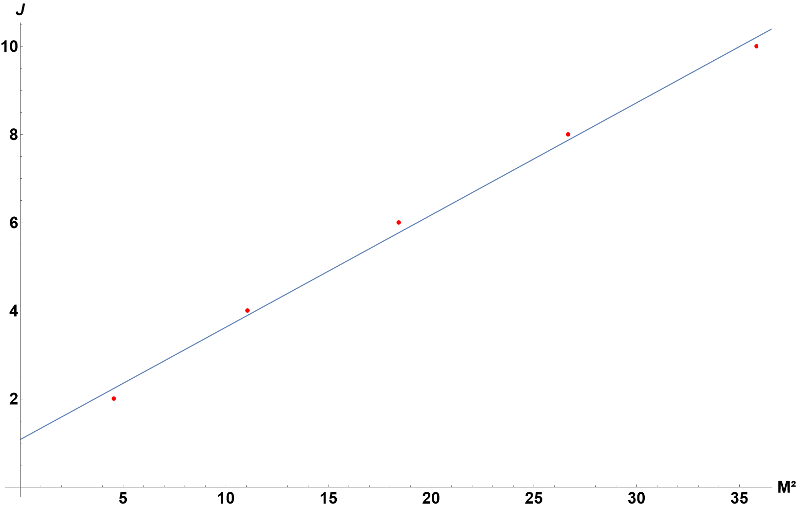
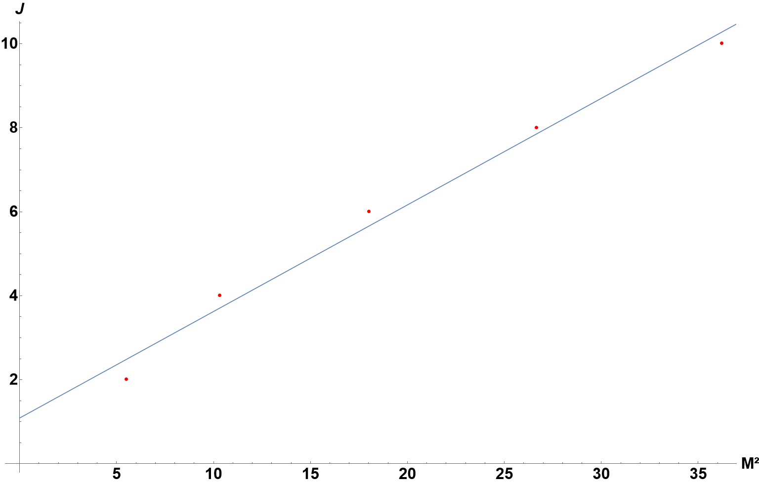
Figure 1: Plots of $J\times M^{2}$ with masses expressed in GeV and $J=2$ to $10$ in the anomalous models HW_log1 (Left panel) defined by Eq. (15), and HW_log2 (Right panel) Eq. (16). The dots represent the glueball masses shown in Table 2. Both straight lines correspond to linear fits matching the pomeron trajectory (13).

Another possible fit of the HW model with logarithm anomalous dimensions is to minimize directly the errors of the glueball masses with respect to lattice data and then look up for the resulting Regge trajectory. We consider this case with the state $0^{++}$ with canonical dimension $\Delta=4$ and for higher spins from $J=S=2$ to 10 with anomalous dimension given by Eq. (14). Applying this procedure one finds the coefficients $a=2.78$ and $b=2.18$, which means

$$\Delta_{\rm log3}=S+2.78\ln{(S)}+2.18,$$ (17)

obtaining exactly the lattice masses for the $2^{++}$ and $4^{++}$ states besides the $0^{++}$. For the state $6^{++}$, we find $M_{6^{++}}=4.88$ GeV which is $9\%$ higher than the lattice result. So, this model produces masses with lowest total relative error with respect to lattice outputs when compared with the logarithm anomalous HW models discussed above. However, within this model the fit of the pomeron trajectory produced by the states $2^{++}$, $4^{++}$, $6^{++}$, $8^{++}$, and $10^{++}$ is given by $S=0.20M^{2}+1.02$.

III.2 Approximate expressions for the anomalous dimensions

The conformal dimension for high spins from gauge/string duality discussed in the previous section was developed to describe an ideal situation where the four dimensional field theory is conformal. Since this is not the case of strong interactions that lead to the Regge trajectory of the soft pomeron and to the lattice glueball masses, it is interesting to investigate some approximate expressions for this quantity since we are studying a phenomenological model, and analyse whether these expressions give better results compared with experimental and lattice data.

Here, we start with the identity

$$\ln x=2\operatorname{arcsinh}\left[\frac{1}{2}\left(\sqrt{x}-\frac{1}{\sqrt{x}}\right)\right]\,,$$ (18)

which can be expanded for small $x$ as

$$\ln x = \sqrt{x}-\frac{1}{\sqrt{x}}-\frac{1}{24}\left(\sqrt{x}-\frac{1}{\sqrt{x}}\right)^{3}+\frac{3}{640}\left(\sqrt{x}-\frac{1}{\sqrt{x}}\right)^{5}+\cdots\,$$ (19)

$$= \sum_{k=0}^{\infty}\frac{(-1)^{k}}{2^{2k}(2k+1)k!}\left(\frac{1}{2}\right)_{k}\left(\sqrt{x}-\frac{1}{\sqrt{x}}\right)^{2k+1}\,,$$ (21)

where $(a)_{n}$ are the Pochhammer symbols. Using this expression we rewrite the effective dimension (14) as

$$\Delta = S+a\sum_{k=0}^{\infty}\frac{(-1)^{k}}{2^{2k}(2k+1)k!}\left(\frac{1}{2}\right)_{k}\left(\sqrt{S}-\frac{1}{\sqrt{S}}\right)^{2k+1}+b\,.$$ (22)

Now, truncating the series at some finite value of $k$ which means truncating at odd powers $2k+1$ of the difference $\sqrt{S}-1/\sqrt{S}$, we obtain approximate expressions for $\Delta$ from which we fit the soft pomeron trajectory and compare the obtained glueball masses with those from lattice calculations. Explicitly, we define this truncated effective dimension of high spin operators as

$$\Delta_{N} = S+a\sum_{k=0}^{N}\frac{(-1)^{k}}{2^{2k}(2k+1)k!}\left(\frac{1}{2}\right)_{k}\left(\sqrt{S}-\frac{1}{\sqrt{S}}\right)^{2k+1}+b\,.$$ (23)

Then, fixing the conformal dimension $\Delta=4$ for the $0^{++}$ state and taking Eq. (23) as the effective dimension for the states $2^{++}$ up to $10^{++}$ truncated at $N$ with $N=0,1,2,3$, we successfully match the soft pomeron trajectory, Eq. (13), with the same significant figures in all of these four cases. The corresponding glueball masses together with the associated relative errors with respect to the lattice data and the values of the anomalous dimensions for each state are presented in Table 3. Analysing these results, we see that the cases $N=0$ and $N=2$ present the smaller relative errors with respect to lattice output. We understand this behavior since the truncations at $N=0$ and $N=2$ contribute positively to the anomalous dimension (23) in contrast to $N=1$ and $N=3$, once they come from an alternate series. In particular, the plots corresponding to the masses found from the approximate anomalous effective dimension (23), truncated at $N=0$ and $N=1$ are presented in Figure 2.

Table 3: Masses of the $J^{++}$ glueball operators in GeV from $J=0$ to $J=10$, from the hard wall model Eq. (8) considering the approximate conformal dimension Eq. (22), truncating the series at $N=0,1,2,3$, with the corresponding relative errors with respect to lattice data, and the anomalous dimensions $\Delta_{\rm anom.}^{N}\equiv\Delta_{N}-(4+S)$ of the states in this model for each value of $N$. The mass of the $0^{++}$ is inserted as an input from lattice.

$J^{PC}$	$M_{N=0}$	$\delta_{N=0}$	$\Delta_{\rm anom.}^{N=0}$	$M_{N=1}$	$\delta_{N=1}$	$\Delta_{\rm anom.}^{N=1}$	$M_{N=2}$	$\delta_{N=2}$	$\Delta_{\rm anom.}^{N=2}$	$M_{N=3}$	$\delta_{N=3}$	$\Delta_{\rm anom.}^{N=3}$
$0^{++}$	$1.59$	$0\%$	$0.0$	$1.59$	$0\%$	$0.0$	$1.59$	$0\%$	$0.0$	$1.59$	$0\%$	$0.0$
$2^{++}$	$2.22$	$7.1\%$	$-0.36$	1.96	$18\%$	$-1.03$	2.27	$5.0\%$	$-0.21$	1.80	$25\%$	$-1.47$
$4^{++}$	$3.34$	$12\%$	$0.74$	3.39	$11\%$	$0.87$	3.35	$12\%$	$0.77$	3.41	$10\%$	$0.94$
$6^{++}$	$4.31$	$3.8\%$	$1.49$	4.41	1.6$\%$	$0.81$	4.28	$4.7\%$	$1.41$	4.56	$1.8\%$	$2.22$
$8^{++}$	5.20	-	$2.08$	5.25	-	$2.25$	5.17	-	$2.00$	5.40	-	$2.69$
$10^{++}$	6.05	-	$2.60$	5.98	-	$2.37$	6.08	-	$2.68$	5.87	-	$2.07$

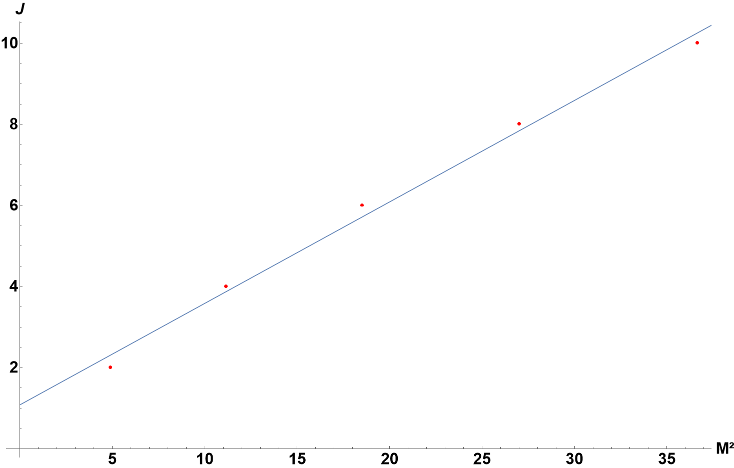
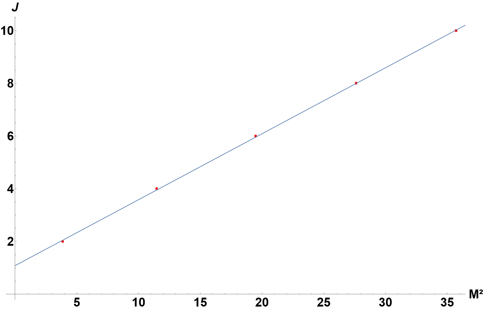
Figure 2: Plots of $J\times M^{2}$ with $M$ expressed in GeV and $J=2$ to $10$, using the approximate anomalous dimension Eq. (23), truncated at $N=0$ (left panel) with coefficients $a=1.38$ and $b=2.67$ and at $N=1$ (right panel) with $a=2.85$, $b=1.00$. The dots represent the glueball masses shown in Table 3 for $N=0$ and $N=1$, and the straight lines are the corresponding linear fits matching the pomeron trajectory (13).

III.3 Square root anomalous dimension

Here we consider another phenomenological for the anomalous dimension inspired by Eq. (23). Considering the truncation of this equation at $N=0$, and a further approximation we write the effective dimension for the high spin operators as

$$\Delta_{\rm SQRT}=S+a\sqrt{S}+b,$$ (24)

which represent square root anomalous dimensions. This approximation can be justified once we are taking the spins $S$ from 2 to 10 and the correction from the inverse square root is small in this range. Using this expression for the effective dimension of the glueball operators starting with $S=2$, and minimizing the resulting linear trajectory for the corresponding glueball masses, we find the coefficients $a=1.5$, $b=2.0$. The obtained glueball masses are listed in Table 4, together with the relative errors with respect to lattice data and the associated anomalous dimensions for each $J^{++}$ state. The resulting Regge trajectory, $J=0.25M^{2}+0.89$, is poorer than the corresponding ones from Eq. (23) shown in Table 3 which match with the same significant figures the pomeron trajectory Eq. (13). However it is remarkable that this simple model produces masses from Eq. (24) that have smaller relative errors with respect to lattice data, in comparison with the results of Tables 2 and 3.

Table 4: Masses of the $J^{++}$ glueball operators in GeV from $J=0$ to $J=10$, from the hard wall model Eq. (8) considering the square root anomalous dimension $\Delta_{\rm SQRT}$ from Eq. (24), with the corresponding relative errors $\delta_{\rm SQRT}$ with respect to lattice data, and the anomalous dimensions $\Delta_{\rm anom.}^{\rm SQRT}\equiv\Delta_{\rm SQRT}-(4+S)$ of the states $J^{++}$ in this case.

$J^{PC}$	$M_{\rm SQRT}$	$\delta_{\rm SQRT}$	$\Delta_{\rm anom.}^{\rm SQRT}$
$0^{++}$	$1.59$	$0\%$	$0.0$
$2^{++}$	2.40	$0.4\%$	$0.12$
$4^{++}$	3.44	$9.5\%$	$1.00$
$6^{++}$	4.38	$2.2\%$	$1.67$
$8^{++}$	5.27	-	$2.24$
$10^{++}$	6.12	-	$2.74$

IV Linear Hard Wall Model

Based on the arguments about the zeros of the Bessel functions presented at the end of Section II (just before Subsection II.1), we expect that a relation such as $\Delta\approx\sqrt{S}$ would asymptotically lead to a linear $J\times M^{2}$ graph. Moreover, the results of the previous section, also show the relevance of square root anomalous dimensions.

However, all the previous models discussed in this work do not lead to linear Regge trajectories if we extend the range to spins much higher than 10. To obtain such a trajectory we need to write the effective dimension of the high spin operators as a function of $\sqrt{S}$ without the linear term $S$. It is not difficult to see that the linear part on the spin $S$ of the discussed conformal dimensions always imply a quadratic behavior for the Regge trajectory. Then, from a phenomenological point of view, we consider an effective dimension for high spin $S$ operators, given by

$$\Delta_{\rm LHW}=a\sqrt{S}+b.$$ (25)

In order to check the possible linearity of this proposal we need to go to very high spin values. The best fit for the soft pomeron trajectory from $S=2$ to $100$ with this expression is obtained for $a=6.20$, and $b=-3.35$, such that the effective dimension reads

$$\Delta_{\rm LHW}=6.20\sqrt{S}-3.35.$$ (26)

The resulting trajectory is plotted in Figure 3, and is in perfect agreement with the experimental soft pomeron trajectory (13). The masses for glueballs obtained from this effective dimension are shown in Table 5, together with the relative errors with respect to lattice data, and the corresponding anomalous dimensions of the states $J^{++}$.

Table 5: Masses of the $J^{++}$ glueball operators in GeV from $J=0$ to $J=10$ within the linear hard wall (LHW) model, Eqs. (8) and (26). The mass of the $0^{++}$ state is inserted as an input from lattice. We also show the relative errors $\delta_{\rm LHW}$ compared with lattice data, and the anomalous dimensions $\Delta_{\rm anom.}^{\rm LHW}\equiv\Delta_{\rm anom.}-(4+S)$ of the glueball operators $J^{++}$ in this model.

$J^{PC}$	LHW	$\delta_{\rm LHW}$	$\Delta_{\rm anom.}^{\rm LHW}$
$0^{++}$	$1.59$	$0\%$	$0.0$
$2^{++}$	$2.14$	$10.46\%$	$-0.58$
$4^{++}$	$3.46$	$8.95\%$	$1.05$
$6^{++}$	$4.44$	$0.89\%$	$1.84$
$8^{++}$	$5.96$	-	$2.19$
$10^{++}$	$6.59$	-	$2.26$

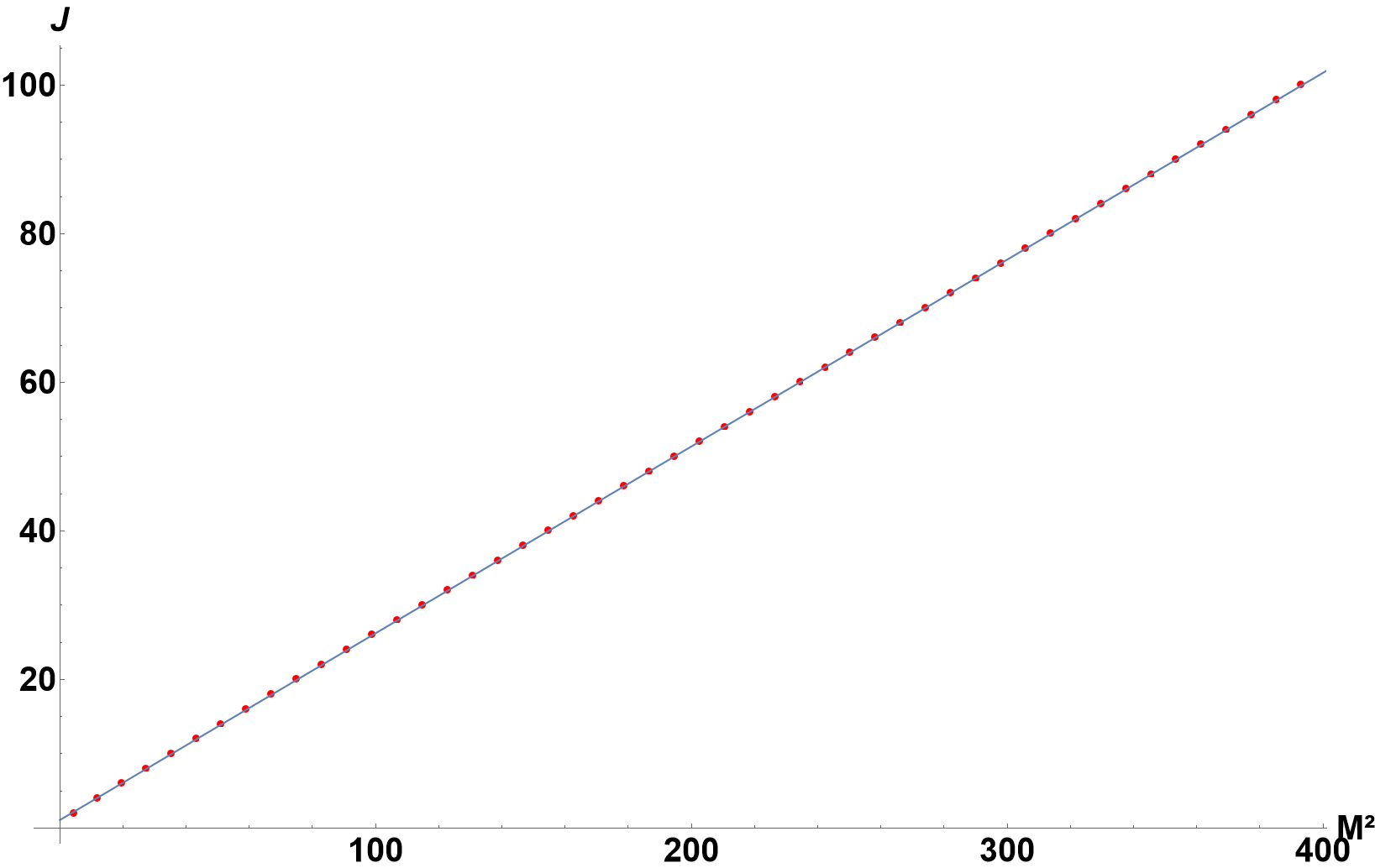
Figure 3: Regge trajectory $J\times M^{2}$ for the linear HW model defined by Eqs. (8) and (26), from $J=2$ to $J=100$. The dots represent the glueball masses obtained from this equation and their values corresponding to states from $J=2$ to $J=10$ are shown in Table 5. The straight line is the corresponding linear fit in the range from $J=2$ to $J=100$, matching the pomeron trajectory Eq. (13).

Comparing the above results with the ones from Eq. (23), one may wonder whether a contribution of the inverse of the square root of $S$ would spoil the linearity just found. Actually, considering a model with effective dimension given by $\Delta_{N=0}=a(\sqrt{S}-{1}/{\sqrt{S}})+b$, it is possible to obtain an asymptotic linear Regge trajectory. Fitting the states from $J=2$ to $J=10$ with the soft pomeron Regge trajectory Eq. (13) we match with the same significant figures, with coefficients $a=5.40$ and $b=0.86$. The masses obtained for these states are $\{1.85,3.42,4.44,5.25,5.93\}$ GeV, with relative errors $\{22.6,10.0,0.89\}\%$ with respect to lattice data. So, the result from Eq. (26) is better. The other powers $N=1,2,3$ of the difference $\sqrt{S}-{1}/{\sqrt{S}}$ discussed in the previous section, do not lead to asymptotic linear trajectories when high spins are considered, since they grow with $S^{(2N+1)/2}$.

V Conclusions

In this work we propose an anomalous hard wall model, starting from the original HW modifying its conformal dimension for high spins $S$ introducing anomalous dimensions according to results from a semi-classical limit of gauge/string dualities. According to these results for low spins the dimension of the spin operators are conformal $(\Delta=S+4)$ as in the original HW model. For high spins, these operators acquire anomalous dimensions in the form of a logarithm of $S$. Disregarding a complicated intermediate non-perturbative spin dependence, we take these results as a prescription to build up anomalous HW models. In general, to compare these models with experimental and lattice data, we adopt the strategy of first fitting the pomeron trajectory and then look up for the glueball masses to be compared with lattice results.

In Section III.1, we use these logarithm anomalous dimensions and propose three HW models, HW_log1, HW_log2 and HW_log3. In the first two models we follow the procedure of fitting the pomeron trajectory and then compare the glueball mass output with lattice data. In the third we reverse this approach and fit the lattice masses and then compare the resulting Regge trajectory with that of the pomeron. The first two models fit the pomeron trajectory Eq. (13) with the same significant figures, while the third give $S=0.20M^{2}+1.02$. Regarding glueball masses the three have total relative errors smaller than the original HW, and in particular the third model has the lowest total relative error with respect to lattice data.

In Section III.2 we discuss approximations to the logarithm anomalous dimensions in the form of an infinite series of odd powers of $(\sqrt{S}-1/\sqrt{S})^{2N+1}$ which are truncated at $N=0,1,2,3$. In these four cases they fit the pomeron trajectory Eq. (13) with the same significant figures. Regarding the glueball masses preditions when compared with lattice data, the cases with $N=0$ and $N=2$ present smaller relative errors than the cases $N=1$ and $N=3$. In particular, for $N=0,1,2$ the total relative errors are smaller than that of the original HW, while for $N=3$ they are of the same order of magnitude.

Inspired by the above results, in Section III.3 we discuss a HW model with square root anomalous dimensions. This model give as an output the Regge trajectory $J=0.25M^{2}+0.89$, which does not fit exactly the pomeron trajectory. On the other side, with respect to the glueball masses in comparison with lattice data, this model present the smaller total error than the models given by Eq. (23) and the logarithm models HW_log1 and HW_log2.

In Section IV, we propose a linear hard wall model leading to linear Regge trajectories even for very high spins. The original HW model is well known for producing non-linear Regge trajectories. The main modification introduced in the linear model is that we take $\Delta=a\sqrt{S}+b$ without the linear term $S$ present in all anomalous models discussed above and in the original HW model. The obtained Regge trajectory fits that of the soft pomeron Eq. (13) with the same significant figures, and the glueball masses compare well to lattice data with total relative error of the order of some above anomalous HW models, better than the original HW model.

In conclusion, these anomalous HW models represent a significant improvement with respect to the original HW model. This procedure of modifying the HW model with the inclusion of anomalous dimensions might be useful for other hadrons as mesons and baryons. This is presently under investigation.

References

- (1) F. Gross, E. Klempt, S. J. Brodsky, A. J. Buras, V. D. Burkert, G. Heinrich, K. Jakobs, C. A. Meyer, K. Orginos and M. Strickland, et al. “50 Years of Quantum Chromodynamics,” [arXiv:2212.11107 [hep-ph]].
- (2) O. Aharony, S. S. Gubser, J. M. Maldacena, H. Ooguri and Y. Oz, “Large N field theories, string theory and gravity,” Phys. Rept. 323, 183-386 (2000) doi:10.1016/S0370-1573(99)00083-6 [arXiv:hep-th/9905111 [hep-th]].
- (3) J. Polchinski and M. J. Strassler, “Hard scattering and gauge / string duality,” Phys. Rev. Lett. 88, 031601 (2002) doi:10.1103/PhysRevLett.88.031601 [arXiv:hep-th/0109174 [hep-th]].
- (4) J. Polchinski and M. J. Strassler, “Deep inelastic scattering and gauge / string duality,” JHEP 05, 012 (2003) doi:10.1088/1126-6708/2003/05/012 [arXiv:hep-th/0209211 [hep-th]].
- (5) S. S. Gubser, I. R. Klebanov and A. M. Polyakov, “A Semiclassical limit of the gauge / string correspondence,” Nucl. Phys. B 636, 99-114 (2002) doi:10.1016/S0550-3213(02)00373-5 [arXiv:hep-th/0204051 [hep-th]].
- (6) C. Csaki, H. Ooguri, Y. Oz and J. Terning, “Glueball mass spectrum from supergravity,” JHEP 01, 017 (1999) doi:10.1088/1126-6708/1999/01/017 [arXiv:hep-th/9806021 [hep-th]].
- (7) R. de Mello Koch, A. Jevicki, M. Mihailescu and J. P. Nunes, “Evaluation of glueball masses from supergravity,” Phys. Rev. D 58, 105009 (1998) doi:10.1103/PhysRevD.58.105009 [arXiv:hep-th/9806125 [hep-th]].
- (8) A. Hashimoto and Y. Oz, “Aspects of QCD dynamics from string theory,” Nucl. Phys. B 548, 167-179 (1999) doi:10.1016/S0550-3213(99)00120-0 [arXiv:hep-th/9809106 [hep-th]].
- (9) C. Csaki, Y. Oz, J. Russo and J. Terning, “Large N QCD from rotating branes,” Phys. Rev. D 59, 065012 (1999) doi:10.1103/PhysRevD.59.065012 [arXiv:hep-th/9810186 [hep-th]].
- (10) J. A. Minahan, “Glueball mass spectra and other issues for supergravity duals of QCD models,” JHEP 01, 020 (1999) doi:10.1088/1126-6708/1999/01/020 [arXiv:hep-th/9811156 [hep-th]].
- (11) R. C. Brower, S. D. Mathur and C. I. Tan, “Glueball spectrum for QCD from AdS supergravity duality,” Nucl. Phys. B 587, 249-276 (2000) doi:10.1016/S0550-3213(00)00435-1 [arXiv:hep-th/0003115 [hep-th]].
- (12) E. Caceres and R. Hernandez, “Glueball masses for the deformed conifold theory,” Phys. Lett. B 504, 64-70 (2001) doi:10.1016/S0370-2693(01)00278-7 [arXiv:hep-th/0011204 [hep-th]].
- (13) H. Boschi-Filho and N. R. F. Braga, “Gauge / string duality and scalar glueball mass ratios,” JHEP 05, 009 (2003) doi:10.1088/1126-6708/2003/05/009 [arXiv:hep-th/0212207 [hep-th]].
- (14) H. Boschi-Filho and N. R. F. Braga, “QCD / string holographic mapping and glueball mass spectrum,” Eur. Phys. J. C 32, 529-533 (2004) doi:10.1140/epjc/s2003-01526-4 [arXiv:hep-th/0209080 [hep-th]].
- (15) R. Apreda, D. E. Crooks, N. J. Evans and M. Petrini, “Confinement, glueballs and strings from deformed AdS,” JHEP 05, 065 (2004) doi:10.1088/1126-6708/2004/05/065 [arXiv:hep-th/0308006 [hep-th]].
- (16) X. Amador and E. Caceres, “Spin two glueball mass and glueball regge trajectory from supergravity,” JHEP 11, 022 (2004) doi:10.1088/1126-6708/2004/11/022 [arXiv:hep-th/0402061 [hep-th]].
- (17) N. Evans, J. P. Shock and T. Waterson, “Towards a perfect QCD gravity dual,” Phys. Lett. B 622, 165-171 (2005) doi:10.1016/j.physletb.2005.07.014 [arXiv:hep-th/0505250 [hep-th]].
- (18) E. Caceres and C. Nunez, “Glueballs of super Yang-Mills from wrapped branes,” JHEP 09, 027 (2005) doi:10.1088/1126-6708/2005/09/027 [arXiv:hep-th/0506051 [hep-th]].
- (19) H. Boschi-Filho, N. R. F. Braga and H. L. Carrion, “Glueball Regge trajectories from gauge/string duality and the Pomeron,” Phys. Rev. D 73, 047901 (2006) doi:10.1103/PhysRevD.73.047901 [arXiv:hep-th/0507063 [hep-th]].
- (20) E. Folco Capossoli and H. Boschi-Filho, “Odd spin glueball masses and the Odderon Regge trajectories from the holographic hardwall model,” Phys. Rev. D 88, no.2, 026010 (2013) doi:10.1103/PhysRevD.88.026010 [arXiv:1301.4457 [hep-th]].
- (21) T. Sakai and S. Sugimoto, “Low energy hadron physics in holographic QCD,” Prog. Theor. Phys. 113, 843-882 (2005) doi:10.1143/PTP.113.843 [arXiv:hep-th/0412141 [hep-th]].
- (22) T. Sakai and S. Sugimoto, “More on a holographic dual of QCD,” Prog. Theor. Phys. 114, 1083-1118 (2005) doi:10.1143/PTP.114.1083 [arXiv:hep-th/0507073 [hep-th]].
- (23) G. F. de Teramond and S. J. Brodsky, “Hadronic spectrum of a holographic dual of QCD,” Phys. Rev. Lett. 94, 201601 (2005) doi:10.1103/PhysRevLett.94.201601 [arXiv:hep-th/0501022 [hep-th]].
- (24) K. Ghoroku, N. Maru, M. Tachibana and M. Yahiro, “Holographic model for hadrons in deformed AdS(5) background,” Phys. Lett. B 633, 602-606 (2006) doi:10.1016/j.physletb.2005.12.004 [arXiv:hep-ph/0510334 [hep-ph]].
- (25) J. Erlich, E. Katz, D. T. Son and M. A. Stephanov, “QCD and a holographic model of hadrons,” Phys. Rev. Lett. 95, 261602 (2005) doi:10.1103/PhysRevLett.95.261602 [arXiv:hep-ph/0501128 [hep-ph]].
- (26) L. Da Rold and A. Pomarol, “Chiral symmetry breaking from five dimensional spaces,” Nucl. Phys. B 721, 79-97 (2005) doi:10.1016/j.nuclphysb.2005.05.009 [arXiv:hep-ph/0501218 [hep-ph]].
- (27) A. Karch, E. Katz, D. T. Son and M. A. Stephanov, “Linear confinement and AdS/QCD,” Phys. Rev. D 74, 015005 (2006) doi:10.1103/PhysRevD.74.015005 [arXiv:hep-ph/0602229 [hep-ph]].
- (28) S. J. Brodsky and G. F. de Teramond, “Hadronic spectra and light-front wavefunctions in holographic QCD,” Phys. Rev. Lett. 96, 201601 (2006) doi:10.1103/PhysRevLett.96.201601 [arXiv:hep-ph/0602252 [hep-ph]].
- (29) H. Hata, T. Sakai, S. Sugimoto and S. Yamato, “Baryons from instantons in holographic QCD,” Prog. Theor. Phys. 117, 1157 (2007) doi:10.1143/PTP.117.1157 [arXiv:hep-th/0701280 [hep-th]].
- (30) H. Forkel, M. Beyer and T. Frederico, “Linear square-mass trajectories of radially and orbitally excited hadrons in holographic QCD,” JHEP 07, 077 (2007) doi:10.1088/1126-6708/2007/07/077 [arXiv:0705.1857 [hep-ph]].
- (31) U. Gursoy and E. Kiritsis, “Exploring improved holographic theories for QCD: Part I,” JHEP 02, 032 (2008) doi:10.1088/1126-6708/2008/02/032 [arXiv:0707.1324 [hep-th]].
- (32) U. Gursoy, E. Kiritsis and F. Nitti, “Exploring improved holographic theories for QCD: Part II,” JHEP 02, 019 (2008) doi:10.1088/1126-6708/2008/02/019 [arXiv:0707.1349 [hep-th]].
- (33) J. Erdmenger, N. Evans, I. Kirsch and E. Threlfall, “Mesons in Gauge/Gravity Duals - A Review,” Eur. Phys. J. A 35, 81-133 (2008) doi:10.1140/epja/i2007-10540-1 [arXiv:0711.4467 [hep-th]].
- (34) A. Vega and I. Schmidt, “Scalar hadrons in AdS(5) x S**5,” Phys. Rev. D 78, 017703 (2008) doi:10.1103/PhysRevD.78.017703 [arXiv:0806.2267 [hep-ph]].
- (35) W. de Paula, T. Frederico, H. Forkel and M. Beyer, “Dynamical AdS/QCD with area-law confinement and linear Regge trajectories,” Phys. Rev. D 79, 075019 (2009) doi:10.1103/PhysRevD.79.075019 [arXiv:0806.3830 [hep-ph]].
- (36) Z. Abidin and C. E. Carlson, “Nucleon electromagnetic and gravitational form factors from holography,” Phys. Rev. D 79, 115003 (2009) doi:10.1103/PhysRevD.79.115003 [arXiv:0903.4818 [hep-ph]].
- (37) T. Gutsche, V. E. Lyubovitskij, I. Schmidt and A. Vega, “Dilaton in a soft-wall holographic approach to mesons and baryons,” Phys. Rev. D 85, 076003 (2012) doi:10.1103/PhysRevD.85.076003 [arXiv:1108.0346 [hep-ph]].
- (38) D. Li, M. Huang and Q. S. Yan, “A dynamical soft-wall holographic QCD model for chiral symmetry breaking and linear confinement,” Eur. Phys. J. C 73, 2615 (2013) doi:10.1140/epjc/s10052-013-2615-3 [arXiv:1206.2824 [hep-th]].
- (39) S. J. Brodsky, G. F. de Teramond, H. G. Dosch and J. Erlich, “Light-Front Holographic QCD and Emerging Confinement,” Phys. Rept. 584, 1-105 (2015) doi:10.1016/j.physrep.2015.05.001 [arXiv:1407.8131 [hep-ph]].
- (40) J. Sonnenschein, “Holography Inspired Stringy Hadrons,” Prog. Part. Nucl. Phys. 92, 1-49 (2017) doi:10.1016/j.ppnp.2016.06.005 [arXiv:1602.00704 [hep-th]].
- (41) E. Folco Capossoli, M. A. Martín Contreras, D. Li, A. Vega and H. Boschi-Filho, “Hadronic spectra from deformed AdS backgrounds,” Chin. Phys. C 44, no.6, 064104 (2020) doi:10.1088/1674-1137/44/6/064104 [arXiv:1903.06269 [hep-ph]].
- (42) S. S. Afonin, “Towards reconciling the holographic and lattice descriptions of radially excited hadrons,” Eur. Phys. J. C 80, no.8, 723 (2020) doi:10.1140/epjc/s10052-020-8306-y [arXiv:2008.05610 [hep-ph]].
- (43) M. Rinaldi and V. Vento, “Meson and glueball spectroscopy within the graviton soft wall model,” Phys. Rev. D 104, no.3, 034016 (2021) doi:10.1103/PhysRevD.104.034016 [arXiv:2101.02616 [hep-ph]].
- (44) H. R. Grigoryan and A. V. Radyushkin, “Form Factors and Wave Functions of Vector Mesons in Holographic QCD,” Phys. Lett. B 650, 421-427 (2007) doi:10.1016/j.physletb.2007.05.044 [arXiv:hep-ph/0703069 [hep-ph]].
- (45) K. A. Mamo and I. Zahed, “Neutrino-nucleon DIS from holographic QCD: PDFs of sea and valence quarks, form factors, and structure functions of the proton,” Phys. Rev. D 104, no.6, 066010 (2021) doi:10.1103/PhysRevD.104.066010 [arXiv:2102.00608 [hep-ph]].
- (46) P. V. Landshoff, “Pomerons,”, published in “Elastic and Difractive Scattering” Proceedings, Ed. V. Kundrat and P. Zavada, 2002, arXiv:hep-ph/0108156.
- (47) H. B. Meyer and M. J. Teper, “Glueball Regge trajectories and the pomeron: A Lattice study,” Phys. Lett. B 605, 344-354 (2005) doi:10.1016/j.physletb.2004.11.036 [arXiv:hep-ph/0409183 [hep-ph]].
- (48) V. S. Fadin and L. N. Lipatov, “BFKL pomeron in the next-to-leading approximation,” Phys. Lett. B 429, 127-134 (1998) doi:10.1016/S0370-2693(98)00473-0 [arXiv:hep-ph/9802290 [hep-ph]].
- (49) M. J. Teper, “Physics from the lattice: Glueballs in QCD: Topology: SU(N) for all N,” [arXiv:hep-lat/9711011 [hep-lat]].
- (50) C. J. Morningstar and M. J. Peardon, “Efficient glueball simulations on anisotropic lattices,” Phys. Rev. D 56, 4043-4061 (1997) doi:10.1103/PhysRevD.56.4043 [arXiv:hep-lat/9704011 [hep-lat]].
- (51) C. J. Morningstar and M. J. Peardon, “The Glueball spectrum from an anisotropic lattice study,” Phys. Rev. D 60, 034509 (1999) doi:10.1103/PhysRevD.60.034509 [arXiv:hep-lat/9901004 [hep-lat]].
- (52) P. Lebiedowicz, O. Nachtmann and A. Szczurek, “Central exclusive diffractive production of a single photon in high-energy proton-proton collisions within the tensor-Pomeron approach,” Phys. Rev. D 107, no.7, 074014 (2023) doi:10.1103/PhysRevD.107.074014 [arXiv:2302.07192 [hep-ph]].