Frequency conditions for the global stability of nonlinear delay equations with several equilibria

Abstract.

In our adjacent work, we developed a spectral comparison principle for compound cocycles generated by delay equations. It allows to derive frequency conditions (inequalities) for the uniform exponential stability of such cocycles by means of their comparison with stationary problems. Such inequalities are hard to verify analytically, and in this work we develop approximation schemes to verify some of the arising frequency inequalities. Besides some general results, we mainly stick to the case of scalar equations. By means of the Suarez-Schopf delayed oscillator and the Mackey-Glass equations, we demonstrate applications of the theory to reveal regions in the space of parameters where the absence of closed invariant contours can be guaranteed. Since our conditions are robust, so close systems also satisfy them, we expect them to actually imply the global stability, as in known finite-dimensional results utilizing variants of the Closing Lemma which is still awaiting developments in infinite dimensions.

1. Introduction

1.1. Historical perspective: generalized Bendixson criterion and global stability problems

In the seminal paper [23] R.A. Smith presented a generalization of the Bendixson criterion for ordinary differential equations (ODEs) in $\mathbb{R}^{n}$. His abstract conditions were concerned with a continuous mapping $F$ of a bounded simple connected domain $\mathcal{D}$ in $\mathbb{R}^{n}$ such that $F(\mathcal{D})$ lies in a compact subset of $\mathcal{D}$. Then he proved that there are no closed invariant contours on which $F$ is bijective provided that the Hausdorff dimension of the maximal compact invariant subset $\mathcal{A}$ (attractor) is strictly less than $2$.

In applications to ODEs, $F$ is given by the time-$t$ mapping $\varphi^{t}$ of the semiflow $\varphi$ generated by an ODE and $\overline{\mathcal{D}}$ (the closure of $\mathcal{D}$ in $\mathbb{R}^{n}$) is a positively invariant w.r.t. $\varphi$ closed bounded region such that $\mathcal{A}:=\bigcap_{t\geq 0}\varphi^{t}(\overline{\mathcal{D}})$ is a compact subset of $\mathcal{D}$. In this case from the Liouville trace formula in [23] it was derived the condition

(1.1) $$\alpha_{1}(x)+\alpha_{2}(x)<0\text{ for any }x\in\overline{\mathcal{D}},$$

where $\alpha_{1}(x)$ and $\alpha_{2}(x)$ are the first and second largest eigenvalues of the additively symmetrized Jacobian matrix of the vector field at $x$. This condition guarantees the contraction of areas under the action of the differential $d_{q}\varphi^{t}$ of $\varphi^{t}$ as $t\to+\infty$ uniformly in $q\in\mathcal{A}$. This implies that the Hausdorff (or even fractal) dimension of $\mathcal{A}$ is strictly less than $2$ (see V.V. Cheyzhov and A.A. Ilyin [10]; N.V. Kuznetsov and V. Reitmann [13]; R. Temam [25]) and, consequently, the abstract Bendixson criterion can be applied. In [23], it was also noted that (1.1) is a robust condition, i.e. $C^{1}$-close systems also satisfy it. This allowed R.A. Smith to utilize the Improved Closing Lemma of C.C. Pugh and deduce from (1.1) that any nonwandering point must be an equilibrium and, moreover, any trajectory in $\mathcal{D}$ must necessarily converge to an equilibrium.

Later, condition (1.1) was sharped by M. Li and J.S. Muldowney [17, 19] with the aid of compound matrices and Lozinskii (logarithmic) norms. They also widely extended geometric ideas of Smith to semiflows in Banach spaces [18] and, in particular, established a generalized Bendixson criterion for such semiflows.

Moreover, G.A. Leonov and V.A. Boichenko [16] gave another sharper conditions with the aid of Lyapunov-like functions. Now this approach is known as the Leonov method (see N.V. Kuznetsov [15]). In the monograph of N.V. Kuznetsov and V. Reitmann [13] such an approach is combined with logarithmic norms.

In fact, all the mentioned results are implicitly concerned with showing that

(1.2) $$\lambda_{1}(\Xi)+\lambda_{2}(\Xi)<0,$$

where $\lambda_{1}(\Xi)$ and $\lambda_{2}(\Xi)$ are the first and second largest uniform Lyapunov exponents of the linearization cocycle $\Xi$ of $\varphi$ in $\overline{\mathcal{D}}$, i.e we have $\Xi^{t}(q,\cdot):=d_{q}\varphi^{t}$ for $q\in\overline{D}$ and $t\geq 0$ in terms of Section 2.2. In the terminology of [2], (1.2) is obtained by computing the infinitesimal growth exponents for the $2$-nd compound cocycle in an adapted metric. Then the so-called maximization procedure (or the averaging procedure in the case of [17]) is applied to estimate the quantity $\lambda_{1}(\Xi)+\lambda_{2}(\Xi)$ from above.

Such a sum as $\lambda_{1}(\Xi)+\lambda_{2}(\Xi)$, being the largest Lyapunov exponent of the $2$-fold compound extension $\Xi_{2}$ of $\Xi$, is upper semicontinuous w.r.t. $\Xi$ under natural conditions. This is the robustness that is required to obtain the convergence criteria. Moreover, the supremum used to compute the value $\lambda_{1}(\Xi)+\lambda_{2}(\Xi)$ is achieved on the attractor $\mathcal{A}$ and, consequently, it is the same for any $\mathcal{D}$ enclosing the same attractor (see [2]).

In [2], it is shown (under some natural conditions) that one can always adapt the metric (not necessarily coercive) on the 2-fold exterior power such that the maximization procedure will produce quantities arbitrarily close to $\lambda_{1}(\Xi)+\lambda_{2}(\Xi)$. Thus, on the geometrical level, there are no “autonomous convergence theorems” (in plural, as it is used in [17]), but rather the only one abstract statement concerned with (1.2). Diversity arises in applications due to the use of particular metrics for specific problems in order to verify (1.2). Of course, for efficient applications this approach demands constructing adapted metrics.

From the perspective of the analysis of systems depending on parameters, it is convenient to call a semiflow globally stable if any of its trajectories tends to the stationary set (see N.V.Kuznetsov et al. [14]). This term covers multistable systems (which are more common) and emphasizes the global character of the problem. In the space of parameters, the boundary of global stability distinguishes the regions with simple and complex behavior.

From (1.2) we immediately see limitations of the method. Namely, the first $\lambda_{1}$ and second $\lambda_{2}$ (as the real part decreases) eigenvalues at any equilibrium from $\mathcal{D}$ must satisfy $\operatorname{Re}\lambda_{1}+\operatorname{Re}\lambda_{2}<0$. There are systems where the boundary of global stability is determined by local bifurcations of equilibria (usually, the Andronov-Hopf bifurcation). In this case the boundary is called trivial in the terminology of [14]. For such systems the criterion based on (1.2) has a prospect (with the use of adapted metrics) to reveal all the region of global stability provided that there are no saddles with $\operatorname{Re}\lambda_{1}+\operatorname{Re}\lambda_{2}\geq 0$, until the bifurcation occurs. However, there are systems where the boundary of global stability is determined by nonlocal bifurcations (such as the Lorenz system) and in this case the boundary is called hidden. For such systems, applications of analytical methods may be complicated. Looking ahead, we note that the Suarez-Schopf model (see Section 4.5) has a hidden boundary of global stability and the Mackey-Glass model (see Section 4.6) is conjectured to have a trivial boundary.

The above considerations can be illustrated by means of the Lorenz system for which the conditions given by R.A. Smith [23] were improved in [16]. Moreover, N.V. Kuznetsov et al. [14] derived an exact analytical formula for the Lyapunov dimension of the global attractor in the Lorenz system by developing the Leonov method. As a consequence, there is an analytical description of the region where (1.2) is satisfied and this is the maximum that can be achieved via the generalized Bendixson criterion.

1.2. Contribution of the present work

This paper is concerned with applications of the generalized Bendixson criterion developed by M.Y. Li and J.S. Muldowney [18] to delay equations in $\mathbb{R}^{n}$ by verifying (1.2) for the corresponding linearization cocycles. This problem is related to the problem of obtaining effective dimension estimates for such equations and it is rarely addressed in the known literature (see [2, 5] for discussions). To the best of our knowledge, the first satisfactory results in this direction were obtained in [2]. In particular, dimension estimates for the global attractor in the Mackey-Glass equations, which seem to be asymptotically sharp (i.e. up to a constant) as the delay value tends to infinity, are obtained therein. Although such estimates provide nontrivial regions where (1.2) holds, numerical analysis indicates much larger regions of global stability.

Here we follow the approach developed in our adjacent paper [3], where a spectral comparison principle for compound cocycles in Hilbert spaces generated by delay equations is established. This principle treats the compound cocycle as a nonautonomous perturbation of a $C_{0}$-semigroup and provides frequency conditions (inequalities) to guarantee that certain properties concerned with spectral dichotomies of the semigroup will be preserved under such a perturbation. Here the perturbation is described through the so-called quadratic constraints and the perturbation problem is posed in the context of an appropriate infinite-horizon quadratic regulator problem, which, in its turn, is resolved via the Frequency Theorem developed by us in [1] (see also [7]). In particular, the principle provides frequency conditions for the uniform exponential stability of compound cocycles. This is clearly related to the initial problem, since in terms of such cocycles (1.2) means that the $2$-nd compound cocycle is uniformly exponentially stable. On the geometric level, the frequency conditions guarantee the existence of an adapted metric given by a positive-definite quadratic functional on the exterior power (see Theorem 3.2). Although it is not necessarily coercive, its relation with the dynamics allows to obtain the required bound (see Corollary 3.2). We give a brief exposition of this theory in Section 3.

However, for the verification of arising frequency inequalities we need to compute resolvents of additive compound operators. In the case of delay equations, this reduces to solving a first-order PDE with boundary conditions involving both partial derivatives and delays. This prevents dealing with the problem in a purely analytical way.

In this paper, we are aimed to develop approximation schemes to verify frequency inequalities and consider implementations of such schemes for conducting reliable numerical experiments (see Section 4). Besides some abstract results, we mainly stick to the case of scalar equations. We give applications to the Suarez-Schopf delayed oscillator (see Section 4.5), which is a system with a hidden boundary of global stability (see [4]), and the Mackey-Glass equations (see Section 4.6), which is conjectured to be a system with a trivial boundary of global stability (see Conjecture 2). For these models, the developed machinery indicates more sharper regions of global stability than the purely analytical results from [5] and [2] (see the sections for more detailed discussions).

Note also that the frequency-domain approach to the uniform exponential stability of compound cocycles is potentially applicable to a range of problems, including, for example, parabolic or hyperbolic equations (possibly with delay). However, besides this and the adjacent [3] papers, we do not know such applications even in the case of ODEs. As to delay equations, here the general approach presented in [1] reveals specificity of such equations and leads to the discovery of their important analytical properties which we call structural Cauchy formulas. Such properties are related to the well-posedness of the infinite-horizon quadratic regulator problem. Although the analytical side of our approach constituted by [3] and [1] may seem complicated (especially for experimentalists), the approximation scheme Approximation scheme: statement-Approximation scheme: statement stated in Section 4.2 shall be accessible to a wide audience.

To the best of our knowledge, there is still no variant of the Closing Lemma which is appropriate for infinite dimensional problems and delay equations in particular. We hope that our research will stimulate developments in this direction. Since we lack of such a lemma, we are unable to prove that our conditions generally imply the global stability, but we believe in this because of their robustness. However, in the case of the Suarez-Schopf delayed oscillator, the problem can be avoided since the system belongs to the class of monotone feedback systems which satisfy the Poincaré-Bendixson trichotomy (see J. Mallet-Paret and G.R. Sell [22]). Moreover, for some delay equations one may construct finite-dimensional inertial manifolds (see [1, 6, 8]) and apply the usual Closing Lemma.

This paper is organized as follows. In Section 2 we introduce basic definitions. Namely, in Section 2.1 we briefly discuss tensor products of Hilbert spaces and compound operators on $m$-fold tensor products. In Section 2.2 we give definitions of semiflows and cocycles. In Section 3 we expound a part of the theory developed in [3] which is necessary to introduce frequency conditions for the uniform exponential stability of compound cocycles generated by delay equations (see Theorem 3.2). In Section 4 we develop approximation schemes to verify frequency inequalities (see Section 4.3 for the statement and Section 4.4 for a discussion) and give applications to the Suarez-Schopf delayed oscillator (see Section 4.5) and Mackey-Glass equations (see Section 4.6).

2. Preliminaries

2.1. Multiplicative and additive compound operators on tensor products of Hilbert spaces

Let us briefly discuss basic concepts concerned with tensor products of Hilbert spaces (see, for example, R. Temam [25]). Let $\mathbb{H}_{1}$ and $\mathbb{H}_{2}$ be two real or complex Hilbert spaces. By $\mathbb{H}_{1}\odot\mathbb{H}_{2}$ we denote the algebraic tensor product of $\mathbb{H}_{1}$ and $\mathbb{H}_{2}$. Recall that it is spanned by decomposable tensors $v_{1}\otimes v_{2}$, where $v_{1}\in\mathbb{H}_{1}$ and $v_{2}\in\mathbb{H}_{2}$, given by the equivalence class of the pair $(v_{1},v_{2})$ in the free vector space over the Cartesian product $\mathbb{H}_{1}\times\mathbb{H}_{2}$ factorized under bilinear equivalence relations. We endow $\mathbb{H}_{1}\odot\mathbb{H}_{2}$ with the inner product defined as

(2.1) $$(v_{1}\otimes v_{2},w_{1}\otimes w_{2}):=(v_{1},w_{1})\cdot(v_{2},w_{2})$$

for any $v_{1},w_{1}\in\mathbb{H}_{1}$ and $v_{2},w_{2}\in\mathbb{H}_{2}$. This formula indeed correctly defines an inner product in $\mathbb{H}_{1}\odot\mathbb{H}_{2}$ due to the universal property of algebraic tensor products. Now the tensor product $\mathbb{H}_{1}\otimes\mathbb{H}_{2}$ of $\mathbb{H}_{1}$ and $\mathbb{H}_{2}$ is defined as the completion of $\mathbb{H}_{1}\odot\mathbb{H}_{2}$ by the norm induced by (2.1).

For given Hilbert spaces $\mathbb{H}_{1},\mathbb{H}_{2},\mathbb{W}_{1}$ and $\mathbb{W}_{2}$ and bounded linear operators $L_{1}\in\mathcal{L}(\mathbb{H}_{1};\mathbb{W}_{1})$ and $L_{2}\in\mathcal{L}(\mathbb{H}_{2};\mathbb{W}_{2})$, there is a unique operator $L_{1}\otimes L_{2}\in\mathcal{L}(\mathbb{H}_{1}\otimes\mathbb{H}_{2};\mathbb{W}_{1}\otimes\mathbb{W}_{2})$ (called the tensor product of $L_{1}$ and $L_{2}$) such that

(2.2) $$(L_{1}\otimes L_{2})(v_{1}\otimes v_{2})=L_{1}v_{1}\otimes L_{2}v_{2}\text{ for any }v_{1}\in\mathbb{H}_{1},v_{2}\in\mathbb{H}_{2}.$$

It can be shown that $\|L_{1}\otimes L_{2}\|=\|L_{1}\|\cdot\|L_{2}\|$. Moreover, by definition, the tensor product of operators behaves well w.r.t. compositions of operators in the sense that $(BA)\otimes(DC)=(B\otimes D)(A\otimes C)$ for any bounded linear operators $A,B,C$ and $D$ defined on appropriate spaces.

For any triple $\mathbb{H}_{1},\mathbb{H}_{2}$ and $\mathbb{H}_{3}$ of Hilbert spaces we have that the tensor products $(\mathbb{H}_{1}\otimes\mathbb{H}_{2})\otimes\mathbb{H}_{3}$ and $\mathbb{H}_{1}\otimes(\mathbb{H}_{2}\otimes\mathbb{H}_{3})$ are naturally isometrically isomorphic and therefore denoted just by $\mathbb{H}_{1}\otimes\mathbb{H}_{2}\otimes\mathbb{H}_{3}$. This allows to carry the above constructions to any finite product $\mathbb{H}_{1}\otimes\ldots\otimes\mathbb{H}_{m}$ of Hilbert spaces.

For a given Hilbert space $\mathbb{H}$ and an integer $m>0$ we define the $m$-fold tensor product $\mathbb{H}^{\otimes m}$ of $\mathbb{H}$ as $\mathbb{H}^{\otimes m}:=\mathbb{H}\otimes\ldots\otimes\mathbb{H}$ ($m$ times). Then for any $L\in\mathcal{L}(\mathbb{H})$ we denote its $m$-fold product $L\otimes\ldots\otimes L\in\mathcal{L}(\mathbb{H}^{\otimes m})$ as $L^{\otimes m}$ and call it the $m$-fold multiplicative compound of $L$.

Let $\mathbb{S}_{m}$ be the symmetric group on $\{1,\ldots,m\}$. For each $\sigma\in\mathbb{S}_{m}$ let $S_{\sigma}\in\mathcal{L}(\mathbb{H}^{\otimes m})$ the transposition operator w.r.t. $\sigma$, i.e. for any $v_{1},\ldots,v_{m}\in\mathbb{H}$ we have

(2.3) $$S_{\sigma}(v_{1}\otimes\ldots\otimes v_{m})=v_{\sigma(1)}\otimes\ldots\otimes v_{\sigma(m)}.$$

Clearly, $S_{\sigma}$ is self-adjoint and $S^{-1}_{\sigma}=S_{\sigma^{-1}}$.

Let $\Pi^{\wedge}_{m}\in\mathcal{L}(\mathbb{H}^{\otimes m})$ be given as

(2.4) $$\Pi^{\wedge}_{m}:=\frac{1}{m!}\sum_{\sigma\in\mathbb{S}_{m}}(-1)^{\sigma}S_{\sigma}.$$

From the above properties of $S_{\sigma}$ it can be shown that $\Pi^{\wedge}_{m}$ is an orthogonal projector in $\mathbb{H}^{\otimes m}$. Let $\mathbb{H}^{\wedge m}$ be its image which is called the $m$-fold exterior product of $\mathbb{H}$. For any $v_{1},\ldots,v_{m}\in\mathbb{H}$ we put $v_{1}\wedge\ldots\wedge v_{m}:=\Pi^{\wedge}_{m}(v_{1}\otimes\ldots\otimes v_{m})$.

Clearly, for $L\in\mathcal{L}(\mathbb{H})$ the operator $L^{\otimes m}$ commutes with any $S_{\sigma}$ from (2.3) and, as a consequence, it commutes with $\Pi^{\wedge}_{m}$ from (2.4). Thus, $\mathbb{H}^{\wedge m}$ is invariant w.r.t. $L^{\otimes m}$. Let $L^{\wedge m}$ be the restriction of $L^{\otimes m}$ to $\mathbb{H}^{\wedge m}$ called the $m$-fold antisymmetric multiplicative compound of $L$. It will be sometimes convenient to say that $L^{\wedge m}$ is the $m$-fold multiplicative compound of $L$ in $\mathbb{H}^{\wedge m}$ and analogous terminology will be applied to related concepts given below for semigroups and cocycles. It is not hard to see that for any $v_{1},\ldots,v_{m}\in\mathbb{H}$ we have

(2.5) $$L^{\wedge m}(v_{1}\wedge\ldots\wedge v_{m})=Lv_{1}\wedge\ldots\wedge Lv_{m}.$$

Now suppose that $G$ is a $C_{0}$-semigroup in $\mathbb{H}$ (see K.-J. Engel and R. Nagel [11]) and let $G(t)\in\mathcal{L}(\mathbb{H})$ denote its time-$t$ mapping for $t\geq 0$. By $G^{\otimes m}$ (resp. $G^{\wedge m}$ ) we denote the semigroup called the $m$-fold multiplicative compound of $G$ in $\mathbb{H}^{\otimes m}$ (resp. $\mathbb{H}^{\wedge m}$) such that the time-$t$ mappings are given by $G^{\otimes m}(t):=(G(t))^{\otimes m}$ and $G^{\wedge m}(t):=(G(t))^{\wedge m}$ for $t\geq 0$. It can be shown (see Section 2 in [3]) that $G^{\otimes m}$ (resp. $G^{\wedge m}$) is a $C_{0}$-semigroup in $\mathbb{H}^{\otimes m}$ (resp. $\mathbb{H}^{\wedge m}$).

Suppose $A$ is the generator of a $C_{0}$-semigroup $G$ in $\mathbb{H}$. Let $A^{[\otimes m]}$ (resp. $A^{[\wedge m]}$) be the generator of $G^{\otimes m}$ (resp. $G^{\wedge m}$). Then $A^{[\otimes m]}$ (resp. $A^{[\wedge m]}$) is called the $m$-fold additive compound (resp. the $m$-fold antisymmetric additive compound) of $A$.

In the case $G$ is eventually norm continuous (resp. eventually compact), the semigroups $G^{\otimes m}$ and $G^{\wedge m}$ are also eventually norm continuous (resp. eventually compact) by Propositions 2.2 and 2.3 in [3]. In particular, the Spectral Mapping Theorem for Semigroups can be used to relate the spectrum of $A$ with the spectra of $A^{[\otimes m]}$ and $A^{[\wedge m]}$. In the case of eventually compact semigroups, which arise in the study of delay equations, we can relate eigenvalues and the corresponding spectral subspaces of $A$ and $A^{[\otimes m]}$ or $A^{[\wedge m]}$. In this work, the following property concerned with the spectral bound of $A^{[\wedge m]}$ is important.

Proposition 2.1.

Suppose that $G$ is eventually compact and let $\lambda_{1}(A)$, $\lambda_{2}(A)$, $\ldots$ be the eigenvalues of $A$ arranged by nonincreasing of real parts and according to their multiplicity. Then the spectral bound $s(A^{[\wedge m]})$ of $A^{[\wedge m]}$ is given by

(2.6) $$s(A^{[\wedge m]})=\sum_{j=1}^{m}\operatorname{Re}\lambda_{j}(A),$$

provided that $A$ has at least $m$ eigenvalues and $s(A^{[\wedge m]})=-\infty$ otherwise.

Proof.

Since $G$ is eventually compact, $G^{\wedge m}$ is also eventually compact by Proposition 2.2 in [3]. Thus, the spectrum of $A^{[\wedge m]}$ consists of eigenvalues having finite algebraic multiplicity (see Theorem 3.1, p. 329 in [11]) and for any $\nu\in\mathbb{R}$ the number of eigenvalues in each half-plane $\operatorname{Re}\lambda>\nu$ is finite (see Corollary 2.11, p. 258 in [11]). Consequently, the spectral bound $s(A^{[\wedge m]})$ of $A^{[\wedge m]}$ is given by the largest real part of its eigenvalues (either by $-\infty$ if the spectrum is empty).

By Theorem 2.2 in [3], the spectrum of $A^{[\otimes m]}$ consists of the sums

(2.7) $$\lambda_{0}:=\sum_{j=1}^{m}\lambda_{j},$$

where $\lambda_{j}$ is an eigenvalue of $A$ for any $j\in\{1,\ldots,m\}$, and for the corresponding to $\lambda_{0}$ spectral subspace $\mathbb{L}_{A^{[\otimes m]}}(\lambda_{0})$ of $A^{[\otimes m]}$ we have

(2.8) $$\mathbb{L}_{A^{[\otimes m]}}(\lambda_{0})=\bigoplus_{k=1}^{N}\bigotimes_{j=1}^{m}\mathbb{L}_{A}(\lambda^{k}_{j}),$$

where $N$ is the number of distinct $m$-tuples $(\lambda^{k}_{1},\ldots,\lambda^{k}_{m})$ enumerated by $k\in\{1,\ldots,N\}$ such that (2.7) holds with $\lambda_{j}=\lambda^{k}_{j}$ for any $j\in\{1,\ldots,m\}$ and $\mathbb{L}_{A}(\lambda^{k}_{j})$ is the spectral subspace of $A$ corresponding to $\lambda^{k}_{j}$.

Moreover, the spectrum of $A^{[\wedge m]}$ consists of exactly such $\lambda_{0}$ for which the projector $\Pi^{\wedge}_{m}$ from (2.4) does not vanish on $\mathbb{L}_{A^{[\otimes m]}}(\lambda_{0})$. In this case, $\Pi^{\wedge}_{m}\mathbb{L}_{A^{[\otimes m]}}(\lambda_{0})$ is the spectral subspace of $A^{[\wedge m]}$ corresponding to $\lambda_{0}$. Note that for this it is necessary and sufficient not to vanish on $\bigotimes_{j=1}^{m}\mathbb{L}_{A}(\lambda^{k}_{j})$ for some $k\in\{1,\ldots,N\}$.

Note that $\Pi^{\wedge}_{m}\bigotimes_{j=1}^{m}\mathbb{L}_{A}(\lambda^{k}_{j})\not=0$ if and only if each $\lambda^{k}_{j}$ does not occur in the $m$-tuple $(\lambda^{k}_{1},\ldots,\lambda^{k}_{m})$ more often than its algebraic multiplicity. Clearly, $\lambda_{0}=\sum_{j=1}^{m}\lambda_{j}(A)$ satisfies this condition and has the largest real part (either the spectrum is empty, if there are less than $m$ eigenvalues of $A$). The proof is finished. ∎

2.2. Semiflows and cocycles

Consider a time space $\mathbb{T}\in\{\mathbb{R}_{+},\mathbb{R}\}$, where $\mathbb{R}_{+}=[0,+\infty)$. A family of mappings $\vartheta^{t}(\cdot)\colon\mathcal{Q}\to\mathcal{Q}$, where $t\in\mathbb{T}$ and $\mathcal{Q}$ is a complete metric space, such that

(DS1):

For each $q\in\mathcal{Q}$ and $t,s\in\mathbb{T}$ we have $\vartheta^{t+s}(q)=\vartheta^{t}(\vartheta^{s}(q))$ and $\vartheta^{0}(q)=q$;

(DS2):

The mapping $\mathbb{T}\times\mathcal{Q}\ni(t,q)\mapsto\vartheta^{t}(q)$ is continuous,

is called a dynamical system on $\mathcal{Q}$. For brevity, we often use the notation $(\mathcal{Q},\vartheta)$ or simply $\vartheta$ to denote the dynamical system. In the case $\mathbb{T}=\mathbb{R}_{+}$ (resp. $\mathbb{T}=\mathbb{R}$) we call $\vartheta$ a semiflow (resp. a flow) on $\mathcal{Q}$.

Let a dynamical system $(\mathcal{Q},\vartheta)$ be fixed. For a given Banach space $\mathbb{E}$, a family of mappings $\psi^{t}(q,\cdot)\colon\mathbb{E}\to\mathbb{E}$, where $t\in\mathbb{R}_{+}$ and $q\in\mathcal{Q}$, is called a cocycle in $\mathbb{E}$ over $(\mathcal{Q},\vartheta)$ if

(CO1):

For all $v\in\mathbb{E}$, $q\in\mathcal{Q}$ and $t,s\in\mathbb{R}_{+}$ we have $\psi^{t+s}(q,v)=\psi^{t}(\vartheta^{s}(q),\psi^{s}(q,v))$ and $\psi^{0}(q,v)=v$;

(CO2):

The mapping $\mathbb{R}_{+}\times\mathcal{Q}\times\mathbb{E}\ni(q,t,v)\mapsto\psi^{t}(q,v)$ is continuous.

For brevity, we often denote such a cocycle by $\psi$. If each mapping $\psi^{t}(q,\cdot)$ belongs to the space $\mathcal{L}(\mathbb{E})$ of linear bounded operators in $\mathbb{E}$, we say that the cocycle is linear. Moreover, if it additionally satisfies

(UC1):

For any $t\in\mathbb{R}_{+}$ the mapping $\mathcal{Q}\ni q\mapsto\psi^{t}(q,\cdot)\in\mathcal{L}(\mathbb{E})$ is continuous in the operator norm;

(UC2):

The cocycle mappings are bounded uniformly in finite times, that is

(2.9) $$\sup_{t\in[0,1]}\sup_{q\in\mathcal{Q}}\|\psi^{t}(q,\cdot)\|_{\mathcal{L}(\mathbb{E})}<+\infty,$$

then $\psi$ is called a uniformly continuous linear cocycle. Note that for such cocycles Semiflows and cocycles is equivalent to that the operator $\psi^{t}(q,\cdot)$ depends continuously on $(t,q)$ in the strong operator topology.

In this paper, we deal with uniformly continuous linear cocycles in a Hilbert space $\mathbb{H}$. Let $\Xi$ be such a cocycle. For each integer $m>0$ we associate with $\Xi$ a cocycle $\Xi_{m}$ acting on the $m$-fold tensor product $\mathbb{H}^{\otimes m}$ of $\mathbb{H}$. For $\Xi_{m}$, each cocycle mapping $\Xi^{t}_{m}(q,\cdot)\in\mathcal{L}(\mathbb{H}^{\otimes m})$, where $t\geq 0$ and $q\in\mathcal{Q}$, is given by the $m$-fold multiplicative compound of $\Xi^{t}(q,\cdot)$ in $\mathbb{H}^{\otimes m}$. It can be shown that $\Xi_{m}$ is indeed a uniformly continuous cocycle and we call it the $m$-fold multiplicative compound of $\Xi$ in $\mathbb{H}^{\otimes m}$. Moreover, the same notation is used to denote the restriction of $\Xi_{m}$ to the $m$-fold exterior power $\mathbb{H}^{\wedge m}$ called the $m$-fold multiplicative compound of $\Xi$ in $\mathbb{H}^{\wedge m}$ or the $m$-fold antisymmetric multiplicative compound of $\Xi$. It will be clear from the context which cocycle is being referred to.

3. Exponential stability of compound cocycles generated by delay equations

3.1. Cocycles generated by nonautonomous delay equations

We are going to describe the class of delay equations to which our theory is applied. For this, let $\pi$ be a semiflow on a complete metric space $\mathcal{P}$. For some positive integers $r_{1}$ and $r_{2}$ we put $\mathbb{U}:=\mathbb{R}^{r_{1}}$ and $\mathbb{M}:=\mathbb{R}^{r_{2}}$, where the spaces are endowed with some (not necessarily Euclidean) inner products with the norms $|\cdot|_{\mathbb{U}}$ and $|\cdot|_{\mathbb{M}}$ respectively. We consider the class of nonautonomous delay equations in $\mathbb{R}^{n}$ over $(\mathcal{P},\pi)$ which are described over each $\wp\in\mathcal{P}$ as

(3.1) $$\dot{x}(t)=\widetilde{A}x_{t}+\widetilde{B}F^{\prime}(\pi^{t}(\wp))Cx_{t}.$$

Here $\tau>0$ is a fixed real number (delay); $x(\cdot)\colon[-\tau,T]\to\mathbb{R}^{n}$ for some $T>0$ and $x_{t}(\theta)=x(t+\theta)$ for $\theta\in[-\tau,0]$ denotes the $\tau$-history segment of $x(\cdot)$ at $t\in[0,T]$. Moreover, $\widetilde{A}\colon C([-\tau,0];\mathbb{R}^{n})\to\mathbb{R}^{n}$ and $C\colon C([-\tau,0];\mathbb{R}^{n})\to\mathbb{M}$ are bounded linear operators; $\widetilde{B}\colon\mathbb{U}\to\mathbb{R}^{n}$ is a linear operator and $F^{\prime}\colon\mathcal{P}\to\mathcal{L}(\mathbb{M};\mathbb{U})$ is a continuous mapping such that for some $\Lambda>0$ we have

(3.2) $$\|F^{\prime}(\wp)\|_{\mathcal{L}(\mathbb{M};\mathbb{U})}\leq\Lambda\text{ for all }\wp\in\mathcal{P}.$$

To discuss the well-posedness of (3.1), let us write it as an evolutionary equation in a proper Hilbert space. For this, consider the Hilbert space

(3.3) $$\mathbb{H}=L_{2}([-\tau,0];\mu;\mathbb{R}^{n}),$$

where the measure $\mu$ is given by the sum of the Lebesgue measure on $[-\tau,0]$ and the delta measure $\delta_{0}$ at $0$. For $\phi\in\mathbb{H}$ we write $R^{(1)}_{0}\phi=\phi(0)\in\mathbb{R}$ and $R^{(1)}_{1}\phi={\left.\kern-1.2pt\phi\vphantom{\big{|}}\right|_{(-\tau,0)}}\in L_{2}(-\tau,0;\mathbb{R}^{n})$. Here the upper index in the notation will be explained below.

With the operator $\widetilde{A}$ from (3.1) we associate the operator $A$ in $\mathbb{H}$ defined for $\phi\in\mathcal{D}(A)$ as

(3.4) $$R^{(1)}_{0}(A\phi)=\widetilde{A}R^{(1)}_{1}\phi\text{ and }R^{(1)}_{1}(A\phi)=\frac{d}{d\theta}R^{(1)}_{1}\phi,$$

where the domain $\mathcal{D}(A)$ of $A$ is given by the embedding of $W^{1,2}(-\tau,0;\mathbb{R}^{n})$ into $\mathbb{H}$ such that $\psi\in W^{1,2}(-\tau,0;\mathbb{R}^{n})$ is mapped into $\phi\in\mathbb{H}$ satisfying $R^{(1)}_{0}\phi=\psi(0)$ and $R^{(1)}_{1}\phi=\psi$. Since $W^{1,2}(-\tau,0;\mathbb{R}^{n})$ can be naturally continuously embedded into $C([-\tau,0];\mathbb{R}^{n})$, the definition is correct. Clearly, $A$ is a closed operator.

We also embed the space $\mathbb{E}=C([-\tau,0];\mathbb{R}^{n})$ into $\mathbb{H}$ by sending each $\psi\in\mathbb{E}$ into $\phi\in\mathbb{H}$ such that $R^{(1)}_{0}\phi=\psi(0)$ and $R^{(1)}_{1}\phi=\psi$. It will be convenient to identify the elements of $\mathbb{E}$ and their images in $\mathbb{H}$ under the embedding. In particular, we use the same notation for the operator $C$ from (3.1) and its composition with the embedding. Namely, we put $C\phi:=CR^{(1)}_{1}\phi=C\psi$ for $\phi\in\mathbb{H}$ and $\psi\in\mathbb{E}$ related by the just introduced embedding.

Now define a bounded linear operator $B\colon\mathbb{U}\to\mathbb{H}$ as $R^{(1)}_{0}B\eta=\widetilde{B}\eta$ and $R^{(1)}_{1}B\eta=0$ for $\eta\in\mathbb{U}$. Then (3.1) can be treated as an abstract evolution equation in $\mathbb{H}$ given by

(3.5) $$\dot{\xi}(t)=A\xi(t)+BF^{\prime}(\pi^{t}(\wp))C\xi(t).$$

By an adaptation of Theorem 1 from [5] and the variation of constants formula derived therein, one can show that (3.5) generates a uniformly continuous linear cocycle $\Xi$ in $\mathbb{H}$ over $(\mathcal{P},\pi)$ given by $\Xi^{t}(\wp,\xi_{0}):=\xi(t;\xi_{0})$, where $\xi(t;\xi_{0})$ for $t\geq 0$ is a solution (in a generalized sense) of (3.5) with $\xi(0;\xi_{0})=\xi_{0}$. We refer to [3] for precise formulations in which sense the solutions are understood.

It can be shown that the operator $A$ as in (3.4) generates an eventually compact $C_{0}$-semigroup $G$ in $\mathbb{H}$. For any integer $m\geq 1$, according to Subsection 2.1, let $G^{\wedge m}$ be the $m$-fold multiplicative compound of $G$ in $\mathbb{H}^{\wedge m}$ and let $A^{[\wedge m]}$ be the $m$-fold antisymmetric additive compound of $A$, i.e. the generator of $G^{\wedge m}$.

Below, we are aimed to study the $m$-fold antisymmetric multiplicative compound $\Xi_{m}$ of $\Xi$ defined in Subsection 2.2. Namely, we will state conditions for its uniform exponential stability by considering $\Xi_{m}$ as a perturbation of $G^{\wedge m}$ (see Theorem 3.2) expounding the theory from our adjacent work [3]. On this way, our basic aim is given by (3.40) which gives a description of $\Xi_{m}$ on the infinitesimal level analogously to (3.5). This requires a description of the abstract spaces and operators along with the study of their intrinsic properties. Although in the subsequent applications we treat only the case of $n=1$ and $m=2$, we find it useful (to provide better understanding) to expound the theory in the general case.

In the forthcoming subsections, we present a compact exposition of some results from [3] which are necessary for applications. We therefore refer the interested reader to [3] for a more systematic treatment and detailed proofs of these results.

3.2. Description of the abstract $m$-fold tensor and exterior products

Firstly, let us consider the abstract $m$-fold tensor product $\mathbb{H}^{\otimes m}$ of $\mathbb{H}$ from (3.3). It is well-known that $\mathbb{H}^{\otimes m}$ is naturally isometrically isomorphic to the space

(3.6) $$\mathcal{L}^{\otimes}_{m}:=L_{2}([-\tau,0]^{m};\mu^{\otimes m};(\mathbb{R}^{n})^{\otimes m}),$$

where $\mu^{\otimes m}$ is the $m$-fold product of $\mu$. Remind that the isomorphism defined on decomposable tensors $\phi_{1}\otimes\ldots\otimes\phi_{m}$, where $\phi_{1},\ldots,\phi_{m}\in\mathbb{H}$, as

(3.7) $$\phi_{1}\otimes\ldots\otimes\phi_{m}\mapsto(\phi_{1}\otimes\ldots\otimes\phi_{m})(\cdot_{1},\ldots,\cdot_{m})\in\mathcal{L}^{\otimes}_{m},$$

where $(\phi_{1}\otimes\ldots\otimes\phi_{m})(\theta_{1},\ldots,\theta_{m}):=\phi_{1}(\theta_{1})\otimes\ldots\otimes\phi_{m}(\theta_{m})$ for $\mu^{\otimes m}$-almost all $(\theta_{1},\ldots,\theta_{m})\in[-\tau,0]^{m}$.

In particular, the restriction of the above isomorphism to $\mathbb{H}^{\wedge m}$ provides an isometric isomorphism with the subspace $\mathcal{L}^{\wedge}_{m}$ of $\mu^{\otimes m}$-antisymmetric functions in $\mathcal{L}^{\otimes}_{m}$. Recall that $\mathcal{L}^{\wedge}_{m}$ consists of $\Phi\in\mathcal{L}^{\otimes}_{m}$ satisfying

(3.8) $$\Phi(\theta_{\sigma(1)},\ldots,\theta_{\sigma(m)})=(-1)^{\sigma}T_{\sigma^{-1}}\Phi(\theta_{1},\ldots,\theta_{m}).$$

for any $\sigma\in\mathbb{S}_{m}$ and $\mu^{\otimes m}$-almost all $(\theta_{1},\ldots,\theta_{m})\in[-\tau,0]^{m}$. Here $T_{\sigma}$ is the translation (w.r.t. $\sigma\in\mathbb{S}_{m}$) operator in $(\mathbb{R}^{n})^{\otimes m}$ given by

(3.9) $$T_{\sigma}(x_{1}\otimes\ldots\otimes x_{m}):=x_{\sigma(1)}\otimes\ldots\otimes x_{\sigma(m)}$$

for $x_{1},\ldots,x_{m}\in\mathbb{R}$. Note that for $n=1$ we have $(\mathbb{R}^{n})^{\otimes m}=\mathbb{R}$ and $T_{\sigma}$ is just the identity operator. In this case, the given definition coincides with the usual definition of an antisymmetric function which changes its sign according to the permutation of arguments.

Clearly, the restriction of the isomorphism (3.7) to the space $\mathbb{H}^{\wedge m}$ sends each $\phi_{1}\wedge\ldots\wedge\phi_{m}$, where $\phi_{1},\ldots,\phi_{m}\in\mathbb{H}$, into the function

(3.10) $$(\phi_{1}\wedge\ldots\wedge\phi_{m})(\theta_{1},\ldots,\theta_{m})=\frac{1}{m!}\sum_{\sigma\in\mathbb{S}_{m}}(-1)^{\sigma}T_{\sigma}\phi_{1}(\theta_{\sigma(1)})\otimes\ldots\otimes\phi_{m}(\theta_{\sigma(m)})$$

defined for $\mu^{\otimes m}$-almost all $(\theta_{1},\ldots,\theta_{m})\in[-\tau,0]^{m}$.

It will be convenient to work in the spaces $\mathcal{L}^{\otimes}_{m}$ and $\mathcal{L}^{\wedge}_{m}$. For this, we need to introduce some related notations.

For any integers $k\in\{1,\ldots,m\}$ and $1\leq j_{1}<\ldots<j_{k}\leq m$ we define the set $\mathcal{B}^{(m)}_{j_{1}\ldots j_{k}}$, which is called a $k$-face of $[-\tau,0]^{m}$ w.r.t. $\mu^{\otimes m}$, as

(3.11) $$\mathcal{B}^{(m)}_{j_{1}\ldots j_{k}}:=\left\{(\theta_{1},\ldots,\theta_{m})\in[-\tau,0]^{m}\ |\ \theta_{j}=0\text{ for any }j\notin\{j_{1},\ldots,j_{k}\}\right\}.$$

We also put $\mathcal{B}^{(m)}_{0}:=\{0\}^{m}$ denoting the set corresponding to the unique $0$-face w.r.t. $\mu^{\otimes m}$ and consider it as $\mathcal{B}^{(m)}_{j_{1}\ldots j_{k}}$ for $k=0$. Then we define the restriction operator $R^{(m)}_{j_{1}\ldots j_{k}}$ (including $R^{(m)}_{0}$) as

(3.12) $$\mathcal{L}^{\otimes}_{m}\ni\Phi\mapsto R^{(m)}_{j_{1}\ldots j_{k}}\Phi:={\left.\kern-1.2pt\Phi\vphantom{\big{|}}\right|_{\mathcal{B}^{(m)}_{j_{1}\ldots j_{k}}}}\in L_{2}((-\tau,0)^{k};(\mathbb{R}^{n})^{\otimes m}).$$

Here for the last inclusion in (3.12) we naturally identified $\mathcal{B}^{(m)}_{j_{1}\ldots,j_{k}}$ with $[-\tau,0]^{k}$ by omitting the zeroed arguments. In other words, $R^{(m)}_{j_{1}\ldots j_{k}}$ takes a function of $m$ arguments $\theta_{1},\ldots,\theta_{m}$ to the function of $k$ arguments $\theta_{j_{1}},\ldots,\theta_{j_{k}}$, putting $\theta_{j}=0$ for $j\notin\{j_{1},\ldots,j_{k}\}$, considered as a function in the usual $L_{2}$-space.

Similarly to the operators $R^{(1)}_{1}$ and $R^{(1)}_{0}$ used in (3.4), any element $\Phi$ of $\mathcal{L}^{\otimes}_{m}$ is uniquely determined by its restrictions $R^{(m)}_{j_{1}\ldots j_{k}}\Phi$ for any $j_{1},\ldots j_{k}$ as above. From this, we define $\partial_{j_{1}\ldots j_{k}}\mathcal{L}^{\otimes}_{m}$ as the subspace of $\mathcal{L}^{\otimes}_{m}$ where all the restriction operators except possibly $R^{(m)}_{j_{1}\ldots j_{k}}$ vanish. We call $\partial_{j_{1}\ldots j_{k}}\mathcal{L}^{\otimes}_{m}$ the boundary subspace over the $k$-face $\mathcal{B}^{(m)}_{j_{1}\ldots j_{k}}$. Note that $R^{(m)}_{j_{1}\ldots j_{k}}$ provides a natural isomorphism between the boundary subspace $\partial_{j_{1}\ldots j_{k}}\mathcal{L}^{\otimes}_{m}$ and $L_{2}((-\tau,0)^{k};(\mathbb{R}^{n})^{\otimes m})$. Clearly, the space $\mathcal{L}^{\otimes}_{m}$ decomposes into the orthogonal inner sum as

(3.13) $$\mathcal{L}^{\otimes}_{m}=\bigoplus_{k=0}^{m}\bigoplus_{j_{1}\ldots j_{k}}\partial_{j_{1}\ldots j_{k}}\mathcal{L}^{\otimes}_{m},$$

where the inner sum is taken over all $1\leq j_{1}<\ldots<j_{k}\leq m$.

We often omit the upper index in $R^{(m)}_{j_{1}\ldots j_{k}}$ or $\mathcal{B}^{(m)}_{j_{1}\ldots j_{k}}$ if it is clear from the context and write simply $R_{j_{1}\ldots j_{k}}$ or $\mathcal{B}_{j_{1}\ldots j_{k}}$. Moreover, it will be convenient to use the notation $R_{j_{1}\ldots j_{k}}$ for not necessarily monotone sequence $j_{1},\ldots,j_{k}$ to mean the same operator as for the properly rearranged sequence. Sometimes we will use the excluded index notation to denote restriction operators and $k$-faces. For example, for $j\in\{1,\ldots,m\}$ we will often use $R_{\widehat{j}}:=R_{1\ldots\widehat{j}\ldots m}$ and $\mathcal{B}_{\widehat{j}}:=\mathcal{B}_{1\ldots\widehat{j}\ldots m}$, where the hat on the right sides means that the element is excluded from the considered set.

Remark 3.1.

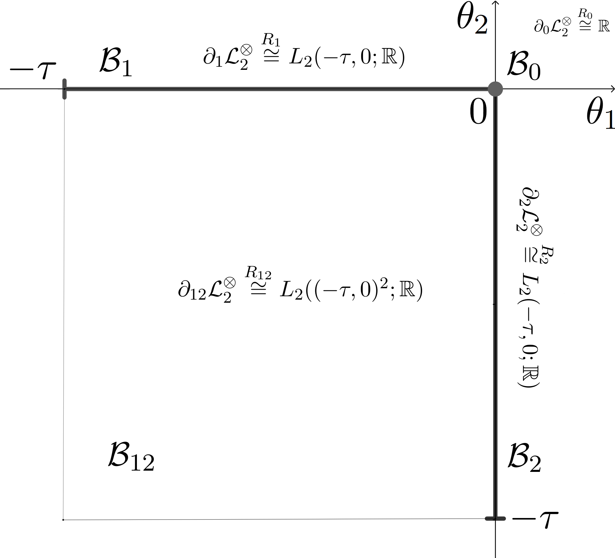
Figure 1. An illustration to the decomposition (3.13) for $m=2$ and $n=1$. Here $\mathcal{L}^{\otimes}_{2}=L_{2}([-\tau,0]^{2};\mu^{\otimes 2};\mathbb{R})$ is decomposed into the sum of the boundary subspaces $\partial_{0}\mathcal{L}^{\otimes}_{2}$, $\partial_{1}\mathcal{L}^{\otimes}_{2}$, $\partial_{2}\mathcal{L}^{\otimes}_{2}$ and $\partial_{12}\mathcal{L}^{\otimes}_{2}$ over the faces $\mathcal{B}_{0}$, $\mathcal{B}_{1}$, $\mathcal{B}_{2}$ and $\mathcal{B}_{12}$ respectively. These subspaces are naturally isomorphic to appropriate $L_{2}$-spaces via the restriction operators $R_{0}$, $R_{1}$, $R_{2}$ and $R_{12}$ respectively.

For $m=2$ and $n=1$, any $\Phi\in\mathcal{L}^{\otimes}_{m}$ is determined by its four restrictions: one value $R_{0}\Phi\in\mathbb{R}$, two functions of single variable $R_{1}\Phi,R_{2}\Phi\in L_{2}(-\tau,0;\mathbb{R})$ and one function of two variables $R_{12}\Phi\in L_{2}((-\tau,0)^{2};\mathbb{R})$ (see Fig. 1). Note that even if $R_{12}\Phi$, $R_{1}\Phi$ or $R_{2}\Phi$ have continuous representations, it is not true in general that they need to be related on intersections of faces. In particular, the values $(R_{12}\Phi)(0,0)$, $(R_{1}\Phi)(0)$, $(R_{2}\Phi)(0)$ and $R_{0}\Phi$ need not be related. ∎

In the case of $\Phi\in\mathcal{L}^{\wedge}_{m}$, one can describe the relations from (3.8) in term of the restrictions $R_{j_{1}\ldots j_{k}}\Phi$. This is contained in the following proposition.

Proposition 3.1 (Proposition 4.1, [3]).

An element $\Phi\in\mathcal{L}^{\otimes}_{m}$ belongs to $\mathcal{L}^{\wedge}_{m}$ iff for any $k\in\{0,\ldots,m\}$, any $1\leq j_{1}<\ldots<j_{k}\leq m$ and $\sigma\in\mathbb{S}_{m}$ we have

(3.14) $$\begin{split}(R_{j_{1}\ldots j_{k}}\Phi)(\theta_{j_{1}},\ldots,\theta_{j_{k}})=(-1)^{\sigma}T_{\sigma}(R_{\sigma^{-1}(j_{1})\ldots\sigma^{-1}(j_{k})}\Phi)(\theta_{j_{\overline{\sigma}(1)}},\ldots,\theta_{j_{\overline{\sigma}(k)}}),\\ \text{ for almost all }(\theta_{j_{1}},\ldots,\theta_{j_{k}})\in(-\tau,0)^{k},\end{split}$$

where $\overline{\sigma}\in\mathbb{S}_{k}$ is such that $\sigma^{-1}(j_{\overline{\sigma}(1)})<\ldots<\sigma^{-1}(j_{\overline{\sigma}(k)})$.

In particular, we have that

(3.15) $$R_{j_{1}\ldots j_{k}}\Phi=(-1)^{\sigma}T_{\sigma}R_{1\ldots k}\Phi\text{ for any }\sigma=\begin{pmatrix}1&\ldots&k&\ldots\\ j_{1}&\ldots&j_{k}&\ldots\end{pmatrix}\in\mathbb{S}_{m}.$$

and, as a consequence, for almost all $(\theta_{1},\ldots,\theta_{k})\in(-\tau,0)^{k}$ we have

(3.16) $$(R_{1\ldots k}\Phi)(\theta_{1},\ldots,\theta_{k})\in(\mathbb{R}^{n})^{\otimes k}\otimes(\mathbb{R}^{n})^{\wedge(m-k)}.$$

Since in the case $n=1$ the operator $T_{\sigma}$ becomes identical, $(\mathbb{R}^{n})^{\otimes m}=\mathbb{R}$ for any $m$ and $(\mathbb{R}^{n})^{\wedge(m-k)}=0$ for $m-k>1$, the relations from (3.14) can be simplified as follows.

Corollary 3.1.

For $n=1$ we have that the relations from (3.14) are equivalent to the relations

(3.17) $$\begin{split}&R_{j_{1}\ldots j_{k}}\Phi=0\text{ for all }k\in\{0,\ldots,m-2\},\\ &R_{\widehat{j}}\Phi\text{ is antisymmetric for any }j\in\{1,\ldots,m\},\\ &R_{\widehat{i}}\Phi=(-1)^{j-i}R_{\widehat{j}}\Phi\text{ for }i,j\in\{1,\ldots,m\},\\ &R_{1\ldots m}\Phi\text{ is antisymmetric}.\end{split}$$

We leave the proof as an exercise to the reader (just use (3.15) and (3.16)) and refer to the proof of Proposition 4.2 below, where necessary arguments are applied in a similar context.

Note that the antisymmetric relations (3.14) link each $\partial_{j_{1}\ldots j_{k}}\mathcal{L}^{\otimes}_{m}$ with other boundary subspaces over $k$-faces (i.e. with the same $k$). Thus, it is convenient to define for a given $k\in\{0,\ldots,m\}$ the subspace

(3.18) $$\partial_{k}\mathcal{L}^{\wedge}_{m}:=\left\{\Phi\in\bigoplus\limits_{j_{1}\ldots j_{k}}\mathcal{L}^{\otimes}_{m}\ |\ \Phi\text{ satisfies the relations from }\eqref{EQ: AntisymmetricRelationsGeneral}\right\},$$

where the sum is taken over all $1\leq j_{1}<\ldots<j_{k}\leq m$. We say that $k$ is improper if $\partial_{k}\mathcal{L}^{\wedge}_{m}$ is the zero subspace. Otherwise we say that $k$ is proper. For example, when $n=1$, Corollary 3.1 gives that any $k\leq m-2$ is improper and only $k=m-1$ and $k=m$ are proper.

Clearly, $\mathcal{L}^{\wedge}_{m}$ decomposes into the orthogonal sum of all $\partial_{k}\mathcal{L}^{\wedge}_{m}$ as

(3.19) $$\mathcal{L}^{\wedge}_{m}=\bigoplus_{k=0}^{m}\partial_{k}\mathcal{L}^{\wedge}_{m}.$$

Below we will identify $\mathbb{H}^{\otimes m}$ and $\mathbb{H}^{\wedge m}$ with $\mathcal{L}^{\otimes m}$ and $\mathcal{L}^{\wedge m}$ according to the isomorphism (3.7) and its restriction (3.10) respectively. Moreover, we will use the same notations for the corresponding additive and multiplicative compound operators, semigroups and cocycles induced from the abstract spaces via the isomorphisms.

To describe the infinitesimal generator of the $m$-fold compound cocycle $\Xi_{m}$ in a form similar to (3.5), we need to introduce the corresponding control and measurement operators. It may be convenient for the reader to have in mind the final result (3.40).

3.3. Induced control operators on tensor and exterior products

For $j\in\{1,\ldots,m\}$ we put $\mathbb{R}_{1,j}:=(\mathbb{R}^{n})^{\otimes(j-1)}$, $\mathbb{R}_{2,j}:=(\mathbb{R}^{n})^{\otimes(m-j)}$ and $\mathbb{U}_{j}:=\mathbb{R}_{1,j}\otimes\mathbb{U}\otimes\mathbb{R}_{2,j}$. Here $\mathbb{U}=\mathbb{R}^{r_{1}}$ is endowed with some inner product as it was defined above (3.1).

For any $k\in\{0,\ldots,m-1\}$ and $1\leq j_{1}<\ldots<j_{k}\leq m$ we associate with the operator $\widetilde{B}$ from (3.1) a linear bounded operator $B^{j_{1}\ldots j_{k}}_{j}$ which takes an element $\Phi_{\mathbb{U}}$ from $L_{2}((-\tau,0)^{k};\mathbb{U}_{j})$ to the element from the boundary subspace $\partial_{j_{1}\ldots j_{k}}\mathcal{L}^{\otimes}_{m}$ (see (3.13)) defined as

(3.20) $$\left(B^{j_{1}\ldots j_{k}}_{j}\Phi_{\mathbb{U}}\right)(\theta_{1},\ldots,\theta_{m}):=(\operatorname{Id}_{\mathbb{R}_{1,j}}\otimes\widetilde{B}\otimes\operatorname{Id}_{\mathbb{R}_{2,j}})\Phi_{\mathbb{U}}(\theta_{j_{1}},\ldots,\theta_{j_{k}})$$

for almost all $(\theta_{1},\ldots,\theta_{m})\in\mathcal{B}^{(m)}_{j_{1}\ldots j_{k}}$ in the sense of the $k$-dimensional Lebesgue measure on $\mathcal{B}^{(m)}_{j_{1}\ldots j_{k}}$ (see (3.11)).

Now we define the control space $\mathbb{U}^{\otimes}_{m}$ as the outer orthogonal sum

(3.21) $$\mathbb{U}^{\otimes}_{m}:=\bigoplus_{k=0}^{m-1}\bigoplus_{j_{1}\ldots j_{k}}\bigoplus_{j\notin\{j_{1},\ldots,j_{k}\}}L_{2}((-\tau,0)^{k};\mathbb{U}_{j}),$$

where the indices $j_{1}\ldots j_{k}$ and $j$ are such that $1\leq j_{1}<\ldots<j_{k}\leq m$ and $j\in\{1,\ldots,m\}$. For convenience, we write $\eta=(\eta^{j}_{j_{1}\ldots j_{k}})$ for an element of $\mathbb{U}^{\otimes}_{m}$, where $\eta^{j}_{j_{1}\ldots j_{k}}$ belongs to the corresponding summand from (3.21). Now the control operator $B^{\otimes}_{m}\in\mathcal{L}(\mathbb{U}^{\otimes}_{m};\mathcal{L}^{\otimes}_{m})$ associated with $\widetilde{B}$ is defined as

(3.22) $$B^{\otimes}_{m}\eta:=\sum_{k=0}^{m-1}\sum_{j_{1}\ldots j_{k}}\sum_{j\notin\{j_{1},\ldots,j_{k}\}}B^{j_{1}\ldots j_{k}}_{j}\eta^{j}_{j_{1}\ldots j_{k}}\text{ for }\eta=(\eta^{j}_{j_{1}\ldots j_{k}})\in\mathbb{U}^{\otimes}_{m},$$

where the sum is just a sum in $\mathcal{L}^{\otimes}_{m}$. More precisely, the inner sum is the sum in $\partial_{j_{1}\ldots j_{k}}\mathcal{L}^{\otimes}_{m}$ and the other sums can be understood according to (3.13).

Now we are going to define an analog of $B^{\otimes}_{m}$ for the antisymmetric subspace $\mathcal{L}^{\wedge}_{m}$. Firstly, consider $\eta=(\eta^{j}_{j_{1}\ldots j_{k}})\in\mathbb{U}^{\otimes}_{m}$ satisfying analogous to (3.14) antisymmetric relations. Namely, for all $k\in\{0,\ldots,m-1\}$, $1\leq j_{1}<\ldots<j_{k}\leq m$, $j\notin\{j_{1},\ldots,j_{k}\}$ and any $\sigma\in\mathbb{S}_{m}$ we require $\eta$ to satisfy

(3.23) $$\begin{split}\eta^{j}_{j_{1}\ldots j_{k}}(\theta_{j_{1}},\ldots,\theta_{j_{k}})=(-1)^{\sigma}T_{\sigma^{-1}}\eta^{\sigma(j)}_{\sigma(j_{\overline{\sigma}(1)})\ldots\sigma(j_{\overline{\sigma}(k)})}(\theta_{j_{\overline{\sigma}(1)}},\ldots,\theta_{j_{\overline{\sigma}(k)}})\\ \text{ for almost all }(\theta_{j_{1}},\ldots,\theta_{j_{k}})\in(-\tau,0)^{k},\end{split}$$

where $\overline{\sigma}\in\mathbb{S}_{k}$ is such that $\sigma(j_{\overline{\sigma}(1)})<\ldots<\sigma(j_{\overline{\sigma}(k)})$. Here $T_{\sigma}\colon\mathbb{U}_{j}\to\mathbb{U}_{\sigma(j)}$ is the transposition operator w.r.t. $\sigma\in\mathbb{S}_{m}$ defined analogously to (3.9).

Relations from (3.23) may be simplified in the case of scalar equations, i.e. for $n=1$. For this, we refer to Proposition 4.2 below the text.

Recall that $k\in\{0,\ldots,m\}$ is called improper if $\partial_{k}\mathcal{L}^{\wedge}_{m}$ from (3.18) is zero. Now we define $\mathbb{U}^{\wedge}_{m}$ as

(3.24) $$\begin{split}\mathbb{U}^{\wedge}_{m}:=\{\eta=(\eta^{j}_{j_{1}\ldots j_{k}})\in\mathbb{U}^{\otimes}_{m}\ |\ &\eta\text{ satisfies }\eqref{EQ: ControlSpaceRelationsAntisymmetricCompoundDelay}\text{ and }\\ &\eta^{j}_{j_{1}\ldots j_{k}}=0\text{ for improper }k\}.\end{split}$$

Let $B^{\wedge}_{m}$ denote the restriction to $\mathbb{U}^{\wedge}_{m}$ of the operator $B^{\otimes}_{m}$ from (3.22). By Proposition 6.1 in [3], we have that $B^{\wedge}_{m}$ belongs to $\mathcal{L}(\mathbb{U}^{\wedge}_{m};\mathcal{L}^{\wedge}_{m})$. In fact, in the proof it is shown that $B^{\otimes}_{m}\eta\in\mathcal{L}^{\wedge}_{m}$ provided that $\eta\in\mathbb{U}^{\otimes}_{m}$ satisfies (3.23). For such $\eta$ it is not necessary that $\eta^{j}_{j_{1}\ldots j_{k}}$ is zero for improper $k$. However, the cumulative impact via (3.22) of such components is an element of $\partial_{k}\mathcal{L}^{\wedge}_{m}$ and it must vanish for improper $k$ since $B^{\otimes}_{m}\eta\in\mathcal{L}^{\wedge}_{m}$. This is why we force these components to be zero in the definition (3.24). See Remark 4.2 for a more concrete example.

3.4. Induced measurement operators on tensor and exterior products

Applying the Riesz representation theorem to the operator $C$ from (3.1), we get an $(r_{2}\times n)$-matrix-valued function $\gamma(\cdot)$ of bounded variation on $[-\tau,0]$ such that

(3.25) $$C\phi=\int_{-\tau}^{0}d\gamma(\theta)\phi(\theta)\text{ for each }\phi\in C([-\tau,0];\mathbb{R}^{n}).$$

Recall $\mathbb{R}_{1,j}=(\mathbb{R}^{n})^{\otimes(j-1)}$, $\mathbb{R}_{2,j}=(\mathbb{R}^{n})^{\otimes(m-j)}$ and put $\mathbb{M}_{j}:=\mathbb{R}_{1,j}\otimes\mathbb{M}\otimes\mathbb{R}_{2,j}$, where $\mathbb{M}=\mathbb{R}^{r_{2}}$ as in (3.1). Then for each $k\in\{0,\ldots,m-1\}$, $J\in\{1,\ldots,k+1\}$ and $j\in\{1,\ldots,m\}$ we define an operator $C^{(k)}_{j,J}$ taking a function $\Phi\in C([-\tau,0]^{k+1};(\mathbb{R}^{n})^{\otimes m})$ to an element $C^{(k)}_{j,J}\Phi$ of $C([-\tau,0]^{k};\mathbb{M}_{j})$ given by

(3.26) $$(C^{(k)}_{j,J}\Phi)(\theta_{1},\ldots,\widehat{\theta_{J}},\ldots,\theta_{k+1}):=\int_{-\tau}^{0}d\gamma_{j}(\theta_{J})\Phi(\theta_{1},\ldots,\theta_{k+1}),$$

where $\gamma_{j}(\theta)=\operatorname{Id}_{\mathbb{R}_{1,j}}\otimes\gamma(\theta)\otimes\operatorname{Id}_{\mathbb{R}_{2,j}}$ for $\theta\in[-\tau,0]$.

We need to consider $C^{(k)}_{j,J}$ in a wider context. For this, we define the space $\mathbb{E}_{k+1}((\mathbb{R}^{n})^{\otimes m})$ of all functions $\Phi\in L_{2}((-\tau,0)^{k+1};(\mathbb{R}^{n})^{\otimes m})$ such that for any $j\in\{1,\ldots,k+1\}$ there exists $\Phi^{b}_{j}(\cdot)\in C([-\tau,0];L_{2}((-\tau,0)^{k};(\mathbb{R}^{n})^{\otimes m}))$ satisfying the identity in $L_{2}((-\tau,0)^{k};(\mathbb{R}^{n})^{\otimes m})$ as

(3.27) $${\left.\kern-1.2pt\Phi\vphantom{\big{|}}\right|_{\mathcal{B}^{(k+1)}_{\widehat{j}}+\theta e_{j}}}=\Phi^{b}_{j}(\theta)\text{ for almost all }\theta\in[-\tau,0],$$

where $e_{j}$ is the $j$-th vector in the standard basis in $\mathbb{R}^{k+1}$ and we naturally identify $\mathcal{B}^{(k+1)}_{\widehat{j}}+\theta e_{j}$ with $(-\tau,0)^{k}$ by omitting the $j$-th coordinate.

In the above notations, we endow the space $\mathbb{E}_{k+1}((\mathbb{R}^{n})^{\otimes m})$ with the norm

(3.28) $$\|\Phi\|_{\mathbb{E}_{k+1}((\mathbb{R}^{n})^{\otimes m})}:=\sup_{1\leq j\leq k+1}\sup_{\theta\in[-\tau,0]}\|\Phi^{b}_{j}(\theta)\|_{L_{2}((-\tau,0)^{k};(\mathbb{R}^{n})^{\otimes m})}$$

that clearly makes it a Banach space. We also put $\mathbb{E}_{0}((\mathbb{R}^{n})^{\otimes m}):=(\mathbb{R}^{n})^{\otimes m}$.

Since $\Phi^{b}_{j}(\theta)$ continuously depend on $\theta\in[-\tau,0]$, it is not hard to show that $C([-\tau,0]^{k+1};(\mathbb{R}^{n})^{\otimes m})$ is dense in $\mathbb{E}_{k+1}((\mathbb{R}^{n})^{\otimes m})$. We have the following proposition.

Proposition 3.2 (Theorem A.3, [3]).

The operator $C^{(k)}_{j,J}$ from (3.26) can be extended to a bounded operator from $\mathbb{E}_{k+1}((\mathbb{R}^{n})^{\otimes m})$ to $L_{2}((-\tau,0)^{k};\mathbb{M}_{j})$. Moreover, its norm does not exceed the total variation $\operatorname{Var}_{[-\tau,0]}(\gamma)$ of $\gamma$ on $[-\tau,0]$, where $\gamma$ is given by (3.25).

Now we define a Banach space $\mathbb{E}^{\otimes}_{m}$ by the outer direct sum as

(3.29) $$\mathbb{E}^{\otimes}_{m}:=\bigoplus_{k=0}^{m}\bigoplus_{j_{1}\ldots j_{k}}\mathbb{E}_{k}((\mathbb{R}^{n})^{\otimes m}),$$

where the inner sum is taken over all $1\leq j_{1}<\ldots<j_{k}\leq m$. We endow $\mathbb{E}^{\otimes}_{m}$ with any of standard norms and embed it into $\mathcal{L}^{\otimes}_{m}$ by naturally sending each element from the $j_{1}\ldots j_{k}$-th summand in (3.29) to the boundary subspace $\partial_{j_{1}\ldots j_{k}}\mathcal{L}^{\otimes}_{m}$ from (3.13). Moreover, let $\mathbb{E}^{\wedge}_{m}$ be the subspace of $\mathbb{E}^{\otimes}_{m}$ which is mapped into $\mathcal{L}^{\wedge}_{m}$ under the embedding.

Analogously to the control space $\mathbb{U}^{\otimes}_{m}$, we introduce the measurement space $\mathbb{M}^{\otimes}_{m}$ given by the outer orthogonal sum

(3.30) $$\mathbb{M}^{\otimes}_{m}:=\bigoplus_{k=0}^{m-1}\bigoplus_{j_{1}\ldots j_{k}}\bigoplus_{j\notin\{j_{1},\ldots,j_{k}\}}L_{2}((-\tau,0)^{k};\mathbb{M}_{j}),$$

where the second sum is taken over all $1\leq j_{1}<\ldots<j_{k}\leq m$ and in the third sum we additionally require that $j\in\{1,\ldots,m\}$.

For given $k\in\{0,\ldots,m-1\}$, $1\leq j_{1}<\ldots<j_{k}\leq m$ and $j\notin\{j_{1},\ldots,j_{k}\}$, we define $J(j)=J(j;j_{1},\ldots,j_{k})$ as the integer $J$ such that $j$ is the $J$-th element in the set $\{j,j_{1},\ldots,j_{k}\}$ arranged by increasing. Now define the measurement operator $C^{\otimes}_{m}\in\mathcal{L}(\mathbb{E}^{\otimes}_{m};\mathbb{M}^{\otimes}_{m})$ as

(3.31) $$C^{\otimes}_{m}\Phi:=\sum_{k=0}^{m-1}\sum_{j_{1}\ldots j_{k}}\sum_{j\notin\{j_{1},\ldots,j_{k}\}}C^{(k)}_{j,J(j)}R_{jj_{1}\ldots j_{k}}\Phi,$$

where the sum is taken in $\mathbb{M}^{\otimes}_{m}$ according to (3.30) and the action of $C^{(k)}_{j,J(j)}$ is understood in the sense of Proposition 3.2.

Now we define an analog of the above constructions for the antisymmetric case. For this, we consider such elements $M=(M^{j}_{j_{1}\ldots j_{k}})\in\mathbb{M}^{\otimes}_{m}$ that satisfy for all $k\in\{0,\ldots,m-1\}$, $1\leq j_{1}<\ldots<j_{k}\leq m$, $j\notin\{j_{1},\ldots,j_{k}\}$ and any $\sigma\in\mathbb{S}_{m}$ the relations

(3.32) $$\begin{split}M^{j}_{j_{1}\ldots j_{k}}(\theta_{j_{1}},\ldots,\theta_{j_{k}})=(-1)^{\sigma}T_{\sigma^{-1}}M^{\sigma(j)}_{\sigma(j_{\overline{\sigma}(1)})\ldots\sigma(j_{\overline{\sigma}(k)})}(\theta_{j_{\overline{\sigma}(1)}},\ldots,\theta_{j_{\overline{\sigma}(k)}})\\ \text{ for almost all }(\theta_{j_{1}},\ldots,\theta_{j_{k}})\in(-\tau,0)^{k},\end{split}$$

where $\overline{\sigma}\in\mathbb{S}_{k}$ is such that $\sigma(j_{\overline{\sigma}(1)})<\ldots<\sigma(j_{\overline{\sigma}(k)})$. Here $T_{\sigma}\colon\mathbb{M}_{j}\to\mathbb{M}_{\sigma(j)}$ is the transposition operator w.r.t. $\sigma\in\mathbb{S}_{m}$ defined analogously to (3.9).

Now we define $\mathbb{M}^{\wedge}_{m}$ as

(3.33) $$\begin{split}\mathbb{M}^{\wedge}_{m}:=\{M=(M^{j}_{j_{1}\ldots j_{k}})\in\mathbb{M}^{\otimes}_{m}\ |\ &M\text{ satisfies }\eqref{EQ: MeasurementSpaceRelationsAntisymmetricCompoundDelay}\text{ and }\\ &M^{j}_{j_{1}\ldots j_{k}}=0\text{ for improper }k\}.\end{split}$$

Let $C^{\wedge}_{m}$ be the restriction of $C^{\otimes}_{m}$ to $\mathbb{E}^{\wedge}_{m}$. Similarly to the operator $B^{\wedge}_{m}$, it can be shown that $C^{\wedge}_{m}$ belongs to $\mathcal{L}(\mathbb{E}^{\wedge}_{m};\mathbb{M}^{\wedge}_{m})$.

3.5. Infinitesimal description of compound cocycles

For any $\wp\in\mathcal{P}$, $k\in\{0,\ldots,m-1\}$ and $j\in\{1,\ldots,m\}$, we consider an induced by $F^{\prime}(\wp)$ from (3.1) operator $F^{\prime}_{j}(\wp)$ which takes $\Phi_{\mathbb{M}}\in L_{2}((-\tau,0)^{k};\mathbb{M}_{j})$ to an element $F^{\prime}_{j}(\wp)\Phi_{\mathbb{M}}$ from $L_{2}((-\tau,0)^{k};\mathbb{U}_{j})$ given by

(3.34) $$(F^{\prime}_{j}(\wp)\Phi_{\mathbb{M}})(\theta_{1},\ldots,\theta_{k}):=(\operatorname{Id}_{\mathbb{R}_{1,j}}\otimes F^{\prime}(\wp)\otimes\operatorname{Id}_{\mathbb{R}_{2,j}})\Phi_{\mathbb{M}}(\theta_{1},\ldots,\theta_{k}),$$

where, as usual, $\mathbb{R}_{1,j}=(\mathbb{R}^{n})^{\otimes(j-1)}$, $\mathbb{R}_{2,j}=(\mathbb{R}^{n})^{\otimes(m-j)}$ and $\mathbb{U}_{j}=\mathbb{R}_{1,j}\otimes\mathbb{U}\otimes\mathbb{R}_{2,j}$ with $\mathbb{U}$ defined above (3.1). Note that we omit the dependence of $F^{\prime}_{j}(\wp)$ on $k$ for convenience.

These operators induce an operator $F^{\otimes}_{m}(\wp)$ from $\mathbb{M}^{\otimes}_{m}$ to $\mathbb{U}^{\otimes}_{m}$ for $M=(M^{j}_{j_{1}\ldots j_{k}})\in\mathbb{M}^{\otimes}_{m}$ given by

(3.35) $$F^{\otimes}_{m}M=\sum_{k=0}^{m-1}\sum_{j_{1}\ldots j_{k}}\sum_{j\notin\{j_{1}\dots j_{k}\}}F^{\prime}_{j}(\wp)M^{j}_{j_{1}\ldots j_{k}},$$

where the second sum is taken over all $1\leq j_{1}<\ldots<j_{k}\leq m$ and in the third sum we additionally require $j\in\{1,\ldots,m\}$. Note that the overall sum is taken in $\mathbb{U}^{\otimes}_{m}$ according to (3.21). Moreover, restricting $F^{\otimes}_{m}(\wp)$ to $\mathbb{M}^{\wedge}_{m}$ gives a well-defined mapping $F^{\wedge}_{m}(\wp)$ into $\mathbb{U}^{\wedge}_{m}$.

Recall that $A$ given by (3.4) is the generator of a $C_{0}$-semigroup in $\mathbb{H}$. Let $A^{[\otimes m]}$ be the $m$-fold additive compound of $A$. Since we identified $\mathbb{H}^{\otimes m}$ with $\mathcal{L}^{\otimes}_{m}$ via the isomorphism from (3.7), it is reasonable to give the description of $A^{[\otimes m]}$ (in particular, $A^{[\wedge m]}$) in terms of the space $\mathcal{L}^{\otimes}_{m}$.

For this, for any $k=1,\ldots,m$ we consider the diagonal Sobolev space $\mathcal{W}^{2}_{D}((-\tau,0)^{k};(\mathbb{R}^{n})^{\otimes m})$ consisting of all $\Phi\in L_{2}((-\tau,0)^{k};(\mathbb{R}^{n})^{\otimes m})$ having a square-summable diagonal derivative (in the generalized sense), i.e.

(3.36) $$\sum_{j=1}^{k}\frac{d}{d\theta_{j}}\Phi\in L_{2}((-\tau,0)^{k};(\mathbb{R}^{n})^{\otimes m}).$$

It can be shown that the space $\mathcal{W}^{2}_{D}((-\tau,0)^{k};(\mathbb{R}^{n})^{\otimes m})$ being endowed with the standard norm is a Hilbert space which is naturally continuously embedded into the space $\mathbb{E}_{k}((\mathbb{R}^{n})^{\otimes m})$ from (3.28) (see Proposition A.1 in [3]).

Analogously to the operators $C^{(k)}_{j,J}$ from (3.26) one can define the operators $\widetilde{A}^{(k)}_{j,J}$ associated with $\widetilde{A}$ from (3.1). Then we have the following theorem.

Theorem 3.1 (Theorem 4.2, Theorem 4.3, [3]).

For the $m$-fold additive compound $A^{[\otimes m]}$ of $A$ given by (3.4) we have that each $\Phi\in\mathcal{D}(A^{[\otimes m]})$ satisfies $R_{j_{1}\ldots j_{k}}\Phi\in\mathcal{W}^{2}_{D}((-\tau,0)^{k};(\mathbb{R}^{n})^{\otimes m})$ for any $k\in\{1,\ldots,m\}$ and $1\leq j_{1}<\ldots<j_{k}\leq m$. Moreover, for such $\Phi$ and any $k\in\{0,\ldots,m\}$ and $1\leq j_{1}<\ldots<j_{k}\leq m$ we have

(3.37) $$R_{j_{1}\ldots j_{k}}\left(A^{[\otimes m]}\Phi\right)=\sum_{l=1}^{k}\frac{\partial}{\partial\theta_{l}}R_{j_{1}\ldots j_{k}}\Phi+\sum_{j\notin\{j_{1},\ldots,j_{k}\}}\widetilde{A}^{(k)}_{j,J(j)}R_{jj_{1}\ldots j_{k}}\Phi,$$

where in the latter sum it is additionally required that $j\in\{1,\ldots,m\}$. Moreover, the graph norm on $\mathcal{D}(A^{\otimes m})$ is equivalent to the norm

(3.38) $$\|\Phi\|^{2}_{\mathcal{W}^{2}_{D}}:=\sum_{k=1}^{m}\sum_{j_{1}\ldots j_{k}}\|R_{j_{1}\ldots j_{k}}\Phi\|^{2}_{\mathcal{W}^{2}_{D}((-\tau,0)^{k};(\mathbb{R}^{n})^{\otimes m})},$$

where $\|\cdot\|_{\mathcal{W}^{2}_{D}((-\tau,0)^{k};(\mathbb{R}^{n})^{\otimes m})}$ is the norm in $\mathcal{W}^{2}_{D}((-\tau,0)^{k};(\mathbb{R}^{n})^{\otimes m})$ and the inner sum is taken over all $1\leq j_{1}<\ldots<j_{k}\leq m$.

Remark 3.2.

Theorem 3.1 does not fully describe the domain $\mathcal{D}(A^{[\otimes m]})$. In fact, functions from the diagonal Sobolev space $\mathcal{W}^{2}_{D}((-\tau,0)^{k};(\mathbb{R}^{n})^{\otimes m})$ have well-defined $L_{2}$-traces on sections of $[-\tau,0]^{k}$ by hyperplanes transversal to the diagonal line in $\mathbb{R}^{k}$. Then for each $\Phi\in\mathcal{D}(A^{[\otimes m]})$ the trace of $R_{j_{1}\ldots j_{k}}\Phi$ on $\mathcal{B}^{(k)}_{\widehat{l}}$ agrees with the restriction $R_{j_{1}\ldots\widehat{j_{l}}\ldots j_{k}}\Phi$ for any $l\in\{1,\ldots,k\}$. This is what is proved in Theorems 4.2 and 4.3 from [3]. We shall not get into details of this fact in the present work, although we will remind it in the proof of Proposition 4.4. Moreover, this agreement of traces and restrictions completely characterize the domain $\mathcal{D}(A^{[\otimes m]})$.

In particular, we have the following continuous embeddings

(3.39) $$\mathcal{D}(A^{[\otimes m]})\subset\mathbb{E}^{\otimes}_{m}\subset\mathcal{L}^{\otimes}_{m}\text{ and }\mathcal{D}(A^{[\wedge m]})\subset\mathbb{E}^{\wedge}_{m}\subset\mathcal{L}^{\wedge}_{m},$$

where the intermediate (or auxiliary) Banach spaces $\mathbb{E}^{\otimes}_{m}$ and $\mathbb{E}^{\wedge}_{m}$ are important for our study (see Theorems 3.2 and 4.1).

Now we are ready to give the infinitesimal description of the $m$-fold multiplicative compound $\Xi_{m}$ of $\Xi$ in the antisymmetric space $\mathcal{L}^{\wedge}_{m}$ as

(3.40) $$\dot{\Phi}(t)=A^{[\wedge m]}\Phi(t)+B^{\wedge}_{m}F^{\wedge}_{m}(\pi^{t}(\wp))C^{\wedge}_{m}\Phi(t).$$

By Theorem 6.1 in [3], we have that for any $\Phi_{0}=\xi_{1}\wedge\ldots\wedge\xi_{m}$ with $\xi_{1},\ldots,\xi_{m}\in\mathcal{D}(A)$ there exists a classical solution, i.e. $\Phi(\cdot)\in C^{1}([0,\infty);\mathcal{L}^{\wedge}_{m})\cap C([0,\infty);\mathcal{D}(A^{[\wedge m]}))$ such that $\Phi(0)=\Phi_{0}$ and $\Phi(t)$ satisfies (3.40) and it is given by the trajectory of $\Xi_{m}$ over $\wp$, i.e. $\Xi^{t}_{m}(\wp,\Phi_{0})=\Phi(t)$ for $t\geq 0$. Consequently, on a dense subset of $\mathcal{L}^{\wedge}_{m}$, the trajectories of $\Xi_{m}$ are classical solutions to (3.40).

3.6. Frequency conditions for the uniform exponential stability of compound cocycles

To describe conditions for the uniform exponential stability of $\Xi_{m}$, we consider it as a nonautonomous perturbation of the $C_{0}$-semigroup $G^{\wedge m}$ generated by $A^{[\wedge m]}$. From this view, (3.40) describes the generator of $\Xi_{m}$ as a nonautonomous boundary perturbation of $A^{[\wedge m]}$.

We are going to consider quadratic constraints concerned with such perturbations. For this, Let $\mathcal{G}(M,\eta)$ be a bounded quadratic form of $M\in\mathbb{M}^{\wedge}_{m}$ and $\eta\in\mathbb{U}^{\wedge}_{m}$. Then we consider a quadratic form $\mathcal{F}$ on $\mathbb{E}^{\wedge}_{m}\times\mathbb{U}^{\wedge}_{m}$ defined as

(3.41) $$\mathcal{F}(\Phi,\eta):=\mathcal{G}(C^{\wedge}_{m}\Phi,\eta)\text{ for }\Phi\in\mathbb{E}^{\wedge}_{m}\text{ and }\eta\in\mathbb{U}^{\wedge}_{m}.$$

We say that $\mathcal{F}$ defines a quadratic constraint for (3.40) if $\mathcal{F}(\Phi,\eta)\geq 0$ for any $\eta=F^{\wedge}_{m}(\wp)C^{\wedge}_{m}\Phi$ with arbitrary $\Phi\in\mathbb{E}^{\wedge}_{m}$ and $\wp\in\mathcal{P}$ and, in addition, $\mathcal{F}(\Phi,0)\geq 0$.

Let us describe the Hermitian extension $\mathcal{F}^{\mathbb{C}}$ of $\mathcal{F}$ defined on the complexifications $(\mathbb{E}^{\wedge}_{m})^{\mathbb{C}}$ and $(\mathbb{U}^{\wedge}_{m})^{\mathbb{C}}$ of $\mathbb{E}^{\wedge}_{m}$ and $\mathbb{U}^{\wedge}_{m}$ respectively as $\mathcal{F}^{\mathbb{C}}(\Phi_{1}+i\Phi_{2},\eta_{1}+i\eta_{2}):=\mathcal{F}(\Phi_{1},\eta_{1})+\mathcal{F}(\Phi_{2},\eta_{2})$ for any $\Phi_{1},\Phi_{2}\in\mathbb{E}^{\wedge}_{m}$ and $\eta_{1},\eta_{2}\in\mathbb{U}^{\wedge}_{m}$. Any $\mathcal{G}$ as above can be represented as

(3.42) $$\mathcal{G}(M,\eta)=(M,\mathcal{G}_{1}M)_{\mathbb{M}^{\wedge}_{m}}+(\eta,\mathcal{G}_{2}M)_{\mathbb{U}^{\wedge}_{m}}+(\eta,\mathcal{G}_{3}\eta)_{\mathbb{U}^{\wedge}_{m}},$$

where $\mathcal{G}_{1}\in\mathcal{L}(\mathbb{M}^{\wedge}_{m})$ and $\mathcal{G}_{3}\in\mathcal{L}(\mathbb{U}^{\wedge}_{m})$ are self-adjoint and $\mathcal{G}_{2}\in\mathcal{L}(\mathbb{M}^{\wedge}_{m};\mathbb{U}^{\wedge}_{m})$. Then for any $\Phi\in(\mathbb{M}^{\wedge}_{m})^{\mathbb{C}}$ and $\eta\in(\mathbb{U}^{\wedge}_{m})^{\mathbb{C}}$ the value $\mathcal{F}^{\mathbb{C}}(\Phi,\eta)$ is given by

(3.43) $$\begin{split}\mathcal{F}^{\mathbb{C}}(\Phi,\eta)=\mathcal{G}^{\mathbb{C}}(C^{\wedge}_{m}\Phi,\eta)=\\ =(C^{\wedge}_{m}\Phi,\mathcal{G}_{1}C^{\wedge}_{m}\Phi)_{(\mathbb{M}^{\wedge}_{m})^{\mathbb{C}}}+\operatorname{Re}(\eta,\mathcal{G}_{2}C^{\wedge}_{m}\Phi)_{(\mathbb{U}^{\wedge}_{m})^{\mathbb{C}}}+(\eta,\mathcal{G}_{3}\eta)_{(\mathbb{U}^{\wedge}_{m})^{\mathbb{C}}},\end{split}$$

where we omitted mentioning complexifications of the operators $C^{\wedge}_{m}$, $\mathcal{G}_{1}$, $\mathcal{G}_{2}$ and $\mathcal{G}_{3}$ for convenience.

With each such $\mathcal{F}$ and $\nu_{0}\in\mathbb{R}$ we associate the following frequency inequality on the line $-\nu_{0}+i\mathbb{R}$ avoiding the spectrum of $A^{[\wedge m]}$.

(FI):

For some $\delta>0$ and any $p$ with $\operatorname{Re}p=-\nu_{0}$ we have

(3.44) $$\mathcal{F}^{\mathbb{C}}(-(A^{[\wedge m]}-pI)^{-1}B^{\wedge}_{m}\eta,\eta)\leq-\delta\left|\eta\right|^{2}_{(\mathbb{U}^{\wedge}_{m})^{\mathbb{C}}}\text{ for any }\eta\in\left(\mathbb{U}^{\wedge}_{m}\right)^{\mathbb{C}}.$$

Recall that $A$ generates an eventually compact semigroup $G$. Then $G^{\otimes m}$ (and, consequently, $G^{\wedge m}$) is also eventually compact. In particular, the spectrum of $A^{[\wedge m]}$ consists of eigenvalues with finite algebraic multiplicity. Let $s(A^{[\wedge m]})$ be the spectral bound of $A^{[\wedge m]}$, i.e. the largest real part of its eigenvalues. According to Proposition 2.1, the value $s(A^{[\wedge m]})$ can be described as the sum of the first $m$ eigenvalues of $A$ if $A$ has at least $m$ eigenvalues or $s(A^{[\wedge m]})=-\infty$ otherwise.

We have the following theorem.

Theorem 3.2 (Theorem 6.2, [3]).

Let $\mathcal{F}$ as in (3.41) define a quadratic constraint for (3.40). Suppose that there exists $\nu_{0}\in\mathbb{R}$ such that $-\nu_{0}>s(A^{[\wedge m]})$ and (FI) is satisfied. Then there exists a bounded self-adjoint operator $P\in\mathcal{L}(\mathcal{L}^{\wedge}_{m})$ such that its quadratic form $V(\Phi):=(\Phi,P\Phi)_{\mathcal{L}^{\wedge}_{m}}$ is positive-definite and for some $\delta_{V}>0$ the cocycle $\Xi_{m}$ in $\mathcal{L}^{\wedge}_{m}$ generated by (3.40) satisfies

(3.45) $$e^{2\nu_{0}t}V(\Xi^{t}_{m}(\wp,\Phi))-V(\Phi)\leq-\delta_{V}\int_{0}^{t}e^{2\nu_{0}s}\left|\Xi^{s}_{m}(\wp,\Phi)\right|^{2}_{\mathcal{L}^{\wedge}_{m}}ds.$$

for any $t\geq 0$, $\wp\in\mathcal{P}$ and $\Phi\in\mathcal{L}^{\wedge}_{m}$.

Proof.

Let us give a sketch of the proof. For the existence of $P$, we apply Theorem 2.1 from [1] to the pair $(A^{[\wedge m]}+\nu_{0}I,B^{\wedge}_{m})$ and the quadratic form $\mathcal{F}$. There are three key elements which constitute its conditions. Namely,

1. Well-posedness of the integral quadratic functional associated with $\mathcal{F}$ and its computation via the Fourier transform which is discussed around Lemma 6.2 in [3]. This is related to the most heavy part of the theory concerned with the structural Cauchy formula for linear inhomogeneous problems associated with $A^{[\wedge m]}+\nu_{0}I$ and its relation to pointwise measurement operators constituting the functional;

2. Boundedness of the resolvent of $A^{[\wedge m]}+\nu_{0}I$ in $\mathcal{L}(\mathcal{L}^{\wedge}_{m};\mathbb{E}^{\wedge}_{m})$ uniformly on the line $-\nu_{0}+i\mathbb{R}$ which is shown in Corollary 6.1 from [3] (see also Theorem 4.1 and Remark 4.1 of the present paper);

3. Validity of the frequency inequality (3.44).

After Theorem 2.1 from [1] is applied, the proof of (3.45) is standard. ∎

From (3.45) we have that the cocycle $\Xi_{m}$ has a uniform exponential growth with the exponent $\nu_{0}$. This is contained in the following corollary.

Corollary 3.2.

Under (3.45) there exists a constant $M>0$ such that for any $\Phi\in\mathcal{L}^{\wedge}_{m}$ and $\wp\in\mathcal{P}$ we have

(3.46) $$|\Xi^{t}_{m}(\wp,\Phi)|_{\mathcal{L}^{\wedge}_{m}}\leq Me^{-\nu_{0}t}|\Phi|_{\mathcal{L}^{\wedge}_{m}}\text{ for all }t\geq 0.$$

In particular, for $\nu_{0}>0$, the cocycle $\Xi_{m}$ is uniformly exponentially stable with the exponent $\nu_{0}$.

Proof.

Since $\Xi_{m}$ is uniformly continuous, the value

(3.47) $$M_{\Xi}:=\sup_{\wp\in\mathcal{P}}\sup_{s\in[0,1]}\|\Xi^{s}_{m}(\wp,\cdot)\|_{\mathcal{L}(\mathcal{L}^{\wedge}_{m})}$$

is finite. Then from the cocycle property for any $\Phi\in\mathcal{L}^{\wedge}_{m}$, $\wp\in\mathcal{P}$, $t\geq 0$ and $s_{0}\in[t,t+1]$ we have

(3.48) $$|\Xi^{t+1}_{m}(\wp,\Phi)|_{\mathcal{L}^{\wedge}_{m}}=|\Xi^{t+1-s_{0}}(\pi^{s_{0}}(\wp),\Xi^{s_{0}}_{m}(\wp,\Phi))|_{\mathcal{L}^{\wedge}_{m}}\leq M_{\Xi}\cdot|\Xi^{s_{0}}_{m}(\wp,\Phi)|_{\mathcal{L}^{\wedge}_{m}}.$$

Moreover, since $V(\cdot)$ is positive-definite, from (3.45), the Mean Value Theorem and (3.48) for any $t\geq 0$ we get

(3.49) $$\begin{split}\delta^{-1}_{V}V(\Phi)\geq\int_{0}^{\infty}e^{2\nu_{0}s}|\Xi^{s}_{m}(\wp,\Phi)|^{2}_{\mathcal{L}^{\wedge}_{m}}ds\geq\int_{t}^{t+1}e^{2\nu_{0}s}|\Xi^{s}_{m}(\wp,\Phi)|^{2}_{\mathcal{L}^{\wedge}_{m}}ds=\\ =e^{2\nu_{0}s_{0}}|\Xi^{s_{0}}_{m}(\wp,\Phi)|^{2}_{\mathcal{L}^{\wedge}_{m}}\geq e^{2\nu_{0}t}(eM_{\Xi})^{-2}|\Xi^{t+1}_{m}(\wp,\Phi)|^{2}_{\mathcal{L}^{\wedge}_{m}},\end{split}$$

where $s_{0}\in[t,t+1]$. From this we have (3.46) for a proper $M>0$. The proof is finished. ∎

Remark 3.3.

Note that (3.46) implies that the largest uniform Lyapunov exponent $\lambda_{1}(\Xi_{m})$ of $\Xi_{m}$ satisfies $\lambda_{1}(\Xi_{m})\leq-\nu_{0}$ or, equivalently,

(3.50) $$\lambda_{1}(\Xi)+\ldots+\lambda_{m}(\Xi)\leq-\nu_{0},$$

where $\lambda_{1}(\Xi)\geq\lambda_{2}(\Xi)\geq\ldots$ are the uniform Lyapunov exponents of $\Xi$ defined by induction from the relations $\lambda_{1}(\Xi)+\ldots+\lambda_{k}(\Xi)=\lambda_{1}(\Xi_{k})$ for $k=1,2,\ldots$ (see [2, 25]). In [2], it is shown that the largest uniform exponent of $\Xi_{m}$ is upper semicontinuous w.r.t. $\Xi$ in an appropriate topology. In applications, where $\mathcal{P}$ is a positively invariant region for $\pi$ localizing an attractor and $\Xi$ is the linearization cocycle for $\pi$ in this region, this gives the upper semicontinuity w.r.t. $C^{1}$-perturbations of $\pi$ preserving the invariance of the region $\mathcal{P}$. In particular, for $\nu_{0}>0$ the inequality (3.50) gives the negativity of the sum that is preserved under smallness of such perturbations. As we have discussed in the introduction, this is the condition that is verified in the works concerned with generalizations of the Bendixson-Dulac criterion due to R.A. Smith [23]; M.Y. Li and J.S. Muldowney [17, 18, 19]; G.A. Leonov and V.A. Boichenko [16] and others.

There is a natural choice of a quadratic constraint $\mathcal{F}$ for general $F^{\prime}(\cdot)$ satisfying (3.2). Namely, for $\Phi\in\mathbb{E}^{\wedge}_{m}$ and $\eta\in\mathbb{U}^{\wedge}_{m}$ we put

(3.51) $$\mathcal{F}(\Phi,\eta)=\Lambda^{2}|C^{\wedge}_{m}\Phi|^{2}_{\mathbb{M}^{\wedge}_{m}}-|\eta|^{2}_{\mathbb{U}^{\wedge}_{m}}.$$

To see that it is indeed a quadratic constraint, note that $\eta=F^{\otimes}_{m}(\wp)C^{\otimes}_{m}\Phi$ with $\Phi\in\mathbb{E}^{\otimes}_{m}$ according to (3.31) and (3.35) is equivalent to

(3.52) $$\eta^{j}_{j_{1}\ldots j_{k}}=F^{\prime}_{j}(\wp)C^{(k)}_{j,J(j)}R_{jj_{1}\ldots j_{k}}\Phi$$

for any $k\in\{0,\ldots,m-1\}$, $1\leq j_{1}<\ldots<j_{k}\leq m$ and $j\notin\{j_{1},\ldots,j_{k}\}$. Here the norm of each operator $F^{\prime}_{j}(\wp)$ admits the same estimate as $F^{\prime}(\wp)$, i.e. $\leq\Lambda$, due to its definition in (3.34). From this and the definitions of $\mathbb{U}^{\otimes}_{m}$ and $\mathbb{M}^{\otimes}_{m}$ (see (3.21) and (3.30)) it follows that $\mathcal{F}(\Phi,\eta)\geq 0$ for such $\Phi$ and $\eta$. Since the inequality $\mathcal{F}(\Phi,0)\geq 0$ is obvious, $\mathcal{F}$ indeed defines a quadratic constraint for (3.40).

In terms of the transfer operator $W(p):=-C^{\wedge}_{m}(A^{[\wedge m]}-pI)^{-1}B^{\wedge}_{m}$ the frequency inequality (3.44) associated with $\mathcal{F}$ from (3.51) takes the form

(3.53) $$\sup_{\omega\in\mathbb{R}}\|W(-\nu_{0}+i\omega)\|_{(\mathbb{U}^{\wedge}_{m})^{\mathbb{C}}\to(\mathbb{M}^{\wedge}_{m})^{\mathbb{C}}}<\Lambda^{-1}.$$

Note that the norms of $(A^{[\wedge m]}-pI)^{-1}$ for $p=-\nu_{0}+i\omega$ in $\mathcal{L}(\mathcal{L}^{\wedge}_{m};\mathbb{E}^{\wedge}_{m})$ are bounded uniformly in $\omega\in\mathbb{R}$ (see Theorem 4.1 below). From this it is clear that (3.53) is satisfied for all sufficiently small $\Lambda>0$. This reflects the general circumstance that the uniform exponential stability (of the semigroup $G^{\wedge m}$ in our case) is preserved under uniformly small perturbations (controlled by $\Lambda$ in our case).

In general, (3.44) (in particular, (3.53)) represents a nonlocal condition which may be useful to verify in particular problems. From (3.37) it is clear that computation of such conditions requires solving a first-order PDE with boundary conditions containing both partial derivatives and delays. This makes it hard study the problem purely analytically. Moreover, solutions to such problems belong to the domain $\mathcal{D}(A^{[\wedge m]})$ and are not usual smooth functions. Therefore, the development of proper numerical methods for studying such problems is required. In the next section, we present an approach to the problem which is appropriate for scalar equations.

4. Computation of frequency inequalities

4.1. Quadratic constraints for self-adjoint derivatives

Before we start developing approximation schemes, let us consider a bit delicate than (3.53) quadratic constraints and the corresponding frequency inequalities. Such constraints arise in the case when in terms of (3.2) we have $\mathbb{M}=\mathbb{U}$ and $F^{\prime}(\wp)$ is a self-adjoint operator. For example, the conditions are satisfied in the study of equations with scalar nonlinearities and measurements.

Let us firstly state an auxiliary lemma.

Lemma 4.1.

Suppose that $S$ is a bounded self-adjoint operator in a real separable Hilbert space $\mathbb{F}$ such that for some constants $\Lambda_{1}\leq\Lambda_{2}$ we have

(4.1) $$\Lambda_{1}(f,f)_{\mathbb{F}}\leq(f,Sf)_{\mathbb{F}}\leq\Lambda_{2}(f,f)_{\mathbb{F}}\text{ for any }f\in\mathbb{F}.$$

Then the quadratic form $\mathcal{G}(f,\eta)$ of $f,\eta\in\mathbb{F}$ given by

(4.2) $$\mathcal{G}(f,\eta):=-\Lambda_{1}\Lambda_{2}(f,f)_{\mathbb{F}}+(\Lambda_{1}+\Lambda_{2})(f,\eta)_{\mathbb{F}}-(\eta,\eta)_{\mathbb{F}}$$

satisfies $\mathcal{G}(f,\eta)\geq 0$ provided that $\eta=Sf$.

Proof.

Using the Spectral Theorem for Bounded Self-Adjoint Operators, we may assume that $\mathbb{F}=L_{2}(\mathcal{X};\mu;\mathbb{R})$, where $(\mathcal{X},\mu)$ is a measure space with $\mu$ being $\sigma$-finite, and $S$ is a multiplication on a $\mu$-essentially bounded function $\varphi$ on $\mathcal{X}$ with $\varphi(x)\in[\Lambda_{1},\Lambda_{2}]$ for $\mu$-almost all $x\in\mathcal{X}$. Putting $\eta=Sf$ in (4.2), we obtain

(4.3) $$\mathcal{G}(f,Sf)=\int_{\mathcal{X}}\left[-\varphi^{2}(x)+(\Lambda_{1}+\Lambda_{2})\varphi(x)-\Lambda_{1}\Lambda_{2}\right]|f(x)|^{2}d\mu(x)\geq 0$$

since the multiplier in the square brackets is nonnegative $\mu$-almost everywhere. The proof is finished. ∎

Now in terms of Section 3 we suppose that $\mathbb{F}:=\mathbb{M}=\mathbb{U}$ and the operator $S:=F^{\prime}(\wp)$ is self-adjoint for each $\wp\in\mathcal{P}$ and satisfies (4.1) for some $\Lambda_{1}\leq 0\leq\Lambda_{2}$ (independent of $\wp$). Then the same holds for $\mathbb{F}:=\mathbb{U}^{\wedge}_{m}=\mathbb{M}^{\wedge}_{m}$ and the operator $S:=F^{\wedge}_{m}(\wp)$ by similar arguments as used near (3.52). Thus, for the quadratic form $\mathcal{G}(M,\eta)$ of $M\in\mathbb{M}^{\wedge}_{m}$ and $\eta\in\mathbb{U}^{\wedge}_{m}$ given by

(4.4) $$\mathcal{G}(M,\eta):=-\Lambda_{1}\Lambda_{2}(M,M)_{\mathbb{M}^{\wedge}_{m}}+(\Lambda_{1}+\Lambda_{2})(M,\eta)_{\mathbb{U}^{\wedge}_{m}}-(\eta,\eta)_{\mathbb{U}^{\wedge}_{m}},$$

the associated quadratic form $\mathcal{F}(\Phi,\eta):=\mathcal{G}(C^{\wedge}_{m}\Phi,\eta)$ of $\Phi\in\mathbb{E}^{\wedge}_{m}$ and $\eta\in\mathbb{U}^{\wedge}_{m}$ defines a quadratic constraint for (3.40) due to Lemma 4.1 and the inequality $\Lambda_{1}\leq 0\leq\Lambda_{2}$.

For the corresponding frequency inequality (3.44) we have to satisfy for some $\delta>0$ and all $p=-\nu_{0}+i\omega$, where $\omega\in\mathbb{R}$, and $\eta\in(\mathbb{U}^{\wedge}_{m})^{\mathbb{C}}$ the inequality

(4.5) $$\Lambda_{1}\Lambda_{2}\left|W(p)\eta\right|^{2}_{(\mathbb{M}^{\wedge}_{m})^{\mathbb{C}}}+(\Lambda_{1}+\Lambda_{2})\operatorname{Re}(W(p)\eta,\eta)_{(\mathbb{U}^{\wedge}_{m})^{\mathbb{C}}}+|\eta|^{2}_{(\mathbb{U}^{\wedge}_{m})^{\mathbb{C}}}\geq\delta|\eta|^{2}_{(\mathbb{U}^{\wedge}_{m})^{\mathbb{C}}}.$$

In the case $\Lambda_{1}=-\Lambda$ and $\Lambda_{2}=\Lambda$ for some $\Lambda>0$, one may see that (4.5) is equivalent to (3.53), i.e.

(4.6) $$\sup_{\omega\in\mathbb{R}}\|W(-\nu_{0}+i\omega)\|_{(\mathbb{U}^{\wedge}_{m})^{\mathbb{C}}\to(\mathbb{M}^{\wedge}_{m})^{\mathbb{C}}}<\Lambda^{-1}.$$

Now let us assume that $\Lambda_{1}=0$ and $\Lambda_{2}=\Lambda>0$ (the case of monotone nonlinearities). Then (4.5) is equivalent to

(4.7) $$\inf_{\omega\in\mathbb{R}}\inf_{\begin{subarray}{c}\eta\in(\mathbb{U}^{\wedge}_{m})^{\mathbb{C}},\\ \eta\not=0\end{subarray}}\frac{\left(S_{W}(-\nu_{0}+i\omega)\eta,\eta\right)_{(\mathbb{U}^{\wedge}_{m})^{\mathbb{C}}}}{|\eta|^{2}_{(\mathbb{U}^{\wedge}_{m})^{\mathbb{C}}}}+\Lambda^{-1}>0,$$

where $S_{W}(p):=\frac{1}{2}(W(p)+W^{*}(p))$ is the additive symmetrization of $W(p)=-C^{\wedge}_{m}(A^{[\wedge m]}-pI)^{-1}B^{\wedge}_{m}$.

In the forthcoming sections, we will develop an approximation scheme to verify (4.6) and (4.7) for $n=r_{1}=r_{2}=1$ (in terms of (3.1)) and report some experimental results. Note also that in our experiments we use only the condition (4.6), which, as it turned out, provides better results. However, (4.7) may be useful in some other applications.

4.2. Approximation scheme: preliminaries

For the computation of (4.6) and (4.7) we have the following obvious lemma (we recall the main part of its proof in (4.47)).

Lemma 4.2.

Suppose $\mathbb{F}$ is a separable complex Hilbert space with an orthonormal basis $\{e_{k}\}_{k\geq 1}$ and let $S$ be a bounded linear operator in $\mathbb{F}$. Consider the orthogonal projector $P_{N}$ onto the linear span of $e_{1},\ldots,e_{N}$. Then as $N\to\infty$ we have

(4.8) $$\alpha_{N}:=\|P_{N}SP_{N}\|_{\mathcal{L}(\mathbb{F})}\to\|S\|_{\mathcal{L}(\mathbb{F})}.$$

Moreover, $\alpha_{N}\leq\alpha_{N+1}$ for any $N=1,2,\ldots$.

We are aimed to apply Lemma 4.2 to the operators $S:=W(p)$ (see (4.6)) or $S:=-S_{W}(p)$ (see (4.7)) for $p=-\nu_{0}+i\omega$ with a fixed $\nu_{0}\in\mathbb{R}$ and all $\omega\in\mathbb{R}$. Note that in this case we have $\alpha_{N}=\alpha_{N}(-\nu_{0}+i\omega)$ and $\alpha=\alpha(-\nu_{0}+i\omega)$ and thus the convergence in (4.8) depends on $\omega$. From Theorem 4.1 below and the First Resolvent Identity it can be shown that

Lemma 4.3 (Lemma 7.2, [3]).

In the above context, the functions $\mathbb{R}\ni\omega\mapsto\alpha_{N}(-\nu_{0}+i\omega)$ and $\mathbb{R}\ni\omega\mapsto\alpha(-\nu_{0}+i\omega)$ are globally Lipschitz with a uniform in $N$ Lipschitz constant.

This implies that $\alpha_{N}(-\nu_{0}+i\omega)$ converges to $\alpha(-\nu_{0}+i\omega)$ as $N\to\infty$ uniformly on compact subsets of $\omega$. However, to verify frequency inequalities we have to investigate them for $\omega$ from the entire $\mathbb{R}$. Below we conjecture that it is sufficient to work on a finite segment due to an asymptotically almost periodic behavior of $\alpha_{N}(-\nu_{0}+i\omega)$ as $|\omega|\to\infty$ (see Conjecture 1).

Thus, from the perspective given by Lemma 4.2, for numerical verification of frequency inequalities it is required to compute $-C^{\wedge}_{m}(A^{[\wedge m]}-pI)^{-1}B^{\wedge}_{m}\eta$ for a finite number of $\eta$ belonging to an orthonormal basis in $(\mathbb{U}^{\wedge}_{m})^{\mathbb{C}}$.

We leave open the problem of developing appropriate numerical schemes for direct computations (i.e. by finite-difference methods or projection methods) of the resolvent via solving the corresponding first-order PDE with boundary conditions on the $m$-cube $(-\tau,0)^{m}$ according to the description of $A^{[\wedge m]}$ from Theorem 3.1.

Below we will develop an alternative approach which works at least for scalar equations. It is concerned with the computation of trajectories of the semigroup $G$ only and relies on the following proposition which is the well-known representation of the resolvent via the Laplace transform of the semigroup. For convenience, hereinafter we use the same notations to denote the complexifications of operators defined in Section 3, but we emphasize complexifications of the spaces.

Proposition 4.1 (Theorem 1.10, Chapter II, [11]).

Suppose that $p\in\mathbb{C}$ is such that $\operatorname{Re}p>\omega(G^{\wedge m})$, where $\omega(G^{\wedge m})$ is the growth bound of $G^{\wedge m}$. Then for any $\Phi\in(\mathcal{L}^{\wedge}_{m})^{\mathbb{C}}$ we have

(4.9) $$-(A^{[\wedge m]}-pI)^{-1}\Phi=\int_{0}^{\infty}e^{-pt}G^{\wedge m}(t)\Phi dt.$$

In particular, for $\psi_{1},\ldots,\psi_{m}\in\mathbb{H}^{\mathbb{C}}$ and $\Phi=\psi_{1}\wedge\ldots\wedge\psi_{m}$ we have

(4.10) $$-(A^{[\wedge m]}-pI)^{-1}(\psi_{1}\wedge\ldots\wedge\psi_{m})=\int_{0}^{\infty}e^{-pt}G(t)\psi_{1}\wedge\ldots\wedge G(t)\psi_{m}dt.$$

Now our aim is to provide proper uniform estimates for the tail of the integral from (4.9). For this, the following fundamental property of additive compound operators arising from delay equations is essential. Recall here the intermediate space $\mathbb{E}^{\wedge}_{m}$ defined below (3.29).

Theorem 4.1 (Theorem 4.4, [3]).

For regular (i.e. non-spectral) points $p\in\mathbb{C}$ of $A^{[\wedge m]}$ we have the estimate

(4.11) $$\|(A^{[\wedge m]}-pI)^{-1}\|_{\mathcal{L}((\mathcal{L}^{\wedge}_{m})^{\mathbb{C}};(\mathbb{E}^{\wedge}_{m})^{\mathbb{C}})}\leq C_{1}(p)\cdot\|(A^{[\wedge m]}-pI)^{-1}\|_{\mathcal{L}((\mathcal{L}^{\wedge}_{m})^{\mathbb{C}})}+C_{2}(p),$$

where the constants $C_{1}(p)$ and $C_{2}(p)$ in fact depend on $\max\{1,e^{-\tau\operatorname{Re}p}\}$ in an increasing manner.

Remark 4.1.

Note that the norms of the resolvent $(A^{[\wedge m]}-pI)^{-1}$ in $\mathcal{L}((\mathcal{L}^{\wedge}_{m})^{\mathbb{C}})$ are uniformly bounded on any vertical line $-\nu_{0}+i\mathbb{R}$, where $\nu_{0}\in\mathbb{R}$, which avoids the spectrum of $A^{[\wedge m]}$. For the case of our interest $-\nu_{0}>\omega(G^{\wedge m})=s(A^{[\wedge m]})$ (the semigroup $G^{\wedge m}$ is eventually compact) this follows directly from (4.9). For the general case this can be shown via spectral decompositions (see, for example, Theorem 4.2 in [1]). Using this and (4.11), we immediately get a uniform bound in $\mathcal{L}((\mathcal{L}^{\wedge}_{m})^{\mathbb{C}};(\mathbb{E}^{\wedge}_{m})^{\mathbb{C}})$.

From this, we derive the following main result that justifies the forthcoming approximation scheme.

Theorem 4.2.

Let $\nu_{0}\in\mathbb{R}$ be such that $-\nu_{0}>\omega(G^{\wedge m})$. Then for $p=-\nu_{0}+i\omega$, where $\omega\in\mathbb{R}$, any $\Phi\in(\mathcal{L}^{\wedge}_{m})^{\mathbb{C}}$ and $T\geq 0$ we have

(4.12) $$-(A^{[\wedge m]}-pI)^{-1}\Phi=\int_{0}^{T}e^{-pt}G^{\wedge m}(t)\Phi dt+R_{T}(p;\Phi),$$

where $R_{T}(p;\Phi)\in\mathcal{D}(A^{[\wedge m]})\subset(\mathbb{E}^{\wedge}_{m})^{\mathbb{C}}$ and for any $\varkappa\in(0,-\nu_{0}-\omega(G^{\wedge m}))$ there exists $M_{\varkappa}>0$ such that $R_{T}$ satisfies the estimate

(4.13) $$\|R_{T}(p;\Phi)\|_{(\mathbb{E}^{\wedge}_{m})^{\mathbb{C}}}\leq M_{\varkappa}e^{-\varkappa T}\cdot|\Phi|_{(\mathcal{L}^{\wedge}_{m})^{\mathbb{C}}}\text{ for any }T\geq 0$$

which is uniform in $p=-\nu_{0}+i\omega$ with $\omega\in\mathbb{R}$.

Proof.

From (4.10) we have that $R_{T}=R_{T}(p;\Phi)$ satisfies

(4.14) $$\begin{split}R_{T}=\int_{T}^{\infty}e^{-pt}G^{\wedge m}(t)\Phi dt=e^{-pT}(A^{[\wedge m]}-pI)^{-1}G^{\wedge m}(T)\Phi.\end{split}$$

Suppose that $\varkappa\in(0,-\nu_{0}-\omega(G^{\wedge m}))$. Then there exists $\widetilde{M}_{\varkappa}>0$ such that

(4.15) $$|G^{\wedge m}(T)\Phi|_{(\mathcal{L}^{\wedge}_{m})^{\mathbb{C}}}\leq\widetilde{M}_{\varkappa}e^{-(\nu_{0}+\varkappa)T}\cdot|\Phi|_{(\mathcal{L}^{\wedge}_{m})^{\mathbb{C}}}$$

is satisfied for any $T\geq 0$ and $\Phi\in(\mathcal{L}^{\wedge}_{m})^{\mathbb{C}}$. Combining this along with (4.14) and (4.11) (see Remark 4.1), we obtain (4.13). The proof is finished. ∎

Now we are going to exploit (4.10) sticking to the case $r_{1}=r_{2}=1$, i.e. $\mathbb{M}=\mathbb{U}=\mathbb{R}$, and $n=1$. In fact, $r_{2}=\dim\mathbb{M}$ can be arbitrary that allows a possibility of several measurements for the operator $C$ and $r_{2}=1$ is considered only for simplicity. However, the restrictions $r_{1}=\dim\mathbb{U}=1$ and $n=1$ are essential and to apply our approach for more general cases, the key step is to derive an analog of Proposition 4.3 below.

We start with the following proposition describing the antisymmetric relations (3.23) in the control space $\mathbb{U}^{\wedge}_{m}$. Clearly, the same description holds for the measurement space $\mathbb{M}^{\wedge}_{m}$. Although we need to describe it only for $k=m-1$ (since all $k\leq m-2$ are improper), we give such a description for any $k$.

Proposition 4.2.

For $n=1$ the relations from (3.23) take the form

(4.16) $$\begin{split}&\eta^{j}_{j_{1}\ldots j_{k}}=0\text{ for all }k\in\{0,\ldots,m-3\},\\ &\eta^{j}_{\widehat{j}}\text{ is antisymmetric for any }j\in\{1,\ldots,m\},\\ &\eta^{j}_{\widehat{j}}=(-1)^{j-i}\eta^{i}_{\widehat{i}}\text{ for any }i,j\in\{1,\ldots,m\},\\ &\eta^{j}_{\widehat{ij}}=-\eta^{i}_{\widehat{ij}}\text{ for any distinct }i,j\in\{1,\ldots,m\},\\ &\eta^{j}_{\widehat{ij}}\text{ is antisymmetric for any distinct }i,j\in\{1,\ldots,m\},\\ &\eta^{j}_{\widehat{ij}}=(-1)^{(k-i)+1}\eta^{j}_{\widehat{kj}}\text{ for any distinct }i,j,k\in\{1,\ldots,m\}.\end{split}$$

Proof.

For $n=1$ we have that $\mathbb{U}_{j}=\mathbb{U}$ (see the beginning of Subsection 3.3) and, consequently, $T_{\sigma}$ in (3.23) is the identity operator. Let us start from $k\in\{0,\ldots,m-3\}$ (of course, if $m\geq 3$). Then we use (3.23) with $j_{l}=l$ for $l\in\{1,\ldots,k\}$, $j=k+1$ and $\sigma\in\mathbb{S}_{m}$ such that

(4.17) $$\sigma=\begin{pmatrix}1&\ldots&k+1&\ldots\\ 1&\ldots&k+1&\ldots\end{pmatrix},$$

where the tail, i.e. $\sigma(l)$ for $l>k+1$, is arbitrary. This leads to

(4.18) $$\eta^{k+1}_{1\ldots k}=(-1)^{\sigma}\eta^{k+1}_{1\ldots k}.$$

Since there are at least $2$ undetermined positions in $\sigma$, by a proper choice of $\sigma$ we obtain $\eta^{k+1}_{1\ldots k}=-\eta^{k+1}_{1\ldots k}$ or $\eta^{k+1}_{1\ldots k}=0$. This shows the first part of (4.16) since any $\eta^{j}_{j_{1}\ldots j_{k}}$ can be determined from $\eta^{k+1}_{1\ldots k}$ due to (3.23).

Now let us consider the case $k=m-1$. Let $j\in\{1,\ldots,m\}$. Then (3.23) takes the form

(4.19) $$\eta^{j}_{\widehat{j}}(\theta_{1},\ldots,\widehat{\theta}_{j},\ldots\theta_{m})=(-1)^{\sigma}\eta^{\sigma(j)}_{\widehat{\sigma(j)}}(\theta_{\sigma^{-1}(1)},\ldots,\widehat{\theta}_{\sigma^{-1}(\sigma(j))},\ldots,\theta_{\sigma^{-1}(m)}).$$

Taking this condition over all $\sigma$ such that $\sigma(j)=j$ gives the antisymmetricity of $\eta^{j}_{\widehat{j}}$, i.e. the second property from (4.16). Moreover, taking the cycle $\sigma=(ij)$ for some $i,j\in\{1,\ldots,m\}$ and utilizing the antisymmetricity gives the third identity from (4.16). It is not hard to show that these two properties are sufficient to derive (4.19) for general permutations.

In the case $k=m-2$, we consider (3.23) with $\sigma=(ij)$ to show the fourth identity from (4.16); $\sigma$ such that $\sigma(i)=i$ and $\sigma(j)=j$ and arbitrarily permuting the remained elements to obtain the fifth property from (4.16); $\sigma=(ik)$ for the sixth identity from (4.16). We leave details to the reader. The proof is finished. ∎

Remark 4.2.

By the fourth series of relations from (4.16), we may illustrate the discussion given below (3.24) on forcing $\eta^{j}_{\widehat{ij}}$ to be zero in the definition (3.24) of $\mathbb{U}^{\wedge}_{m}$. Although single components $\eta^{j}_{\widehat{ij}}$ satisfying the relations need not be zero, the corresponding inner sum in the definition (3.22) of $B^{\otimes}_{m}$ vanish since

(4.20) $$B^{\widehat{ij}}_{i}\eta^{i}_{\widehat{ij}}+B^{\widehat{ij}}_{j}\eta^{j}_{\widehat{ij}}=\widetilde{B}\left(\eta^{i}_{\widehat{ij}}+\eta^{j}_{\widehat{ij}}\right)=0.$$

Thus, these components does not give any effect on the control system.

In virtue of Proposition 4.2, it is convenient to identify any element $\eta\in(\mathbb{U}^{\wedge}_{m})^{\mathbb{C}}$ with an $m$-tuple $\eta=(\eta^{j}_{\widehat{j}})_{j=1}^{m}$, where each $\eta^{j}_{\widehat{j}}$ is an antisymmetric function from $L_{2}((-\tau,0)^{m-1};\mathbb{C})$ and $\eta^{j}_{\widehat{j}}=(-1)^{1-j}\eta^{1}_{\widehat{1}}$ for any $j=1,\ldots,m$. Clearly, this establishes an isometric isomorphism between $(\mathbb{U}^{\wedge}_{m})^{\mathbb{C}}$ and the subspace of such tuples in the orthogonal sum $\bigoplus_{j=1}^{m}L_{2}((-\tau,0)^{m-1};\mathbb{C})$. Since any $\eta^{j}_{\widehat{j}}$ is uniquely determined from $\eta^{1}_{\widehat{1}}$, it is sufficient to construct an orthonormal basis in the subspace of antisymmetric functions from $L_{2}((-\tau,0)^{m-1};\mathbb{C})$.

Consider a family of functions $\phi_{k}(\theta)$, where $k\in\mathbb{Z}$, forming an orthonormal basis in $L_{2}(-\tau,0;\mathbb{C})$. Then the functions $\phi_{k_{1}}(\theta_{1})\cdot\ldots\cdot\phi_{k_{m-1}}(\theta_{m-1})$ taken over all $k_{1},\ldots,k_{m-1}\in\mathbb{Z}$ form an orthonormal basis in the space $L_{2}((-\tau,0)^{m-1};\mathbb{C})$ and the functions

(4.21) $$\begin{split}U_{k_{1}\ldots k_{m-1}}(\theta_{1},\ldots,\theta_{m-1}):=\\ \frac{1}{\sqrt{(m-1)!}}\cdot\sum_{\widetilde{\sigma}\in\mathbb{S}_{m-1}}(-1)^{\widetilde{\sigma}}\phi_{k_{1}}(\theta_{\widetilde{\sigma}(1)})\cdot\ldots\cdot\phi_{k_{m-1}}(\theta_{\widetilde{\sigma}(m-1)})\end{split}$$

taken over all integers $k_{1}<k_{2}<\ldots<k_{m-1}$ form an orthonormal basis in the subspace of antisymmetric functions from $L_{2}((-\tau,0)^{m-1};\mathbb{C})$. Consequently, the $m$-tuples $U^{\wedge}_{k_{1}\ldots k_{m-1}}=(U^{j}_{k_{1}\ldots k_{m-1}})_{j=1}^{m}$, where

(4.22) $$U^{j}_{k_{1}\ldots k_{m-1}}:=(-1)^{1-j}m^{-1/2}U_{k_{1}\ldots k_{m-1}},$$

taken over all integers $k_{1}<k_{2}<\ldots<k_{m-1}$ form an orthonormal basis in the control space $(\mathbb{U}^{\wedge}_{m})^{\mathbb{C}}$.

For $k\in\mathbb{Z}$ let $\psi_{k}\in\mathbb{H}$ be such that $R^{(1)}_{1}\psi_{k}=\phi_{k}$ and $R^{(1)}_{0}\psi_{k}=\phi_{k}(0)$.

Proposition 4.3.

In the context of (3.1) suppose that $n=r_{1}=1$. Then for $U^{\wedge}_{k_{1}\ldots k_{m-1}}=(U^{j}_{k_{1}\ldots k_{m-1}})_{j=1}^{m}$ defined by (4.22) we have

(4.23) $$B^{\wedge}_{m}U^{\wedge}_{k_{1}\ldots k_{m-1}}=\psi_{k_{1}}\wedge\ldots\wedge\psi_{k_{m-1}}\wedge\psi_{\infty},$$

where $\psi_{\infty}\in\mathbb{H}$ is such that $R^{(1)}_{1}\psi_{\infty}\equiv 0$ and

(4.24) $$R^{(1)}_{0}\psi_{\infty}=(-1)^{m+1}\cdot\sqrt{m!}\cdot\widetilde{B}.$$

Proof.

Let $b_{j}\colon\{1,\ldots,m-1\}\to\{1,\ldots,\widehat{j},\ldots,m\}$ be the bijection such that $b_{j}(l)=l$ for $l<j$ and $b_{j}(l)=l+1$ for $l\geq j$. Then from (3.10) for $\mu^{\otimes m}$-almost all $(\theta_{1},\ldots,\theta_{m})\in[-\tau,0]^{m}$ we have

(4.25) $$\begin{split}(\psi_{k_{1}}\wedge\ldots\wedge\psi_{k_{m-1}}\wedge\psi_{\infty})(\theta_{1},\ldots,\theta_{m})=\\ =\frac{1}{m!}\sum_{\sigma\in\mathbb{S}_{m}}(-1)^{\sigma}\cdot\psi_{k_{1}}(\theta_{\sigma(1)})\cdot\ldots\cdot\psi_{k_{m-1}}(\theta_{\sigma(m-1)})\cdot\psi_{\infty}(\theta_{\sigma(m)})=\\ =\frac{1}{m}\sum_{j=1}^{m}\psi_{\infty}(\theta_{j})\frac{1}{(m-1)!}\sum_{\widetilde{\sigma}\in\mathbb{S}_{m-1}}(-1)^{\widehat{\sigma}_{j}}\cdot\psi_{k_{1}}(\theta_{\widetilde{\sigma}_{j}(1)})\cdot\ldots\cdot\psi_{k_{m-1}}(\theta_{\widetilde{\sigma}_{j}(m-1)}),\end{split}$$

where $\widetilde{\sigma}_{j}:=b_{j}\circ\widetilde{\sigma}$ and $\widehat{\sigma}_{j}\in\mathbb{S}_{m}$ is given by

(4.26) $$\widehat{\sigma}_{j}=\begin{pmatrix}1&\ldots&m-1&m\\ \widetilde{\sigma}_{j}(1)&\dots&\widetilde{\sigma}_{j}(m-1)&j\end{pmatrix}.$$

It is easy to see that any inversion $\widehat{\sigma}_{j}(l_{1})>\widehat{\sigma}_{j}(l_{2})$ for some $1\leq l_{1}<l_{2}\leq m-1$ is equivalent to $\widetilde{\sigma}(l_{1})>\widetilde{\sigma}(l_{2})$ and there are exactly $m-j$ inversions in $\widehat{\sigma}_{j}$ for $l_{2}=m$. Thus, $(-1)^{\widehat{\sigma}_{j}}=(-1)^{\widetilde{\sigma}}\cdot(-1)^{m-j}$. Applying the restriction operator $R^{(m)}_{\widehat{j}}$ to (4.25) (only the $j$-th summand survives) and using (4.24) and (4.22), we obtain

(4.27) $$\begin{split}R^{(m)}_{\widehat{j}}(\psi_{k_{1}}\wedge\ldots\wedge\psi_{k_{m-1}}\wedge\psi_{\infty})=R^{(1)}_{0}\psi_{\infty}\cdot\frac{(-1)^{m+1}}{\sqrt{m!}}\cdot U^{j}_{k_{1}\ldots k_{m-1}}=\widetilde{B}U^{j}_{k_{1}\ldots k_{m-1}}.\end{split}$$

that shows (4.23) according to the definition of $B^{\wedge}_{m}$ as the restriction of $B^{\otimes}_{m}$ from (3.22) to $(\mathbb{U}^{\wedge}_{m})^{\mathbb{C}}$. The proof is finished. ∎

Combining Propositions 4.1 and 4.3, we obtain the following.

Corollary 4.1.

In the context of Proposition 4.3 suppose that $p\in\mathbb{C}$ is such that $\operatorname{Re}p>\omega(G^{\wedge m})$. Then for any integers $k_{1}<k_{2}<\ldots<k_{m-1}$ we have

(4.28) $$\begin{split}-(A^{[\wedge m]}-pI)^{-1}B^{\wedge}_{m}U^{\wedge}_{k_{1}\ldots k_{m-1}}=\\ =\int_{0}^{\infty}e^{-pt}G(t)\psi_{k_{1}}\wedge\ldots\wedge G(t)\psi_{k_{m-1}}\wedge G(t)\psi_{\infty}dt=\\ =\int_{0}^{T}e^{-pt}G(t)\psi_{k_{1}}\wedge\ldots\wedge G(t)\psi_{k_{m-1}}\wedge G(t)\psi_{\infty}dt+R_{T},\end{split}$$

where $R_{T}=R_{T}(p;B^{\wedge}_{m}U^{\wedge}_{k_{1}\ldots k_{m-1}})$ admits the exponential decay estimate as in (4.13). In particular, the decay is uniform in $k_{1},\ldots,k_{m-1}\in\mathbb{Z}$ and $\operatorname{Re}p$.

Thus, (4.28) expresses the boundary action (i.e. via $B^{\wedge}_{m}$) of the resolvent of $A^{[\wedge m]}$ on the basis vector $U^{\wedge}_{k_{1}\ldots k_{m-1}}$ through the integral over $[0,T]$ involving solutions $G(t)\psi_{k}$ and $G(t)\psi_{\infty}$ of the linear system corresponding to $A$ plus a term $R_{T}$ which admits a uniform exponential decay as $T\to\infty$. Here $G(t)\psi_{\infty}$ is the fundamental solution up to the multiplier $R^{(1)}_{0}\psi_{\infty}$.

For the computation of the integral from (4.28), we have the following.

Proposition 4.4.

In the context (4.28), suppose that $\phi_{k}\in L_{2}(-\tau,0;\mathbb{C})$ is taken to be continuous for all $k\in\mathbb{Z}$ and put

(4.29) $$\mathcal{I}:=\int_{0}^{T}e^{-pt}G(t)\psi_{k_{1}}\wedge\ldots\wedge G(t)\psi_{k_{m-1}}\wedge G(t)\psi_{\infty}dt\in\mathcal{D}(A^{[\wedge m]}).$$

Then $R^{(m)}_{1\ldots m}\mathcal{I}$ belongs to $C([-\tau,0]^{m};\mathbb{C})$ and

(4.30) $$(R^{(m)}_{1\ldots m}\mathcal{I})(\theta_{1},\ldots,\theta_{m})=\int_{0}^{T}e^{-pt}\bigwedge_{k_{1}\ldots k_{m-1}}(t)(\theta_{1},\ldots,\theta_{m})dt$$

for all $(\theta_{1},\ldots,\theta_{m})\in[-\tau,0]^{m}$, where for $t\in[0,T]$ we have

(4.32) $$\bigwedge_{k_{1}\ldots k_{m-1}}(t):=R^{(1)}_{1}G(t)\psi_{k_{1}}\wedge\ldots\wedge R^{(1)}_{1}G(t)\psi_{k_{m-1}}\wedge R^{(1)}_{1}G(t)\psi_{\infty}.$$

Moreover, $\mathcal{I}$ and $R^{(m)}_{1\ldots m}\mathcal{I}$ coincide $\mu^{\otimes m}$-almost everywhere in $[-\tau,0]^{m}$.

Proof.

Since $R^{(m)}_{1\ldots m}$ is a bounded operator in $\mathcal{L}^{\wedge}_{m}$, from (4.29) and (3.10) we have

(4.33) $$R^{(m)}_{1\ldots m}\mathcal{I}=\int_{0}^{T}e^{-pt}\bigwedge_{k_{1}\ldots k_{m-1}}(t)dt.$$

Now the validity of (4.30) for almost all $(\theta_{1},\ldots,\theta_{m})\in[-\tau,0]^{m}$ is a well-known measure-theoretic fact. Note that for any $k\in\mathbb{Z}$ the function

(4.34) $$x_{k}(t):=\begin{cases}R^{(1)}_{0}G(t)\psi_{k},\ &\text{ if }t\geq 0,\\ \phi_{k}(t),\ &\text{ if }t\in[-\tau,0]\end{cases}$$

is continuous in $t\geq-\tau$ since it is the boundary part of the solution with continuous initial data and $(R^{(1)}_{1}G(t)\psi_{k})(\theta)=x_{k}(t+\theta)$ for all $\theta\in[-\tau,0]$ and $t\geq 0$. Moreover, $x_{\infty}(t)$ (defined by the above formula for $k=\infty$) is continuous in $[-\tau,0)$ and in $t\geq 0$. From this, (4.32) and (4.31) it is clear that the integral in (4.30) can be represented as a finite sum of integrals depending continuously on $(\theta_{1},\ldots,\theta_{m})\in[-\tau,0]^{m}$. Thus the entire integral (and, consequently, $R^{(m)}_{1\ldots m}\mathcal{I}$) belongs to $C([-\tau,0]^{m};\mathbb{C})$.

To show that $\mathcal{I}$ and $R^{(m)}_{1\ldots m}\mathcal{I}$ coincide $\mu^{\otimes m}$-almost everywhere in $[-\tau,0]^{m}$, we use the fact that $\mathcal{I}\in\mathcal{D}(A^{[\wedge m]})$. By Theorem 4.2 in [3], for any $k\in\{1,\ldots,m\}$ and $1\leq j_{1}<\ldots<j_{k}\leq m$ the restriction $R^{(k)}_{j_{1}\ldots j_{k}}\mathcal{I}$ belongs to $\mathcal{W}^{2}_{D}((-\tau,0)^{k};\mathbb{C})$ and has traces on the $k$-faces $\mathcal{B}^{(k)}_{\widehat{l}}$ for $l\in\{1,\ldots,k\}$ which agree in a $L_{2}$-sense with the restrictions of order $k-1$. By Theorem A.2 in [3], taking the trace of a continuous function is equivalent to taking its restriction. Thus, the restriction $R^{(m)}_{\widehat{j}}\mathcal{I}$ belongs to $C([-\tau,0]^{m-1};\mathbb{C})$ since it agrees with the restriction of $R^{(m)}_{1\ldots m}\mathcal{I}$ to $\mathcal{B}^{m}_{\widehat{j}}$ for any $j\in\{1,\ldots,m\}$. One may repeat this argument starting from $R^{(m)}_{\widehat{j}}\mathcal{I}$ and pass to the restrictions of order $m-2$ and so on. Note that they are in fact vanish due to Corollary 3.1. The proof is finished. ∎

4.3. Approximation scheme: statement

Now we are ready to describe an approximation scheme for verification of frequency inequalities from (4.6) and (4.7) in the case of scalar equations. For simplicity, we suppose that the measurement operator $C$ is given by $C\phi=\phi(-\tau_{0})$ for some $\tau_{0}\in[0,\tau]$ and $\phi\in C([-\tau,0];\mathbb{R})$. In the forthcoming applications, we encounter the cases $\tau_{0}=0$ and $\tau_{0}=\tau$.

For convenience, we rewrite (3.1) in the case $n=r_{1}=r_{2}=1$ and $C$ as above. Thus, we have

(4.35) $$\dot{x}(t)=\widetilde{A}x_{t}+\widetilde{B}F^{\prime}(\pi^{t}(\wp))x(t-\tau_{0}),$$

where the operators $\widetilde{B}$ and $F^{\prime}(\wp)$ can be identified with real numbers. Let $\Lambda>0$. Then the frequency condition (4.6) is associated with the case

(4.36) $$|F^{\prime}(\wp)|\leq\Lambda\text{ for all }\wp\in\mathcal{P}$$

and the frequency condition (4.7) is associated with the case

(4.37) $$0\leq F^{\prime}(\wp)\leq\Lambda\text{ for all }\wp\in\mathcal{P}.$$

By the Riesz representation theorem, there exists a function of bounded variation $\alpha(\cdot)$ on $[-\tau,0]$ such that

(4.38) $$\widetilde{A}\phi=\int_{-\tau}^{0}\phi(\theta)d\alpha(\theta)\text{ for any }\phi\in C([-\tau,0];\mathbb{R}).$$

It is well-known that the spectrum of $A$, which is associated with $\widetilde{A}$ via (3.4), is given by the roots $p\in\mathbb{C}$ of

(4.39) $$\int_{-\tau}^{0}e^{p\theta}d\alpha(\theta)-p=0.$$

For example, if $\widetilde{A}\phi=a\phi(0)+b\phi(-\tau)$ for some $a,b\in\mathbb{R}$, then (4.39) takes the form $a+be^{-\tau p}-p=0$. Let $\lambda_{1}(A)$, $\lambda_{2}(A)$, …be the eigenvalues of $A$ arranged by nonincreasing of real parts and according to their multiplicity. By Proposition 2.1, the spectral bound $s(A^{[\wedge m]})$ of $A^{[\wedge m]}$ is given by $\sum_{j=1}^{m}\lambda_{j}(A)$ or, if there are less than $m$ eigenvalues, $-\infty$.

Below, as the orthonormal system we take $\phi_{k}(\theta)=\tau^{-1/2}\exp(i\tau^{-1}2\pi k\theta)$, although it is only essential that each function $\phi_{k}$ is continuous. So, the approximation scheme is described as follows.

(AS.1):

Fix an integer $N>0$ and reals $T>0$, $\Omega>0$ and $\nu_{0}>0$ such that $-\nu_{0}>s(A^{[\wedge m]})$ (see below (4.39));

(AS.2):

For the linear delay equation $\dot{x}(t)=\widetilde{A}x_{t}$ compute the scaled fundamental solution $x_{\infty}(\cdot)\colon[-\tau,T]\to\mathbb{R}$ with initial data $x_{\infty}(\theta)=0$ for $\theta\in[-\tau,0)$ and $x_{\infty}(0)=R^{(1)}_{0}\psi_{\infty}$ (see (4.24)) and the classical solution $x_{k}(\cdot)\colon[-\tau,T]\to\mathbb{C}$ for each $k\in\{-N,\ldots,N\}$ with initial data $x_{k}(\theta)=\phi_{k}(\theta)$ for $\theta\in[-\tau,0]$;

(AS.3):

For each $p=-\nu_{0}+i\omega$ with $\omega\in[-\Omega,\Omega]$ compute the following:

(AS.3.1):

For any $-N\leq k_{1}<\ldots<k_{m-1}\leq N$ compute (see (3.10))

(4.40) $$\begin{split}M^{1}_{k_{1}\ldots k_{m-1}}(\theta_{2},\ldots,\theta_{m}):=\\ =\int_{0}^{T}e^{-pt}\bigwedge_{k_{1}\ldots k_{m-1}}(t)\left(-\tau_{0},\theta_{2},\ldots,\theta_{m}\right)dt\end{split}$$

for all $(\theta_{2},\ldots,\theta_{m})\in[-\tau,0]^{m-1}$, where $\bigwedge\limits_{k_{1}\ldots k_{m-1}}(t)$ is given by (4.32). For example, for $m=2$ we have

(4.41) $$M^{1}_{k}(\theta)=\int_{0}^{T}e^{-pt}\frac{1}{2}\left[x_{k}(t-\tau_{0})\cdot x_{\infty}(t+\theta)-x_{k}(t+\theta)\cdot x_{\infty}(t-\tau_{0})\right]dt$$

for $\theta\in[-\tau,0]$ and $k\in\{-N,\ldots,N\}$;

(AS.3.2):

For any $-N\leq k_{1}<\ldots<k_{m-1}\leq N$ and any $-N\leq l_{1}<\ldots<l_{m-1}\leq N$ compute

(4.42) $$c^{l_{1}\ldots l_{m-1}}_{k_{1}\ldots k_{m-1}}:=\int_{[-\tau,0]^{m-1}}M^{1}_{k_{1}\ldots k_{m-1}}(\overline{\theta})(U^{1}_{l_{1}\ldots l_{m-1}}(\overline{\theta}))^{*}d\overline{\theta},$$

where $\overline{\theta}=(\theta_{1},\ldots,\theta_{m-1})$ and $U^{1}_{l_{1}\ldots l_{m-1}}$ is given by (4.22).

(AS.3.3):

Let $\mathfrak{n}(\cdot)$ be a bijection from $\{1,\ldots,C^{m-1}_{2N+1}\}$, where $C^{m-1}_{2N+1}$ is the binomial coefficient ${2N+1\choose m-1}$, to the set of all multi-indices $k_{1}\ldots k_{m-1}$ with $-N\leq k_{1}<\ldots<k_{m-1}\leq N$. Compute the matrix (see (4.45))

(4.43) $$W_{T,N}(p):=m\cdot\left[c^{\mathfrak{n}(i)}_{\mathfrak{n}(j)}\right]_{i,j=1}^{C^{m-1}_{2N+1}}.$$

(AS.3.4):

In the case of (4.6) compute the largest singular value $\alpha_{T,N}(p)$ of $W_{T,N}(p)$ and in the case of (4.7) compute the smallest eigenvalue $\alpha_{T,N}(p)$ of the symmetric matrix

(4.44) $$S_{T,N}(p):=\frac{1}{2}\left[W_{T,N}(p)+W^{*}_{T,N}(p)\right],$$

where $W^{*}_{T,N}(p)$ is the the Hermitian transpose of $W_{T,N}(p)$.

(AS.4):

For all $p=-\nu_{0}+i\omega$ and $\omega\in[-\Omega,\Omega]$ verify that $\alpha_{T,N}(p)<\Lambda^{-1}$ (in the case of (4.36)) or $\alpha_{T,N}(p)+\Lambda^{-1}>0$ (in the case of (4.37)).

4.4. Approximation scheme: convergence

Now let us discuss the choice of parameters $T$, $N$ and $\Omega$ in the approximation scheme Approximation scheme: statement-Approximation scheme: statement. Recall that the scheme is based on the approximation of the integral over $[0,T]$ from (4.28) for all indices $-N\leq k_{1}<\ldots<k_{m-1}\leq N$ and $p=-\nu_{0}+i\omega$ with $\omega\in[-\Omega;\Omega]$. This gives an approximation to the finite-dimensional operator $P_{N}W(p)P_{N}$, where $P_{N}$ is the orthogonal projector onto the span of all $U^{\wedge}_{k_{1}\ldots k_{m-1}}$ (see (4.22)). In its turn, $P_{N}W(p)P_{N}$ approximates the transfer operator $W(p)$ appearing in the frequency inequalities (4.6) and (4.7).

For the choice of $T$ we have Corollary 4.28 which gives an exponential decay of the integral tail as $T\to\infty$ uniformly in $\omega\in\mathbb{R}$ and arbitrary integers $k_{1}<\ldots<k_{m-1}$. Thus, the choice of $T$ is independent on the other parameters. In particular, we have the uniform in $\omega\in\mathbb{R}$ and $N$ dynamically exponential (or numerically linear) convergence of matrices in the Euclidean (spectral) norm

(4.45) $$\lim_{T\to\infty}W_{T,N}(p)=P_{N}W(p)P_{N},$$

where $P_{N}W(p)P_{N}$ is identified with a $(C^{m-1}_{2N+1}\times C^{m-1}_{2N+1})$-matrix according to the enumeration $\mathfrak{n}$ from Approximation scheme: statement. In practice, it is sufficient to compare results for several different values of $T$. For example, in our experiments we chose $T\in\{15,25\}$ and did not observe any difference.

Concerning the approximations $\alpha_{T,N}(-\nu_{0}+i\omega)$ defined in Approximation scheme: statement, from (4.45) we have

(4.46) $$\lim_{T\to\infty}\alpha_{T,N}(-\nu_{0}+i\omega)=\alpha_{N}(-\nu_{0}+i\omega)$$

uniformly in $N$ and $\omega\in\mathbb{R}$ with the dynamically exponential convergence.

Moreover, Lemma 4.2 gives the monotone convergence

(4.48) $$\lim_{N\to\infty}\alpha_{N}(-\nu_{0}+i\omega)=\alpha(-\nu_{0}+i\omega)$$

which is uniform in $\omega\in[-\Omega,\Omega]$ for a fixed $\Omega>0$ due to Lemma 4.3. In practice one should expect $\alpha_{T,N}(-\nu_{0}+i\omega)$ to stabilize in a given interval $\omega\in[-\Omega,\Omega]$ as $N$ increases. In our experiments reported below and conducted in the case $m=2$, we took $N\in\{2,5,10,20,30\}$ for $\Omega\in\{30,37.5\}$. Moreover, the experiments indicate that the choice of $T=15$ and $N=10$ is sufficient since for larger parameters the results become indistinguishable.

For the choice of $\Omega$ we leave the following conjecture stated in the case of (4.6) (for (4.7) the statement is analogous).

Conjecture 1.

The norm $\|W(-\nu_{0}+i\omega)\|_{(\mathbb{U}^{\wedge}_{m})^{\mathbb{C}}\to(\mathbb{M}^{\wedge}_{m})^{\mathbb{C}}}$ from (4.6) is asymptotically almost periodic (in the sense of Bohr) as $|\omega|\to\infty$.

In the case $m=1$, the considered value vanish as $|\omega|\to\infty$ (see [1]). This is not the case for $m\geq 2$ and, indeed, in the examples below, the value shows a repetitive pattern (small oscillations around a positive value) as $|\omega|\to\infty$. This indicates that, as in the case $m=1$, frequency inequalities can be verified on a finite time interval $[-\Omega,\Omega]$. Thus, proving Conjecture 1, at least for the simplest classes of operators, should be of high interest.

4.5. Suarez-Schopf delayed oscillator

In this section, we are aimed to apply the developed machinery to study stability of the delayed oscillator proposed by M.J. Suarez and P.S. Schopf [24] as a model for the El Niño–Southern Oscillation. It is given by a scalar equation with single delay as

(4.49) $$\dot{x}(t)=x(t)-\alpha x(t-\tau)-x^{3}(t),$$

where $\tau>0$ and $\alpha\in(0,1)$ are parameters.

It can be shown (see Section 4 in [5]) that (4.49) generates a dissipative semiflow $\varphi$ in the space $\mathbb{E}=C([-\tau,0];\mathbb{R})$ given by $\varphi^{t}(\phi_{0})=x_{t}$, where $x\colon[-\tau,\infty)\to\mathbb{R}$ is a classical solution to (4.49) such that $x_{0}=\phi_{0}$ and $x_{t}(\theta)=x(t+\theta)$ for $\theta\in[-\tau,0]$ denotes the $\tau$-history segment of $x(\cdot)$ at $t\geq 0$. Moreover, the global attractor $\mathcal{A}$ of $\varphi$ lies in the ball of radius $\sqrt{1+\alpha}$ (we endow $\mathbb{E}$ with the supremum norm).

Essential limitations on the dynamics of (4.49) follow from the fact that it belongs to the class of systems with monotone negative feedback studied by J. Mallet-Paret and G.R. Sell [22]. In particular, dynamics of $\varphi$ satisfies the Poincaré-Bendixson trichotomy, i.e. the $\omega$-limit set of any point can be either a single equilibrium or a single periodic orbit or be a subset of equilibria along with complete orbits connecting them. Below, this trichotomy will be used to show that $\varphi$ is globally stable if certain frequency conditions are satisfied (see Proposition 4.5).

It is clear that the set of equilibria for $\varphi$ is constituted by the zero equilibrium $\phi^{0}(\cdot)\equiv 0$ and the pair of symmetric ones $\phi^{\pm}(\cdot)\equiv\pm\sqrt{1-\alpha}$. For the considered parameters, standard local analysis shows that $\phi^{0}$ always has a one-dimensional unstable manifold. Moreover, for relatively small $\alpha$ and $\tau$, the symmetric equilibria $\phi^{\pm}$ are linearly stable. They loose their stability with a pair of complex-conjugate characteristic roots crossing the imaginary axis. These parameters correspond to the so-called neutral curve on the plane $(\tau,\alpha)$ (see Fig. 1 in [4]) and the parameters below this curve correspond the region of linear stability.

Usually, the model (4.49) is considered with parameters above the neutral curve, where it demonstrates stable periodic oscillations. However, in our work [4], we used analytical-numerical techniques to show that in the region of linear stability the presence of unstable periodic orbits, hidden periodic orbits and homoclinic “figure eights” is possible if the parameters are taken sufficiently close to the neutral curve. Since systems with such rich multistability may be sensitive to external disturbances and ENSO exhibits irregular behavior, these parameters seem to be more related to the phenomenon being modeled. In this direction, in [4] it is demonstrated that the additive effect of a small periodic forcing can cause chaotic behavior in the model.

So, the global stability of (4.49) cannot be determined from the linear stability of equilibria. In fact, the theory of normal forms shows that on the neutral curve the symmetric equilibria $\phi^{\pm}$ undergo a Hopf bifurcation which is subcritical and, consequently, there exist unstable periodic orbit surrounding the equilibria for some parameters below the neutral curve. It is expected that the region of global stability is the region below what we called the lower hidden curve. On this curve, the system is expected to undergo a saddle-node bifurcation of two (stable and unstable) large periodic orbits which collide onto each other. It should be noted that the theory of normal forms allows to rigorously justify this scenario (and the existence of the corresponding curves) in a small neighborhood of the parameter $(\tau,\alpha)=(1,1)$. In [4], we provided analytical-numerical evidence concerned with the existence of two-dimensional inertial manifolds in the model which shows that the bifurcation curves can be prolonged.

Thus, the boundary of global stability in (4.49) is determined by a curve where nonlocal bifurcations occur, i.e. the boundary is hidden (in the terminology of [14]). This nonlocality makes it hard to analytically compute the region. In [5], we conjectured that (4.49) is globally stable in the smaller region determined by the inequality $\lambda_{1}+\lambda_{2}<0$, where $\lambda_{1}=\lambda_{1}(\alpha,\tau)>0$ and $\lambda_{2}=\lambda_{2}(\alpha,\tau)<0$ are the first two (as the real part decreases) characteristic roots, which are always real, at the zero equilibrium $\phi^{0}$, i.e. solutions $p\in\mathbb{C}$ to

(4.50) $$1-\alpha e^{-\tau p}-p=0.$$

It can be shown that $\lambda_{1}+\lambda_{2}<0$ is equivalent to the inequality

(4.51) $$\tau<\frac{\log\left(\frac{1+\sqrt{1-\alpha^{2}}}{\alpha}\right)}{\sqrt{1-\alpha^{2}}}.$$

A nature of this conjecture is revealed in its stronger form, which asks to establish that $\phi^{0}$ is the most unstable point of $\mathcal{A}$ or, in rigorous terms, that the local Lyapunov dimension at $\phi^{0}$ equals to the Lyapunov dimension of entire $\mathcal{A}$. Such statements are known as the Eden conjecture (see [13]).

As to the developed machinery, here (4.51) determines the maximal region of possible applications. Indeed, since we study the uniform exponential stability of $2$-fold compounds of the linearization cocycles over $(\mathcal{A},\varphi)$, under the corresponding conditions all the equilibria must have $\operatorname{Re}\lambda_{1}+\operatorname{Re}\lambda_{2}<0$ for their characteristic roots $\lambda_{1},\lambda_{2},\ldots$ arranged by nonincreasing of real parts and according to their multiplicity.

A partial answer to the conjecture is given in [5] under the additional restriction $2\alpha\tau<1$. Such a restriction is concerned with the construction of more delicate invariant regions to localize the global attractor $\mathcal{A}$ since the estimate $R=\sqrt{1+\alpha}$ is very rough and makes things worse due to the fast growth of the derivative of $x^{3}$ for $|x|>1$. In [5], it is also used a comparison principle with stationary systems based on the monotonicity property of compound cocycles corresponding to monotone feedback systems explored by J. Mallet-Paret and R.D. Nussbaum [21], the already mentioned Poincaré-Bendixson trichotomy and the Ergodic Variational Principle for subadditive families (see [2]). However, not all the restricted region $2\alpha\tau<1$, which lies strictly within (4.51) for $\alpha\geq 0.23$, is covered by such an approach. Although its part corresponding to $\alpha\in[0.75,1)$ seems to be identical, the part corresponding $\alpha\in[0.5,0.75]$ significantly differs from it (see the orange region in Fig. 1 therein).

Moreover, in [2] we used the Liouville trace formula applied in adapted metrics to estimate the Lyapunov dimension of $\mathcal{A}$ from above by the value $C(\alpha)\cdot\tau+1$, where $C(\alpha)=\alpha^{2}e^{p^{*}+1}$ and $p^{*}$ is the unique root $p>0$ of $\alpha^{2}pe^{p+1}=3$. This gives the global stability in the region $C(\alpha)\cdot\tau<1$. For example, by taking $\alpha=0.75$ we have $C(\alpha)\approx 3.555$ and the inequality $\tau<0.281$ guarantees the global stability. However, for such parameters we always have $\alpha\tau<0.21075$. This shows that the method does not even cover the previously mentioned result from [5].

Now we are going to apply the developed machinery to improve the mentioned results.

Linearization of (4.49) over a given solution $y_{0}(\cdot)\colon[-\tau,\infty)\to\mathbb{R}$ gives the equation

(4.52) $$\dot{x}(t)=(1-3y^{2}_{0}(t))x(t)-\alpha x(t-\tau)$$

For a given $R>0$ we put $\Lambda_{R}:=3R^{2}/2$ and rewrite (4.52) as

(4.53) $$\dot{x}(t)=(1-\Lambda_{R})x(t)-\alpha x(t-\tau)-(3y^{2}_{0}(t)-\Lambda_{R})x(t).$$

We consider (4.53) in the context of (3.1) with $r_{1}=r_{2}=n=1$, $\widetilde{A}\phi=(1-\Lambda_{R})\phi(0)-\alpha\phi(-\tau)$ and $C\phi:=\phi(0)$ for $\phi\in C([-\tau,0];\mathbb{R})$; $\widetilde{B}=-1$ and $F^{\prime}(\wp):=3|\wp(0)|^{2}-\Lambda_{R}$ for $\wp\in\mathcal{P}:=\mathcal{A}$ and $\pi$ being $\varphi$ restricted to $\mathcal{A}$.

Eigenvalues of the operator $A$ corresponding via (3.4) to the operator $\widetilde{A}$ defined below (4.53) are given by the roots $p\in\mathbb{C}$ of

(4.54) $$1-\Lambda_{R}-\alpha e^{-\tau p}-p=0.$$

Let $\lambda_{1}(A),\lambda_{2}(A),\ldots$ be the eigenvalues arranged by nonincreasing of real parts and according to their multiplicity. Then the spectral bound of $A^{[\wedge m]}$ is given by $\operatorname{Re}\lambda_{1}+\ldots+\operatorname{Re}\lambda_{m}$.

The following proposition illustrates how global stability criteria can be derived for (4.49) with the aid of developed machinery.

Proposition 4.5.

Let the global attractor $\mathcal{A}$ of the semiflow $\varphi$ generated by (4.49) be contained in the ball of radius $R$ centered at $0$. Consider (4.53) in the context of (3.1) as it is stated below the former. Suppose there exists $\nu_{0}>0$ such that $\operatorname{Re}\lambda_{1}(A)+\operatorname{Re}\lambda_{2}(A)<-\nu_{0}$ and for $m=2$ the frequency inequality (3.53) with $\Lambda=\Lambda_{R}$ is satisfied. Then $\varphi$ is globally stable, i.e. any trajectory converges to one of the three equilibria $\phi^{+}$, $\phi^{-}$ or $\phi^{0}$.

Proof.

By an appropriate choice of a $C^{1}$-truncation with bounded derivative of the nonlinearity $x^{3}$ outside a closed positively invariant ball (say, the closed ball $\mathcal{B}_{R_{0}}(0)$ of radius $R_{0}$ centered at $0$ with $R_{0}\geq\sqrt{1+\alpha}$) containing $\mathcal{A}$, we may consider $\varphi$ generated by (4.49) with the truncated nonlinearity as a semiflow in the Hilbert space $\mathbb{H}$ from (3.3) (with $n=1$). Clearly, this semiflow coincides with the initial semiflow in the ball and $\mathcal{A}$ is also a compact invariant set for the new $\varphi$ (see Theorem 1 in [5]). Then the cocycle $\Xi$ in $\mathbb{H}$ generated by (3.5) is the linearization cocycle for $\varphi$ over $\mathcal{A}$ (see Theorems 2 and 3 in [5] and also [2]). Since the frequency condition is satisfied, we may apply Theorem 3.2 to get that the $2$-fold compound cocycle $\Xi_{2}$ of $\Xi$ is uniformly exponentially stable (see Corollary 3.2). Then the main result of [10] implies that the fractal dimension of $\mathcal{A}$ is strictly less than $2$. For our purposes, it is also sufficient to use the same estimate of Constantin-Foias-Temam for the Hausdorff dimension of $\mathcal{A}$ (see [25]).

Note that the ball $\mathcal{B}_{R_{0}}(0)$ is convex and invariant w.r.t. $\varphi$ so $\varphi$ is a semiflow in the ball and $\mathcal{A}$ attracts compact subsets of it. Moreover, since the right-hand side of (4.49) is an analytic function in $\mathcal{B}_{R_{0}}(0)$, for any $t\geq 0$ the mapping $\varphi^{t}$ is a homeomorphism of $\mathcal{A}$ (see Theorem 4.1, Section 3.4 in [12]). Now Corollary 2 from [18] gives that $\mathcal{A}$ does not contain closed invariant contours.

Now we utilize the Poincaré-Bendixson trichotomy, namely Theorem 2.1 from [22], to get the desired conclusion. Firstly note that since $\Xi_{2}$ is exponentially stable, the parameters $\alpha$ and $\tau$ must necessarily belong to the region (4.51) lying below the neutral curve, i.e. all the characteristic roots of the symmetric equilibria $\phi^{\pm}$ have negative real parts. It is sufficient to show that points from the one-dimensional unstable manifold of the zero equilibrium $\phi^{0}$ tend to one of $\phi^{\pm}$. Indeed, since periodic orbits are excluded, any point $\phi_{0}\in\mathbb{E}$ must contain at least one equilibrium in its $\omega$-limit set $\omega(\phi_{0})$. Clearly, in the case of $\phi^{+}$ or $\phi^{-}$ the entire $\omega(\phi_{0})$ must coincide with the equilibrium. If $\phi^{0}$ belongs to $\omega(\phi_{0})$ and $\phi_{0}$ does not lie on the stable manifold of $\phi^{0}$ (in which case $\omega(\phi_{0})=\phi^{0}$), we have that for some sequence $t=t_{k}$, where $k=1,2,\ldots,$ the point $\varphi^{t_{k}}(\phi_{0})$ tends to $\phi^{0}$ as $k\to\infty$. Due to the hyperbolic behavior in a small neighborhood of $0$, the trajectory $\pi^{t_{k}}(\phi_{0})$ leaves it arbitrarily close to the trajectory of a point (also depending on $k$) from the unstable manifold. If trajectories of any such points tend to one of $\phi^{\pm}$, the same must be said about $\phi_{0}$ and we get a contradiction.

Now let $\phi_{0}$ be a point from the unstable manifold of $\phi^{0}$ different from $\phi^{0}$ itself. If $\omega(\phi_{0})$ does not contain any of $\phi^{\pm}$, it must contain a complete trajectory for which $\alpha$- and $\omega$-limit sets coincide with $\phi^{0}$. But such a trajectory along with $\phi^{0}$ forms a closed invariant contour, the existence of which is forbidden. The proof is finished. ∎

Suppose that $\mathcal{P}=\mathcal{A}$ lies in the ball $\mathcal{B}_{R}(0)$ of radius $R$ centered at $0$ in $C([-\tau,0];\mathbb{R})$. It is clear that $|F^{\prime}(\wp)|\leq\Lambda_{R}$ for any $\wp\in\mathcal{P}$, where $F^{\prime}(\wp)$ is defined below (4.53). From this view, we wish to localize $\mathcal{A}$ by a ball with the smallest possible radius $R$. For this, the following estimate is appropriate.

Lemma 4.4 (Lemma 4.2, [5]).

Suppose $2\alpha\tau<1$ and let $R_{0}=R_{0}(\alpha,\tau)$ be the unique positive root $p>0$ of $-p^{3}+(1-\alpha)p+C(\alpha,\tau)=0$, where

(4.55) $$C(\alpha,\tau)=\frac{\alpha\tau}{1-\alpha\tau}\cdot\frac{4}{3}\cdot(1-\alpha)\cdot\sqrt{\frac{1-\alpha}{3}}.$$

Then the global attractor $\mathcal{A}$ of (4.49) lies in the ball of radius $R_{0}$.

For the radius $R_{0}$ from Lemma 4.4 it can be shown that $R_{0}<\sqrt{1+\alpha}$ for $\alpha>0.233$. Moreover, we clearly have $R_{0}\to\sqrt{1-\alpha}$ as $\alpha\to 1-$. Thus, under the additional restriction $2\alpha\tau<1$, $R_{0}$ provides a better estimate for the radius of a ball enclosing the global attractor $\mathcal{A}$.

Let us firstly illustrate our method by means of concrete parameters. Namely, we take $\alpha=0.6$ and $\tau=0.83$. Such parameters satisfy $2\alpha\tau<1$ and are not covered by the approach from [5]. Here the linear operator $A$ has the leading eigenvalues $\lambda_{1,2}(A)\approx-0.89\pm i0.63$. We consider the approximation scheme Approximation scheme: statement-Approximation scheme: statement for (4.53) with the given $\alpha$, $\beta$ and $R=R_{0}(\alpha,\tau)$ from Lemma 4.4. Parameters of the scheme are taken as $m=2$, $\Lambda:=\Lambda_{R}$, $\nu_{0}=0.01$, $\Omega\in\{30,37.5\}$, $T\in\{15,25\}$ and $N\in\{2,5,10,20,30\}$. We conduct numerical experiments using a realization of the scheme on Python.

Remark 4.3.

For numerical integration of delay equations, we use the JiTCDDE package for Python (see G. Ansmann [9]). Parameters of the integration procedure are taken as $\operatorname{first\_step}=\operatorname{max\_step}=10^{-5}$, $\operatorname{atol}=\operatorname{rtol}=10^{-6}$. Numerical solutions are obtained on the time interval $[0,T]$ with the step taken as $10^{-3}$. Integrals from (4.40) and (4.42) are approximated via the Simpson rule. See the repository for more details.

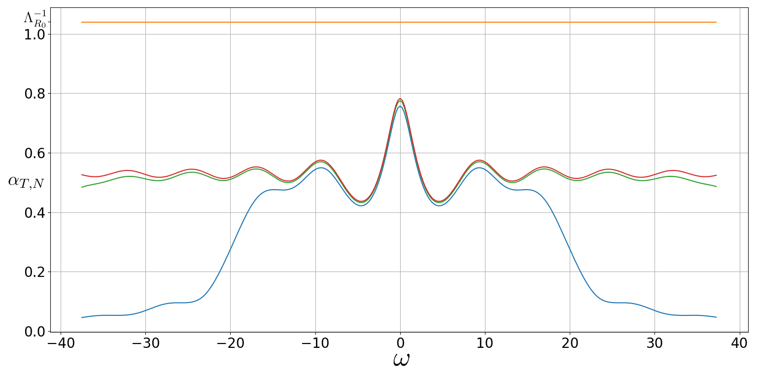
Figure 2. Graphs of the largest singular values $\alpha_{T,N}(-\nu_{0}+i\omega)$ versus $\omega$ computed via the numerical implementation of the approximation scheme Approximation scheme: statement-Approximation scheme: statement applied to (4.53) with $\alpha=0.6$, $\tau=0.83$ and $R=R_{0}(\alpha,\tau)$ given by Lemma 4.4. Parameters of the scheme are taken as $m=2$, $\Lambda=\Lambda_{R}$, $\nu_{0}=0.01$, $T=15$, $\Omega=37.5$ and $N=2$ (blue), $N=5$ (green), $N=10$ (red). Horizontal line (orange) passes through $\Lambda_{R_{0}}^{-1}$ on the vertical axis. See the repository for implementation details.

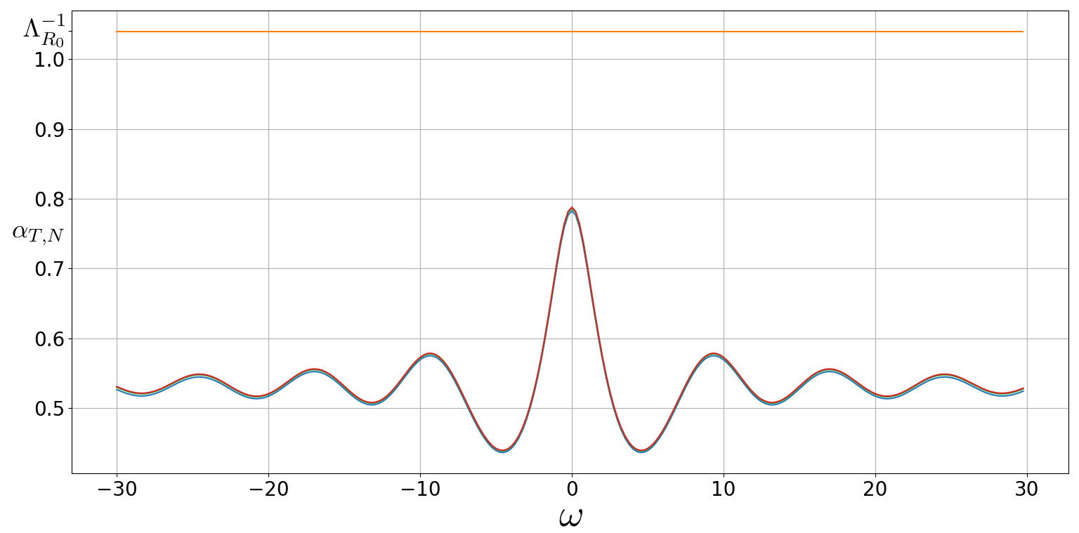
Figure 3. Graphs of the largest singular values $\alpha_{T,N}(-\nu_{0}+i\omega)$ versus $\omega$ computed via the numerical implementation of the approximation scheme Approximation scheme: statement-Approximation scheme: statement applied to (4.53) with $\alpha=0.6$, $\tau=0.83$ and $R=R_{0}(\alpha,\tau)$ given by Lemma 4.4. Parameters of the scheme are taken as $m=2$, $\Lambda=\Lambda_{R}$, $\nu_{0}=0.01$, $T=15$, $\Omega=30$ and $N=10$ (blue), $N=20$ (green), $N=30$ (red). Horizontal line (orange) passes through $\Lambda_{R_{0}}^{-1}$ on the vertical axis. See the repository for implementation details.

For $T=15$, Fig. 2 and Fig. 3 show graphs versus $\omega$ of the largest singular value $\alpha_{T,N}(-\nu_{0}+i\omega)$ of the matrix $W_{T,N}(-\nu_{0}+i\omega)$ from (4.43) for $N\in\{2,5,10\}$ and $N\in\{10,20,30\}$ respectively. For $T=25$, the conducted experiments give indistinguishable figures. This indicates convergence of the numerical scheme. For $|\omega|>10$ the curves tend to exhibit an oscillating pattern justifying Conjecture 1.

Analogous experiments justify the validity of the frequency inequality in the region $2\alpha\tau<1$ with $\alpha\in[0.5,1)$. Consequently, this region is expected to be contained in the region of global stability for (4.49). For $\alpha\in(0,0.5)$, the scheme indicates violation of the frequency inequality, but this is only a limitation of the method. We expect that one may improve the obtained results on the global stability by constructing more delicate invariant regions localizing the global attractor in the model.

4.6. Mackey-Glass equations

In this section, we study the following class of nonlinear scalar delay equations suggested by M.C. Mackey and L. Glass [20] as a model for certain physiological processes. It is described as

(4.56) $$\dot{x}(t)=-\gamma x(t)+\beta\frac{x(t-\tau)}{1+|x(t-\tau)|^{\kappa}},$$

where $\tau,\beta,\gamma>0$ and $\kappa>1$ are real parameters. From the physiological perspective, one is interested in the dynamics of (4.56) in the positive cone. However, for global analysis it is convenient to consider the system in the entire space.

Standard arguments show that (4.56) generates a dissipative semiflow $\varphi$ in the space $\mathbb{E}=C([-\tau,0];\mathbb{R})$ given by $\varphi^{t}(\phi_{0})=x_{t}$ for all $t\geq 0$ and $\phi_{0}\in\mathbb{E}$, where $x\colon[-\tau,\infty)\to\mathbb{R}$ is the classical solution to (4.56) with $x_{0}=\phi_{0}$. Recall that $x_{t}(\theta):=x(t+\theta)$ for $\theta\in[-\tau,0]$ denotes the $\tau$-history segment at $t\geq 0$. Consequently, there exists a global attractor $\mathcal{A}$.

In [2], it is shown that for $\beta\leq\gamma$, the global attractor $\mathcal{A}$ of $\varphi$ is given by the zero equilibrium $\phi^{0}(\cdot)\equiv 0$. For $\beta>\gamma$, the global attractor $\mathcal{A}$ lies in the ball of radius $\beta\gamma^{-1}\kappa^{-1}(\kappa-1)^{(\kappa-1)/\kappa}$ centered at $0$ and any ball with a radius not smaller than that is positively invariant w.r.t. $\varphi$.

It is not hard to see that for $\beta<\gamma$ there is a unique equilibrium $\phi^{0}(\cdot)\equiv 0$ with a negative leading real eigenvalue. For $\beta=\gamma$, the leading eigenvalue is $0$ and the system undergoes a pitchfork bifurcation at $\phi^{0}$ with a birth of the pair of symmetric equilibria $\phi^{+}$ and $\phi^{-}$ given by $\phi^{\pm}(\cdot)\equiv\pm(\beta\gamma^{-1}-1)^{1/\kappa}$ for $\beta>\gamma$.

Numerical experiments conducted in [20] indicate that the model (4.56) may posses chaotic behavior and, consequently, the attractor $\mathcal{A}$ may have rich structure. In particular, chaos is observed for $\gamma=0.1$, $\beta=0.2$, $\kappa=10$ and $\tau\geq 10$.

In [2], we estimated the Lyapunov dimension of $\mathcal{A}$ from above by the quantity $C(\gamma,\beta,\kappa)\cdot\tau+1$ with some $C(\gamma,\beta,\kappa)>0$. In particular, the estimate implies that the attractor $\mathcal{A}$ does not contain closed invariant contours provided that $\tau<C(\gamma,\beta,\kappa)^{-1}$. For $\beta=0.2$, $\gamma=0.1$ and $\kappa=10$ we have $C(\gamma,\beta,\kappa)\approx 0.9957$ and the inequality is close to $\tau\leq 1$. However, it can be verified that for $\tau=\tau_{0}$, where

(4.57) $$\tau_{0}=\frac{\arccos(-\frac{1}{4})}{0.4\cdot(1-\frac{1}{16})}\approx 4.8626,$$

the leading pair of complex-conjugate characteristic roots of $\phi^{\pm}$ crosses the imaginary axis and the system undergoes a supercritical Hopf bifurcation (in contrast to the Suarez-Schopf model, where the direction is subcritical). We expect the system to be globally stable for $\tau<\tau_{0}$ and conjecture that the same holds for any parameters as follows.

Conjecture 2.

For $\beta>\gamma>0$, $\tau>0$ and $\kappa>1$, the semiflow $\varphi$ generated by (4.56) is globally asymptotically stable provided that the equilibria $\phi^{\pm}=\pm(\beta\gamma^{-1}-1)^{1/\kappa}$ are linearly stable, i.e. all their characteristic roots have negative real parts.

In other words, the conjecture states that the boundary of global stability in (4.56) is determined from the local stability of the symmetric equilibria $\phi^{\pm}$, i.e. it is trivial in the terminology of N.V. Kuznetosv et al. [14]. This contrasts with the Suarez-Schopf oscillator (4.49), where the boundary is hidden. Now we are going to justify the conjecture by means of the developed machinery.

Firstly, it is convenient to normalize the delay in (4.56) by scaling the time variable $t\rightarrow\tau t$. Then (4.56) transforms into

(4.58) $$\dot{x}(t)=-\tau\gamma x(t)+\tau\beta\frac{x(t-1)}{1+|x(t-1)|^{\kappa}}.$$

Linearization of (4.58) along a given solution $y_{0}\colon[-1,\infty)\to\mathbb{R}$ gives

(4.59) $$\dot{x}(t)=-\tau\gamma x(t)+\tau\beta f^{\prime}(y_{0}(t-1))x(t-1),$$

where $f(y)=y/(1+|y|^{\kappa})$ for $y\in\mathbb{R}$ and $f^{\prime}(y)$ is the derivative of $f$ at $y$. Straightforward calculations show that $-\frac{(\kappa-1)^{2}}{4\kappa}\leq f^{\prime}(y)\leq 1\text{ for any }y\in\mathbb{R}$. From this, we rewrite (4.59) as (here $y_{0,t}$ is the $1$-history segment of $y_{0}(\cdot)$ at $t$)

(4.60) $$\dot{x}(t)=-\tau\gamma x(t)+(\tau\beta-\Lambda)x(t-1)+F^{\prime}(y_{0,t})x(t-1),$$

where $F^{\prime}(\phi)=\tau\beta(f^{\prime}(\phi(-1))-1)+\Lambda$ for $\phi\in C([-1,0];\mathbb{R})$ and $\Lambda$ is given by

(4.61) $$\Lambda=\frac{1}{2}\cdot\tau\beta\left(\frac{(\kappa-1)^{2}}{4\kappa}+1\right).$$

It is clear that $|F^{\prime}(\phi)|\leq\Lambda$.

We consider (4.60) in the context of (3.1) with $r_{1}=r_{2}=n=1$, $\widetilde{A}\phi=-\tau\gamma\phi(0)+(\tau\beta-\Lambda)\phi(-1)$ and $C\phi:=\phi(-1)$ for $\phi\in C([-1,0];\mathbb{R})$; $\widetilde{B}=1$; $F^{\prime}(\wp)$ defined above for $\wp\in\mathcal{P}:=C([-\tau,0];\mathbb{R})$ and $\pi:=\varphi$.

Eigenvalues of the operator $A$ corresponding via (3.4) to the operator $\widetilde{A}$ given above are constituted by the roots $p\in\mathbb{C}$ to

(4.62) $$-\tau\gamma+(\tau\beta-\Lambda)e^{-p}-p=0.$$

Let $\lambda_{1}(A)$, $\lambda_{2}(A)$, …be the eigenvalues arranged (according to their multiplicity) by nonincreasing of real parts. Then the spectral bound of $A^{[\wedge m]}$ is given by $\operatorname{Re}\lambda_{1}+\ldots+\operatorname{Re}\lambda_{m}$.

We have the following analog of Proposition 4.5 which gives a criterion for the absence of closed invariant contours on $\mathcal{A}$.

Proposition 4.6.

Let $\varphi$ be the semiflow generated by (4.56). Consider (4.60) in the context of (3.1) as it is stated below the former. Suppose there exists $\nu_{0}>0$ such that $\operatorname{Re}\lambda_{1}(A)+\operatorname{Re}\lambda_{2}(A)<-\nu_{0}$ and for $m=2$ the frequency inequality (3.53) with $\Lambda$ given by (4.61) is satisfied. Then the global attractor $\mathcal{A}$ of $\varphi$ does not contain closed invariant contours on which $\varphi^{t}$ is bijective for some $t>0$.

Proof.

Similarly to the proof of Theorem 4.5 we get that the Hausdorff dimension of $\mathcal{A}$ is strictly less than $2$.

Now let $\mathcal{B}_{R_{0}}(0)$ be the ball of radius $R_{0}$ centered at zero. As discussed above, for any $R_{0}\geq\beta\gamma^{-1}\kappa^{-1}(\kappa-1)^{(\kappa-1)/\kappa}$, the attractor $\mathcal{A}$ lies in $\mathcal{B}_{R_{0}}(0)$ and the ball is positively invariant. Then the conclusion follows from Corollary 2 in [18] by modulo that the statement therein requires $\varphi^{t}$ to be bijective on $\mathcal{A}$, but in the proof it is used only that $\varphi^{t}$ is bijective on the closed invariant contour as in Corollary 1 from the same work. The proof is finished. ∎

Remark 4.4.

Under the conditions of Proposition 4.6 we, in fact, have the robust condition

(4.63) $$\lambda_{1}(\Xi)+\lambda_{2}(\Xi)\leq-\nu_{0}<0,$$

for the first $\lambda_{1}(\Xi)$ and second $\lambda_{2}(\Xi)$ uniform Lyapunov exponents of the linearization cocycle $\Xi$ over $(C([-\tau,0];\mathbb{R}),\varphi)$ (see Remark 3.3). Thus, as in finite dimensions, it is expected that such a condition will guarantee the global stability.

Let us illustrate the method for $\gamma=0.1$, $\beta=0.2$, $\tau=4.5$ and $\kappa=10$. Here the leading pair of eigenvalues satisfies $\lambda_{1,2}(A)\approx-0.99\pm i1.12$. We consider the approximation scheme Approximation scheme: statement-Approximation scheme: statement for (4.60) with the given $\gamma$, $\beta$, $\tau$, $\kappa$ and $\Lambda$ given by (4.61). Parameters of the scheme are taken as $m=2$, $\Lambda$ as above, $\nu_{0}=0.01$, $\Omega\in\{30,37.5\}$, $T\in\{15,25\}$ and $N\in\{2,5,10,20,30\}$. We conduct numerical experiments using a realization of the scheme on Python (see Remark 4.3).

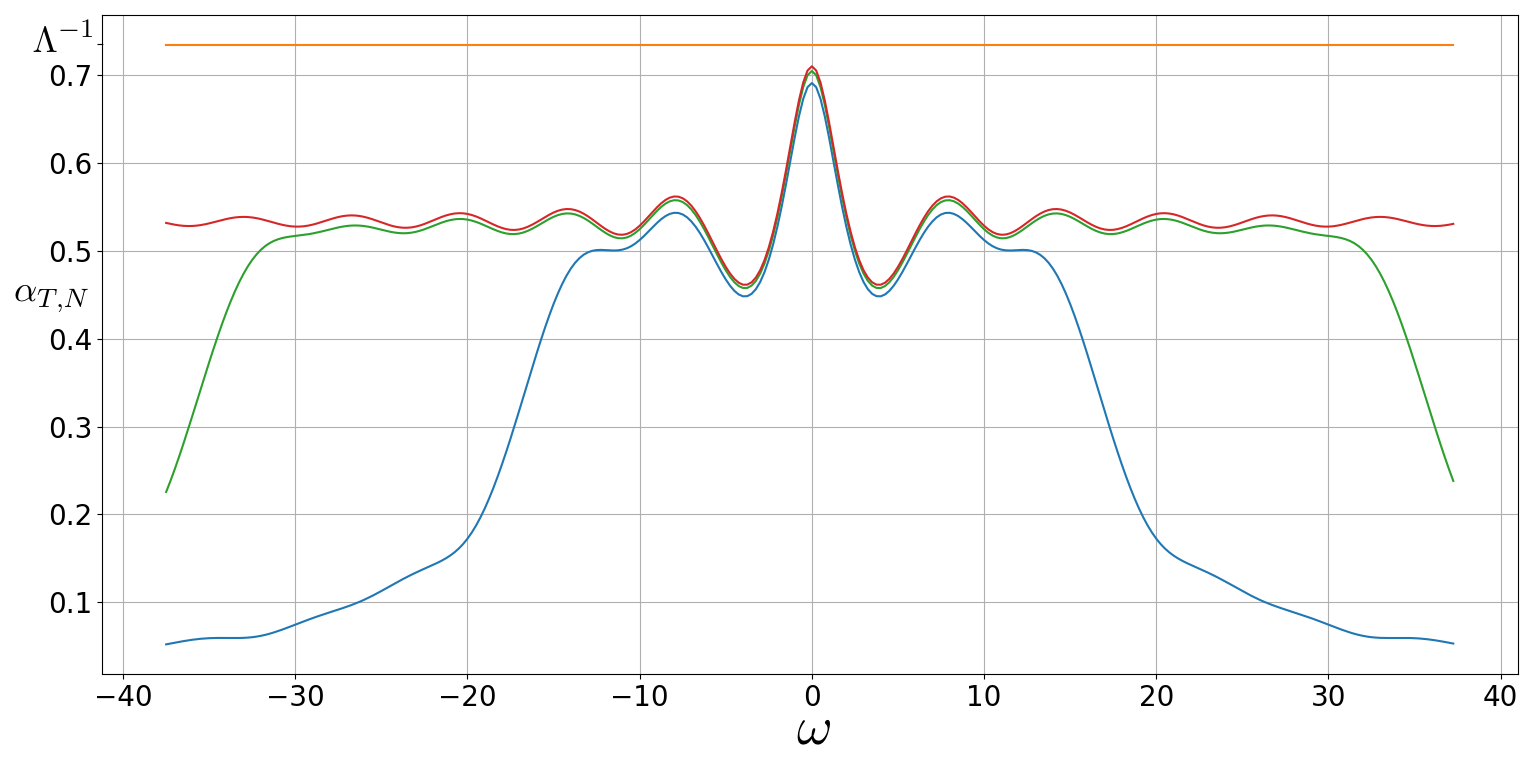
Figure 4. Graphs of the largest singular values $\alpha_{T,N}(-\nu_{0}+i\omega)$ versus $\omega$ computed via the numerical implementation of the approximation scheme Approximation scheme: statement-Approximation scheme: statement applied to (4.60) with $\gamma=0.1$, $\beta=0.2$, $\tau=4.5$ and $\Lambda$ given by (4.61). Parameters of the scheme are taken as $m=2$, $\Lambda$ as above, $\nu_{0}=0.01$, $T=15$, $\Omega=37.5$ and $N=2$ (blue), $N=5$ (green), $N=10$ (red). Horizontal line (orange) passes through $\Lambda^{-1}$ on the vertical axis. See the repository for implementation details.

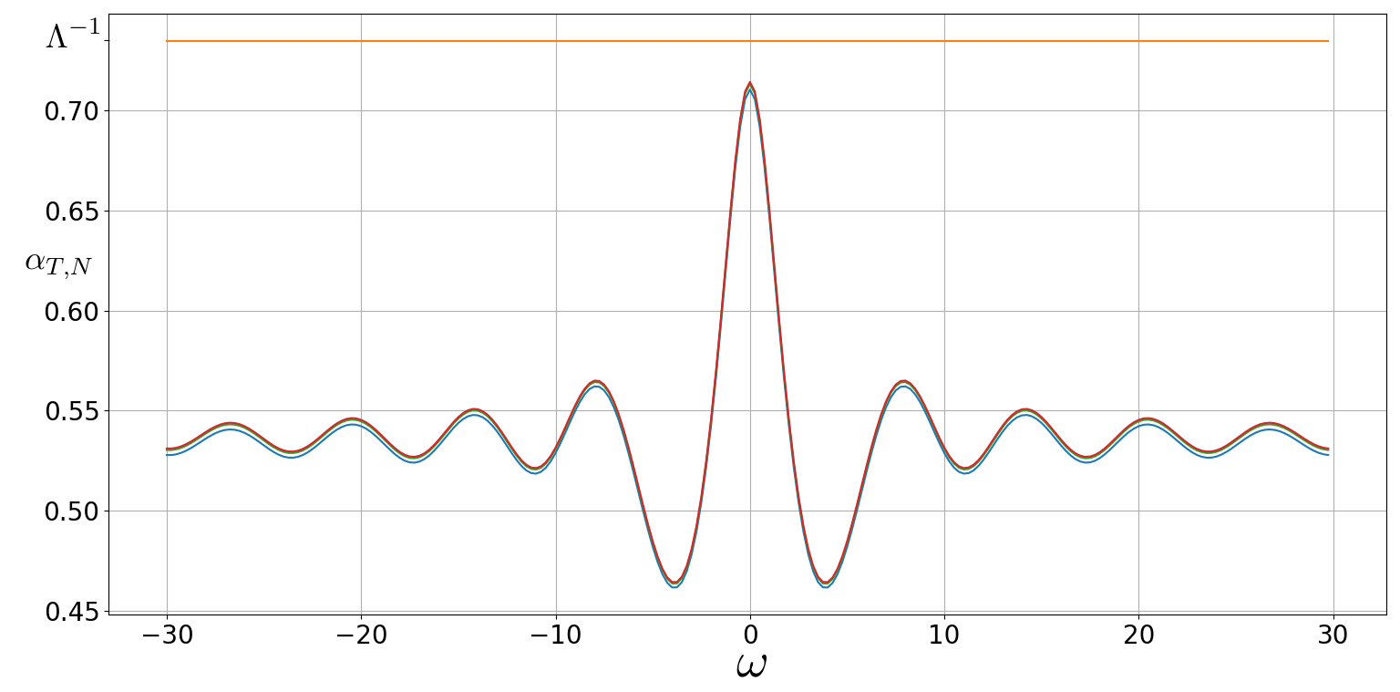
Figure 5. Graphs of the largest singular values $\alpha_{T,N}(-\nu_{0}+i\omega)$ versus $\omega$ computed via the numerical implementation of the approximation scheme Approximation scheme: statement-Approximation scheme: statement applied to (4.60) with $\gamma=0.1$, $\beta=0.2$, $\tau=4.5$ and $\Lambda$ given by (4.61). Parameters of the scheme are taken as $m=2$, $\Lambda$ as above, $\nu_{0}=0.01$, $T=15$, $\Omega=30$ and $N=10$ (blue), $N=20$ (green), $N=30$ (red). Horizontal line (orange) passes through $\Lambda^{-1}$ on the vertical axis. See the repository for implementation details.

For $T=15$, Fig. 4 and Fig. 5 show graphs of the largest singular value $\alpha_{T,N}(-\nu_{0}+i\omega)$ of $W_{T,N}(-\nu_{0}+i\omega)$ versus $\omega$ for $N\in\{2,5,10\}$ and $N\in\{10,20,30\}$ respectively. For $T=25$, the conducted experiments give indistinguishable figures. This indicates convergence of the numerical scheme. For $|\omega|>10$ the curves tend to exhibit an oscillating pattern justifying Conjecture 1.

In fact, the numerical scheme indicates that the frequency inequality is valid even for $\tau=4.6$, but the graphs come too close to the threshold line in the experiments. Analogous experiments justify the validity of the frequency inequality for $\tau\in(0,4.5]$. This indicates the absence of closed invariant contours in the system for such parameters and, as it is expected, the global stability (see Remark 4.4). Moreover, we find it very surprising, since the method is in a sense rough, that the achieved result turned out to be very close to the desirable one determined by the bifurcation parameter $\tau_{0}\approx 4.8626$ from (4.57). We consider this as another indicator that Conjecture 2 should be valid.

Data availability

The data that support the findings of this study can be generated using the scripts in the repository:

https://gitlab.com/romanov.andrey/freq-cond-compound-delay

Conflict of interest

The authors declare that they have no conflict of interest.

Funding

The reported study was funded by the Russian Science Foundation (Project 22-11-00172).

References

- [1] Anikushin M.M. Frequency theorem and inertial manifolds for neutral delay equations. J. Evol. Equ., 23, 66 (2023)
- [2] Anikushin M.M. Variational description of uniform Lyapunov exponents via adapted metrics on exterior products. arXiv preprint, arXiv:2304.05713v2 (2023)
- [3] Anikushin M.M. Spectral comparison of compound cocycles generated by delay equations in Hilbert spaces. arXiv preprint, arXiv:2302.02537v2 (2023)
- [4] Anikushin M.M., Romanov A.O. Hidden and unstable periodic orbits as a result of homoclinic bifurcations in the Suarez-Schopf delayed oscillator and the irregularity of ENSO. Phys. D: Nonlinear Phenom., 445, 133653 (2023)
- [5] Anikushin M.M. Nonlinear semigroups for delay equations in Hilbert spaces, inertial manifolds and dimension estimates, Differ. Uravn. Protsessy Upravl., 4, (2022)
- [6] Anikushin M.M. Inertial manifolds and foliations for asymptotically compact cocycles in Banach spaces. arXiv preprint, arXiv:2012.03821v2 (2022)
- [7] Anikushin M.M. Frequency theorem for parabolic equations and its relation to inertial manifolds theory, J. Math. Anal. Appl., 505(1), 125454 (2021)
- [8] Anikushin M.M. Almost automorphic dynamics in almost periodic cocycles with one-dimensional inertial manifold, Differ. Uravn. Protsessy Upravl., 2, (2021), in Russian
- [9] Ansmann G. Efficiently and easily integrating differential equations with JiTCODE, JiTCDDE, and JiTCSDE. Chaos, 28(4), 043116 (2018)
- [10] Chepyzhov V.V., Ilyin A.A. On the fractal dimension of invariant sets; applications to Navier-Stokes equations. Discrete Contin. Dyn. Syst., 10(1&2) 117–136 (2004)
- [11] Engel K.-J., Nagel R. One-Parameter Semigroups for Linear Evolution Equations. Springer-Verlag (2000)
- [12] Hale J.K. Theory of Functional Differential Equations. Springer-Verlag, New York (1977)
- [13] Kuznetsov N.V., Reitmann V. Attractor Dimension Estimates for Dynamical Systems: Theory and Computation. Switzerland: Springer International Publishing AG (2020)
- [14] Kuznetsov N.V., Mokaev T.N., Kuznetsova O.A., Kudryashova E.V. The Lorenz system: hidden boundary of practical stability and the Lyapunov dimension, Nonlinear Dyn., 102, 713–732 (2020)
- [15] Kuznetsov N.V. The Lyapunov dimension and its estimation via the Leonov method. Physics Letters A, 380(25–26) 2142–2149 (2016)
- [16] Leonov G.A., Boichenko V.A. Lyapunov’s direct method in the estimation of the Hausdorff dimension of attractors. Acta Appl. Math., 26(1), 1–60 (1992)
- [17] Li M.Y., Muldowney J.S. A geometric approach to global-stability problems. SIAM J. Math. Anal., 27(4), 1070–1083 (1996)
- [18] Li M.Y., Muldowney J.S. Lower bounds for the Hausdorff dimension of attractors. J. Dyn. Differ. Equ., 7(3), 457–469 (1995)
- [19] Li M.Y., Muldowney J.S. On R.A. Smith’s autonomous convergence theorem. Rocky Mt. J. Math., 365–379 (1995)
- [20] Mackey M.C., Glass L. Oscillation and chaos in physiological control systems. Science, 197(4300), 287–289 (1977)
- [21] Mallet-Paret J., Nussbaum R.D. Tensor products, positive linear operators, and delay-differential equations. J. Dyn. Diff. Equat., 25, 843–905 (2013)
- [22] Mallet-Paret J., Sell G.R. The Poincaré-Bendixson theorem for monotone cyclic feedback systems with delay. J. Differ. Equations, 125, 441–489 (1996)
- [23] Smith R.A. Some applications of Hausdorff dimension inequalities for ordinary differential equations. P. Roy. Soc. Edinb. A, 104(3-4), 235–259 (1986)
- [24] Suarez M.J., Schopf P.S. A delayed action oscillator for ENSO. J. Atmos. Sci., 45(21), 3283–3287 (1988)
- [25] Temam R. Infinite-Dimensional Dynamical Systems in Mechanics and Physics. Springer (1997)